An Improved Heap-Based Optimizer for Optimal Design of a Hybrid Microgrid Considering Reliability and Availability Constraints

Abstract

The hybrid microgrid system is considered one of the best solution methods for many problems, such as the electricity problem in regions without electricity, to minimize pollution and the depletion of fossil sources. This study aims to propose and implement a new algorithm called improved heap-based optimizer (IHBO). The objective of minimizing the microgrid system cost is to reduce the net present cost while respecting the reliability, power availability, and renewable fraction factors of the microgrid system. The results show that the PV/diesel/battery hybrid renewable energy system (HRES) gives the best solution, with a net present cost of MAD 120463, equivalent to the energy cost of MAD 0.1384/kWh. The reliability is about 3.89%, the renewable fraction is about 95%, and the power availability is near to 99%. The optimal size considered is represented as 167.3864 m² of PV area, which is equivalent to 44.2582 kW and 3.8860 kW of diesel capacity. The study results show that the proposed optimization algorithm of IHBO is better than the artificial electric field algorithm, the grey wolf optimizer, Harris hawks optimization, and the original HBO algorithm. A comparison of the net present cost with a different fuel price is carried out, in which it is observed that the net present cost is reduced even though its quantity used is mediocre.

1. Introduction

The implementation of hybrid microgrids is necessary due to their advantages. Many projects and studies have proven their essential ecological and economic effects. The literature has assessed the microgrid from all directions, including design, operation, optimization, control, and others. Literature reviews have provided more comprehensive studies. In [1], a comprehensive study on the optimization of microgrid operations has been presented. In [2], a review of AC and DC microgrid protection has been presented. Reference [3] presented a D.C. microgrid protection comprehensive review. Reference [4] presented a review on optimization and control techniques of the hybrid AC/DC microgrid, as well as the integration challenges. Reference [5] presented a comprehensive review of the planning, the operation, and the control of a DC microgrid. Reference [6] presented a review of microgrid sizing, design, and energy management.

The design and operation optimization of microgrids, considered the main objective of this work, has been presented in many papers. Reference [7] presented a design and assessment of the microgrid using a statistical methodology that calculates the effect of energy reliability and variability on microgrid performance. The paper used a REopt platform to explore the cost savings and revenue streams. In [8,9], the microgrid design has been investigated using several algorithms and configurations. In [10], a hybrid simulated annealing particle swarm (SAPS) algorithm has been presented to determine the microgrid optimal size that is subject to the economic and reliable operation constraints and to subsequently boost power supply security and stability. The paper [11] presented a new compromise method based on the Six Sigma approach to compare several multi-objective algorithms. The new approach has been applied to microgrid sizing and design based on PV, wind turbine, diesel, and battery systems. Reference [12] presented a graph-theoretic algorithm known as P-graph which allows the identification of optimal and near-optimal solutions for practical decision making. This study proposed a multi-period P-graph optimization framework for optimizing photovoltaic-based microgrids with battery-hydrogen energy storage. The proposed approach is demonstrated through two case studies. Reference [13] proposed a novel cash-flow model for Li-ion battery storage used in the energy system; the study considers the Li-ion battery degradation characteristic.

Optimization techniques are more competent in solving non-linear optimization problems, such as optimal reactive power dispatch (ORPD) [14], economic emission dispatch [15], intelligent energy management [16], and parameter estimation of photovoltaic models [17]. Reference [18] used an experimental validation of a lab-scale microgrid. Reference [19] concerns the undervoltage in smart distribution systems. The optimal power flow from attackers has been presented in [20].

The development of tools to design microgrids has become an important research area; the development of meta-heuristic algorithms begins a trend. In the literature, many papers presented different algorithms which have been applied to design a hybrid microgrid. In [21], an improved two-archive many-objective evolutionary algorithm (TA-MaEA) based on fuzzy decisions has been used to solve the sizing optimization problem for HRES. The simulation considered the following objective function: costs, probability of loss of power supply, pollutant emissions, and power balance. Reference [22] proposes an HRES of PV and fuel cells with an optimal total annual cost; the study used a new, improved metaheuristic called the amended water strider algorithm (AWSA). The reliability is considered, and the sensitivity analysis is applied. Reference [23] presents a microgrid design composed of PV, wind, an inverter, a rectifier, an electrolyzer, and a fuel cell. The paper used a modified seagull optimization technique to find the best cost of the optimal sizing. The proposed algorithm is compared with the original seagull optimization algorithm (SOA) and modified farmland fertility algorithm (MFFA). Reference [24] presents a new hybrid algorithm called IWO/BSA to resolve the microgrid design of any configuration, including PV/wind turbine (WT)/biomass/battery, PV/biomass, PV/diesel/battery, and WT/diesel/battery systems. The study’s objective is to obtain the best system with optimal cost, pollution, availability, and reliability. Reference [25] presents an adaptive version of the marine predators algorithm (AMPA) to design a PV/diesel/battery microgrid system. The objective function minimizes the annualized cost, respecting the ecologic and reliability factors of the system. The results are compared with PSO and HOMER. Reference [26] proposed an improved version of the bonobo optimizer (BO) based on the quasi-oppositional technique to resolve the design problem of the HRES considering the PV, wind turbines, battery, and diesel. A comparison between the traditional BO, the new QOBO, and other optimization techniques is investigated to prove the efficacy of QOBO. Reference [27] proposed a deterministic approach to size a PV, battery, anaerobic digestion, and biogas power plant to meet a demand load in Kenya. The levelized cost of energy (LCOE) is considered the objective function, while the energy imbalance between generation and demand is considered.

The present paper proposes a new tool consisting of platforms using an improved version of the HBO algorithm called IHBO. The improvement of the HBO algorithm depends on enhancing the performance of the HBO algorithm using the velocity equation from the particle swarm optimization (PSO) algorithm. This equation improves the convergence capability behavior and enables different diversified solutions in the search space, which is necessary for such an algorithm and achieves the fitness function’s optimal value. The proposed platforms design hybrid microgrid systems composed of PV, wind, diesel, and batteries. Two configurations are presented, and four algorithms are used in the comparison. In summary, the paper addresses the following points:

• An improved version of the conventional HBO algorithm is proposed with the aim of improving its performance;
• The conventional HBO and proposed IHBO algorithms are applied for optimal design of a hybrid microgrid system including RES (photovoltaic panels, wind turbines, and batteries) with diesel generators;
• In the designed microgrid, the reliability, availability and the renewable fraction constraints are considered;
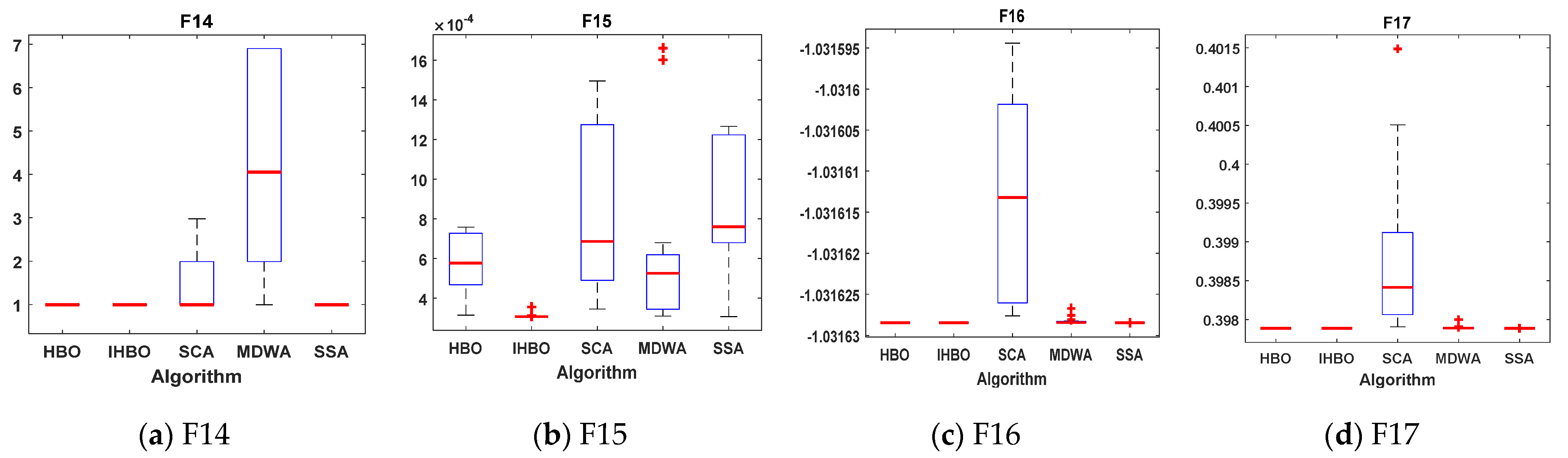
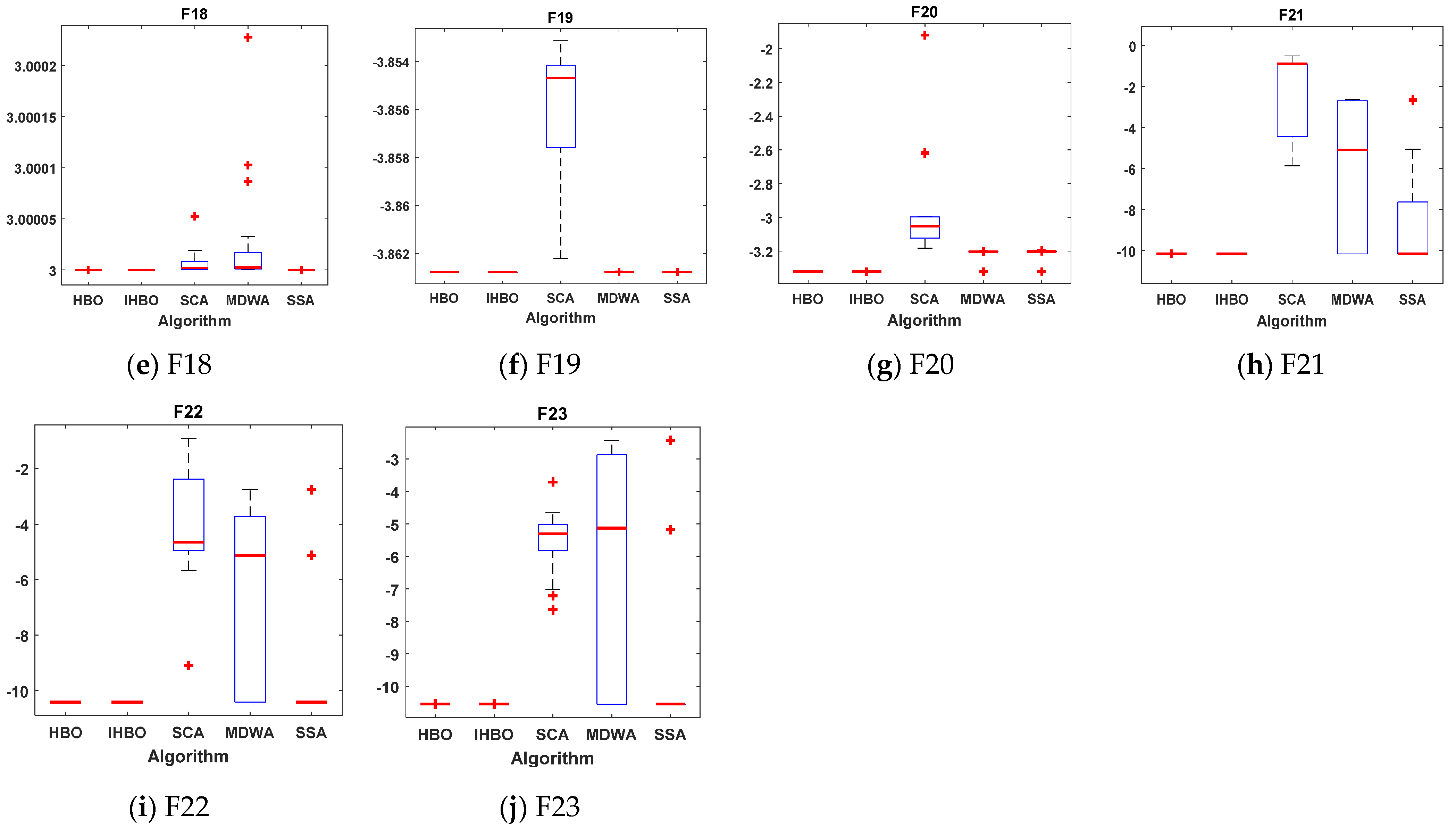
• The proposed IHBO algorithm’s efficiency and performance are evaluated on different benchmark functions, including the statistical measurement;
• The impact of the fuel price variation on the project investment is analyzed.

The paper is organized as follows: the introduction occurs in Section 1; the modeling of HRES components is contained in Section 2; Section 3 presents the objective functions and constraints; Section 4 presents the new, improved algorithm, namely IHBO; the results and discussion are presented in Section 5; and the conclusion is presented in Section 6.

2. HRES Components Modeling

2.1. PV Panel Modeling

The PV output power is calculated as follows [28,29]:

$$P_{pv}=I\langle t\rangle \times {\eta }_{pv}t\times A_{pv}$$

(1)

where $I$ represents the irradiation, ${\eta }_{pv}$ represents the efficiency of PV, and $A_{pv}$ is the area of PV. The efficiency of PV can be calculated based on reference efficiency (${\eta }_r$), the efficiency of MPPT (${\eta }_t$), temperature coefficient ($\beta$), ambient temperature ($T_a$), PV cell reference temperature ($T_r$) and nominal operating cell temperature (NOCT), as follows:

$${\eta }_{pv}\left(t\right)={\eta }_r\times {\eta }_t\times \left[1-\beta \times \left(T_a\langle t\rangle -T_r\right)-\beta \times I\langle t\rangle \times \left(\frac{NOCT-20}{800}\right)\times \left(1-{\eta }_r\times {\eta }_t\right)\right]$$

(2)

2.2. Wind System Modeling

The wind turbine output power can be calculated following these conditions [30]:

$$P_{wind}=\{\begin{array}{c}0, v\langle t\rangle \le v_{ci}, v\langle t\rangle \ge v_{co}\\ a\times {V\langle t\rangle }^3-b\times P_r, v_{ci}<v\langle t\rangle <v_r\\ P_r, v_r\le v\langle t\rangle <v_{co}\end{array}$$

(3)

where $V$ represents the wind velocity, $P_r$ is rated power, $v_{ci}$ is cut-in, $v_{co}$ represents cut-out, and $v_r$ is the rated wind. $a$ and$b$ are constant values that expressed as:

$$\begin{array}{c}a=P_r/\left(v_r{}^3-v_{ci}{}^3\right)\\ b=v_{ci}{}^3/\left(v_r{}^3-v_{ci}{}^3\right)\end{array}$$

(4)

The rated power of wind turbine can be calculated as:

$$P_r=\frac{1}{2}\times \rho \times A_{wind}\times C_p\times v_r{}^3$$

(5)

where $\rho$ is the air density, $A_{wind}$ represents the swept area of the wind turbine, and $C_p$ is the maximum power coefficient (from 0.25 to 0.45).

2.3. Diesel System Modeling

The diesel rated power can be calculated as [31]:

$$P_{dg}=\frac{F_{dg}\langle t\rangle -A_g\times P_{dg,out}}{B_g}$$

(6)

where $F_{dg}$ represents the fuel consumption, $P_{dg,out}$ is the output power of the diesel generator, and $A_g$ and $B_g$ are two constant values represent the fuel linear consumption.

2.4. Battery System Modeling

The battery capacity of the battery can be calculated as [31]:

$$C_{BESS}=\frac{E_l\times AD}{DOD\times {\eta }_i\times {\eta }_b}$$

(7)

where $E_l$ is the load demand, $AD$ is the autonomy of the battery which can lead power to the load on rainy days, $DOD$ represents the depth of discharge, and ${\eta }_i$ and ${\eta }_b$ represent the inverter and battery efficiency, respectively.

3. Objective Function and Constraints

3.1. Net Present Cost

The $\mathrm{NPC}$ represents an economic factor, which is considered the objective function in this study. The goal of the paper is to minimize the NPC, which is the sum of all costs during the project lifetime. The NPC is calculated as [32,33]:

$$\mathrm{NPC}=C+OM+R+F{C}_{dg}$$

(8)

where $C$ represent the capital cost, $OM$ is the operation and maintenance costs, $R$ is the replacement cost, and $F{C}_{dg}$ is the fuel cost.

3.2. LCOE Index

The LCOE represents the price of energy and is a critical factor which is calculated as [31]:

$$\mathrm{LCOE}=\frac{NPC\times CRF}{{{\displaystyle \sum }}_{t=1}^{8760}{P}_{load}t}$$

(9)

where CRF represents the capital recovery factor (obtained by converting the initial cost to annual capital cost), and $P_{load}$ represents the power load. The CRF is calculated as:

$$\mathrm{CRF}\left(ir,N\right)=\frac{i_r\times {\left(1+i_r\right)}^N}{{\left(1+i_r\right)}^R-1}$$

(10)

3.3. LPSP Index

The loss of power supply probability (LPSP) is a technical index that ranges from 0 to 1. It is used to indicate the reliability of the microgrid system. The LPSP is calculated as follows [31]:

$$\mathrm{LPSP}=\frac{{{\displaystyle \sum }}_{t=1}^{8760}\left(P_{load}\langle t\rangle -P_{pv}\langle t\rangle -P_{wind}\langle t\rangle +P_{dg,out}\langle t\rangle +E_{bmin}\right)}{{{\displaystyle \sum }}_{t=1}^{8760}{P}_{load}\langle t\rangle }$$

(11)

3.4. Renewable Energy Index

Renewable energy (RF) is calculated to determine the renewable energy percent that is penetrated into the microgrid system. The RF is expressed as [31]:

$$\mathrm{RF}=\left(1-\frac{{{\displaystyle \sum }}_{t=1}^{8760}{P}_{dg,out}\langle t\rangle }{{{\displaystyle \sum }}_{t=1}^{8760}{P}_{re}\langle t\rangle }\right)\times 100$$

(12)

where $P_{re}$ represents the sum of renewable energy powers.

3.5. Availability Index

The availability factor (Av) is assumed as an index of the customer’s satisfaction; it measures the ability of the microgrid to convert the total energy to load charge. The availability is calculated as [33]:

$$\mathrm{Av}=1-\frac{DMN}{{{\displaystyle \sum }}_{t=1}^{8760}{P}_{load}\langle t\rangle }$$

(13)

$$DMN=P_{bmin}\langle t\rangle -P_b\langle t\rangle -\left(P_{pv}\langle t\rangle +P_{wind}\langle t\rangle +P_{dg,out}\langle t\rangle -P_{load}\langle t\rangle \right)\times u\langle t\rangle$$

(14)

where $P_{bmin}$ represents the battery min state, $P_b$ represents the battery power, and $u$ is a fixed value which equals $1$ when the load is not satisfied and which equals $0$ otherwise.

3.6. Constraints

Constraints are introduced to tune the microgrid system factors and help to improve the microgrid service quality. In this work, the constraints proposed are:

$$\{\begin{array}{c}0\le A_{pv}\le A_{pv}^{max}\\ 0\le A_{wind}\le A_{wind}^{max}\\ 0\le P_{dg}\le P_{dg}^{max}\\ 0\le C_{BESS}\le C_{BESS}^{max}\\ LPSP\le {\mathrm{LPSP}}^{max}\\ {\mathrm{RF}}^{min}\le RF\\ A{v}^{min}\le Av\\ {\mathrm{AD}}^{min}\le AD\end{array}$$

(15)

where ${\mathrm{LPSP}}^{max}$ = 0.05, ${\mathrm{RF}}^{min }$ = 70%, ${\mathrm{Av}}^{min}$ = 90%, and ${\mathrm{AD}}^{min}$ = 1 day. The sizing limit is different from configuration to the others. All other parameters are shown in

Table A1. Summary of the HRES parameters.

Symbol	Quantity	Conversion
N	Project lifetime	20 year
${\eta }_r$	Reference efficiency of the PV	25%
${\eta }_t$	Efficiency of MPPT	100%
$T_r$	PV cell reference temperature	25 °C
$\beta$	Temperature coefficient	0.005 °C
NOCT	Nominal operating cell temperature	47 °C
$N_{pv}$	PV system lifetime	20 year
$C_p$	Maximum power coefficient	48%
$V_{ci}$	Cut-in wind speed	2.6 m/s
$V_{co}$	Cut-out wind speed	25 m/s
$V_r$	Rated wind speed	9.5 m/s
$N_{wind}$	Wind system lifetime	20 year
$p_f$	Fuel price in Morocco	MAD 0.96/L
$N_{diesel}$	Diesel system lifetime	7 year
$DOD$	Depth of discharge	80%
${\eta }_b$	Battery efficiency	97%
$N_{bat}$	Battery system lifetime	5 year
${\eta }_{inv}$	Inverter efficiency	97%

.

4. Proposed Algorithm

4.1. Heap-Based Optimizer (HBO)

The heap-based optimizer algorithm (HBO) is inspired by the social behavior of human beings [34]. One sort of social interaction between human beings can be observed in organizations where people in teams are arranged in a hierarchy for achieving a specific target; this is known as corporate rank hierarchy (CRH). CRH is presented in Figure 1a. The HBO algorithm is based on CRH in a very distinctive manner. In this regard, the concept of CRH is to arrange the search agents based on their suitability in this hierarchy using a heap tree-based data structure to enact the implementation of priority queues. Figure 1b shows an example of 3 degrees (3-ary) of min-heap. Three types of employees’ behaviors were used in the HBO algorithm. These types are: (i) the interaction of subordinates with their immediate head; (ii) the interaction between co-workers; and (iii) the self-contribution of individuals.

The mapping of the heap concept is divided into four steps:

A. 

Modeling the corporate rank hierarchy

Figure 2 displays the procedure of CRH modeling through a heap data structure, wherein xi is the ith search agent of the population. The curve in the objective space describes the shape of the supposed objective function, and the search agents are drawn on the fitness shape according to their convenience.

B. 

Mathematically modeling the collaboration with the boss

In a centralized organizational structure, the regulations and policies are enforced from the upper levels, and subordinates must follow their direct manager.

This can be mathematically described by updating the agent position of each search as follows:

$$x_i^k\left(t+1\right)=B^k+\gamma {\lambda }^k\left|B^k-x_i^k\left(t\right)\right|$$

(16)

$$\gamma =\left|2-\frac{\left(t mod \frac{T}{C}\right)}{\frac{T}{4C}}\right|$$

(17)

$${\lambda }^k=\left(2r-1\right)$$

(18)

where t is the current iteration, k is the kth component of a vector, B denotes the parent node, r is a random number from the range [0, 1], T is the maximum number of iterations, and C represents a user-defined parameter.

C. 

Mathematically modeling the interaction between the colleagues

Colleagues cooperate and perform official tasks. It is assumed in a heap that the nodes at the same level are colleagues, and each search agent x_i updates its location based on its randomly selected colleague S_r as follows:

$$x_i^k\left(t+1\right)=\{\begin{array}{c}{s}_r^k+\gamma {\lambda }^k\left|s_r^k-x_i^k\left(t\right)\right|, f\left(S_r\right)<f\left(x_i\left(t\right)\right)\\ x_i^k+\gamma {\lambda }^k\left|s_r^k-x_i^k\left(t\right)\right|, f\left(S_r\right)\ge f\left(x_i\left(t\right)\right)\end{array}$$

(19)

D. 

Self-contribution of an employee to accomplish a task

In this phase, the self-contribution of a worker is mapped as follows:

$$x_i^k\left(t+1\right)=x_i^k\left(t\right)$$

(20)

The following part explains how exploration can be controlled with this equation.

E. 

putting all together

The principal challenge is determining the selection probabilities for the three equations to balance exploration and exploitation. The purpose of the roulette wheel is to achieve a balance of possibilities. The roulette wheel is divided into three parts: p₁, p₂, and p₃. The value of p₁ makes a population changes their position, and it is calculated from the following equation:

$$p_1=1-\frac{t}{T}$$

(21)

The selection of p₂ is computed from the following equation:

$$p_2=p_1-\frac{1-p_1}{2}$$

(22)

Finally, the selection of p₃ is calculated as follows:

$$p_3=p_2-\frac{1-p_1}{2}=1$$

(23)

Accordingly, a general position-updating mechanism of the HBO algorithm is mathematically represented as follows:

$$x_i^k(t+1)=\{\begin{array}{c}{x}_i^k(t),p\le p_1\\ B^k+\gamma {\lambda }^k|B^k-x_i^k(t)|,p>p_1 and p\le p_2\\ s_r^k+\gamma {\lambda }^k|s_r^k-x_i^k(t)|,p>p_2 and p\le p_3 and f(S_r)<f(x_i(t))\\ x_i^k+\gamma {\lambda }^k|s_r^k-x_i^k(t)|,p>p_2 and p\le p_3 and f(S_r)\ge f(x_i(t))\end{array}$$

(24)

where p is a random number in the range (0, 1).

4.2. Improved Heap-Based Optimizer(IHBO)

In order to enhance the strength of the proposed IHBO algorithm for many high-dimensional optimization problems, core aspects of one of the most used meta-heuristic algorithms, PSO, are utilized. The PSO algorithm is introduced by [35]. The velocity equation from the PSO algorithm is used in the proposed IHBO algorithm. This modification leads to the improvement of the ability of the global search and enhances the local search capabilities of the improved algorithm. This core equation is as follows:

$$V_i^k\left(t+1\right)=w·V_i^k\left(t\right)+C_1·r_1\times (p_{best}-x_i^k\left(t\right))+C_2·r_2\times (g_{best}-x_i^k\left(t\right))$$

(25)

$$x_i^k\left(t+1\right)=x_i^k\left(t\right)+V_i^k\left(t+1\right)$$

(26)

where $C_1=C_2=0.5$, as these values gave the best solution in [36]; $w=0.7$; $r_1$ and $r_2$ are a random number in the range (0, 1)$; p_{best}$ is the best solution of an individual population, and $g_{best}$ is the best solution so far.

The flow chart of the proposed IHBO algorithm is shown in Figure 3.

Performance of the Proposed IHBO Algorithm

The proposed IHBO algorithm’s efficiency and performance are evaluated on different benchmark functions, including statistical measurements, such as minimum values, mean values, maximum values, and standard deviation (STD) for best solutions obtained by the proposed IHBO algorithm and the other recent optimization algorithms. The results obtained with the proposed IHBO technique is compared with three well-known optimization algorithms, including the sine cosine algorithm (SCA) [37], salp swarm algorithm (SSA) [38], movable damped wave algorithm (MDWA) [39], and the original heap-based optimizer (HBO).

Table 1. Parameter settings of the selected techniques.

Algorithms	Parameter Settings
Common settings	Population size: nPop = 50 Maximum iterations: Max_iter = 1000 Number of independent runs: 20
SSA	c2 = rand; c3 = rand
MDWA	amax = 1; amin = 0
SCA	A = 2
IHBO	sv = 100; degree = 3; w = 0.7; C1 = 0.5; C2 = 0.5; r1 = rand; r2 = rand
HBO	sv = 100; degree = 3

shows the parameters of all compared algorithms (SSA, MDWA, SCA, IHBO, and HBO). Qualitative metrics on F1, F4, F7, F9, F11, F12, F15, and F18, including 2D views of the functions, search history, average fitness history, and convergence curve, are presented in Figure 4.

Table 2. Results of unimodal benchmark functions.

Function		HBO	IHBO	SCA	MDWA	SSA
F1	Best	8.81 × 10−65	3.11× 10−86	5.61 × 10−41	1.34 × 10−44	2.21 × 10−10
	Worst	7.28 × 10−59	3.81× 10−81	1.24 × 10−28	3 × 10−39	8.48 × 10−10
	Mean	4 × 10−60	3.72× 10−82	8.72 × 10−30	3.01 × 10−40	5.63 × 10−10
	std	1.63 × 10−59	8.56× 10−82	2.92 × 10−29	8.19 × 10−40	1.99 × 10−10
F2	Best	1.24 × 10−39	4.59× 10−53	6.81 × 10−27	1.14 × 10−22	2.69 × 10−06
	Worst	4.86 × 10−37	1.2× 10−49	1.84 × 10−19	2.86 × 10−22	1.54 × 10−05
	Mean	5.65 × 10−38	1.99× 10−50	9.67 × 10−21	1.89 × 10−22	6.7 × 10−06
	std	1.12 × 10−37	3.32× 10−50	4.11 × 10−20	4.64 × 10−23	2.62 × 10−06
F3	Best	2.24 × 10−09	3 × 10−16	1.42 × 10−19	5.59× 10−22	3.12 × 10−10
	Worst	2.29 × 10−05	1.8 × 10−11	4.44 × 10−12	5.44× 10−13	1.84 × 10−09
	Mean	1.78 × 10−06	1.45 × 10−12	2.57 × 10−13	3.52× 10−14	1.14 × 10−09
	std	5.22 × 10−06	4.09 × 10−12	9.86 × 10−13	1.21× 10−13	4.43 × 10−10
F4	Best	8.73 × 10−14	2.76× 10−16	1.04 × 10−13	1.67 × 10−15	7.74 × 10−06
	Worst	1.94 × 10−10	1.5× 10−13	3.01 × 10−08	1.72 × 10−11	1.73 × 10−05
	Mean	2.54 × 10−11	2.05× 10−14	2 × 10−09	2.27 × 10−12	1.25 × 10−05
	std	4.6 × 10−11	3.92× 10−14	6.71 × 10−09	4.03 × 10−12	2.36 × 10−06
F5	Best	0.072812	0.010245	6.364761	0.068609	4.046853
	Worst	8.553338	4.229361	8.078748	4.466474	600.9202
	Mean	1.999632	1.430528	6.967484	0.879403	73.87534
	std	2.507143	1.504423	0.50586	1.21085	150.4287
F6	Best	0.00	0.00	7.99 × 10−02	6.83 × 10−06	2.94 × 10−10
	Worst	1.23 × 10−32	0.00	5.71 × 10−01	1.11 × 10−04	8.89 × 10−10
	Mean	1.23 × 10−33	0.00	3.12 × 10−01	2.93 × 10−05	5.74 × 10−10
	std	3.79 × 10−33	0.00	1.35 × 10−01	2.67 × 10−05	1.60 × 10−10
F7	Best	7.43 × 10−04	3.54 × 10−04	5.78× 10−05	2.88 × 10−04	6.27 × 10−04
	Worst	3.22 × 10−03	3.30 × 10−03	1.82× 10−03	4.33 × 10−03	1.49 × 10−02
	Mean	1.99 × 10−03	1.50 × 10−03	6.88× 10−04	1.46 × 10−03	4.60 × 10−03
	std	7.46 × 10−04	7.90 × 10−04	5.20× 10−04	1.23 × 10−03	3.22 × 10−03
The best values obtained are in bold.

,

Table 3. Results of multimodal benchmark functions.

Function		HBO	IHBO	SCA	MDWA	SSA
F8	Best	−4189.83	−4189.83	−2724.77	−2752.03	−3262.03
	Worst	−4189.83	−4189.83	−1976.68	−1566.57	−2423.89
	Mean	−4189.83	−4189.83	−2297.91	−2116.51	−2851.97
	std	1.87× 10−12	1.87× 10−12	187.9469	338.86	263.4202
F9	Best	0.00	0.00	0.00	0.00	4.974795
	Worst	0.00	0.994959	19.68757	0.00	24.87393
	Mean	0.00	0.049748	0.984379	0.00	13.82991
	std	0.00	0.22248	4.402275	0.00	5.448648
F10	Best	4.44 × 10−15	4.44 × 10−15	4.44 × 10−15	8.88× 10−16	6.91 × 10−06
	Worst	4.44× 10−15	4.44× 10−15	2.43 × 10−12	7.99 × 10−15	2.01 × 10+00
	Mean	4.44× 10−15	4.44× 10−15	1.26 × 10−13	4.44 × 10−15	1.58 × 10−01
	std	0.00	0.00	5.43 × 10−13	1.15 × 10−15	5.07 × 10−01
F11	Best	0.00	0.00	0.00	0.00	7.38 × 10−02
	Worst	1.06 × 10−09	2.46 × 10−02	1.31 × 10−01	0.00	6.13 × 10−01
	Mean	5.32 × 10−11	2.59 × 10−03	8.38 × 10−03	0.00	2.77 × 10−01
	std	2.38 × 10−10	6.16 × 10−03	2.96 × 10−02	0.00	1.51 × 10−01
F12	Best	4.71× 10−32	4.71× 10−32	1.85 × 10−02	9.67 × 10−07	3.46 × 10−12
	Worst	4.81× 10−32	4.71× 10−32	9.96 × 10−02	1.31 × 10−04	3.12 × 10+00
	Mean	4.72× 10−32	4.71× 10−32	6.12 × 10−02	2.06 × 10−05	3.30 × 10−01
	std	2.16 × 10−34	5.62× 10−48	2.05 × 10−02	3.56 × 10−05	7.87 × 10−01
F13	Best	1.35× 10−32	1.35× 10−32	5.71 × 10−02	2.48 × 10−06	1.51 × 10−11
	Worst	1.84 × 10−32	1.35× 10−32	3.59 × 10−01	3.70 × 10−04	1.10 × 10−02
	Mean	1.37 × 10−32	1.35× 10−32	2.16 × 10−01	4.53 × 10−05	1.65 × 10−03
	std	1.10 × 10−33	2.81× 10−48	7.48 × 10−02	8.66 × 10−05	4.03 × 10−03
The best values obtained are in bold.

and

Table 4. Results of composite benchmark functions.

Function		HBO	IHBO	SCA	MDWA	SSA
F14	Best	9.98× 10−01	9.98× 10−01	9.98× 10−01	9.98× 10−01	9.98× 10−01
	Worst	9.98× 10−01	9.98× 10−01	2.98 × 10+00	6.90 × 10+00	9.98× 10−01
	Mean	9.98× 10−01	9.98× 10−01	1.49 × 10+00	4.12 × 10+00	9.98× 10−01
	std	0.00	0.00	8.81 × 10−01	2.51 × 10+00	1.25 × 10−16
F15	Best	3.15 × 10−04	3.07× 10−04	3.46 × 10−04	3.10 × 10−04	3.07× 10−04
	Worst	7.59 × 10−04	3.56× 10−04	1.50 × 10−03	1.66 × 10−03	1.27 × 10−03
	Mean	5.77 × 10−04	3.10× 10−04	8.01 × 10−04	5.92 × 10−04	9.01 × 10−04
	std	1.55 × 10−04	1.08× 10−05	3.78 × 10−04	3.77 × 10−04	3.21 × 10−04
F16	Best	−1.03163	−1.03163	−1.03163	−1.03163	−1.03163
	Worst	−1.03163	−1.03163	−1.03159	−1.03163	−1.03163
	Mean	−1.03163	−1.03163	−1.03161	−1.03163	−1.03163
	std	2.28× 10−16	2.28× 10−16	1.2 × 10−05	4.18 × 10−07	4.92 × 10−15
F17	Best	0.397887	0.397887	0.397907	0.397887	0.397887
	Worst	0.397887	0.397887	0.401488	0.397999	0.397887
	Mean	0.397887	0.397887	0.398743	0.397896	0.397887
	std	0.00	0.00	0.000945	2.48 × 10−05	1.1 × 10−14
F18	Best	3	3	3	3	3
	Worst	3	3	3.000052	3.000228	3
	Mean	3	3	3.000007	3.000026	3
	std	6.03× 10−16	1.11 × 10−15	1.2 × 10−05	5.53 × 10−05	5.2 × 10−14
F19	Best	−3.86278	−3.86278	−3.86221	−3.86278	−3.86278
	Worst	−3.86278	−3.86278	−3.85312	−3.86276	−3.86278
	Mean	−3.86278	−3.86278	−3.85612	−3.86278	−3.86278
	std	2.28× 10−15	2.28× 10−15	0.003147	5.9 × 10−06	1.22 × 10−14
F20	Best	−3.322	−3.322	−3.18286	−3.32199	−3.322
	Worst	−3.322	−3.322	−1.92056	−3.20299	−3.1952
	Mean	−3.322	−3.322	−2.9198	−3.21496	−3.22015
	std	4.56× 10−16	5.19 × 10−16	0.37441	0.036596	0.043929
F21	Best	−10.1532	−10.1532	−5.86842	−10.1532	−10.1532
	Worst	−10.1532	−10.1532	−0.49729	−2.63044	−2.63047
	Mean	−10.1532	−10.1532	−2.22823	−6.14446	−8.6434
	std	3.43× 10−15	3.65 × 10−15	1.885656	3.476701	2.751568
F22	Best	−10.4029	−10.4029	−9.10162	−10.4029	−10.4029
	Worst	−10.4029	−10.4029	−0.90756	−2.75188	−2.7659
	Mean	−10.4029	−10.4029	−4.00724	−6.90966	−9.37553
	std	3.21 × 10−15	2.51× 10−15	2.111063	3.308424	2.548
F23	Best	−10.5364	−10.5364	−7.64188	−10.5363	−10.5364
	Worst	−10.5364	−10.5364	−3.70826	−2.42157	−2.42734
	Mean	−10.5364	−10.5364	−5.51857	−6.16316	−9.86292
	std	1.78× 10−15	1.95 × 10−15	0.95525	3.420207	2.120365
The best values obtained are in bold.

tabulate the statistical results of the proposed IHBO algorithm and other well-known algorithms when applied for unimodal benchmark functions, named F1 to F7, multimodal benchmark functions, named F8 to F13, and composite benchmark functions, named F14 to F23, respectively. The best values, shown in bold, were achieved with the proposed IHBO algorithm, as well as MDWA and SCA, but the proposed IHBO technique achieves the best results for most of the benchmark functions. The convergence curves of all algorithms for the unimodal benchmark functions are shown in Figure 5 while Figure 6 shows the boxplots of each algorithm for these unimodal benchmark functions. Figure 7 displays the convergence characteristics curves of all algorithms for the multi-modal benchmark functions. The boxplots for each algorithm for these types of benchmark functions are presented in Figure 8. The convergence curves of all algorithms for the composite benchmark functions are displayed in Figure 9 while Figure 10 illustrates the boxplots for each algorithm for these benchmark functions. The proposed algorithm reached a stable point for all functions. Also, the boxplots of the proposed IHBO technique are very narrow for most functions compared to the other algorithms.

5. Project Implementation Location

The project was implemented in a small region in the west of Morocco called Terfaya, at coordinating latitude 27.932 and longitude −12.935.

6. Results and Discussion

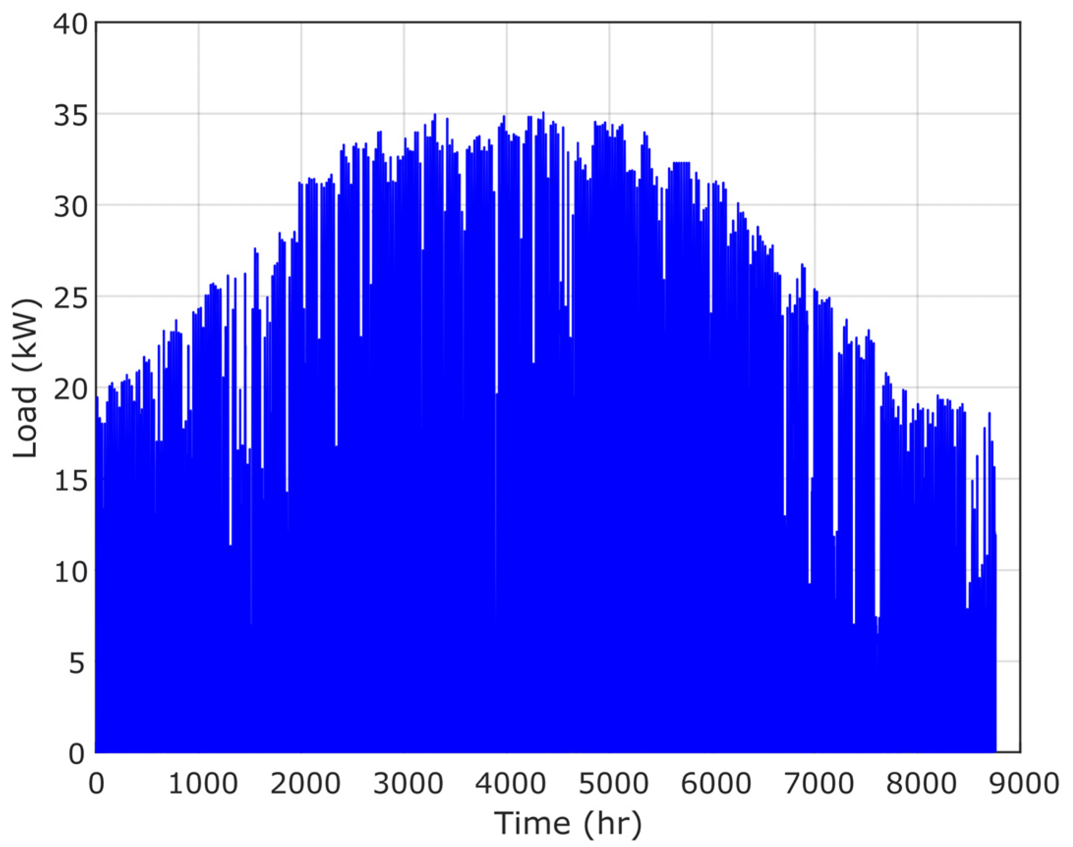
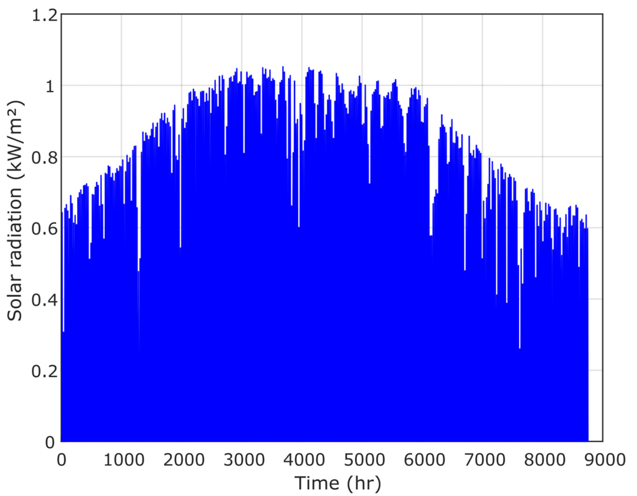
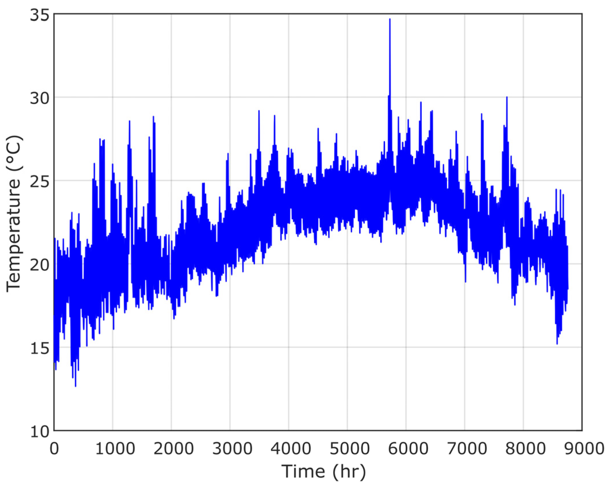
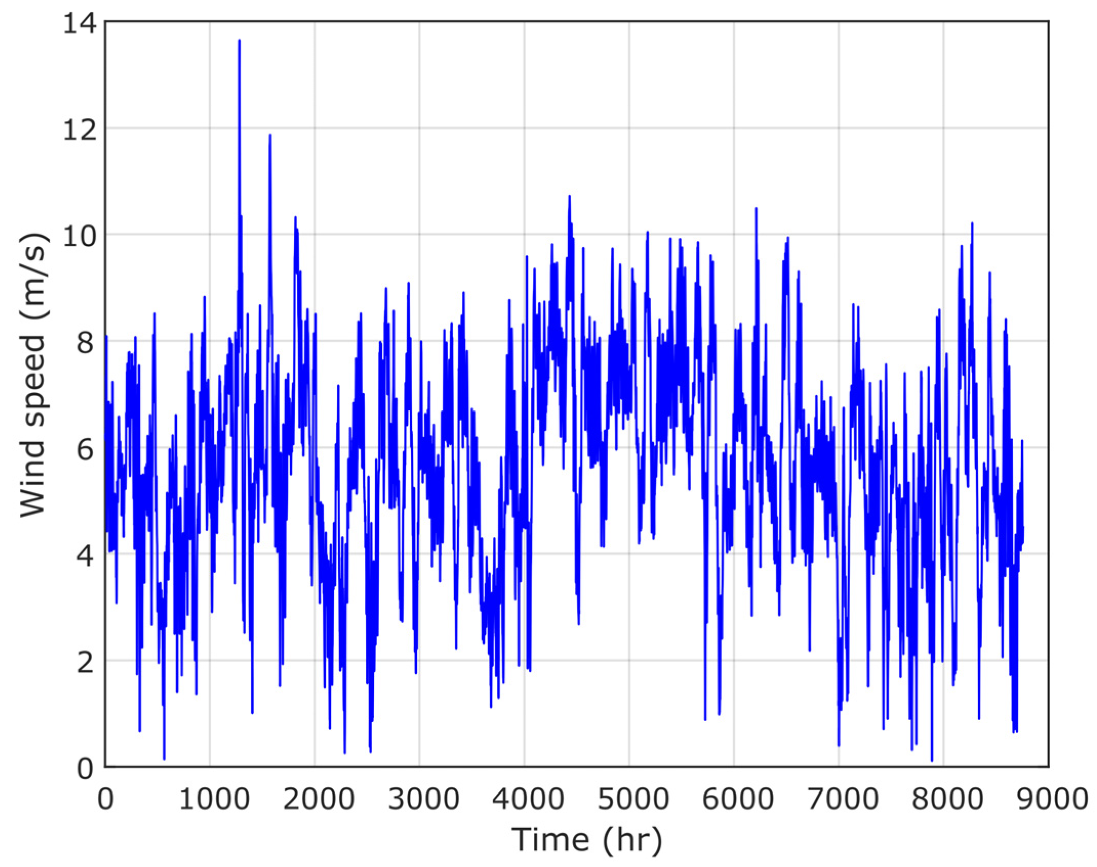
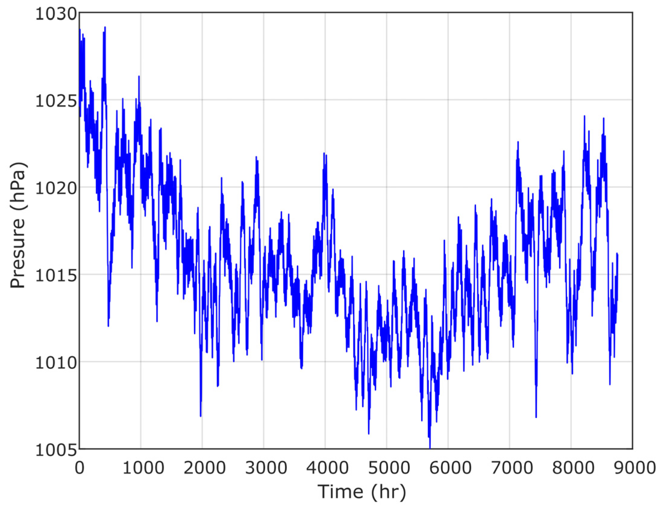
In this paper, the Terfaya region of Morocco is selected as the case study to implement an HRES platform based on an improved optimization algorithm called IHBO. The maps for the project location, the load charge, the annual ambient radiation, temperature, wind speed, and pressure are presented in Figure 11, Figure 12, Figure 13, Figure 14 and Figure 15, respectively.

The proposed HRES includes two renewable sources (PV and wind turbines), a diesel generator, and a battery storage system. According to the mathematical modeling of the mentioned systems, the PV output can be affected by the solar radiation data; otherwise, the output power of the wind is influenced by the wind speed data. The decision variables in this study are dedicated to the size of the HRES where: x(1) is the PV area ($A_{pv}$,), x(2) is the wind swept area ($A_{wind}$), x(3) represents the battery capacity ($C_{BESS}$) and x(4) is the rated power of the diesel generator ($P_{dg}$). In this paper, an analysis of fuel price variation is carried out.

6.1. Optimal HRES Design of PV/Diesel/Battery and PV/Wind/Diesel/Battery

6.1.1. PV/Diesel/Battery HRES

The results of the optimal HRES design for the case study concerning the PV/diesel/battery HRES are summarized in

Table 5. Results of the PV/diesel/battery HRES.

Algorithm	NPC (MAD)	LCOE (MAD/kWh)	LPSP	RF (%)	Availability (%)
AEFA	169,142	0.1361	0.0360	99.7905	98.5686
GWO	191,661	0.1543	0.0386	99.6961	98.6947
HHO	147,527	0.1187	0.0269	99.7289	98.5725
HBO	175,321	0.1411	0.0383	95.5051	98.9342
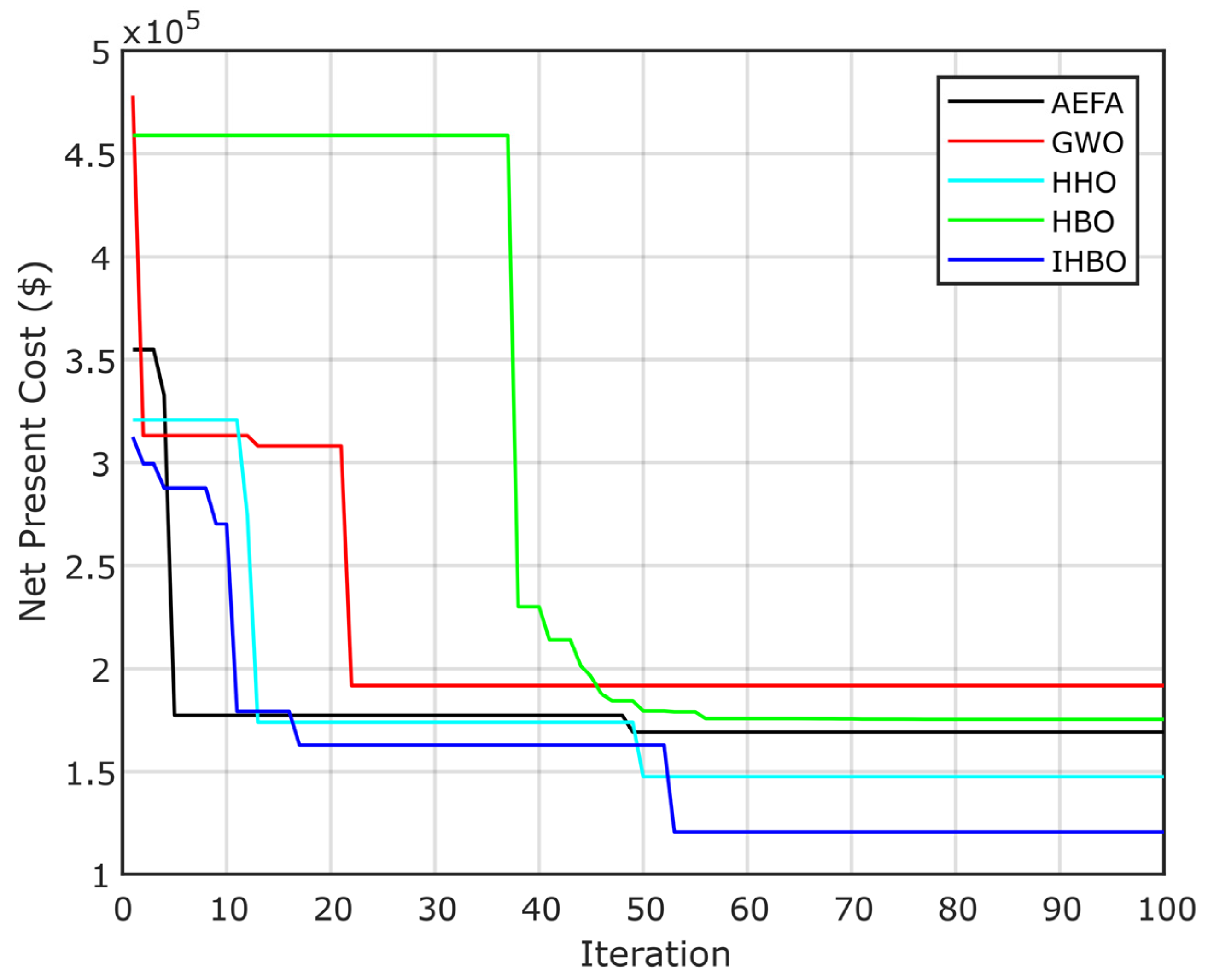
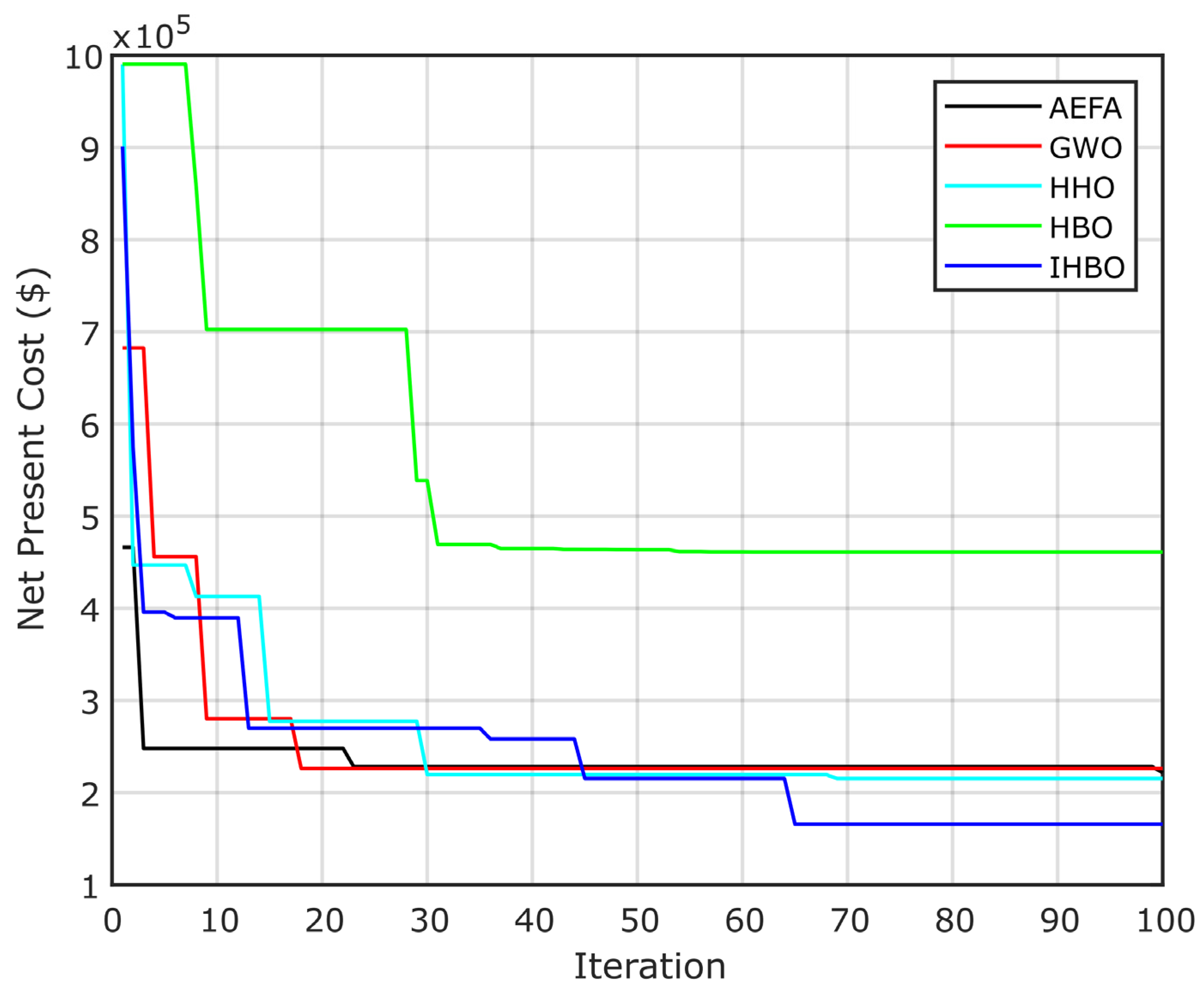
IHBO	120,463	0.1384	0.0389	95.3802	98.8665

. The table presents all used algorithms concerning the predefined constraints, including the LPSP, RF, and the availability. The algorithms are arranged as GWO, HBO, AEFA, HHO, and IHBO, with a net present cost of MAD 191,661, MAD 175,321, MAD 169,142, MAD 147,527, and MAD 120,463, respectively. The optimal system needs MAD 120,463, equivalent to an LCOE of MAD 0.13/kWh. The system designed respected the constraints very well, with a reliability (LPSP) of 3%, a renewable fraction of 95%, and power availability of 98%.

Table 6. Sizing results of the PV/diesel/battery HRES.

Algorithm	PV (m2)	Battery (kWh)	Diesel (kW)
AEFA	306.3	4.38	0.65
GWO	334	5.16	1.1
HHO	263.4	1.85	0.65
HBO	170.6	0.63	4
IHBO	167.4	0	3.88

presents the optimal size of each algorithm; the best solution is then obtained by IHBO, with 1,673,864 m² and 38,860 kW of diesel generator capacity.

Table 7. Convergence time of algorithms.

Algorithm	Convergence Time (s)
AEFA	5421
GWO	5959
HHO	7283
HBO	333
IHBO	14,017

presents the convergence time of all simulations.

The convergence curve results for all scenarios are presented in Figure 16, in which the IHBO proves its efficacy to reach the optimal solution.

6.1.2. PV/Wind/Diesel/Battery HRES

The second configuration used in this paper concerns the PV/wind/diesel/battery HRES. From

Table 8. Results of the PV/wind/diesel/battery HRES.

Algorithm	NPC (MAD)	LCOE (MAD/kWh)	LPSP	RF (%)	Availability (%)
AEFA	221,694	0.1784	0.0440	99.4362	98.7671
GWO	226,559	0.1823	0.0233	98.6033	99.5884
HHO	215,371	0.1733	0.0076	99.9540	99.6287
HBO	461,233	0.3712	0.0030	99.8870	99.9540
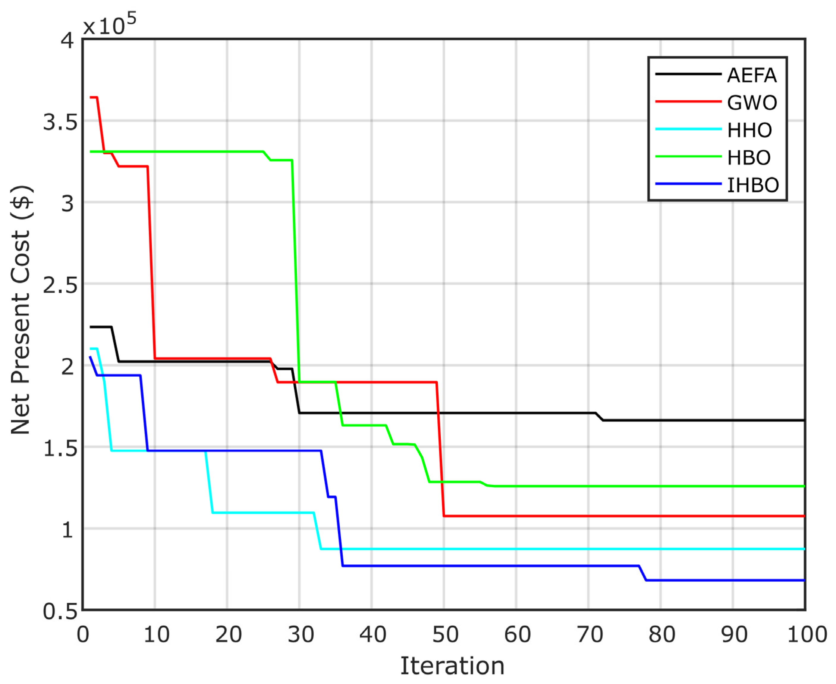
IHBO	165,999	0.1336	0.0445	99.9133	99.0391

, the results respect the constraints; then, the best algorithms results converge as HBO, GWO, AEFA, HHO, and IHBO, with an investment cost of MAD 461,233, MAD 226,559, MAD 221,694, MAD 215,371, and MAD 100,337, respectively. The best cost needs MAD 100,337, equivalent to MAD 0.08/kWh; in this situation, the LPSP is about 4%, the renewable fraction is near 100%, and the power availability is more than 99%.

Table 9. Sizing results of the PV/wind/diesel/battery HRES.

Algorithm	PV (m2)	Wind (m2)	Battery (kWh)	Diesel (kW)
AEFA	92.9	659.8	0.14	4.83
GWO	143.9	174	14.64	7.24
HHO	317.8	232.6	3.59	1.47
HBO	403.9	652.8	2.35	10.6
IHBO	261.3	102.7	23.2	1

presents the size results, which show that the best project needs 261.3031 m² of PV area, 102.7114 m² of swept area of the wind turbines, 23.2177 kWh of battery, and 1.0762 kW of diesel.

Table 10. Convergence time of the algorithms.

Algorithm	Convergence Time (s)
AEFA	1176
GWO	1079
HHO	3931
HBO	680
IHBO	4942

presents the convergence time of all simulations.

Figure 17 presents the convergence curve of the NPC for the PV/wind/diesel/battery HRES; the curve shows that the IHBO algorithm gives better convergence results.

6.2. Impact of Fuel Price Variation

In the paper, if we suppose that the price of fuel is about MAD 0.41/L, then we can compare the total investment cost with the previous study that used the actual price, which is MAD 0.96/L.

From

Table 11. Results of the PV/diesel/battery HRES with fuel prices.

Algorithm	NPC (MAD)	LCOE (MAD/kWh)	LPSP	RF (%)	Availability (%)
AEFA	166,303	0.1339	0.0324	96.1598	99.4268
GWO	107,532	0.0865	0.0483	97.0846	98.0032
HHO	87,394	0.0703	0.0496	99.6090	96.1823
HBO	125,791	0.1012	0.0296	97.7468	98.8978
IHBO	68,121	0.0548	0.1119	99.9999	88.8055

, it is clearly shown that the NPC of the HRES is reduced strongly while it is passed from MAD 120,463.

Table 12. Sizing results of the PV/diesel/battery HRES.

Algorithm	PV (m2)	Battery (kWh)	Diesel (kW)
AEFA	216.7	3.7	6
GWO	163.7	0.4	2.24
HHO	161.8	0.7	0.29
HBO	194	0	2.79
IHBO	124.9	0	0

presents the optimal HRES size using all optimization algorithms. Figure 18 presents the convergence curve of the NPC for the PV/diesel/battery HRES, with a fuel price of MAD 0.54/L. This figure shows that the IHBO algorithm gives the better convergence results.

7. Conclusions

This paper proposed a platform to design an HRES microgrid system based on two configurations, PV/diesel/battery, and PV/wind/diesel/battery. The platform is based on modeling, power management, and a cost optimization study using an improved IHBO algorithm. The proposed IHBO algorithm proved its efficacy in finding the optimal solution compared with many algorithms, including AEFA, GWO, HHO, and the original HBO. In the paper, we discussed the case of reducing fuel prices and its impact on the investment cost. The results show that the NPC is highly reduced when the use of diesel is small. Several systems, such as hydrogen storage and biomass systems, can be integrated in the microgrid. Future work will focus on developing configurations considering the degradation of battery characteristics.