1. Introduction
In the railway industry, safety has always been prioritized against other variables [
1,
2]. Nowadays, maximum levels of safety are guaranteed by the state-of-art. For example, signalling systems continue increasing their safety levels, avoiding human errors, and reducing potential risks [
3]. From the operator’s point of view, it is also important to optimize and reach high values of reliability, availability, and maintainability of the principal train components. In that sense, less interventions will be needed, less incidences will occur during commercial services, and no deviation for the rail service planned scheduling should emerge. These concepts are directly related with the technical part of the train, but not with the interphase between the final users and the operator. For this reason, another very important concept arises: user experience and passenger comfort.
Since the beginning, the main goal of the different means of transport was transporting people or goods from one place to another. Passenger expectations were limited to acquiring this basic service. Due to technological progress, a more complete service has been offered to the final users, with a consequent increase in the expectations and requirements from the passengers. In the last few years, user experience has emerged as a new concept because passengers are demanding not only a mere trip, but also a memorable experience.
In relation to passengers’ satisfactory experience in the train, it is also essential to offer a very high degree of comfortability, avoiding train wobbles or sudden movements. Many sensors and electronics are being used to supervise railway dynamics and infrastructures [
4], focusing on safety assurance and contributing to the condition-based maintenance topic. Generally, the three main reasons that cause a feeling of comfort loss in passengers are: punctual track irregularities that generate acceleration peaks [
5], a non-optimized guidance of the train that can cause a constant loss of comfort over time [
6], and the malfunctioning of any of the components implicated in the dynamic behaviour of the train (damping and suspension) that can also cause an extended loss of comfort. The implemented methodology in this study is focused on the second and third cases because it intends to detect lack of comfort that can lead to an uncomfortable experience for passengers. These cases can also derive in potential failures of suspension and damping components, so their early detection is essential to create a predictive maintenance strategy.
In this paper, an artificial neural network model is developed with the aim of detecting comfort degradation in the train, with the lateral car-body acceleration as a target variable to be predicted. The prediction is based on the interrelation between all the accelerations measured in each instant of time: lateral and vertical car-body accelerations, lateral wheelset accelerations, and the train’s overall speed. Based on these variables, the algorithm is trained to characterise the good behaviour of the car-body accelerations (high quality comfort) using real data obtained from healthy trains (with no damping or suspension damaged or worn components). A comfort loss or damaged component is detected once the difference between the real value of lateral car-body acceleration and the predicted value for this acceleration becomes noticeable.
In the state-of-the-art, there are many studies that achieve excellent results in predicting the accelerations of the train’s coaches. In fact, some of them use advanced predictive algorithms such as neural networks and statistical correlations to predict this variable [
7,
8]. In addition, other studies address the prediction of comfort values in high-speed trains using multibody dynamic models, including information about the track geometry and a simplified model of the rolling stock [
9,
10]. However, there is not any study that merges these two ideas together in a mathematical and engineering sense. The intention of this study is to address the prediction of the lateral car-body acceleration in a high-speed train using a neural network for the following purpose: the implementation of a methodology that compares these predictions to the real values measured on the train in order to obtain a continuous monitorization of comfort status in the train. Testing this methodology with a real case of application achieves a continuous onboard monitorization system of comfort degradation. The norm EN12299 [
11] is validating ride comfort for passengers only once during the certification process of the train in case it is contractually required, but it is not offering a methodology for a continuous monitorization of the train ride comfort for passengers.
In this sense, the railway sector needs to continue evolving considering this new condition-based maintenance (CBM) concept, not only for maintenance cost optimization but also to improve passengers’ comfort and, therefore, user experience. The methodology and the results are useful to develop an on-board health monitoring system [
12,
13], with two main goals: contribute to a predictive and more sustainable maintenance strategy aligned with the CBM concept, and to improve the user experience concept, fulfilling passenger’s comfort expectations. The first objective will satisfy operators, manufacturers, and maintainers, as the maintenance concept has evolved from the traditional corrective maintenance to the predictive and prescriptive maintenance, which is still being developed as part of the CBM [
14]. The second objective will satisfy the entire railway sector, including the final users [
15].
The optimized model is an excellent contribution to the early detection of comfort degradation or any failure in the damping system that could cause speed limitation, or even the declaration of a useless train due to safety concerns. In this case, operators or manufacturers might incur high penalties for the delay produced. In addition to this, an optimization of resources is reached through the identification of anomalies and deficiency patterns in order to trigger alerts when a component is coming to the end of its life [
16].
Furthermore, the algorithm and methodology developed in this paper offers a key performance indicator (KPI) of the train comfort degradation measured in real time. This KPI fulfils two main objectives: identify the comfort loss in a very advanced phase before it is noticeable by the passengers, and predict an imminent failure mode of the train damping or suspension’s components. This prediction is based on the comparison between the predicted lateral acceleration values and the real time monitored values. If a deviation between both curves is detected and the difference is constantly increasing, then an early comfort loss is identified, or even a potential component failure is detected.
As a consequence, a good implementation of predictive maintenance is surely causing clear economic benefits and contributing to the sustainability of the whole maintenance process [
17,
18]. Newly, sustainable transportation is becoming a key issue to reduce emissions and to address energetic efficiency that leads to a lower environmental impact.
2. Theoretical and Mathematical Foundations
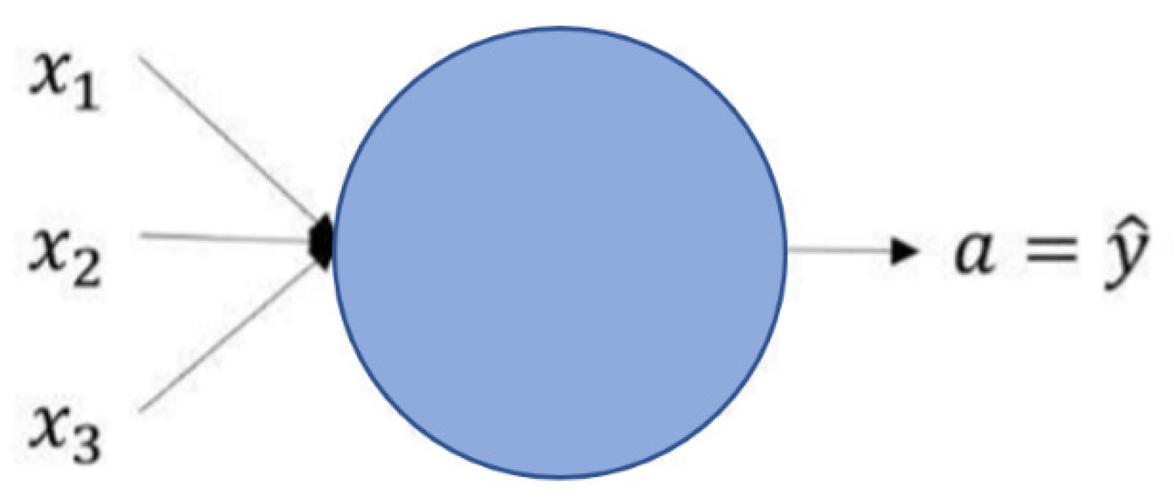
An Artificial Neural Network (ANN) is an iterative computer model commonly used in Machine Learning applications that learns certain behaviours, patterns, or relationships (especially non-linear relationships) from given data, and uses that knowledge to make predictions. Generally, ANNs are based on a set of simple, constructively identical nodes, called artificial neurons or perceptrons. These perceptrons are grouped in layers, so that all the perceptrons in one layer are connected to all the perceptrons in the next layer, allowing the transmission of information between layers of the ANN. Each neuron receives the values of the outputs (activations), computed by the neurons of the previous layer as an input. Equivalently, neurons compute the activation that will be sent to downstream neurons. Each neuron is characterised by the following trainable parameters:
wi (weight) and
b (independent term), as shown in the structure of an artificial neuron in
Figure 1.
In
Figure 1,
xi represents the
ith training sample that comes as an input to the neuron, and
a represents the output. The output of the last neuron of the neural net corresponds to the final predicted value for the
ith training sample.
The inputs or activations received are subjected firstly to a linear operation, and secondly to a non-linear operation. The linear operation can be expressed by:
where
represents the result of the linear operation,
represents the weight vector for the
ith training sample,
represents the output of the previous neuron taken as the input in this neuron, and
represents the bias value for that neuron.
The non-linear operation or activation phase is implemented, in this case using ReLU functions, and can be expressed by:
where the function
represents the ReLU function and
represents the output of that neuron.
As mentioned before, neurons are displayed within three types of layers: the input layer, hidden layers, and the output layer. The number of hidden layers in a neural network depends on the problem to be solved and is a hyper parameter of the model that must be optimized to maximize its accuracy. Setting a high number of layers makes a deeper and more complex neural network. The idea behind building an ANN model is that it can learn and extract intrinsic relationships from the provided data, being able to generalise the normal behaviour of the train and use that knowledge to predict accelerations and spot anomalies. In order to achieve this, the ANN learning process which is applied to the data (actually not the full dataset, only the training set) can be divided into different phases.
First, the model’s trainable parameters are randomly initialized with a standard normal random distribution of zero mean and unit variance. For better performance in this paper, He normal initializer is also applied [
19,
20], which is commonly used for ReLU activation functions. Once the model’s parameters are initialized, the data is introduced into the input layer of the artificial neural network and a random prediction (due to random initialization of parameters) is made after computing the operations in the neurons. The aim of the model is to get a better prediction after every iteration, as learning algorithms are generally based on iterative numerical methods that minimize the error of the predicted values. The error value is quantified through a cost function, which is the objective function of the computational model. The cost is computed by comparing the predictions to the real values (target values).
In order to update the trainable parameters of the model and keep reducing the error value, gradients of the cost function with respect of the variables are computed. Since the calculated gradient points are in the direction of maximum cost growth, the model parameters are updated, moving in the opposite direction of the gradient. This phase is called “gradient descent”, and parameters are updated based on the “backward propagation” algorithm [
21]. At the end, a numerical optimization method is used to estimate the best parameters to minimize the cost function. At this point, the model has succeeded in finding the parameters that result in the lowest error value, and, therefore, it could be said that the model is already trained and static (fine tune of the model is done later).
As mentioned before, the aim of this study is to predict the lateral car-body acceleration, which is the most representative variable to characterise the comfort status perceived by the passengers in the train. The reason for this is that lateral acceleration is the less controlled acceleration of the train: longitudinally, the train is guided by the previous coach, and vertically, the train is supported by the wheelset and secondary suspension. Therefore, lateral accelerations are directly perceived by the passengers as the vertical acceleration is partially mitigated by the floor and other components between the structure and the seats. For this purpose, the column (feature) of the lateral car-body acceleration will be predicted separately, and afterwards compared with the real values to check the performance of the model. Therefore, this corresponds to a regression task in which lateral car-body acceleration is predicted (target variable) attending to the other variables in the dataset (predictors).
The ANN training is performed by iterating over epochs until the model parameters converge to successful values. The function to be finally optimized is the cost function, which is defined in the next section as the sum of all the differences between the predicted value and the real value.
3. Data Preparation and Statistical Analysis
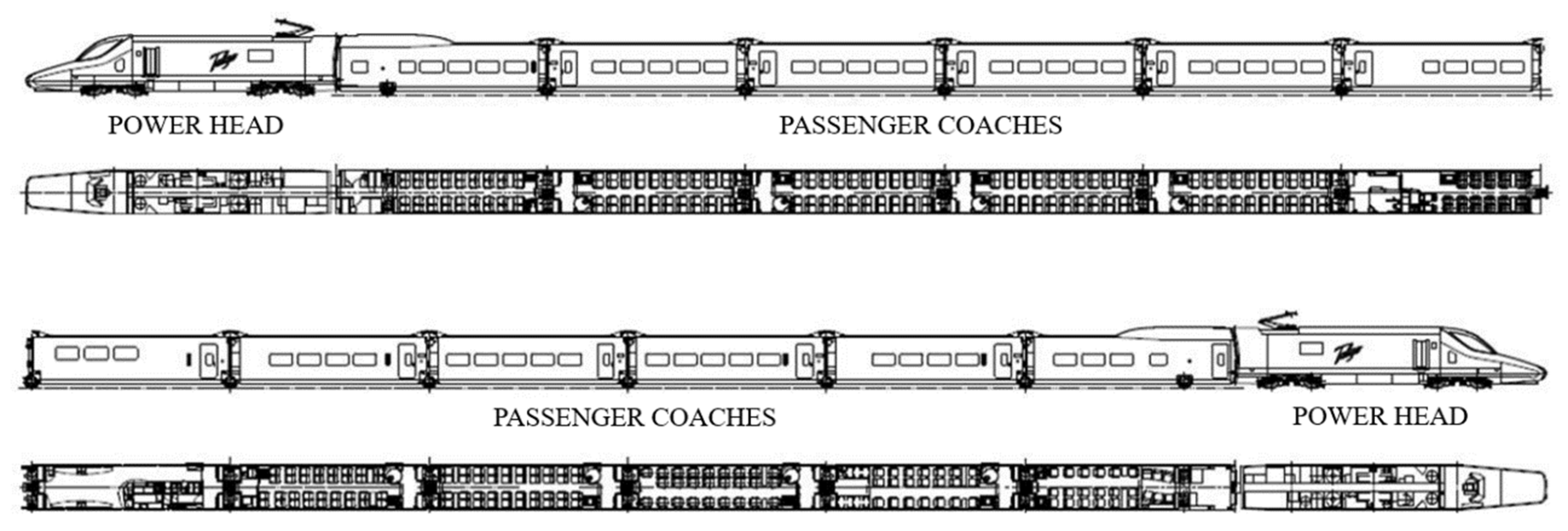
In this paper, existing data from a specific high-speed train model has been used. A dataset of one year is considered representative for this study, as enough samples are registered for a model optimization and all particular situations due to the fact that external conditions are contemplated in this period of time. The dataset corresponds to the year 2017. The selected type of train operates in lines at a maximum speed of 300 km/h. Madrid-Valencia is an example of these lines. This particular trainset is formed by two power heads and 12 passenger coaches, but includes 13 axles because the 6
th coach has a double axis as it is represented in
Figure 2. The maximum weight per axle is 22.5 t and the distance between them is 13.3 m.
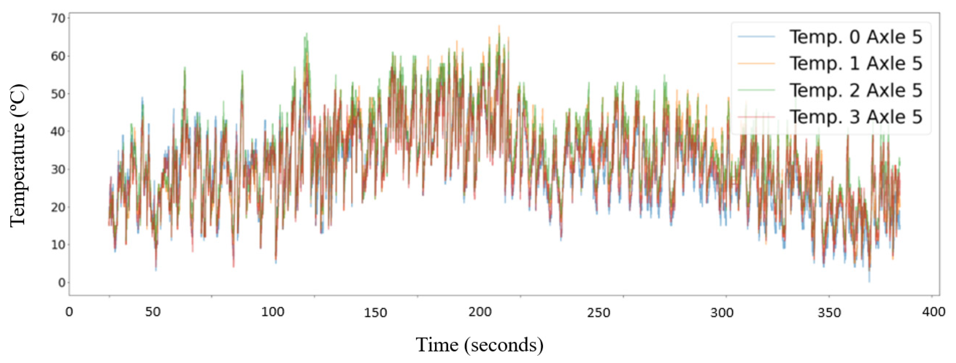
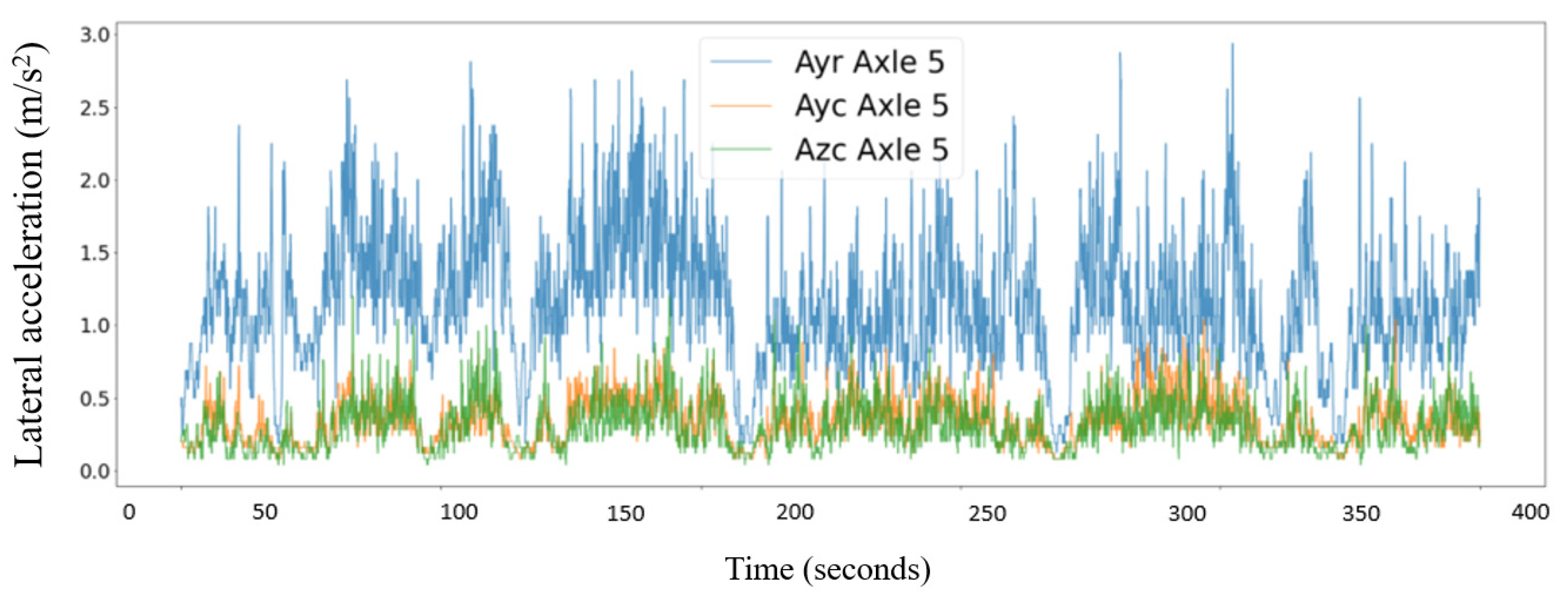
Many variables are registered in a high-speed train. Some of them are continuous signals, such as temperatures or accelerations, and others are state variables, such as the status of the pantograph (up or down). The dataset used in this study contains the following continuous variables recorded in real time: train speed (v), exterior temperature (Text), bearing temperatures (T0–T3 as there are 4 bearing temperature sensors per axle), braking pressure (p), lateral wheelset acceleration (Ayr), lateral car-body acceleration (Ayc), and vertical car-body acceleration (Azc) of all of the 12 coaches of the trainset.
In
Figure 3 and
Figure 4, the signal of bearings’ temperatures and accelerations are plotted for axle 5 as an illustration of these features’ behaviour.
Each row of the dataset contains the values of the mentioned variables measured by the sensors in one instant of time (one second).
In the case of the accelerations, it is important to highlight that the recorded values are statistical values calculated as the root mean square values over 5-s intervals of frequency-weighted accelerations according to the norm EN12299 [
17]. The train is equipped with 12 car-body accelerometers (one in each coach) that record lateral (Ayc) and vertical (Azc) car-body accelerations. In the case of the wheelset, there are 2 accelerometers per axle, so a total amount of 34 accelerometers are installed in the train (13 axles in the coaches and 8 accelerometers in the power head bogies) that measure the lateral wheelset acceleration values (Ayr).
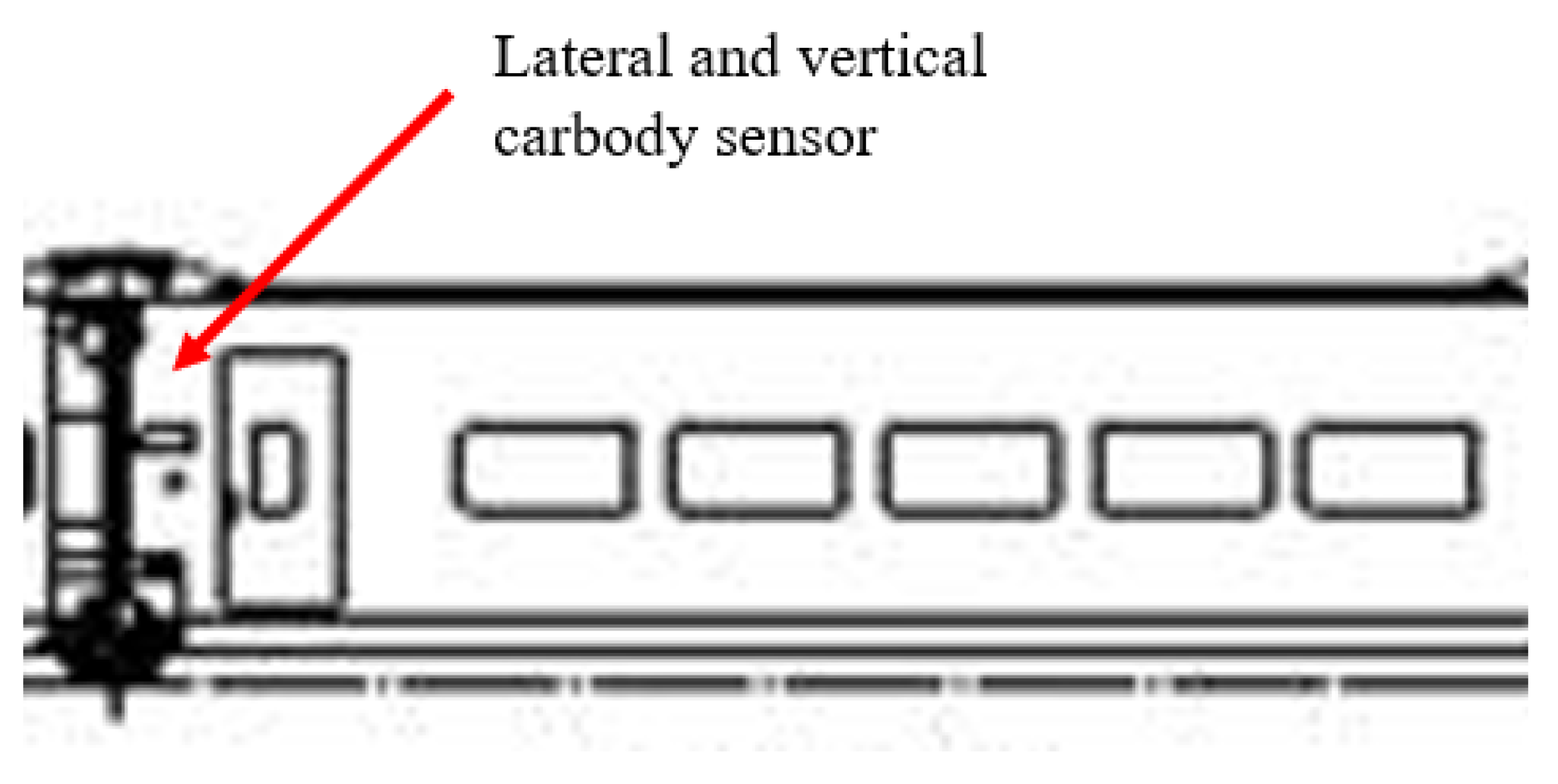
Figure 5 represents the position of the acceleration sensors of the car-body. These sensors are placed in the upper part of the endwall of the coaches due to the easy accessibility of this component for maintenance replacement or inspection. These sensors are accessible through the exterior door mechanism in the left part, as indicated in
Figure 5. The dimensions are approximately 100 × 35 mm, and the rolling lateral acceleration sensor is placed in the central part of the frame of the wheelset. The wheelsets are always located between two coaches.
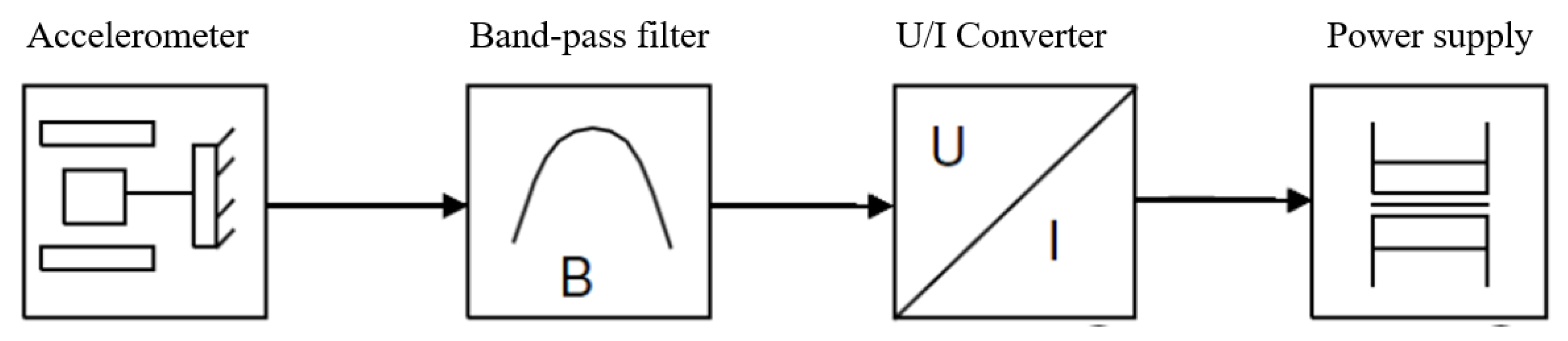
The sensors are composed by one accelerometer, one band-pass filter (>24 dB/octave), a U/I converter, and a power supply. The configuration of the sensor is presented in
Figure 6.
This configuration applies for the car-body and wheelset sensors. The only difference between both is that the car-body sensors are biaxial accelerometers (to measure lateral and vertical accelerations), and the wheelset sensor is uniaxial as only the lateral acceleration is measured. The frequency range of the band-pass filter is between 0.4 and 10 Hz. 4–10 Hz. Outside this band, there is an attenuation of 3 dB (70% of the signal), with a gradient of greater than 24 dB/octave, with a tolerance of ±0.5 dB within the band, and ±1 dB outside the band. It must be highlighted that synchronization of the sensors is assured as all the electronics that are recording the sensor’s measurements are connected to the TCMS (train control and management system).
In general terms, data registered by the sensors is reliable and robust. The more reliable the initial data, the more accurate the prediction model is. However, a pre-processing stage is done to handle outliers and detect sensor failures to eliminate this noise in the dataset. For this data preparation, it is also important to determine the most relevant variables to characterise the lateral car-body acceleration, which is the main purpose of this paper. Additionally, variables that are not influencing the dynamic behaviour of the train could be eliminated from the dataset in order to reduce the dimensionality of the dataset, making the optimization process of the neural network more efficient. For this purpose, a principal component analysis (PCA) is applied to the dataset. The PCA is a statistical technique to reduce the dimensionality of a dataset and determine the most relevant variables that are explaining the dataset. It is very useful in situations where large multivariate datasets are analysed.
With this technique, two principal directions are determined as linear combinations of the original data. These directions contain the most relevant information (explained variance) of the dataset. Then, original data is projected in these two principal directions to analyse the correlation between those variables graphically.
As shown in
Figure 7, dynamic variables (speed and accelerations) are plotted close to each other, indicating the high correlation existing between them, whereas temperatures are plotted across the opposite direction. This is a strong indicator of the physical independence between these features. The dynamic behaviour of the train is mainly explained in the principal direction 2, due to the accelerations and speed of the train. The thermal behaviour is explained in the principal direction 1, due to all of the temperature variables registered. As a conclusion, thermal variables are discarded from the dataset, as they provide no essential information and slow down the training phase. It has been verified that including these thermal features does not improve results. As a result, in the final model of this paper, only speed and accelerations are included.
Once the data has been cleaned, the second step is to consider only data corresponding to a train speed higher than 50 km/h, because comfort degradation is mainly noticed at high speeds. Since the goal of this study is to obtain a model to learn and characterise the correct behaviour of high-speed trains in terms of comfort, it is necessary to ensure that the dataset used to train the neural network does not include samples corresponding to lack of comfort situations; however, neural networks are quite robust to outliers. In order to get the correct dataset, information regarding the anomalies (comfort loss due to excessive accelerations) suffered by the train during 2017 was collecte d. According to expert opinion, the samples corresponding to 15 days before the anomaly detection date were removed from the dataset. Thus, the model is inferring knowledge about good functionality of the train, and it is capable of successfully predicting this kind of situation. Hence, when the neural network predicts accelerations with high error compared to the sensor’s measure, it is indicative of potential suspension or damping component failures. This is the process behind the need of predicting correct lateral accelerations to detect comfort degradation.
4. Model Definition Process
In regression applications where the principal goal is the prediction of concrete values in a continuous distribution, the absolute error is commonly used to measure the cost of each iteration, expressed as:
. The cost function to train the model is defined, finally, as the mean absolute error (MAE):
where
represents the value for the mean absolute error (MAE),
represents the weight matrix,
represents the bias vector,
represents the number of samples in the training set (number of rows), and
represents the cost of an iteration between the real values
and the predicted values
.
To avoid overfitting, which is a phenomenon that occurs in automatic learning algorithms as a result of excessive training on a set of data with known results, the tendency of the model is forced to reduce the value of the weights adding a summation in the cost function. This is called regularization:
where
represents the regularization parameter, which is a hyperparameter, and
represents the total number of layers in the neural network.
In this paper, L2 regularization method has been used [
22]. Having defined the cost function of the model (MAE) and the regularization type, the model can be trained. In each iteration of the training phase, the trainable parameters of the ANN (
w and
b) are updated in the negative direction of the gradient in order to minimize the cost. To compute this gradient, it is necessary to obtain the derivatives of the cost function with respect to each trainable parameter, which are computed using the gradient descent and backpropagation algorithm [
21]. Thanks to these algorithms, it is possible to efficiently reach the minimum of the cost function and succeed in the training phase. For the backpropagation phase, multiple methods and optimizers are defined. In this paper, the Adam optimizer (Adaptive Moment Estimation) [
23] has been implemented in order to decrease the training time of the model and improve its performance.
For the implementation of an ANN, it is necessary to divide the whole dataset into three sets:
Training set: used to train the ANN.
Validation set: allows the optimization of the hyper parameters of the model. Before reaching the final model, different models are analysed, so the results on this set will determine the most effective model.
Test set: the target variable (in this case lateral car-body acceleration) is removed from the test set and is used as a variable containing labels: the actual desired values. The aim of this test set is to verify that the model chosen from the validation set could be generalised to completely independent data from those used to design and evaluate the final model.
To evaluate the performance of each model, three performance metrics are defined:
Mean Absolute Error: a mean absolute error around 3% of the typical maximum estimated values for acceleration in the vehicle body is reflected in the EN14363 for the passenger coaches (1.5 m/s2), which means 0.05 m/s2 will be considered a successful result after expert consultation.
Maximum error: a maximum error between the predicted values and the labels (real values) is less than 20% of the typical maximum estimated values for accelerations in vehicle body reflected in the EN14363 for the passenger coaches (1.5 m/s2), which means 0.3 m/s2 will be considered a successful result.
Overflow error counter: this metric measures the percentage of data predicted with an error greater than 0.25 m/s2. It is important to check that there is no excessive deviation of the error, so the reliability of the model is appropriate for its purpose. If less than 1% of the data exceeds 0.25 m/s2 (15% of the typical maximum estimated values for accelerations in vehicle body reflected in the EN14363 for the passenger coaches (1.5 m/s2), it will be considered a successful result.
5. ANN Models and Results
In this paper, some models have been defined with upward difficulty to compare their results and determine the most appropriate model for this real application: the prediction of lateral car-body accelerations to avoid comfort degradation and detect damping or suspension deficiencies before a service breakdown is produced. This variable is the most representative in terms of comfort (because it is directly affecting to the passengers) and failure detection in the damping or suspension system, as it is the end of the force transmission chain after the secondary suspension. It is also the variable with the highest degree of freedom.
After the data pre-processing phase described above, the remaining set has 200,000 samples used to train the neural network. In the pre-processing phase, non-reliable data and error data are removed, and data corresponding to speeds under 50 km/h are deleted as well. As previously stated in the paper, the dataset corresponds to a high-speed composition containing variables recorded every second during the year 2017. Each sample, after the cleaning up of the dataset, includes the following variables: lateral car-body acceleration (Ayc), vertical car-body acceleration (Azc), train speed (v), and lateral wheelset acceleration (Ayr) for all of the 12 coaches of the trainset. There is a total number of 40 variables (Ayc, Azc, and Ayr in each of the 13 axles of the coaches and the train speed). The target variable is the lateral car-body acceleration (Ayc) and the predictor variables are the speed (v), the vertical car-body acceleration (Azc), and the lateral wheelset acceleration (Ayr). The input matrix X for the neural network is a (200,000; 40) dimensional matrix, and the vector containing the true values Y (used to compute the cost in each iteration) is a (200,000; 1) dimensional vector. The X columns contain the variables described above for each coach.
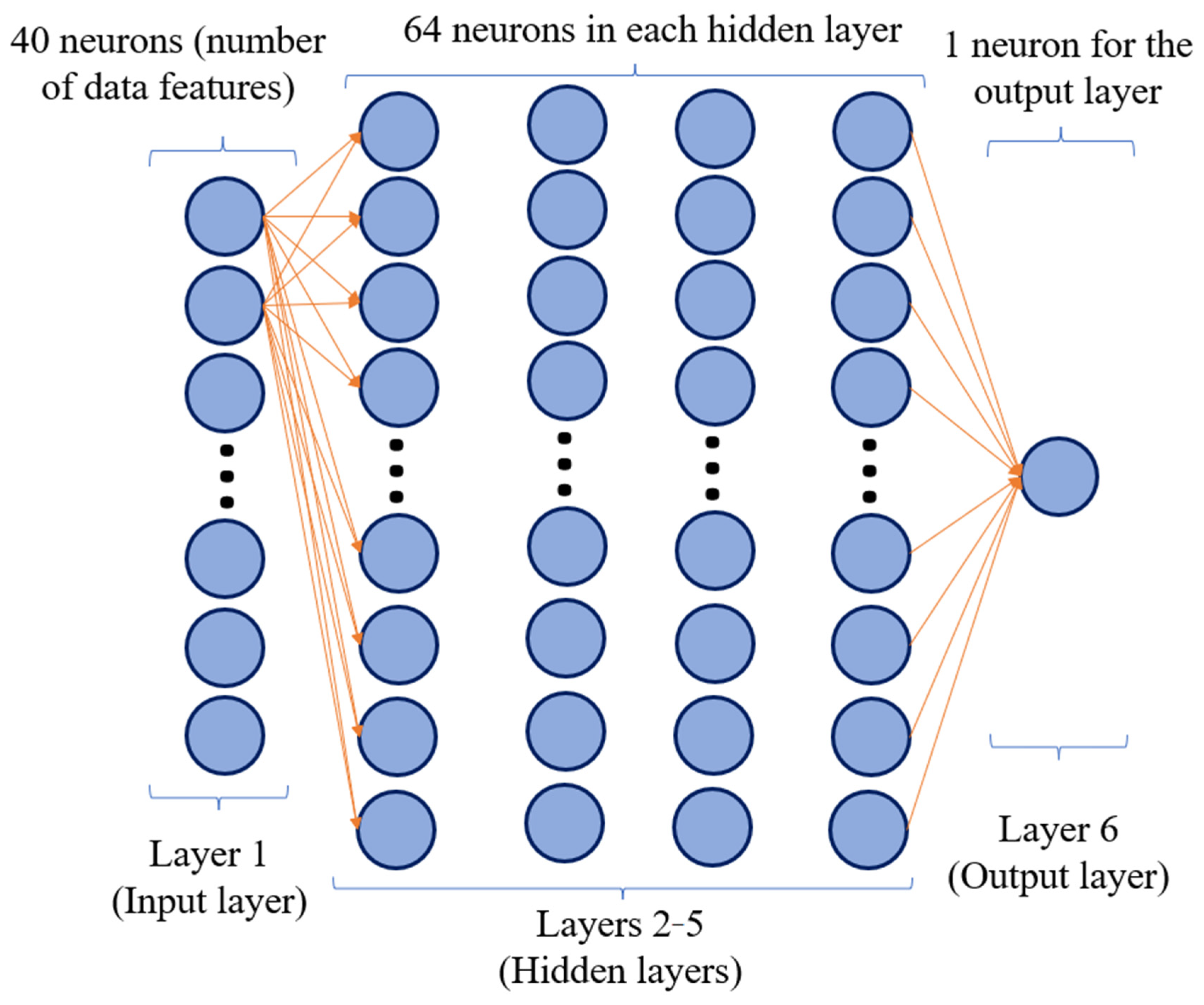
Before starting the training phase of the model, it is necessary to divide the dataset into three sets: training, validation, and test set. For this division, it should be considered that consecutive samples of the dataset could measure a very similar train status (acceleration values of all the coaches). A random choice of the three sets (just shuffling the dataset) would cause the separation of consecutive samples with the same acceleration values in different sets. This leads to overfitting of the model and derives in misleading results, as the model would memorize that sample but not generalise an actual behaviour. In consequence, the three sets are separated by months so there are no repeated samples in the training and validation/test sets. Moreover, 80% of the samples are used for the training set, 10% for the validation set, and the remaining 10% for the test set. After several experiments testing different architectures in the validation set of the neural network (changing hyperparameters), the final architecture defined for the model is formed by six layers (one input layer, four hidden layers, and one output layer), and 64 neurons per hidden layer.
A diagram of the neural network architecture is shown in
Figure 8. As mentioned above, the neurons of every layer are fully connected through the whole architecture; however, only a few connections are shown in the figure to make it more understandable.
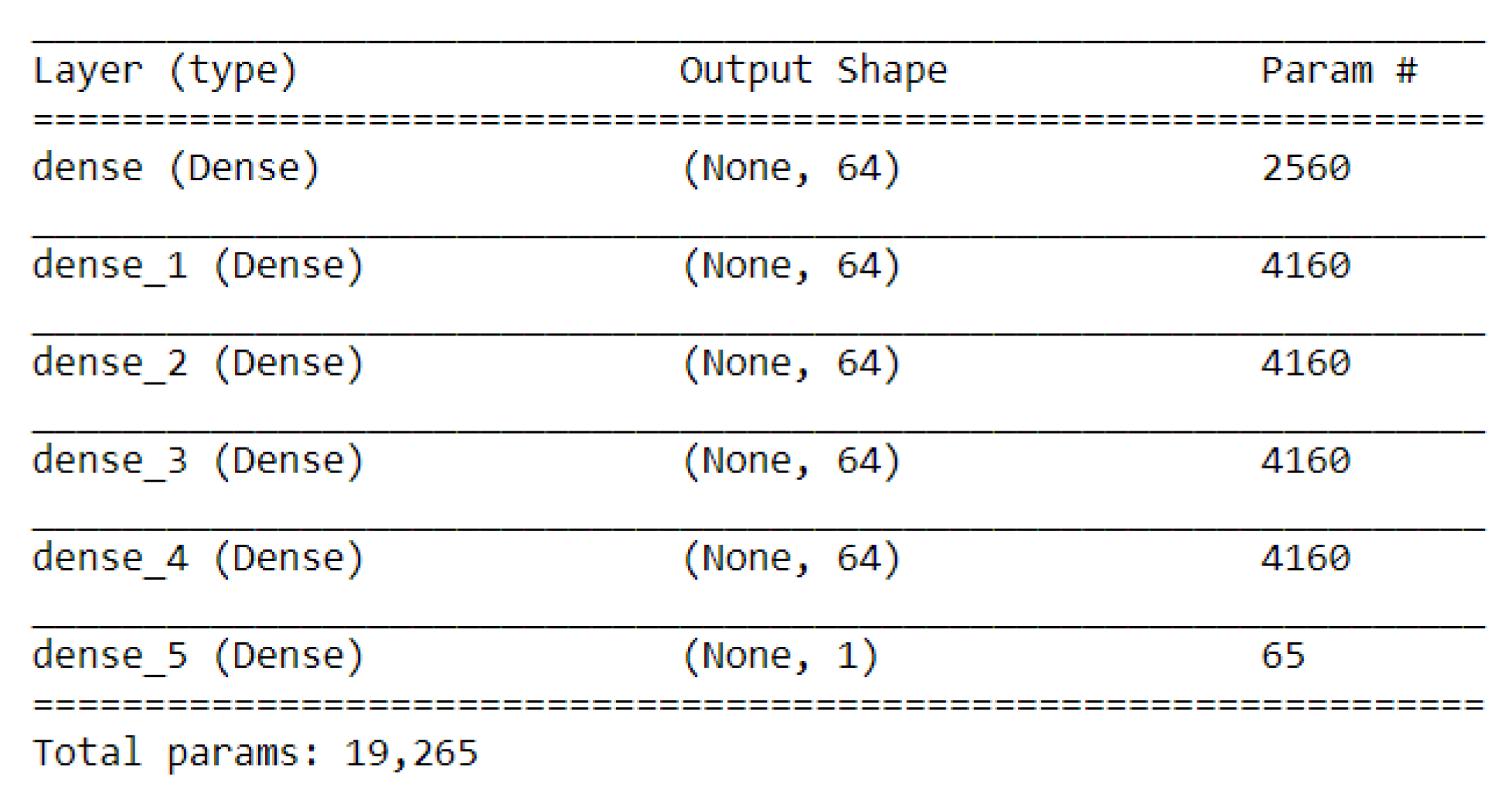
Overall, the model has 19,265 trainable parameters (
w and
b). Apart from the architecture, other parameters are set before the training phase starts. These are called hyperparameters. In this study, the tuned hyperparameters have been the learning rate and the regularization parameter. The learning rate has been set to 0.001, and the regularization parameter to 0.0001.
Figure 9 shows the number of trainable parameters in each layer in the final model.
The reason why the model has only six layers and 64 neurons is because making the architecture of the neural network more complex (increasing number of neurons and layers) leads to undesirable overfitting. In the obtained model, the lateral car-body acceleration of one axle is predicted using the information of the other axles. Thus, one model per train axle is needed. However, the architecture of the network and hyperparameters remains untouched for the different models.
To ensure that the trained models are good enough to solve the regression task of predicting the lateral car-body acceleration with new data, they are evaluated on the test set using the metrics that were defined before. The results of the test set evaluation are shown in
Table 1. The neural network takes around 80 iterations (epochs) to converge.
Table 1 shows that, overall, the acceleration is predicted with a mean absolute error of approximately 0.03 m/s
2 and a maximum error of approximately 0.4 m/s
2, which are considered excellent results. In addition, the number of samples predicted a mean absolute error of less than 0.25 m/s
2, which represents the 15% of the maximum estimated values for accelerations in vehicle body indicated in the EN14363 standard. It should be noted that for axles 1 and 13, the metrics are slightly poorer. This result is expected as the end coaches are directly connected to the power heads of the train, so the mechanical guidance and connection is not as robust as between the intermediate coaches. In consequence, the lateral movement is higher and, therefore, less predictable. However, results for axles 1 and 13 are within expected and accepted range as the error for these axles means 5.3% of the typical maximum estimated values for accelerations in vehicle body reflected in the EN 14363 for the passenger coaches (1.5 m/s
2).
In conclusion, the error margins obtained in the predictions are practically unnoticeable for the passengers in the train. This means that the algorithm is capable of detecting comfort degradation once the predictions are compared to the measured values by the acceleration sensors.
6. Model Performance in a Real Case of Application
At this stage, the optimized neural network is trained, which means its trainable parameters are static and predictions can be made by feedforwarding new information into the model. As shown before, the model achieves competitive results.
This neural network can be considered a CBM model because it is possible to achieve a constant monitorization of the accelerations in order to foresee a potential failure in the suspension and damping components.
The neural network model characterises the normal behaviour of the lateral car-body accelerations. For this reason, it is necessary to check the model’s performance on data containing samples corresponding to normal dynamic behaviour and other samples corresponding to comfort degraded behaviour (high lateral acceleration values). Theoretically, the model should not predict accelerations corresponding to train comfort degradation with the same accuracy as it does for normal accelerations. In order to prove this idea, a completely new dataset is introduced into the neural network, and the prediction results are evaluated. This new dataset contains around 10,000 samples and the same variables as before (train speed and accelerations for each axle), but it corresponds to a different year than the one used for training. This data was recorded in 2019, when a passenger sitting on the 11th coach of the train noticed an excessive lateral car-body displacement during his trip, causing a loss of comfort. As the typical maximum estimated values for accelerations in vehicle body reflected in the EN 14363 for the passenger coaches (1.5 m/s2) was far from being reached, the safety alerts were not triggered. However, a clear comfort degradation was detected, and a specific maintenance inspection was programmed to check damping and suspension elements of this coach. Indeed, one damper had to be replaced, so a technical reason for this situation was discovered.
The results obtained after predicting the lateral car-body accelerations for this specific dataset are shown in
Table 2.
As it is stated in
Table 2, predictions are extremely accurate for accelerations corresponding to axles 1 to 9. This means that those axles are within the expected range of lateral acceleration values corresponding to normal behaviour, so the model performs correctly. However, for axles 10 to 13, predictions are extremely poor. The model has a mean absolute error of around 0.4 m/s
2 in the predicted accelerations for those axles, and it foresees more than 60% of the data with an error greater than 0.25 m/s
2 (15% of the typical maximum estimated values for accelerations in vehicle body reflected in the EN 14363 for the passenger coaches (1.5 m/s
2)). Considering that comfort degradation was detected in the 11th coach of the train (leans over axles 10 and 11), the model is validated as the results perfectly describe the situation.
This is a clear example of a situation in which a comfort loss that derived in a damaged component and its replacement was not detected by the current system. Results have proved that if this model was implemented, the potential damage could have been foreseen and the system could have been correctly adjusted instead of directly being replaced. This model can, therefore, extend the service life of some components in the train and contribute to creating a more sustainable line of maintenance. Moreover, the implementation of this model in the train will enable the monitorization of the difference between the measured lateral acceleration values and the predictions of the neural network. A feasible CBM model is then achieved for this train series.
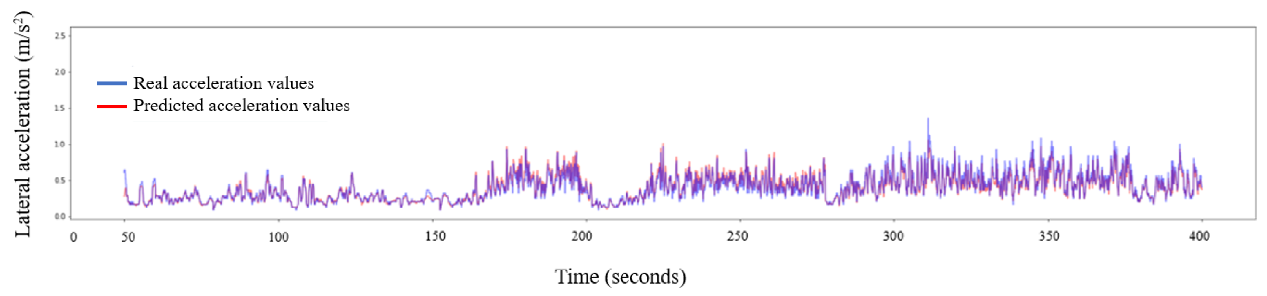
In
Figure 10, lateral car-body predicted accelerations and real accelerations of axle number 5 are plotted: the real values are represented in blue, and predicted values are represented in red. No relevant differences between the prediction and the real values are detected, so the model perfectly predicts good behaviour of axle number 5.
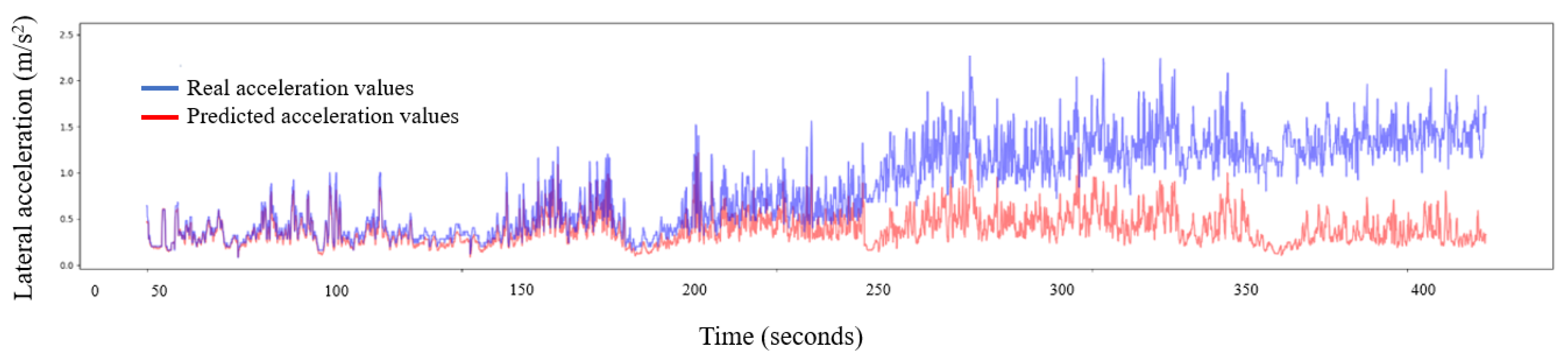
On the other hand, in
Figure 11, lateral car-body predicted accelerations and real accelerations of axle number 11 are plotted. A significant difference between the predicted values and the real values is detected, exceeding the established limits of normal behaviour of the lateral movement of the train. In this sense, a clear comfort degradation is detected in the same axle in which the passenger that alerted of the excessive lateral movement was seated.
The above defined model is focused on predicting lateral car-body acceleration of one coach considering the rest of the variables and the behaviour of the rest of the coaches. However, this predictive model can be extrapolated to other dynamic variable prediction (other accelerations or bearing temperatures, for example), reaching similar results and same satisfactory performance. In particular, it can be adapted to predict not only lateral car-body accelerations (Ayc) but also vertical accelerations (Azc), obtaining a mean training error of 0.029 m/s
2. Moreover, this model also is valid for the entire fleet. For other trainset models, minor adjustments should be implemented to assure the most optimized algorithm. The mentioned flexibility of the model to perform successfully in these situations is based on two factors: the neural network models’ robustness, and the similar technical characteristics of the dynamic behaviour of any train. On one hand, Artificial Neural Networks are one of the most robust Machine Learning algorithms when it comes to performing on similar tasks. This is because the regularization methods permit the algorithm not to overfit the data and reduce the variance of the model, allowing the neural network to generalise the dynamic behaviour of the train, but not only for this specific group of training data [
24]. In this paper, the L2 regularization method has been used to train the model, being flexible to slightly different data inputs [
25]. On the other hand, similarity between the dynamic behaviour of high-speed trains considering the same suspension and damping design concept makes the trained model applicable to other high-speed trains. The robustness and reliability of the data recorded to be used for training algorithms is fundamental for good model creation and optimization, so reliable electronics and sensors are required for obtaining optimized results.
7. Contribution to Sustainable Maintenance
This paper contributes with the evolution to a predictive maintenance and CBM concept and, consequently, to a more sustainable maintenance strategy of the railway systems. If most of the important failures during operation are avoided, and real-time monitored information is treated to adapt to the maintenance inspections required by the train, a clear optimization of the resources will be reached: preventive maintenance stops will be reduced, corrective operations will decrease, and extra displacements of the trains will be eliminated, reducing the use of energy, human, and material resources, and creating an energy efficient model. The state-of-the-art is creating the future idea of a sustainable maintenance model focused on a “none-maintenance” concept, where the train is responsible for visiting maintenance depots only when it is clearly needed, and in those cases where prescriptive or predictive maintenance are not able to definitively solve the detected problem.
Extrapolating this concept to the entire fleet, a global fleet train management architecture will assure this positive contribution to the social, environmental, and economic compromise aligned with the European objectives stated for 2030.
8. Conclusions
The main objective of this paper is reached: obtaining a CBM model through a neural network model capable of predicting the lateral car-body accelerations for the comfort degradation monitoring and the identification of damping or suspension potential failures. An optimized neural network and a demonstration of its satisfactory performance with a real case of application have been determined.
Firstly, comfort degradation monitoring is achieved in the sense that a real-time implementation of the neural network allows one to compare the predictions of the model (ideal behaviour) and the sensor measurements (real behaviour). In this way, it is possible to identify comfort losses if the difference between both values starts progressively increasing.
Secondly, potential failures in dynamic train components are identified as the neural network model predicts abnormal behaviour of lateral car-body accelerations. Frequently, abnormal accelerations respond to unusual behaviour of these components, so an inspection can be programmed preventively to avoid potential damages or to correct failures detected that could derive in higher damages during operation, such as loose screws or supports, worn fixations, damper’s oil degradation, etc.
Considering the technical implementation of the algorithm, an important fact is that training the model only taking into account the dynamic variables of the train is profitable. This implies reducing computing times, obtaining almost the same error rates; thus, a computational cost reduction is identified. This conclusion was also evidenced in the PCA statistical analysis.
The good performance of the model is demonstrated in two different results:
1->The mean absolute error obtained is 0.034 m/s2, which is less than 3% of the typical maximum estimated values for accelerations in vehicle body reflected in the EN 14363 for the passenger coaches (1.5 m/s2), which is considered a successful result.
2->The number of predictions with errors greater than 0.25 (as it is the 15% of the typical maximum estimated values for accelerations in vehicle body reflected in the EN 14363 for the passenger coaches (1.5 m/s2)) is quite low: 12 times in the training phase and 5 times in the test phase. Considering a total amount of 140,000 training samples and 30,000 test samples, approximately, in less than 1% of the samples, the limit is exceeded, acting as an important indicator for the good performance of the model.
However, further evidence of the success of the results is the real application case where the comfort degradation detected by a passenger was perfectly identified by the model: a mean absolute error of 0.6467 m/s2 and an overflow error counter of 75.1% far exceeded the proposed limits. Therefore, this model could be implemented in the context of condition-based maintenance: in case of detecting a deviation of normal behaviour, an alarm will be sent to the fleet management system. The meaning of this alarm is a comfort degradation detection or a potential failure of the suspension or damping system, so a specific maintenance stop could be programmed in advance to correct this situation before the incident occurs.
In summary, an optimal CBM model for detecting comfort degradation and premature suspension or damping system failures is obtained with successful results considering mean errors of less than 0.04 m/s2, which means unnoticeable values for passengers.
The state-of-the-art ensures safety in high-speed trains, but there is no constant monitorization of the comfort status in the train to assure the best comfort levels to passengers as proposed in this paper in order to contribute to user experience. This methodology is also aligned with a sustainable maintenance model considering the energy efficiency concept and the optimization of environmental resources.


 ,
, 


