
Optimal Loan Pricing for Agricultural Supply Chains from a Green Credit Perspective


Business School, Hunan Normal University, Changsha 410081, China
*
Author to whom correspondence should be addressed.
Sustainability 2021, 13(22), 12365; https://0-doi-org.brum.beds.ac.uk/10.3390/su132212365
Submission received: 15 August 2021
/
Revised: 30 October 2021
/
Accepted: 5 November 2021
/
Published: 10 November 2021
(This article belongs to the Special Issue Green and Sustainable Supply Chains)
Abstract
:In recent years, many countries have proposed various sustainable development strategies around environmental issues. The implementation of green supply chain management is an effective sustainable development approach that combines “environmental awareness” and “economic development.” Therefore, introducing the concept of “green” effectively is the main direction for the sustainable development of agriculture in the future. The impacts of green credit policies on agricultural supply chains have rarely been discussed before. Therefore, we focus on the incentive mechanism of green credit policies in the agricultural supply chain. We use the Stackelberg Leadership Model to construct a pricing model which adds the interest subsidy and required reserve ratio (RRR) cuts, and determines the pricing rules of bank loans and production decisions of the farmer in the agricultural supply chain under the incentive policy of green credit by quantifying the optimization problems of the bank and the farmer. The result shows that optimal decisions exist for both farmer and bank in the supply chain game framework. The implementation of the green credit policies contributes to both of their profits. Additionally, the green credit policies give the bank room to reduce interest rates so that the overall utility level of the supply chain could be improved.
1. Introduction
As a large agricultural producer, agriculture is a basic industry for the construction and development of China’s national economy. Rural financial markets have long been plagued by financial absenteeism and inadequate supply, resulting in lagging rural economic development and widening urban-rural income gaps. Studies have found that the implementation of agricultural financial policies plays an important role in compensating for the distortions in the cross-sectoral flow of capital caused by the different degrees of financial frictions between sectors [1], as well as helping farm households to escape from poverty [2]. At the same time, relying solely on public finance policies to support agriculture cannot play its proper role, and the combination of public finance and commercial finance is the key to building a sustainable rural financial system [3]. Therefore, guiding the financial sector through policies to help agricultural development is an important tool for the rapid development of rural financial markets. Modern agricultural production is a subject of supply chains involving multiple subjects in the industrial chain, and in this context agricultural supply chain finance becomes an important innovative force to break the rural financial market settlement and plays a positive role in poverty alleviation [4].
It can be seen that policy support and modern supply chain management play great roles in promoting the development of agriculture. Green credit policy (GCP), one of the supportive policies vigorously promoted by the government, is designed for environmental protection and sustainable development. Therefore, we focus on the impact of green credit policy on the profits of the farmer and the bank, which are both decision makers in the supply chain. We investigate optimal strategies of each subject under the green agricultural supply chain through the Stackelberg model, explore the mechanism of the impact of green credit on the whole agricultural supply chain and the optimization path to promote the benign development of the agricultural supply chain.
Our novelties and contributions are as follows. First, previous studies on green credit have mostly focused on macro level, but we study the influence mechanism of green credit from a micro perspective. We introduce green credit to the traditional agricultural supply chain to study the impact of green credit policies on green supply chain. Second, previous studies on agricultural supply chains are mainly about production and risk. We introduce green credit policy into traditional agricultural supply chains to broaden their research content. Third, previous studies on supply chain finance did not consider the randomness of output, but the output of agricultural products is stochastic because of climate change and natural disasters. We consider the characteristics of agricultural production and the randomness of output, which also makes our research more relevant to real world conditions.
2. Literature Review
The literature studies on green credit policy (GCP) are mainly related to the impact of green finance on building development, river and lake construction and marine economic areas, but there is a lack of studies on the agricultural sector [5,6,7]. Scholars have mostly studied the impact of green finance on industry and regional economies from a macro perspective. Some scholars have analyzed the current situation of green finance as well as the existing problems [8,9]. The problems of backward development of green finance in Hebei was found to include the lack of effective incentive policies, narrow financing channels and high financing costs in traditional industries [10]. Forest area, wastewater emissions, energy consumption, investment in environmental management and industrial structure can significantly increase the demand for green finance in eastern China [11]. The green credit effect was calculated in the Data Envelopment Analysis (DEA) model [12]. There is a non-linear characteristic in the economic growth effect of green finance, and the effect is scalable [13].
Some studies focus on aspects, such as performance evaluation and risk management of green finance. A green finance risk evaluation index system was constructed for China, taking into account the government, market and capital supply and demand [14]. One study added non-financial and green financial indicators to improve the performance evaluation system [15]. Another study analyzed that the risk of loss for green finance investment projects can be reduced by constructing a multi-party game model of the government, financial institutions and green enterprises [16].
Green finance and growth has also been studied for its environmental impacts. Green finance policy was found to inhibit polluting industries while promoting environmentally conscious industries with a greater impact in eastern versus western China [17]. Directions of green growth pathways were influenced by differences in inherent technical incentives in carbon reduction policies under carbon markets, carbon taxes and hybrid policies [18].
In terms of research methods, scholars have mostly used empirical models for macro data. Green factors can be incorporated into the traditional macro model [19]. Some scholars use the Computable General Equilibrium (CGE) model to study the systemic effects of green credit policies [20,21,22,23]. The Dynamic Stochastic General Equilibrium (DSGE) model can be used to study problems in green finance-related areas [24]. The traditional DSGE model has been improved to determine the mechanisms and effects of green credit incentive policies [25].
The literature on green supply chain management and finance is relatively well established. Some researchers have studied the social impact of green supply chain management. Green supply chain management has been found to have a positive multiplier effect on environment issues [26]. In a structural equations modeling study involving 159 manufacturers, green supply chain management practices were found to synergistically improve operational performance and economics while reducing environmental impacts [27]. A prior study on financing strategies in green supply chains concluded that green supply chain finance is an important force to help enterprises complete the paradigm shift and promote sustainable development [28]. Past research on the environmental performance of 58 microfinance institutions in Europe found that the scale of investment by non-banking financial institutions was closely related to the total environmental performance of society [29].
The business strategies of companies in the supply chain are also the focus of study. In green product supply chains where manufacturers are financially constrained, retailers should participate in manufacturer financing by adopting the early payment discount of zero financing strategy [30]. The manufacturer prefers to purchase from low-cost green enterprises with less risk, and the positive impact of green credit policy (GCP) on supplier performance is also more concentrated in low-cost enterprises [31].
From related studies of supply chain finance, we can see that fuzzy theory and game theory models are widely used in pricing strategies. The Stackelberg game model was used to analyze the pricing and greening strategies for a competitive dual-channel green supply chain under a uniform pricing strategy [32]. The one-population evolutionary game theory was used to discuss the pricing strategy and long-term actions of socially concerned producers [33]. The fuzzy theory was used to explore pricing of substitutable goods in a supply chain with a common retailer and two competitive producers [34]. By using game theory, the pricing policies for dual-channel supply chains with green investment and sales effort under uncertain demand were investigated [35]. Another study investigated the pricing and coordination issues of a two-echelon green supply chain system under both green and hybrid production modes [36].
The introduction of supply chains into agriculture began in the 1990s. In the beginning, a complete set of network and agricultural information decision support systems that were suitable for China’s situation were constructed [37]. Since then, Chinese scholars have studied many issues around the agricultural supply chain, such as farmers’ income under bank credit, the randomness of agricultural output and the risk protection of insurance for farmers [38,39,40]. In addition, scholars have also investigated online agricultural supply chain, risk evaluation, prevention and control of agricultural supply chains, performance evaluation and agricultural supply chains in the context of big data and blockchain [41,42,43,44,45].
These practices and previous studies indicate that green supply chain management is mainly focused on manufacturing industries, such as automotive, furniture, electrical and electronics and construction, but less on agriculture. Prior literature focuses mainly on the environmental and economic impacts of green supply chain implementation or the decision making of internal companies, but less on the impact of green incentives from external governments on the supply chain. The practice of green finance is also widespread, and there are many scholars who have studied the impact of green credit policies on industries from the perspective of policy effects. However, most are macro-level empirical studies, and there is a lack of micro-level theoretical studies. As for agricultural supply chains, studies focus on output uncertainty, optimal decision making and risk management. However, there is less literature on the introduction of green credit on the basis of traditional agricultural supply chains and policy impacts on these types of supply chains. Furthermore, there is a lack of quantitative studies in particular on agricultural green supply chain finance. Therefore, against the background that China attaches great importance to agricultural development and the lack of relevant research, we introduce green finance to the traditional agricultural supply chain, investigate optimal strategies of each subject under the green agricultural supply chain through the Stackelberg model, investigate the impact of green credit policies on the green supply chain and propose corresponding policy recommendations.
3. Methods
3.1. The Basic Model
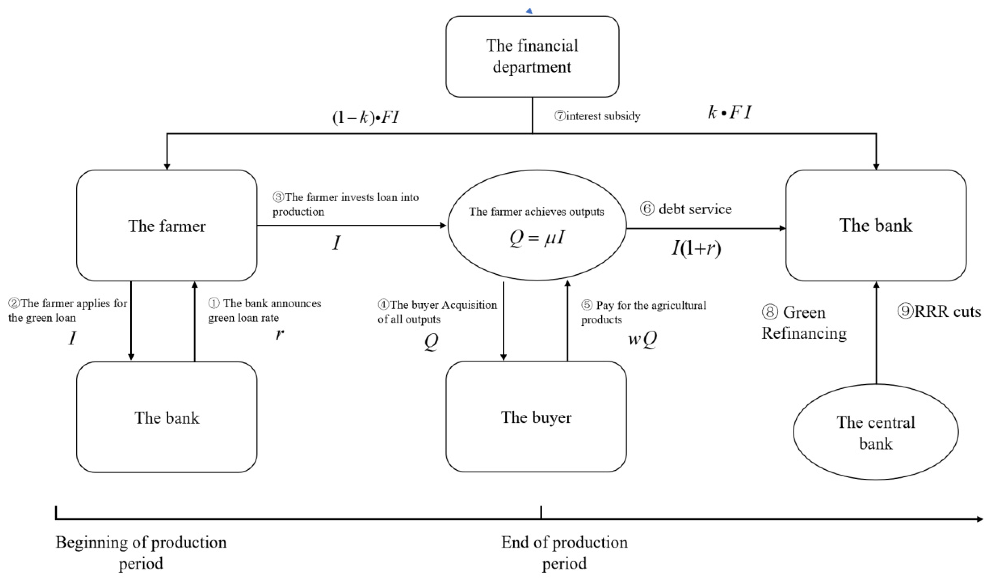
We considered an agricultural supply chain consisting of a representative farmer, a buyer of agricultural products and a bank that introduced green credit-related activities. In this supply chain, the bank as the leader and the farmer as the follower constitute a Stackelberg game model. The bank sets the green loan rate and the farmer chooses his own loan amount according to the bank’s rate. At the same time, the bank can predict the loan amount of the farmer and set the green loan rate based on it. The green loans can receive subsidized interest rates from the finance department and a certain degree of required reserve ratio (RRR) cuts from the central bank. The farmer takes out a mortgage with his fixed assets and starts to organize production after obtaining the loan. We assume that all production is financed by a green loan from the bank. At the end of the production period, the farmer sells all the agricultural products to the buyer.
At the beginning of the production period, the bank predicts the amount of the loan of the farmer and thus sets the green loan rate r where 0 < r < 1. The farmer observes the green loan interest rate and thus uses his fixed assets a as collateral to apply for a green loan from the bank in the amount of I. We divide the lending business of the bank into two types, green loans and non-green loans. We call the interest rate corresponding to the loans that the bank lends to the farmer for agricultural production the green loan interest rate, which is r. While other loans are non-green loans, and the corresponding interest rate is the non-green loan interest rate. After obtaining the financing, the farmer starts to produce agricultural products. We assume that the production process is affected by other factors, such as climate change and seasonal changes, so there is an uncertainty in the final yield of agricultural products. We use a random variable μ denoting the production efficiency, whose probability density function and distribution function are f(μ) and F(μ), respectively. The output of the farmer is expressed as Q = μ × I. At the end of the production period, the farmer sells all the agricultural products to the buyer in this supply chain. The buyer sells all the agricultural products in the market to maximize his profit.
For sales, we adopted the assumption that all agricultural products can achieve the equilibrium of supply and demand in the market at the price p [46]. We assume that the market demand of agricultural products D is elastic to the price p, and . denotes the choke price of agricultural products, it means that once the market price of the product is higher than the choke price, its demand becomes zero. k is the inverse of the price elasticity of demand, it describes the demand responsiveness to product price. We can get from the equation . When the product market is cleared, the market demand is equal to the total supply of agricultural products, that is D = Q. What is more, the buyer can purchase agricultural products at price w, which is lower than the market price p. We set w = m × p, where m denotes the bargaining power of the buyer, 0 < m < 1.
The bank we introduced is a bank that conducts green credit activities. We assumed that the bank operates deposit and loan business on a daily basis. The deposit business is to deposit for households and pay interest to households on their deposits, and the interest rate is . The loan business is divided into two categories: green loan business and non-green loan business. The volume of green loans is I, the interest rate on green loans is r, while the volume of non-green loans is and the corresponding rate is . The bank is required to pay statutory deposit reserve and excess deposit reserve as required by the central bank. As a result of green credit activities, the bank can get the green credit subsidy at q × F × I from the finance department, where F is the subsidy rate, q is the percentage of the subsidy that the bank gets. What is more, the bank can also get the central bank’s targeted RRR cuts based on green loan volume and green refinancing. The specific process is shown in Figure 1.
3.2. Optimal Strategy for the Farmer
When considering the optimal strategy of the farmer, we divided the production cycle into two phases. During Phase 1 at the beginning of the production period, the farmer applies to the bank for a green loan with his own fixed assets a (the paper assumes that all loans applied by the farmer are green loans) and determines the loan amount I. During Phase 2, the famer invests the entire loan into production. After producing the agricultural products, the farmer sells all the agricultural products to the buyer at price w.
The farmer’s revenue comes from the agricultural products that he sells, so the revenue of the farmer is calculated by multiplying quantity Q and the price w of the agricultural products. So, its revenue is expressed as . Since the farmer pays the principal and interest on the loan, the sum of principal and interest, , is considered a cost of production.
There are three cases in which the farmer repays bank loans after the sale of agricultural products. Case 1 is when the sales revenue is greater than the principal and interest sum of the loan, that is to say . The farmer can use the sales revenue to repay the principal and interest. At this point, the farmer’s profit function is:
Case 2 is when the sales revenue is less than the loan and its interest, but the sum of the sales revenue and the total value of fixed assets is greater than the principal and interest of the loan to be repaid, that is to say > . At this time, the farmer will use all his sales revenue and part of the fixed assets to repay the principal and interest of the loan. This means that the farmer will lose part of his fixed assets. The farmer’s profit function is:
The value of the profit function is negative, indicating the amount of the farmer’s loss.
Case 3 is when the sum of sales revenue and the total value of fixed assets is less than the loan interest, that is . The farmer cannot repay the loan principal and interest in full. The bank can only get all the sales income assets of the farmer, which is . At this time, the farmer will lose all the fixed assets, and its profit function is:
Noting that the profit function is the same in Case 1 and Case 2, we only need to consider the threshold values for Case 2 and Case 3. It is not difficult to derive the threshold values for the production efficiency μ, as follows:
The interval of production efficiency corresponds to Case 1 and Case 2. Meanwhile, the interval of production efficiency corresponds to Case 3. Note thatand denote the upper limit and the lower limit of production efficiency in the state of nature, respectively. In addition, the financial department will give a total amount of F × I for the interest subsidy, the farmer will take a share of 1−q and the bank will have the remaining part. Therefore, the profit of the farmers is:
The important conclusions about the farmer’s optimal decision that we obtained are as follows:
Proposition 1.
Assuming that the fixed assets of the farmer are , the price of agricultural products sold to the buyer is w, the market choke price is,the production efficiency of agricultural products is μ, the bargaining power of the buyer is m, the inverse of the market demand elasticity is k, the green loan interest rate set by the bank is r, the interest subsidy set by the finance department is F and the share of the interest subsidy for the farmer is (1−q), so the optimization problem of the farmer is:
The optimal loan amount I* for the farmer satisfies the following equation:
The proof of Proposition 1 is given in Appendix A.
Remark 1.
I* and r are a one-to-one corresponding functional relationship. That is to say, when the bank’s green loan interest rate is certain, the farmer can choose the optimal loan amount that maximizes his profit.
Proposition 2.
Farmer’s optimal loan amount I* decreases with an increase in the green loan rate r set by the bank. In other words, an increase in the loan rate inhibits the amount of loans that farmer takes out. We can get . Therefore, the increase in the interest rate of loans will further affect the production activity situation of the farmer. The proof of Proposition 2 is given in Appendix B.
3.3. Optimal Decision of the Bank
For the bank, it is an enterprise and needs to meet the goal of profit maximization. The bank’s income mainly comes from the interest income of two kind of loan programs, green loan and the non-green loan, and the interest subsidy from the Ministry of Finance based on the green loans. The bank’s costs include interest on household deposits and interest on green refinancing.
Corresponding to the loan repayment of the farmer, the bank’s income from green loan business is also divided into the three cases, exactly the same as the famer. In Case 1 and Case 2 the bank can recover the full amount of the loan and earn the corresponding interest. So, its green program income is: In Case 3, the bank cannot get its capital back. What the bank gets is the sum of the farmer’s income and fixed assets. So, the bank’s green program income is: .
The return of the bank’s non-green loan business is . , which represents the amount of non-green loan while is the rate of it, . The return from interest subsidy is q × F × I. F, which is the rate of interest subsidy of green loan set by the financial department and q is the bank’s share part of interest subsidy. On the other hand, the cost of the bank includes interest to pay for the deposit and interest to pay for the green refinancing. The D and H denote the bank’s deposit amount and green refinancing amount, respectively. Meanwhile, and represent the rate of the two kinds of business mentioned above, respectively. The profit equation of the bank is specified as:
The bank’s income and expenditure must be satisfied with the financial assets and liabilities identical equation. The assets include the total credit assets of the two types of loan programs issued by the bank and the legal and excess reserves deposited with the central bank as required. The liabilities include the household deposits and the green refinance loans. The asset liability identical equation is shown as follows:
In this equation, s is the required reserve ratio (RRR), which is the minimum required proportion of reserves that banks are required by the central bank to keep on hand and not loan out. The variable V is the RRR cuts, which is the reduction of RRR allowed by the central bank. Reducing RRR via subsidies with all other things being equal, increases the loans by the bank which will have a positive macro-economic impact. We assume that RRR cuts for the bank depends on the share of banks’ green credit volume, and the higher the share of green credit, the more cuts the bank grants [32]. Therefore, we express this targeted rate of reduction by the following equation:
We use to describe the volume of green credit as a share of total credit, and use G to denote the rate reduction elasticity, which shows the decrease in the required reserve ratio for each 1% increase in the volume of green credit.
The variable H represents the amount of refinancing that the bank obtains from the central bank. The more the bank refinanced, the more assets it would have to run for profit. Assuming a proportional relationship between the amount of refinancing that a bank can obtain and the amount of green credit that it already has, with the proportionality factor denoted by M, we get a formula as:
We obtain the following proposition for the optimal decision variables with respect to the bank:
Proposition 3.
Assuming that in the bank, the household deposit interest rate is , and the loan business is divided into two categories: green loan business and non-green loan business. The green loan volume is I and the interest rate is r, while the non-green loan volume is and the interest rate is. Variable F is the discount rate, q is the share of the interest subsidy that the bank gets, is the required reserve ratio, V is the RRR cuts that are specified by the central bank, G is the flexibility of the reduction rate, H is the amount of refinancing and M is the ratio coefficient between the amount of refinancing and the volume of green loans. Therefore, the optimization problem for farmers is:
The bank’s optimal lending rate r* satisfies the following equation:
The proof of Proposition 3 is given in Appendix C.
4. Numerical Analysis
4.1. Parameter Setting
For the parameters, we set the bargaining power of farmers m = 0.75 [47]. The price elasticity of demand for agricultural products as 1.8, in other words [48]. Referring to Lin and Ye to set the production efficiency μ obeys a uniform distribution between (0.5, 1.5), based on [38]. We set by fitting the yield price data of corn and early Indica rice [49]. In reference to the ‘Financial Statistics Report’ published by the People’s Bank of China from 2016 to 2021, the required reserve ratio is assumed to be s = 15%, and the green refinancing rate is taken as 5%. The specific parameters are shown in Table 1.
4.2. Optimal Strategy Analysis
4.2.1. Analysis of the Optimal Loan Amount
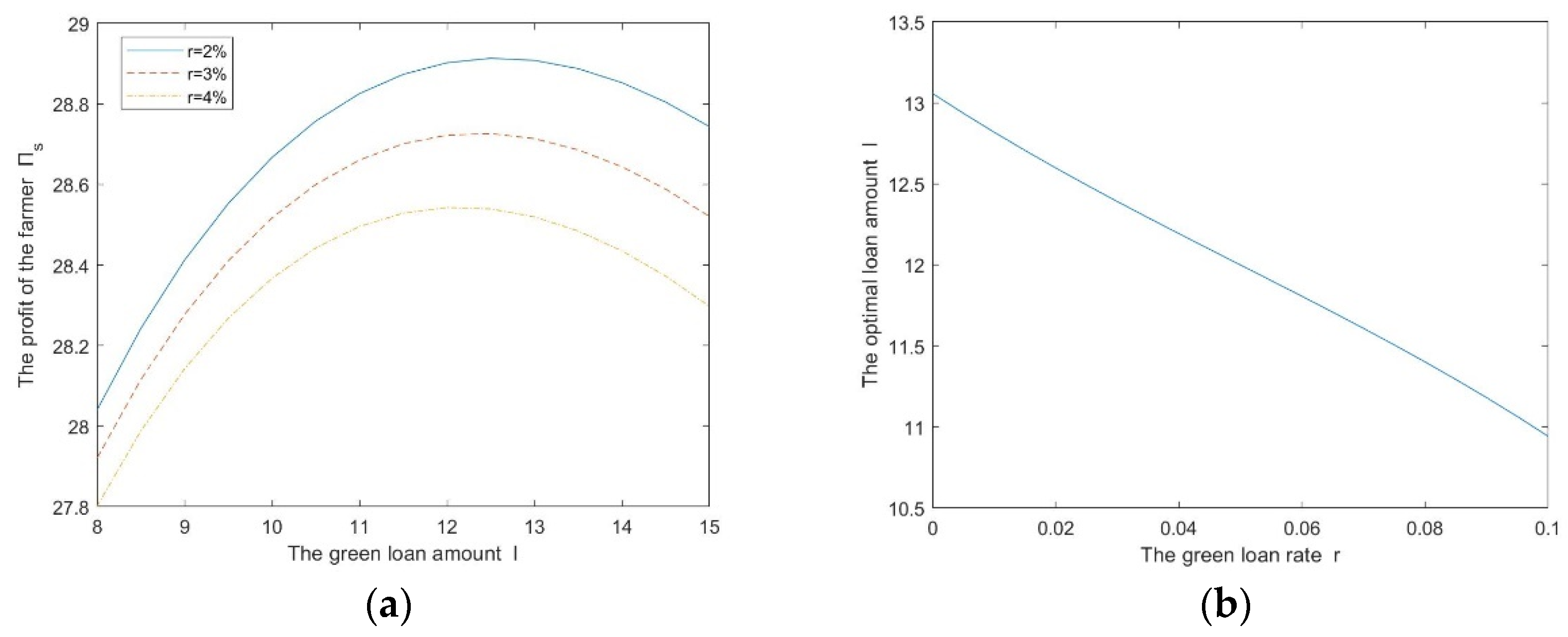
In the model we built, the farmer will decide his loan amount according to the interest rate set by the bank and then apply it in agricultural production. This means that for each green credit rate r given by the bank, the farmer should have a corresponding loan amount I that maximizes his expected profit under this loan rate and amount. Now, we investigate the sensitivity of the farmer’s profit to the green loan amount (Figure 2a). Moreover, based on the result, we also discuss the sensitivity of the farmer’s optimal loan amount to the green rate (Figure 2b).
We can calculate the expected profit of the farmer by giving the relevant parameters, as shown in Figure 2a, where the three curves from top to bottom indicate the variation of the farmer’s profit , with the loan amount I at a green credit rate r of 2%, 3% and 4%, respectively. It can be seen that the farmer’s expected profit rises and then falls as the loan amount increases. At the peak of the maximum profit of the farmer, we call the corresponding loan amount as the optimal loan amount. We can also find that the optimal loan amount becomes smaller as the loan interest rate increases. The relationship between optimal loan amount I and green loan interest rate r is given by Figure 2b. Figure 2b illustrates that as the loan interest rate increases, the loan amount applied by the farmer decreases. That is to say, a high interest rate will suppress the demand of loans.
After obtaining a loan, the farmer uses the loan for agricultural production and also has to make debt repayments according to the loan amount. Therefore, the amount of the loan not only affects the profit of the farmer’s output but also determines the pressure of the debt repayment. Agricultural production is risky, the production is highly affected by climate and natural disasters, leading to uncertainty in the output. For the farmer, the production is risky, and income is uncertain while the debt on the loan that the farmer needs to repay is certain. This means that the effect of raising the loan amount for the farmer is uncertain, and in the beginning, the increase in the loan amount will increase the input of production thus increasing the farmer’s revenue. When the loan amount increases to a certain extent, the gap between the uncertain income and the certain liabilities will become larger and larger, and the farmer’s income will gradually decrease as the loan amount increases. Therefore, the farmer will choose the best loan amount by measuring their income when facing each bank’s green loan interest rate.
4.2.2. Analysis of the Optimal Loan Rate and Profits
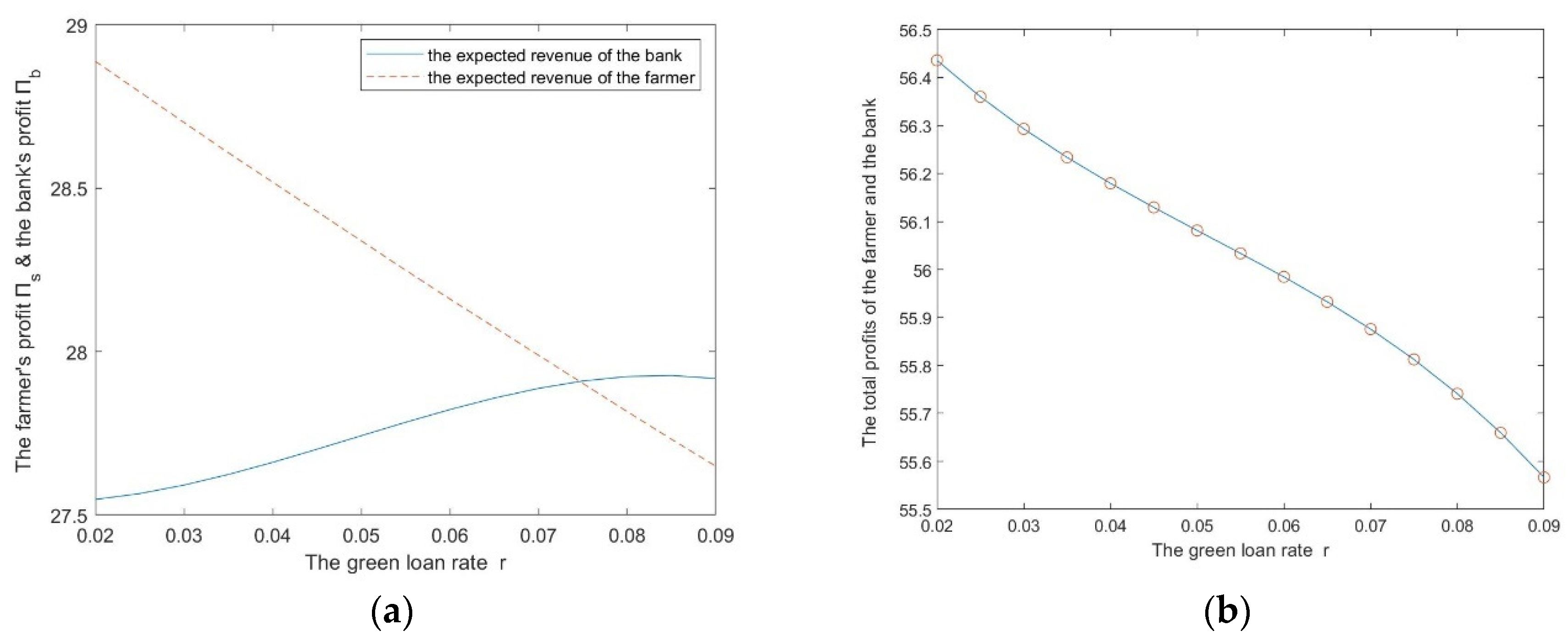
In the first subsection, we analyzed the optimal loan amount for the farmer. Now we will study the optimal loan rate for the bank and the profit of the bank and the famer. The results are shown in Figure 3a,b.
Figure 3a gives the profit of bank and farmer respectively at a interest subsidy rate F of 3%. Figure 3b shows how the total profits of the bank and the farmer change with changes of the interest rate at a interest subsidy rate F equals to 3%. In Figure 3a, the dotted line indicates the farmer’s profit . We can see that the farmer’s expected profit decreases with the increase of the green loan rate. It is because the increase in interest rates reduces the amount of the farmer’s loan, which in turn reduces his revenue. The solid line represents the bank’s profit . It can be seen that the bank’s expected profit first shows an upward trend as and then starts to decline after reaching a peak, so there is an optimal loan rate for the bank to maximize its profit. There are two effects of increasing the loan rate for the bank. First, the increase in interest rate will increase the bank’s interest income. Second, it will reduce the bank’s interest income by suppressing the amount of loans applied by the farmer. According to the simulated changes of the bank’s profit, it is easy to see that when the interest rate is at a low level, the former effect is greater than the latter one. However when the interest rate is at a high level, the latter effect is stronger than the former. Thus, the bank’s expected profit increases and then decreases with the increase of interest rate.
The comparison in Figure 3a shows that the farmers’ profit is more sensitive to interest rate changes, and the decrease in the farmer’s profit under the same interest rate fluctuations is greater than the increase in the bank’s profit, and vice versa. Therefore, as shown in the Figure 3b, the total profit of the farmer and the bank gradually decreases when the interest rate of the loan increases. Obtaining a loan for production is his only source of income for the farmer, but the bank is not. So, the risk resistance of the farmer is lower than it of the bank.
Generally, we can obtain some conclusions as follows. First, increasing the interest rate on green loans will inhibit the amount of loans applied by the farmer. Second, the expected profit of the farmer decreases with the increase of green loan interest rate, while the expected profit of the bank, on the contrary, increases with the increase of interest rate. Third, for the same scale of interest rate increase, the profit loss of the farmer is greater than the profit gain of banks. Finally, in the supply chain game framework, the bank can set the green loan rate that maximizes its own profit, and the farmer can choose their optimal loan amount to maximize their income level based on this rate. However, from the perspective of the whole supply chain, the optimum of each of them does not maximize the benefits of the supply chain as a whole.
4.3. Green Policy Sensitivity Analysis
From the previous section, it can be seen that the farmer chooses the best loan amount when the bank chooses the best loan rate of 8.5%. The overall benefits of the supply chain are not optimal at this time but it will be enhanced if the bank appropriately lower the loan rate. This subsection conducts a sensitivity analysis on the indicators of green policy to explore how the profits of the bank and the farmer change under the effect of green credit policy, and whether green credit policy can further enhance the benefits of the supply chain in the overall level.
4.3.1. Sensitivity Analysis of Interest Subsidy Rate
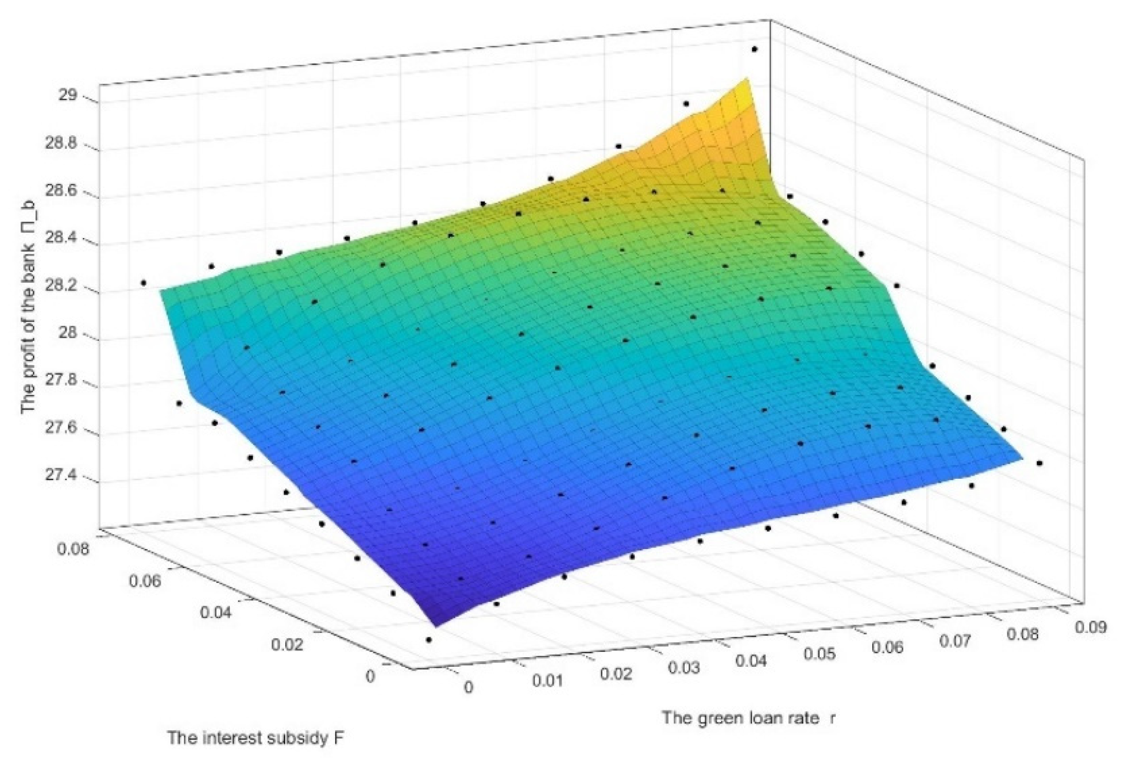
In the agricultural supply chain discussed in this paper, the commercial bank grant low-interest loans to the farmer, and the interest is subsidized by the finance department to the commercial bank. Then the subsidized interest is included in the bank’s profit calculation as part of the bank’s profit income. The subsidized interest rate is positively correlated with the amount of green loans lent by the bank, which in turn is influenced by the interest rate set by the bank itself. From the perspective of the interest subsidy rate, an increase in the subsidy rate will increase the amount of the subsidy and thus the bank’s income, and the bank will increase the interest subsidy income by lowering the interest rate to increase the loan amount if the incentive of the subsidy is large enough. But does this lead to a decrease in bank interest income of the loans? That is, does the increase in the discount rate have a dampening effect on the bank’s interest income? This is what will be discussed in this subsection (See Figure 4 and Figure 5).
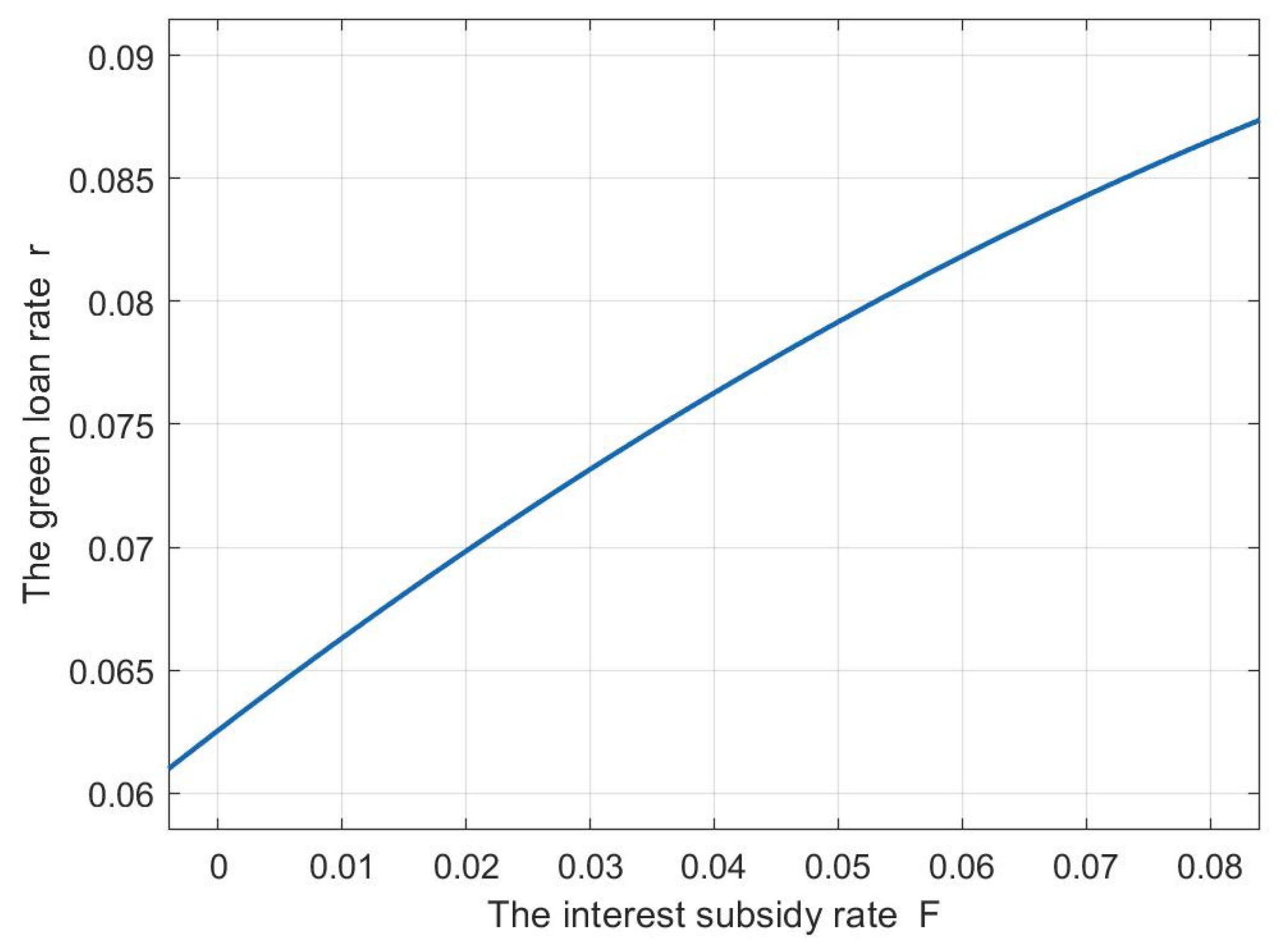
In Figure 4, the x-axis and the y-axis represent the green loan interest rate r set by the bank and the interest subsidy rate F, respectively. The z-axis represents the bank’s expected return . From Figure 4, it can be seen that the bank’s profit tends to increase with the increase in F. That is to say, the bank’s profit increases with the increase in the interest subsidy by the financial department. It shows that the green incentive policy of interest subsidy has a positive effect on the banks’ income. At the same time, we can note that the optimal green loan rate r is gradually increasing in the face of the gradually increasing subsidy rate F. We believe that the subsidy income caused by the increasing interest subsidy outweighs the interest rate loss that may result from an increase in the bank’s interest rate. Thus, it is profitable for banks to increase interest rate, and they choose to increase the interest rate on green loan in order to maximize their profits. The relationship between the interest subsidy rate F and the bank’s optimal loan rate r is shown in Figure 5, the optimal rate r will increase when the interest subsidy F increases.
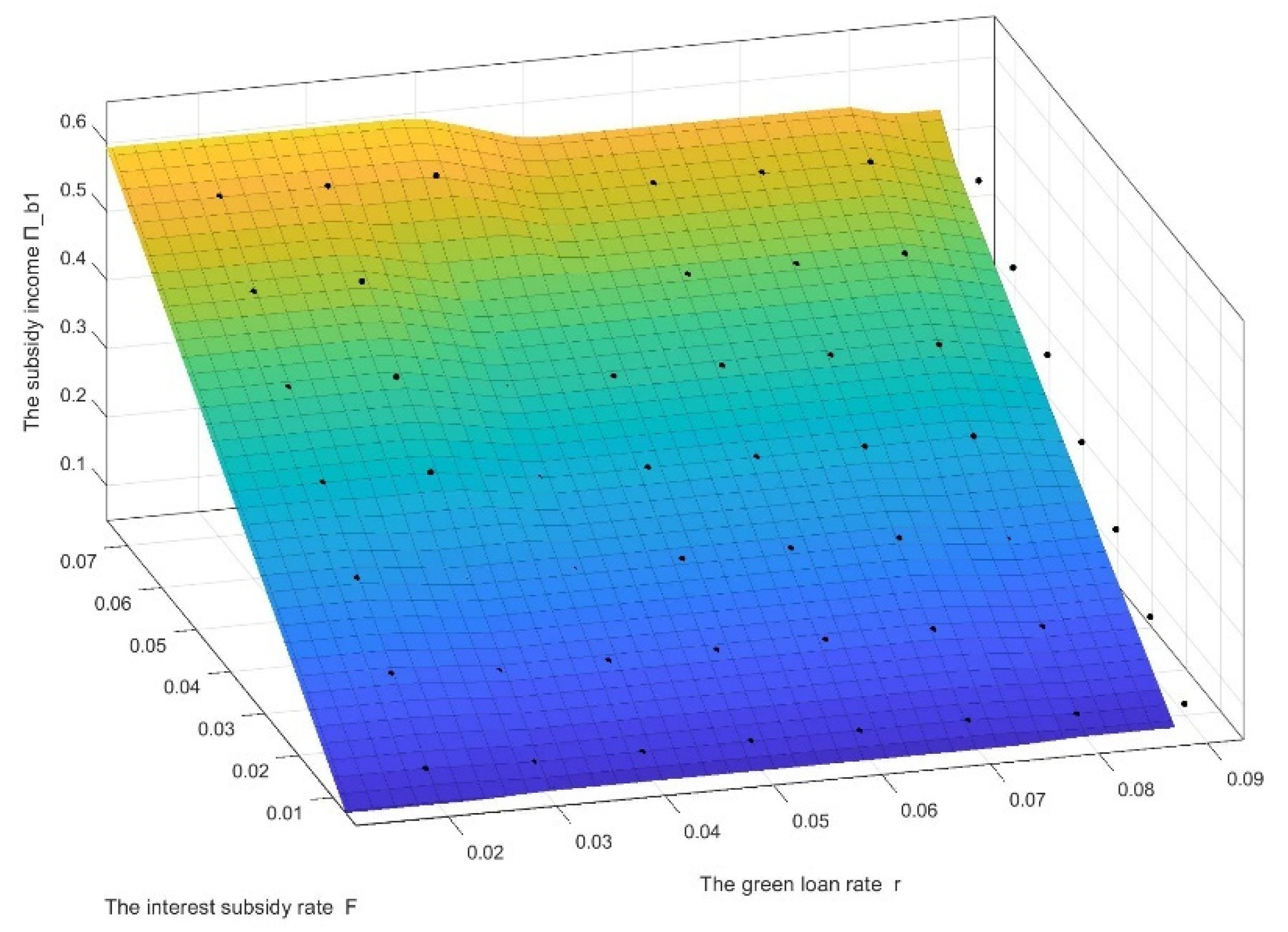
Next, we will study the impact of the interest rate and the subsidy rate on the bank’s subsidy income (Figure 6). Figure 6 shows how the bank’s subsidy income changes with the interest rate r and the subsidy rate F. From Figure 6, we can see that the subsidy income of the bank increases with the increase in the subsidy rate and the decrease in the loan rate. This is because a decrease in the interest rate brings an increase in the amount of the farmer’s loan, which brings an increase in the subsidy income. On the other hand, we can also see that as the green loan rate increases, the increase in subsidy income from an increase in the subsidy rate is reduced. This implies that a high interest rate diminishes the incentive effect of the interest subsidy rate policy on the bank.
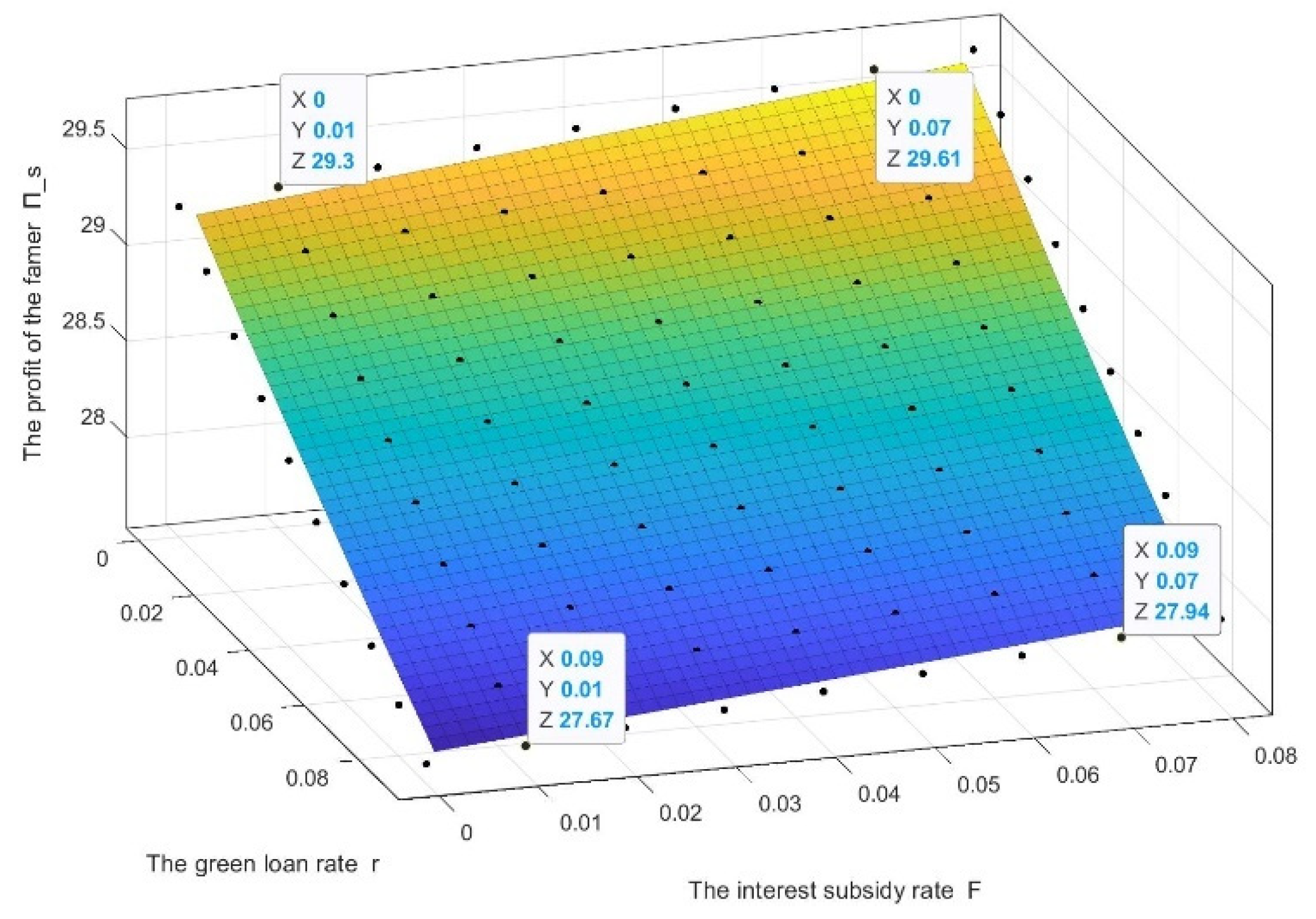
We further investigated how the interest subsidy rate affects the farmer’s expected profit (Figure 7). This had a similar reason for the effect in Figure 6 because the discounted income obtained by the bank is guided by the discount policy to give a portion of the discount to the farmer. The discount has an impact on the profit level of the farmer, as shown in Figure 7. As mentioned earlier, an increase in the interest rate leads to a decrease in the farmer’s expected profits. In contrast, an increase in the discount rate raises the income level of farmers. Additionally, we can observe that the decrease in farmer’s income due to the increase in interest rate decreases gradually when the subsidy rate is increasing gradually.
4.3.2. Sensitivity Analysis of Targeted Requirement Reserve Ratio Cuts
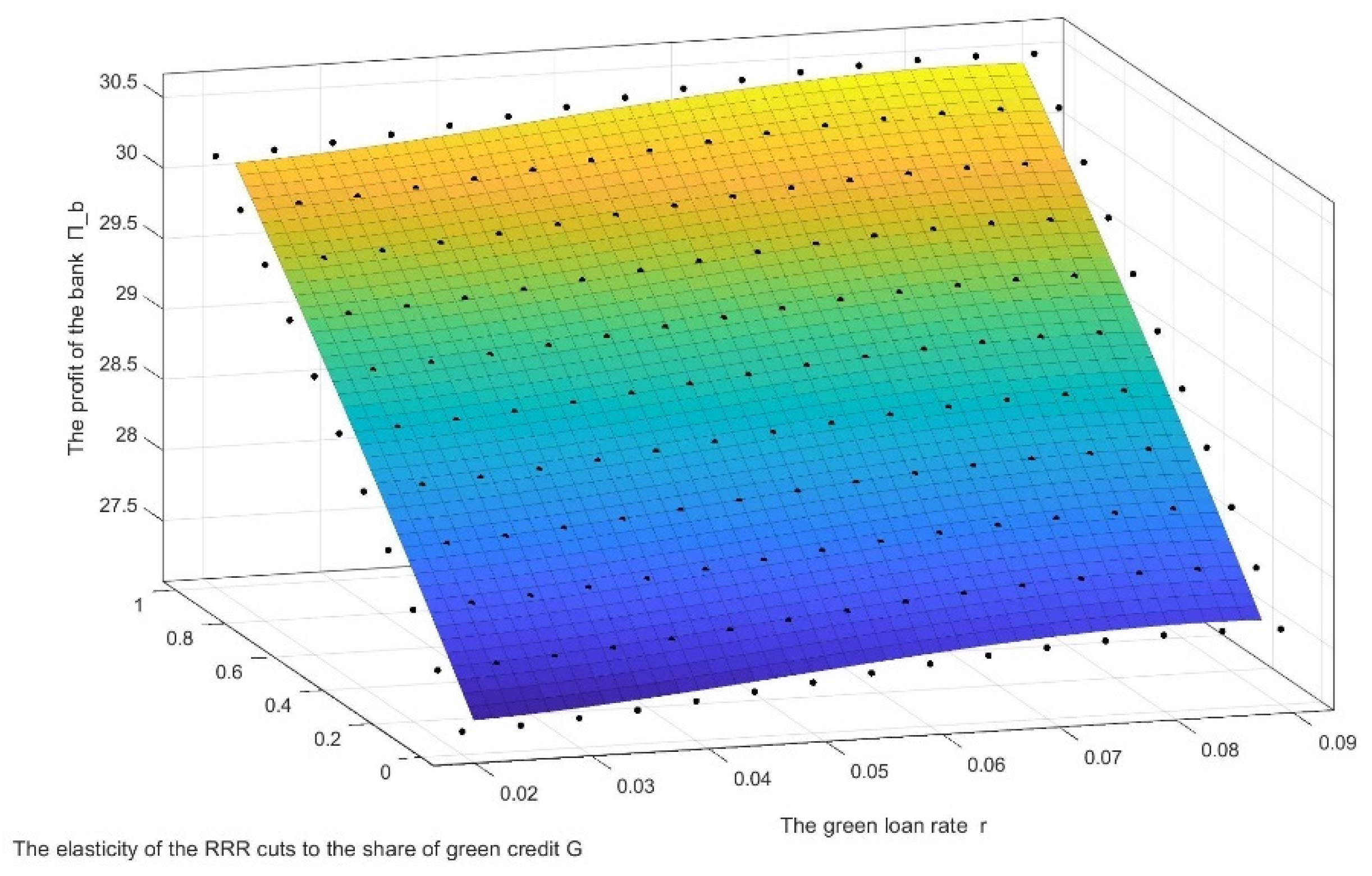
In addition to the interest subsidy policy given by the financial department, our model also considers a certain degree of targeted required reserve ratio (RRR) cuts given by the central bank to the commercial bank which issues green loans. In the discussion of this section, we will adjust the RRR cuts F indirectly by adjusting G, the elasticity of the RRR cuts to the share of green loan amount, and thus analyze the sensitivity of cuts to the RRR (Figure 8).
As shown in Figure 8, the overall profits of the bank increased with the increase in the elasticity indicator G. It indicates that the reduction policy of green credit is beneficial to enhance the efficiency of the whole supply chain. Likewise, the increase in bank’s profits brought by the increase in the green loan rate is gradually reduced in the process of increasing the RRR reduction rate. Conversely, the reduction in bank’s profits brought by the reduction in the green loan rate is also reduced. This indicates that under the effect of the RRR reduction policy, the bank that issued green loans have some room and incentive to lower the interest rate and give low-interest loans to the farmer, so as to further enhance the profitability of the supply chain.
5. Discussion
5.1. Research Results
In this paper, we build a Stackelberg model in which the bank sets the green loan rate as the leader, and the farmer chooses his own loan amount according to the bank’s rate as the follower. At the same time, the bank can predict the loan amount of the farmer and set the green loan rate based on it. Our study demonstrates that the optimal loan amount and the optimal loan interest rate exist in the green supply chain, and the increase in loan interest rate will suppress the loan amount of the farmer. In the game process, the bank and the farmer adopt their own optimal strategies, but they do not make the whole supply chain optimal, and there is large room for optimization. The implementation of green credit incentive policy has a positive effect on the utility of both the bank and the farmer. The green credit incentive policy gives income subsidies to farmers and banks, and expands the assets that banks can use for lending. In addition, the support from the finance department and the central bank to banks raises the income level of banks and reduces the degree of income loss due to the adjustment of interest rates by banks, giving them room to reduce the interest rate of loans, which helps to improve the overall utility level of the supply chain.
In previous studies of green supply chains, the income of each subject is calculated in terms of the success of the delivery of goods [50]. In contrast, this paper considers the characteristics of agricultural production and refers to relevant studies on agricultural supply chains to calculate the income of each subject in terms of the randomness of the production of agricultural products, which is more in line with the situation of agricultural production. For the discussion of green credit, previous studies have either investigated the connotation and model of green finance qualitatively [51], used general equilibrium models to study the effects of green credit policies [22] or used empirical methods to study the effects of corporate behavior on corporate governance under green finance policies [52]. This paper absorbs the discussion of green finance policy from previous studies and adopts the game model, which is widely used in supply chain research, in model construction, which is more suitable to develop the research on green supply chain finance.
5.2. Research Implications
The findings of this paper help to optimize the benefits of each subject in the agricultural supply chain, enhancing the overall efficiency of the agricultural supply chain. It has policy guidance significance for green finance-assisted agricultural development, which is conducive to achieving sustainable agricultural development. Based on the research results, we make the following policy recommendations.
Banks should combine agricultural production data and formulate different loan interest rate schemes for different agricultural products with different planting and breeding risks and market conditions. For agricultural products that are difficult to produce or scarce in the market, interest rates can be appropriately lowered to support farmers’ loan for agricultural production. On the other hand, for agricultural products with flood market supply or low crop value, the loan interest rate can be appropriately raised. Under the premise of risk control, the central bank and government departments can target the rate of green loan interest rate reduction, so that farmers and buyers can obtain greater returns, thus enhancing the overall benefits of the agricultural green supply chain. The central bank, commercial banks and local government departments should cooperate to expand the sources of funds needed for the implementation of green credit policies, such as green credit subsidies and green refinancing, and, furthermore, tax breaks for financial institutions, farmers and buyers need to be taken into account.
In addition, the application of green credit policies in the agricultural supply chain may come with some costs. First, in the presence of constraints on the total amount of loans, the increase in green credit may cause a decrease in other lending operations. For situations that the green-loan business crowd out other businesses, banks themselves should draw red lines for green loans. The central bank should expand banks’ green and non-green credit levels to cooperate with the implementation of green refinancing and RRR reduction policies. Second, the policy income may be larger than the normal output income with the increase in the loan amount, which may result in the excess of green production capacity and make the subjects supported by the policy obtain subsidies their main source of income. So, the finance department and the central bank should set a subsidy ceiling when implementing green credit policies to make sure that the production and sale of agricultural products are the main way for farmers to generate income. They should also adjust the flexibility of subsidies, considering the difficulty of agricultural production and market conditions, so that the green credit policies can really benefit farmers.
5.3. Outlook of the Further Problems
Future research can improve on our analyses as follows. First, the acquirer, an important subject in the supply chain, its purchase price and bargaining power will have a direct impact on the farmer’s revenue. However, we didn’t discuss the acquirer’s strategies. Second, the farmer’s financing approach discussed in this paper is single external financing, meaning that the loans are provided by the commercial bank. However, with the development of supply chain finance, internal financing within the industry has also been widely adopted. Therefore, the decision-making behavior of the three parties under such a financing model can be further examined when farmers adopt a dual-channel financing model, where loans are obtained from both the bank and the acquirer. Finally, the interest subsidy policy in this paper is a direct cash subsidy from the finance department to the farmer and the bank, which may put some pressure on the government finance department. Under the dual-channel financing mode, the tax of the acquirer can be reduced to some extent and the acquirer is required to provide low-interest loans to farmers, so as to reduce the financial pressure on the government.
6. Conclusions
Nowadays, countries around the world attach great importance to green and sustainable development. Green supply chain management is an effective way of sustainable development that gives consideration to both benefit and environment. At the same time, the Chinese government has put forward lots of policies for rural agricultural development in recent years. Agricultural green supply chain is the main direction for the sustainable development of agriculture in the future. Faced with the rapid development of agriculture and rural areas and the lack of relevant research, we conducted this study.
We used the Stackelberg Leadership Model to construct a pricing model which adds green credit policies. Our study on green credit shifted from the traditional macro level to the micro level. We introduced green credit to the traditional agricultural supply chain and investigated the impact of green credit policies on the green supply chain, and broadened the research content on agricultural supply chains. At the same time, considering that agricultural production is very affected by climate conditions, we formally applied randomness of agricultural output into our models. This makes the research method of supply chain finance more suitable for agriculture and closer to reality.
Through our study, we found that optimal decisions exist for both farmer and bank in the supply chain, but there is still room for optimization in the agricultural supply chain when both bank and farmer make their own optimal decisions. The implementation of green credit policies can improve the profit of subjects in agricultural supply chain. Green credit policies also give the bank room to reduce interest rates so that the overall utility level of the supply chain could be improved, which is conducive to efficiency and sustainable development. Therefore, the government should promote green credit policies in the agricultural supply chain to improve the overall efficiency of the supply chain, while giving benefits to the subjects in the supply chain.
Author Contributions
Conceptualization, L.D. and J.L.; methodology, L.D.; software, W.X.; validation, L.D., W.X. and J.L.; formal analysis, W.X.; investigation, J.L.; resources, L.D.; data curation, W.X.; writing—original draft preparation, L.D.; writing—review and editing, W.X.; visualization, J.L.; supervision, J.L.; project administration, L.D.; funding acquisition, L.D. All authors have read and agreed to the published version of the manuscript.
Funding
The article is supported by The National Social Science Fund of China (No. 19BGL002) and the Natural Science Foundation of Hunan Province ( NO.2018JJ3359).
Institutional Review Board Statement
Not applicable.
Informed Consent Statement
Not applicable.
Data Availability Statement
Not applicable.
Conflicts of Interest
The authors declare no conflict of interest.
Appendix A. Proof of Proposition 1
The farmer’s expected profit function is expressed as:
In this function, denotes the lower bound of the production efficiency in the natural production state and is the upper bound of the efficiency of the remaining production line in the natural production state, both of which are exogenous variables. The expression of is as follows:
Substitute (A2) into Equation (A1) and organize to obtain the Lagrange’s equation as follows:
The first-order derivative is:
Appendix B. Proof of Proposition 2
From the proof in Appendix A, it is clear that the loan amount can be solved by the rate when the Equation (A4) equals to 0. That is, is a function of , denoted as . The implicit expression of and is:
So, we can get the expression of as:
So,
It is clear that when , , and . That is, the optimal loan amount for the farmer decreases as the green loan interest rate set by the bank increases.
Appendix C. Proof of Proposition 3
The function of the bank’s expected profit is:
While the financial assets and liabilities identical equation of the bank is:
While there are equations as:
Based on the Equations of (A9)–(A12), we can get
Substituting (A13) into (A8), the Lagrange’s equation is obtained as:
The threshold , so the result of the first-order derivative of with respect to is:
So, the first-order derivative of the Lagrange’s equation is:
Substituting the expression of into the Equation (A16), and the following equation is obtained after collation:
We can get the following Equation (A18) by letting the formula (A17) equal zero:
Therefore, the optimal green loan interest rate set by the bank and the optimal loan amount for the farmer satisfy the following equation:
References
- Xu, Y.L.; Zhai, W.J. Financial friction and the function of rural financial subsidy policy in thedual economic transition process. J. Finan. Res. 2015, 2, 131–147. Available online: https://kns.cnki.net/kcms/detail/detail.aspx?FileName=JRYJ201502013&DbName=CJFQ2015 (accessed on 30 October 2021).
- Shen, Y.; Li, J.R.; Yang, J. Research on Poverty Reduction Mechanism Based on Financial Credit for Agricultural Supply Chain in the Background of Rural Revitalization--From the Perspective of Peasant Households’ Ability to Eliminate Poverty. J. Southwest Univ. 2019, 45, 50–60. Available online: https://kns.cnki.net/kcms/detail/detail.aspx?FileName=XBSW201902007&DbName=CJFQ2019 (accessed on 30 October 2021).
- Xie, P.; Xu, Z. Public Finance, Financial Support to Rural Area and Rural Finance Reform: Analysis of Survey in Guizhou Province and Sample Counties. Econ. Res. J. 2006, 4, 106–114. Available online: https://kns.cnki.net/kcms/detail/detail.aspx?FileName=JJYJ200604010&DbName=CJFQ2006 (accessed on 30 October 2021).
- Burgess, R.; Pande, R. Do rural banks matter? Evidence from the Indian social banking experiment. J. Am. Econ. Rev. 2005, 95, 780–795. [Google Scholar] [CrossRef] [Green Version]
- Lin, X.F. Current Situation and Prospects of Green Finance Supporting Green Building Development. Hous. Real. Estate 2020, 35, 67–70. Available online: https://kns.cnki.net/kcms/detail/detail.aspx?FileName=ZZFD202035022&DbName=CJFQ2020 (accessed on 30 October 2021).
- Chen, X.Z.; Yang, J.W.; Chen, R.Y.; Zhao, H.B.; Li, X.D.; Liu, D. Preliminary study on green finance supporting construction of happy rivers and lakes. J. Econ. Water Res. 2020, 38, 15–19. Available online: https://kns.cnki.net/kcms/detail/detail.aspx?FileName=SLJJ202006005&DbName=CJFQ2020 (accessed on 30 October 2021).
- Zhao, X.; Shan, X.W.; Ding, L.L.; Xue, Y.M. Application Analysis of Green Bonds in the Marine Economic Field. J. Mar. Econ. 2020, 10, 1–7. Available online: https://kns.cnki.net/kcms/detail/detail.aspx?FileName=SEJJ202006001&DbName=CJFQ2020 (accessed on 30 October 2021).
- Li, C.Y. An Overview of the application of green finance in the development of real economy. Fortune Today 2021, 2, 56–57. Available online: https://kns.cnki.net/kcms/detail/detail.aspx?FileName=JRCF202102025&DbName=CJFN2021 (accessed on 30 October 2021).
- Lee, J.W. Green finance and sustainable development goals: The case of China. J. Asian. Finan. Econ. Bus. 2020, 7, 577–586. [Google Scholar] [CrossRef]
- Li, S.; Jiang, H. Research on the Optimization and Upgrading of Industrial Structure Supported by Green Finance—Take Hebei Province as an example. Huabei Finan. 2021, 2, 87–94. Available online: https://kns.cnki.net/kcms/detail/detail.aspx?FileName=JRSC202102010&DbName=CJFQ2021 (accessed on 30 October 2021).
- Quan, H.; Gao, W.X. The Impact of Green Finance on the Eastern Economy Based on Demand Perspective. Sci. Technol. Ind. 2021, 21, 99–103. Available online: https://kns.cnki.net/kcms/detail/detail.aspx?FileName=CYYK202102015&DbName=CJFQ2021 (accessed on 30 October 2021).
- Wang, W.J.; He, T.Y.; Wu, H.M.; Shi, Y.T. Research on the Comprehensive Evaluation and Influencing Factors of Green Finance Development in Beijing-Tianjin-Hebei—Based on the Empirical Analysis of DEA-Tobit Model. Huabei Finan. 2021, 1, 28–41. [Google Scholar]
- Chen, T.Y.; Zuo, X.Y. Study on the Non-linear Economic Growth Effect of Green Financial Development. Foreign Econ. Relat. Trade 2020, 12, 101–104. Available online: https://kns.cnki.net/kcms/detail/detail.aspx?FileName=HLJW202012022&DbName=CJFQ2020 (accessed on 30 October 2021).
- Hu, M.D.; Zheng, H.R. Construction of Green Financial Risk Evaluation Index System and Governance Measures. Stat. Decis. 2020, 36, 129–132. Available online: https://kns.cnki.net/kcms/detail/detail.aspx?FileName=TJJC202024029&DbName=DKFX2020 (accessed on 30 October 2021).
- Zhang, G.Z.; Sun, H.M. Research on the Construction of Green Financial Performance Evaluation System. J. Reg. Financ. Res. 2020, 12, 5–11. Available online: https://kns.cnki.net/kcms/detail/detail.aspx?FileName=GXJR202012001&DbName=CJFQ2020 (accessed on 30 October 2021).
- Chen, H.B.; Zhao, X.L. Risk Management of Green Financial Investment Projects from the Perspective of Multi-party Game. Finan. Account. M. 2021, 1, 121–129. Available online: https://kns.cnki.net/kcms/detail/detail.aspx?FileName=CKYK202101018&DbName=CJFQ2021 (accessed on 30 October 2021).
- Gao, J.J.; Zhang, W.W. Research on the Impact of Green Finance on the Ecologization of China’s Industrial Structure—Empirical Test Based on System GMM Model. Econ. Rev. J. 2021, 2, 105–115. [Google Scholar]
- Bi, H.M.; Xiao, H.; Sun, K.J. The Impact of Carbon Market and Carbon Tax on Green Growth Pathway in China: A Dynamic CGE Model Approach. Emerg. Mark Financ. Tr. 2019, 55, 1312–1325. [Google Scholar] [CrossRef]
- Hector, P.; Francois, J.M. The role of money and the financial sector in energy-economy models used for assessing climate and energy policy. Clim. Policy 2018, 18, 184–197. [Google Scholar] [CrossRef] [Green Version]
- Song, X. Empirical Study on the General Equilibrium of Green Credit Transmission Path in China. Financ. Regul. Res. 2016, 5, 87–97. Available online: https://kns.cnki.net/kcms/detail/detail.aspx?FileName=JRJG201605006&DbName=CJFQ2016 (accessed on 30 October 2021).
- Liu, J.Y.; Xia, Y.; Lin, S.M.; Wu, J.; Fan, Y. The Short, Medium and Long Tern Effects of Green Credit Policy in China Based on a Financial CGE Model. Chin. J. Manag. Sci. 2015, 23, 46–52. Available online: https://kns.cnki.net/kcms/detail/detail.aspx?FileName=ZGGK201504006&DbName=CJFQ2015 (accessed on 30 October 2021).
- Liu, J.Y.; Xia, Y.; Fan, Y. Assessment of a green credit policy aimed at energy-intensive industries in China based on a financial CGE model. Clean Prod. 2017, 163, 293–302. [Google Scholar] [CrossRef]
- Wang, Z.Y.; Xiong, Z. The Study on Influence Period of the Green Credit Policy Based on CGE Model. In Proceedings of the 2017 4th International Conference on Education, Management and Computing Technology (ICEMCT 2017); Atlantis Press:: Paris, France, 2017. Available online: www.atlantis-press.com (accessed on 30 October 2021).
- Barbara, A.; Dio, D. GHG Emissions Control and Monetary Policy. Environ. Resour. Econ. 2017, 67, 823–851. [Google Scholar] [CrossRef] [Green Version]
- Wang, Y.; Pan, D.Y.; Peng, Y.C.; Liang, X. China’s Incentive Policies for Green Loans: A DSGE Approach. J. Financ. Res. 2019, 11, 1–18. Available online: https://kns.cnki.net/kcms/detail/detail.aspx?FileName=JRYJ201911001&DbName=CJFQ2019 (accessed on 30 October 2021). [CrossRef]
- Preuss, L. In dirty chains? Purchasing and greener manufacturing. J. Bus. Ethics. 2001, 34, 345–359. [Google Scholar] [CrossRef]
- Srivastava, S.K. Green supply-chain management: A state-of-the-art literature review. Intern. J. Manag. Rev. 2007, 9, 53–80. [Google Scholar] [CrossRef]
- Fatemi, A.M.; Fooladi, I.J. Sustainable finance: A new paradigm. Glob. Finan. J. 2013, 24, 101–113. [Google Scholar] [CrossRef]
- Forcella, D.; Hudon, M. Green microfinance in Europe. J. Bus. Ethics 2016, 135, 445–459. [Google Scholar] [CrossRef]
- Yang, H.X.; Duan, W.Y. Research on Financing Mode for Capital Constrained Manufacturer in Green Supply Chain. Oper. Res. Manag. Sci. 2019, 28, 126–133. [Google Scholar] [CrossRef]
- Deng, L.; Yang, L.; Li, W. Impact of Green Credit Financing and Carbon Emission Limits on the Supply Chain Based on POF. Sustainability-Basel 2021, 13, 5814. [Google Scholar] [CrossRef]
- Li, B.; Zhu, M.; Jiang, Y.; Li, Z. Pricing policies of a competitive dual-channel green supply chain. Clean. Prod. 2016, 112, 2029–2042. [Google Scholar] [CrossRef]
- Johari, M.; Hosseini-Motlagh, S.M.; Rasti-Barzoki, M. An evolutionary game theoretic model for analyzing pricing strategy and socially concerned behavior of manufacturers. Transp. Res. Part E 2019, 128, 506–525. [Google Scholar] [CrossRef]
- Zhao, J.; Tang, W.; Zhao, R.; Wei, J. Pricing decisions for substitutable products with a common retailer in fuzzy environments. Eur. J. Oper. Res. 2012, 216, 409–419. [Google Scholar] [CrossRef]
- Wang, L.; Song, Q. Pricing policies for dual-channel supply chain with green investment and sales effort under uncertain demand. Math. Comput. Simulat. 2020, 171, 79–93. [Google Scholar] [CrossRef]
- Zhang, C.T.; Wang, H.X.; Ren, M.L. Research on pricing and coordination strategy of green supply chain under hybrid production mode. Comput. Ind. Eng. 2014, 72, 24–31. [Google Scholar] [CrossRef]
- Sun, Y.; Wang, Y.; Li, T. The designation of agriculture supply chain management. In Proceedings of the DSS 2007 IEEE International Conference on Automation and Logistics, Jinan, China, 18–21 August 2007; IEEE: Manhattan, NY, USA, 2007; pp. 1492–1497. [Google Scholar] [CrossRef]
- Lin, Q.; Ye, F. Coordination For ‘Company + Farmer’ Contract-Farming Supply Chain Under Nash Negotiation Model. Syst. Eng. Theory Pract. 2014, 34, 1769–1778. Available online: https://kns.cnki.net/kcms/detail/detail.aspx?FileName=XTLL201407014&DbName=CJFQ2014 (accessed on 30 October 2021).
- Peng, H.J.; Pang, T. Financing and operational strategies for the contract-farming supply chain under agricultural subsidy policy. J. Ind. Eng. Manag. 2020, 34, 155–163. Available online: https://kns.cnki.net/kcms/detail/detail.aspx?FileName=GLGU202005017&DbName=CJFQ2020 (accessed on 30 October 2021).
- Hirbod, A.; Hossein, S.; Andrew, L. An examination of the role of price insurance products in stimulating investment in agriculture supply chains for sustained productivity. Eur. J. Oper. Res. 2021, 288, 703–1084. [Google Scholar] [CrossRef]
- Yang, Z.R.; Dong, Q.Y. Research on Risk Generation Mechanism and Prevention of Agricultural Supply Chain Finance from Internet Perspective. Light. Ind. Sci. Technol. 2020, 36, 115–116. Available online: https://kns.cnki.net/kcms/detail/detail.aspx?FileName=GXQG202012050&DbName=CJFQ2020 (accessed on 30 October 2021).
- Zhang, D.B. Research on Risk Sources and Risk Control of Agricultural Supply Chain Finance. Agr. Econ. 2017, 6, 95–96. [Google Scholar]
- De, A.; Singh, S.P. Analysis of Fuzzy Applications in the Agri-Supply Chain: A Literature Review. J. Clean. Prod. 2020, 283, 124577. [Google Scholar] [CrossRef]
- Hu, S.S.; Huang, S.; Huang, J.; Su, J.F. Blockchain and Edge Computing Technology Enabling Organic Agricultural Supply Chain: A Framework Solution to Trust Crisis. Comput. Ind. Eng. 2021, 153, 107079. [Google Scholar] [CrossRef]
- Wang, K.Y.; Yan, X.X.; Fu, K.Y. Research on Risk Management of Agricultural Products Supply Chain Based on Blockchain Technology. Open. J. Bus. Manag. 2020, 8, 2493–2503. [Google Scholar] [CrossRef]
- Zhu, X.K.; Han, L.; Zeng, C.C. The Relationship between the Information and the Fluctuation of Agricultural Products: An Analysis Based on the EGARCH Model. Manag. World 2012, 11, 57–66. Available online: https://kns.cnki.net/kcms/detail/detail.aspx?FileName=GLSJ201211006&DbName=CJFQ2012 (accessed on 30 October 2021).
- Cai, X.; Chen, J.; Xiao, Y. Optimization and Coordination of Fresh Product Supply Chains with Freshness-Keeping Effort. Prod. Oper. Manag. 2010, 19, 261–278. [Google Scholar] [CrossRef]
- Ye, F.; Lin, Q.; Mo, R.J. Contract-farming supply chain coordination mechanism based on B-S model. J. Manag. Sci. Chin. 2012, 15, 66–76. [Google Scholar]
- Chen, Y.H.; Tu, H.Y.; Zeng, Y. Loan pricing and production adjustment mechanism in agricultural supply chain finance. Syst Eng. Theory Practice 2018, 38, 1706–1716. [Google Scholar]
- Tang, C.S.; Yang, S.A.; Wu, J. Sourcing from suppliers with financial constraints and performance risk. M&SOM-Manuf. Serv. Op. 2018, 20, 70–84. [Google Scholar] [CrossRef] [Green Version]
- An, W. A Probe into the Connotation, Mechanism and Practice of Green Finance. Econ. Surv. 2008, 5, 156–158. Available online: https://kns.cnki.net/kcms/detail/detail.aspx?FileName=JJJW200805049&DbName=CJFQ2008 (accessed on 30 October 2021).
- Yang, Y.; Li, Y.X.L.; Shen, H.T. Green Financial Policies, Corporate Governance and Environmrntal Disclosure: A Case Study of 502 Listed Firms in Heavy Pollution Industry. Finan. Trade Res. 2011, 22, 131–139. Available online: https://kns.cnki.net/kcms/detail/detail.aspx?FileName=CMYJ201105020&DbName=CJFQ2011 (accessed on 30 October 2021).
Figure 1.
Flow chart of agricultural supply chain finance based on green credit.

Figure 2.
The profit realized (a) by and optimal loan amount (b) for the farmer.

Figure 3.
The expected profit of the bank and the farmer individually (a) and in total (b).

Figure 4.
The impact of the interest subsidy rate on the banks’ expected profit.

Figure 5.
The impact of the interest subsidy rate on the bank’s optimal rate.

Figure 6.
The impact of r and F on the bank’s subsidy income.

Figure 7.
The impact of the interest subsidy rate on the farmer’s expected profit.

Figure 8.
The impact of RRR cuts on the bank’s expected profits.


Table 1.
Definition of Parameters.
| Symbol | Parameter Name | Definition | Value |
|---|---|---|---|
| Production efficiency | Represents the unit output brought by unit capital | ||
| m | The buyer’s bargaining power | The buyer can buy the product with a price discount of m | 0.75 |
| k | Inverse of the price elasticity of demand | The demand responsiveness to product price | 1/1.8 |
| Choke price | The market price of agricultural products when production is 1 unit | 15 | |
| s | Required Reserve Ratio | The minimum required proportion of reserves that banks are required by the central bank to keep on hand and not loan out. | 15% |
| Green refinance rate | Rate the bank lends from the central bank | 5% | |
| Non-green loan rate | Interest rates for non-green loan business | 6% | |
| Deposit Rate | The interest rate at which the bank repay household deposits | 3% | |
| H | Green refinance | Number of refinancing loans obtained by banks from the central bank | -- |
| M | Pledge Rate | H = M × I | 0.5 |
| F | Interest subsidy rate | The rate of interest subsidy, and the total amount of the subsidy is F × I | 0.03 |
| V | Required reserve ratio cuts | The reduction on required reserve ratio | -- |
| G | Elasticity of the RRR cuts to the share of green credit | The RRR cuts responsiveness to the share of green credit | 0.1 |
| q | Bank’s share of interest subsidy | Percentage of interest subsidy received by the bank | 0.6 |
The currency unit is CNY (¥).
Publisher’s Note: MDPI stays neutral with regard to jurisdictional claims in published maps and institutional affiliations. |
© 2021 by the authors. Licensee MDPI, Basel, Switzerland. This article is an open access article distributed under the terms and conditions of the Creative Commons Attribution (CC BY) license (https://creativecommons.org/licenses/by/4.0/).
Share and Cite
MDPI and ACS Style
Deng, L.; Xu, W.; Luo, J. Optimal Loan Pricing for Agricultural Supply Chains from a Green Credit Perspective. Sustainability 2021, 13, 12365. https://0-doi-org.brum.beds.ac.uk/10.3390/su132212365
AMA Style
Deng L, Xu W, Luo J. Optimal Loan Pricing for Agricultural Supply Chains from a Green Credit Perspective. Sustainability. 2021; 13(22):12365. https://0-doi-org.brum.beds.ac.uk/10.3390/su132212365
Chicago/Turabian StyleDeng, Liurui, Wentang Xu, and Juan Luo. 2021. "Optimal Loan Pricing for Agricultural Supply Chains from a Green Credit Perspective" Sustainability 13, no. 22: 12365. https://0-doi-org.brum.beds.ac.uk/10.3390/su132212365
Note that from the first issue of 2016, this journal uses article numbers instead of page numbers. See further details here.