Tropical Forests Classification Based on Weighted Separation Index from Multi-Temporal Sentinel-2 Images in Hainan Island

Abstract

Tropical forests play a vital role in biodiversity conservation and the maintenance of sustainability. Although different time-series spatial resolution satellite images have provided opportunities for tropical forests classification, the complexity and diversity of vegetation types still pose challenges, especially for distinguishing different vegetation types. In this paper, we proposed a Spectro-Temporal Feature Selection (STFS) method based on the Weighted Separation Index (WSI) using multi-temporal Sentinel-2 data for mapping tropical forests in Jianfengling area, Hainan Province. The results showed that the tropical forests were classified with an overall accuracy of 93% and an F1 measure of 0.92 with multi-temporal Sentinel-2 data. As our results also revealed, the WSI based STFS method could be efficient in tropical forests classification by using a fewer feature subset compared with Variable Selection Using Random Forest (14 features and all 40 features, respectively) to achieve the same accuracy. The analysis also showed it was not advisable to only pursue a higher WSI value while ignoring the heterogeneity and diversity of features. This study demonstrated that the WSI can provide a new feature selection method for multi-temporal remote sensing image classification.

1. Introduction

Tropical forests play an important role in biodiversity protection, regulation of climate change, prevention of soil erosion, and carbon sink estimation [1,2]. It is one of the foundations of natural resources and the ecological environment. Tropical forests produce and store 40% of the world’s biomass carbon, which is extremely important for the global carbon cycle and ecological security closely related to humans. Tropical forests are the largest terrestrial component of the global carbon budget [3,4], which accounts for 50% of the carbon stored in the global vegetation (350–600 Gt C) [5,6].

The idea of sustainability has become a watchword in recent years, and the definitions of sustainability are important for tropical forest managers, policymakers, and governments. The connection between the tropical forest and sustainability is complex [7]. Since UNCED in 1992, several international processes and initiatives have developed criteria and indicators as frameworks for sustainable forest management. The Food and Agriculture Organization (FAO) of the United Nations defined sustainable forest management as the “application of forest management practices for the primary purpose of sustaining constant levels of carbon stocks over time” [8]. However, due to human overutilization, the annual rate of tropical forest deforestation has increased year by year [9,10]. Since 1990, about 420 million hectares of tropical forests have been converted to other uses. Therefore, conducting tropical forest surveys and obtaining timely and accurate information on vegetation types and coverage is the focus of this study [9].

Earth Observation (EO) techniques have proved to be a very effective and cost-efficient approach for forest mapping compared to traditional field surveys [11]. Most tropical forest monitoring systems use optical data sets and focus on large deforestation areas, with user accuracies of 90% and producer accuracies of 75% [12]. Recent developments have led to automated forest classifications that are based on the coarse resolution MODIS (Moderate Resolution Imaging Spectroradiometer) sensor and allow tracking forest changes in near real-time (NRT), such as Global Forest Watch Alerts [13]. Most studies have therefore turned to Landsat data, which have higher resolution (30 m) [14,15], or a combination of MODIS and Landsat.

With the launch of the European Space Agency’s Copernicus Sentinel-2A/B satellites recently, medium–high resolution data have become more available. Compared to Landsat imagery (7/8 bands, 30 m 8/16 days), which is commonly used in forests classification [16], Sentinel-2 has a clear improvement in spatial and temporal resolution [17]. Although more abundant data sources have brought opportunities for tropical forests classification, new challenges have emerged [18]. The number of features which are used as input to the classification has exponentially increased.

The use of datasets with a very large number of predictors may relate to (i) overfitting the classification algorithm due to random variation from irrelevant features captured as meaningful information, (ii) constructing intrinsically complex models which might make model interpretation a challenging task, and, finally, (iii) requiring additional computational effort, data storage, and processing than a simpler, more parsimonious dataset would [19].

To tackle these issues, feature selection (FS) may be applied, where the classification model is fit on a reduced subset of the most discriminant and informative predictors. The methods select cost-effective predictors form a large number of variables, improve performance of predictors, and provide insights into the underlying interactions of data [20]. In environmental applications, feature selection methods based on simple statistical tests (e.g., Pearson’ correlation coefficient and Wilks criterion) or wrapped in certain algorithms (e.g., Variable selection based on Random Forest) have been applied in classification [18]. They were used to reduce data complexity by extracting relevant information from multi-spectral satellite imagery [21,22], and to find relatively significant features in order to improve prediction accuracy for specific land cover types [23]. Somers and Asner [24] proposed the separability index (SI), which used the ratio of the spectral difference inter- and intra-classed, and achieved a better classification result in distinguishing different land use types.

However, the Separability Index (SI) can only indicate the degree of separation between two types of features, and can not effectively distinguish three or more types. The performance of variable selection varies with different criteria used. There is no consensus made on the preference of a feature selection method for tropical forests classification with remotely sensing data. Therefore, in this paper, we proposed the Weighted Separation Index (WSI) to overcome the problem that SI can not effectively distinguish more than two types. Then the Spectro-Temporal Feature Selection (STFS) method using multi-temporal Sentinel-2 data based on WSI was implemented in Jianfengling area, Hainan Province, to verify the effect of the the WSI.

2. Study Area and Data

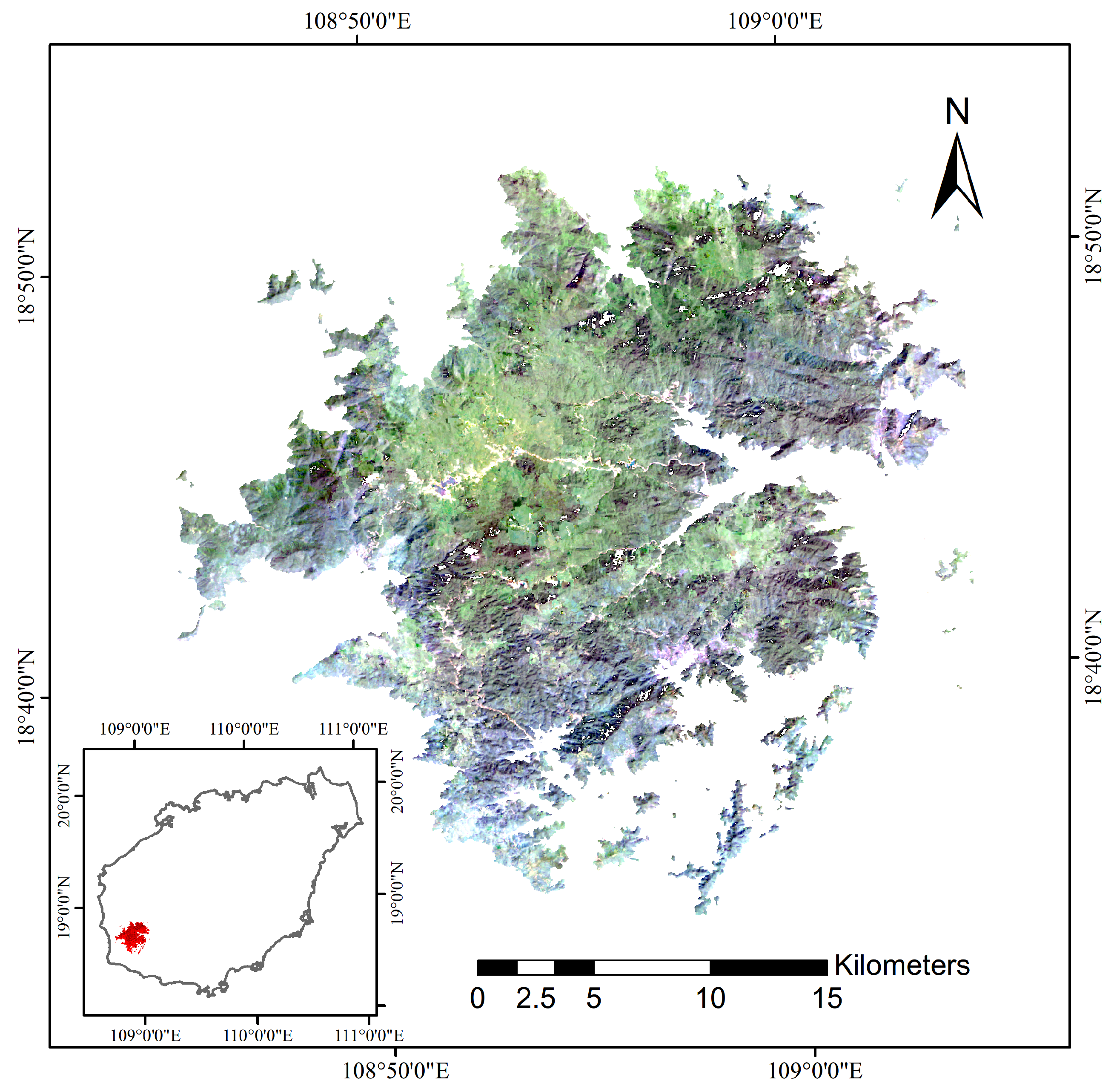
2.1. Jianfengling Research Area, Hainan Island

Hainan Island (Shown in the lower left corner of Figure 1) is located south of the Leizhou Peninsula of China, and is surrounded by the Qiongzhou Strait, the Beibu Gulf, and the South China Sea. It is the second largest island of China, with an area of 34,000 km ${}^2$. The island is located in the tropical climate region, and the specific location is 3.30° N∼20.07° N, 108.15° E∼120.05° E. The elevation in this island ranges from circa 100 m to 1800 m above sea level, and the terrain varies from plains to mountains. Annual precipitation ranges between 900 and 2600 mm, decreasing from east to west. The average annual temperature is about 25 °C, and the climate includes a rainy season and a dry season. Due to its climatic conditions and fertile soil, Hainan Island has abundant vegetation and high forest coverage. It still retains the most preserved and pristine tropical forests in China.

Jianfengling area, located at the junction of Ledong Li Autonomous County and Dongfang City, lies in the southwest of Hainan Province, with a total area of 640 km ${}^2$ (Figure 1). The Jianfengling area has a low-latitude tropical island monsoon climate. The annual rainfall is unevenly distributed, with obvious dry and wet seasons.The average annual temperature in the dry season reaches 27 °C∼29 °C, while air temperature in the wet season reaches 16.2 °C∼20.6 °C [25]. The natural environment in this area is superior and suitable for vegetation growth, which provides conditions for the existence of a large and intact tropical virgin forest in China. The forest coverage rate is 93.18%, including mountain tops, moss dwarf forest, tropical mountain evergreen broad-leaved forest, tropical mountain rainforest, tropical evergreen monsoon forest, tropical semi-deciduous monsoon forest, and other typical tropical vegetation types. It is an ideal area for conducting remote sensing classification research on tropical forests.

2.2. Data

In this study, Sentinel imagery was sourced, accessed, and processed based on Google Earth Engine (GEE), a cloud-based platform for analyzing planetary-scale environment data. In addition, auxiliary data (e.g., elevation) were also used.

2.2.1. Sentinel-2 Data

The Sentinel-2 mission consists of two satellites, Sentinel-2A and Sentinel-2B. Both satellites carry MSI (Multispectral imager) sensors, including 13 multispectral bands which span from the visible (VIS) and the near infrared (NIR) to the short wave infrared (SWIR) at different spatial resolutions at the ground ranging from 10 to 60 m (

Table 1. The central wavelength and spatial resolution for Sentinel-2 bands used in this study.

Bands	Wave-Length (nm)	Resolution (m)
Band2—Blue	490	10
Band3—Green	560	10
Band4—Red	665	10
Band5—Red edge 1	705	20
Band6—Red edge 2	740	20
Band7—Red edge 3	783	20
Band8—NIR	842	10
Band11—SWIR	1610	20
Band12—SWIR	2190	20

). Frequent revisits of five days at the equator require two identical Sentinel-2 satellites operating simultaneously favoring a small, cost-effective, and low-risk satellite [26]. For each satellite, the replay period is 10 days, and a constellation composed of two satellites can reach a revisit period of 5 days.

In the GEE data catalog, Sentinel-2 MSI data contain two products, Level-1C and Level-2A. The Level-1C product has been orthorectified and geographically registered, and the Level-2A product has been atmospherically corrected based on Level-1C product [27]. However, the Level-2A product before 2019 cannot be downloaded from GEE, therefore, we used the Sentinel-2 imagery (Level 1C Top-of Atmosphere reflectance products) in 2018 with 10 m and 20 m resolutions. The reason why we did not adopt the rest of the bands in Sentinel-2 imagery is that the spatial resolution of these bands is 60 m, which is too rough for tropical forest classification. Finally, we collected 69 images from the GEE platform covering the Jianfengling area.

2.2.2. Auxiliary Data

• Land Use Classification Map of Hainan Province. This paper obtains the remote sensing monitoring data of China’s land use in Hainan Province in 2018 through the website of the Institute of Geographical Sciences and the Institute of Natural Resources Research, Chinese Academy of Sciences, with a resolution of 1 km ${}^2$. The land use types in Hainan Province mainly include 6 first-level types and 25 s-level types of cultivated land, forest land, water area, and residential land. In this paper, the obtained classification file is imported into GEE and filtered by codes to obtain the distribution map of the main forest land in Hainan, which makes it easier to acquire the experimental area boundary.
• Digital Elevation Model (DEM) data in Hainan. In order to facilitate subsequent sample selection and result verification, this paper obtained SRTM (The Shuttle Radar Topography Mission) elevation data from the GEE database. Our observation showed that the Jianfengling forest area has an obvious elevation from the coastal area (average altitude of 50 m) to the forest hinterland, and the elevation of the eastern area is significantly higher than that of the west.

2.2.3. Fieldwork Data

According to the Hainan Forest vegetation classification system proposed by Song Yongchang [28] and referring to the field survey results in the Jianfengling Experimental Area, this paper divided the tropical forests in this area into typical tropical rainforests, tropical monsoon forests, and evergreen broad-leaved forest. The classification level belongs to the third level of vegetation type.

The field survey data used in this paper were obtained in Hainan Island in 2016. More than 400 forest-type plots were recorded in the survey, and 580 samples in total were collected from the filed survey [29]. According to the survey, the main types of natural forests in the Jianfengling area of Hainan Island include tropical forests, typical tropical rainforests, tropical monsoon forests, and evergreen broad-leaved forests. Figure 2 shows the field photos of different types of tropical forests obtained during the investigation. According to the investigation, the specific characteristics of Hainan’s tropical forest types are as follows:

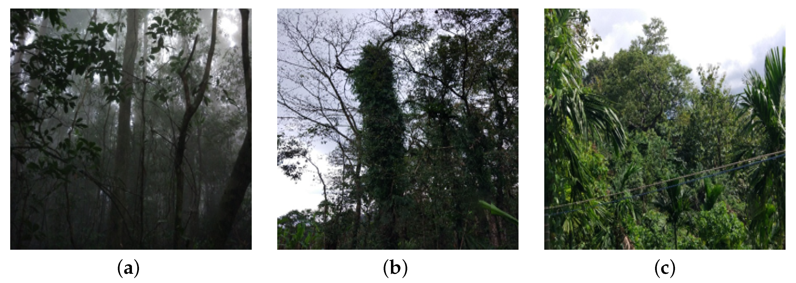
• Typical tropical rainforest: Vegetation is flourishing, with rich tree species diversity and basically no human influence. The spatial structure is obvious, generally stratified into 5–7 layers, including herb, shrub, young tree, general tree, and tall arbor layers.
• Evergreen broad-leaved forest: It has serious human impact and non-defined stratification, with generally only 1–2 layers, i.e., a shrub and an arbor layer. The deciduous tree species are eucalyptus, maple, Hainan bean, and others.
• Tropical monsoon forest: It is affected by humans to a certain extent. Its stratification has 3–4 layers. The forest presents some seasonality, such as deciduous leaf and the color change of leaves. The main tree species are rose apple and eucalyptus.

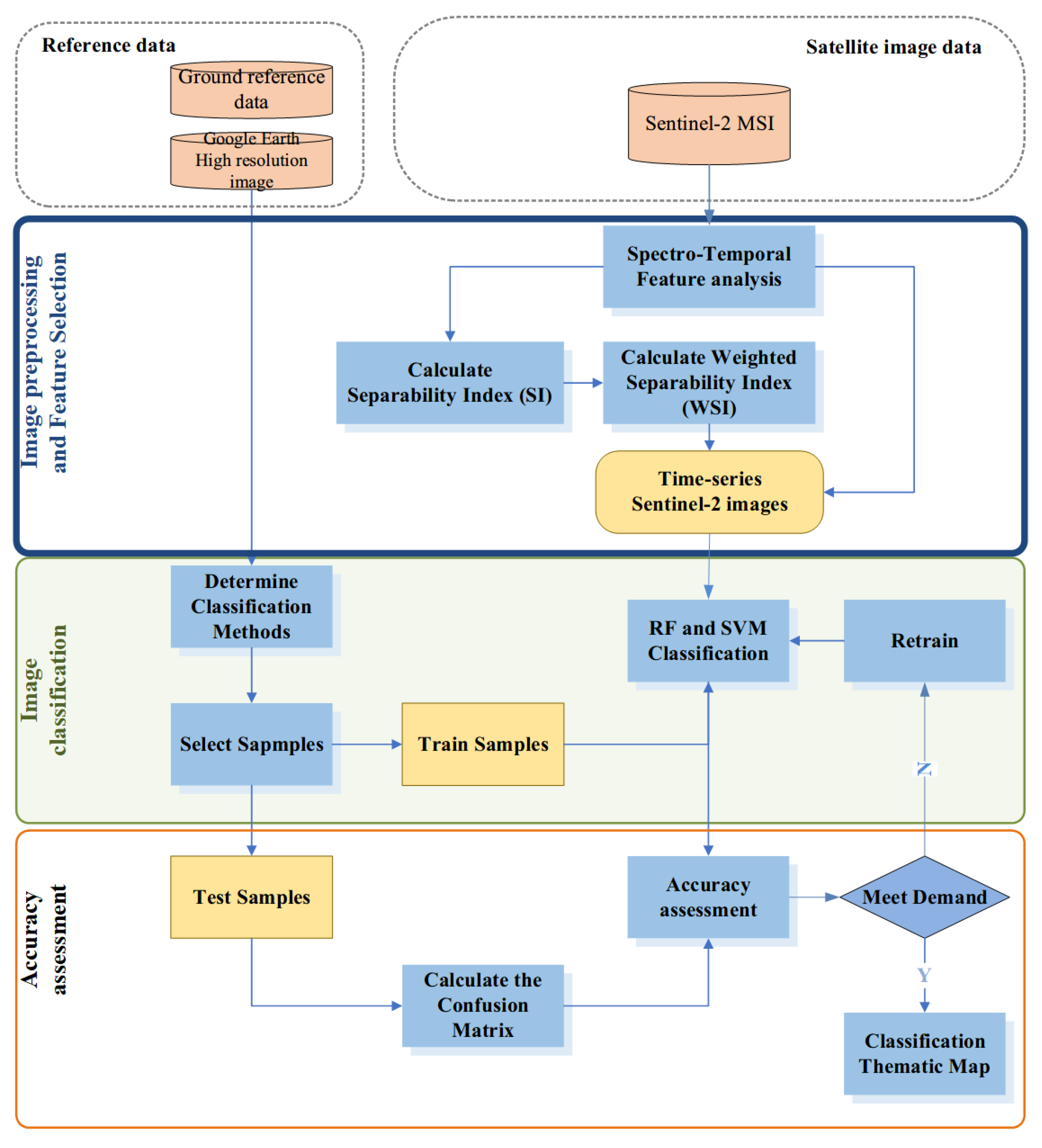
Based on the tropical forest classification mentioned above, we collected reference data (including training and validation samples) from the fieldwork and very-high-resolution imagery from Google Earth.

3. Method

Figure 3 shows the workflow adopted in this study, outlining the methods used as follows: data pre-processing, forest classification type determination, feature analysis, temporal data classification methods, and accuracy verification steps.

3.1. Pre-Processing

3.1.1. Cloud Mask

Considering that the southern coastal areas of China are covered by clouds all year round, we used the built-in “CLOUDY_PIXEL_PERCENTAGE” attribute of Sentinel-2 to remove pixels with cloud content greater than 20%. After that, the QA60 cirrus cloud band unique to Sentinel-2 was also used for cloud removal. After the above steps, we discriminated and removed cloud and cirrus pixels from each image.

3.1.2. Spectral Indices Calculation

Spectral Index (VI) can effectively reflect the degree of vegetation coverage on the Earth’s surface and the growth status of vegetation. Using VIS in remote sensing classification can help to enhance the ability of remote sensing interpretation and target recognition. We adopted the five spectral indices listed in

Table 2. Vegetation indices (VI) derived from Sentinel-2 imagery.

Vegetation Indices	Equations
NDVI	$\frac{NIR-RED}{NIR+RED}$
EVI	$2.5\ast \frac{NIR-RED}{NIR+6.0RED-7.5BLUE+1}$
NDTI	$\frac{SWIR1-SWIR2}{SWIR1+SWIR2}$
LSWI	$\frac{NIR-SWIR1}{NIR+SWIR2}$
SAVI	$(1.1-\frac{SWIR2}{2.0})\ast \frac{SWIR1-RED}{SWIR1+RED+0.1}$

. Given that Sentinel-2 imagery has both 10 m and 20 m bands, we resampled all of the 20 m Sentinel-2 bands to data with the spatial resolution of 10 m before calculating the above spectral indices.

3.2. Spectro-Temporal Feature Selection Method Based on the Weighted Separation Index

Somers and Asner [24] proposed the separability index (SI) (Formula (1)), which is defined as the ratio of the spectral difference inter- and intra-classes. Spectral differences inter- and intra-classes are used to measure whether the feature set can effectively distinguish different land use types [30]. The feature set that makes the most consistent internally and at the same time has the greatest difference between categories is the best [31]. In addition, SI does not require the research object to conform to the normal distribution, so its application range is wider than another commonly used index, separability Jeeries–Matusita (JM) distance [32]. Based on the above reasons, we chose SI to calculate the separability of three types of the tropical forests, and at the same time obtained the optimal feature set for classification:

$${\mathrm{SI}}_{\mathrm{ij}}(p,q)=\frac{\left|{\mu }_i-{\mu }_j\right|}{1.96\ast ({\sigma }_i+{\sigma }_j)}$$

(1)

where p represents a band or an index (a total of 10 in this study); q refers to a time point (a total of 6 in this study); ${\mu }_i$ and ${\mu }_j$ represent the mean spectral values of the samples of band or vegetation index p on date q for the class i (for example, tropical rainforest) and class j, respectively; ${\sigma }_i$ and ${\sigma }_j$ represent the standard deviation of the spectral values of the sample points of band or vegetation index p on date q for the class i and the class j, respectively. The absolute value of the difference between ${\mu }_i$ and ${\mu }_j$ can reflect the spectral difference between different classes, and the sum of the ${\mu }_i$ and ${\mu }_j$ can reflect the degree of dispersion and concentration of the spectrum within class i and class j. Based on Formula (1), it can be seen that the larger $\left|{\mu }_i-{\mu }_j\right|$ and smaller $({\sigma }_i+{\sigma }_j)$ will lead to a higher $S{I}_{ij}$ value. The higher $S{I}_{ij}$ is, the higher the separability of the two types of objects will be. In this paper, the SIs of three types of forest of the seven VIs and bands on six time periods were calculated. Finally, we obtained a total of 180 SIs.

However, the SI can only be used to calculate the pairwise separability between two types of ground objects and cannot reflect the overall separability between the three classes in this study. In order to solve this problem, we expanded each type of SI index by adding a weight, and the Weighted Separation Index (WSI) (Formula (2)) was extended:

$${\mathrm{WSI}}_{\mathrm{i}}(p,q)=\sum _j{w}_j{\mathrm{SI}}_{\mathrm{ij}}$$

(2)

where i represents the tropical forests type (for example, tropical rainforest); j represents the other types of the tropical forests (if i represents the tropical rainforest, the j represents the tropical monsoon forest or the evergreen broad-leaved forest); p represents a band or an index (a total of 10 in this study); q refers to a time point (a total of six in this study), $S{I}_{i}j$ is the SI calculated by Formula (1); and the $w_j$ represents the weight, which is calculated by the area ratio of the class j. These weights were calculated according to the classification results given in [29]. Compared with the direct selection of the average value of SI, the separability of features can be more objectively reflected by assigning different weights to different types of features in the form of area ratios.

3.3. Classifier

3.3.1. Random Forest Classifier

The RF algorithm has been applied to the classification of different types of satellite imagery successfully [33,34], since it is a very robust classifier. It is an algorithm that uses the theory of Ensemble Learning to integrate multiple trees. Therefore, its basic unit is the decision tree. In the forest composed of many independent decision trees, after random sampling from the original training data, each decision tree in a forest is used to judge the unmarked samples, and then the majority voting results of all decision trees are applied to predict the unmarked sample categories. The voting of each tree has the same weight. Previous studies demonstrated that the RF classifier has a fast training speed with high classification accuracy, as it is not sensitive to outliers and does not tend to over-fit easily [35,36]. In this research, the number of trees was set to 200, since previous studies have found that a number of trees larger than 120 creates a more stable accuracy for maps. For the other two parameters, we adopted the default values (the minimum number of terminal seeds: 1; the number of features: the square root of the number of all features) [37].

3.3.2. Support Vector Machine

Support Vector Machine (SVM) is a supervised non-parametric statistical learning technique, therefore, there is no assumption made on the underlying data distribution. In its original formulation [38], the method is presented with a set of labeled data instances. The SVM training algorithm aims to find a hyperplane that separates the dataset into a discrete predefined number of classes in a fashion consistent with the training examples. SVM is typically a supervised classifier, which requires training samples. Literature shows that SVM is not relatively sensitive to training sample size. Scientists have improved SVM to successfully work with limited quantity and quality of training samples [39].

3.4. Accuracy Assessment

The classification accuracy was quantitatively evaluated by applying validation samples. Based on tropical forests samples mentioned in Section 2.2.3, the locations of validation sample sites were determined by using a stratified random sampling. During the evaluation process, 70% of the samples were randomly selected for training the classifier, and the remaining 30% of the samples were used to verify the classification results.

A confusion matrix is calculated based on the sample data and classification result. Specific evaluation metrics include the Overall Accuracy ($OA$) (Formula (3)), the Kappa coefficient (Formula (4)), and the F1 measure [40]. The Kappa coefficient and OA are used to evaluate the overall classification result, and the F1 measure is used to evaluate the accuracy of each class by using the Producer’s Accuracy ($PA$) (Formula (5)) and User’s Accuracy ($UA$) (Formula (6)). The $PA$ is the probability that a pixel is correctly classified as a given class. The $UA$ is the probability that a pixel classified as a certain class in the map actually represents that class on the ground [40]. The F1 score is a useful index to assess class-level accuracy and is calculated from the harmonic mean between $PA$ and $UA$ for tropical forests as in Formula (7) [41]:

$$OA=\sum _{i=1}^k\frac{x_{ii}}{N}\times 100\%$$

(3)

$$K_a=\frac{N{\sum }_{i=1}^k{x}_{ii}-{\sum }_{i=1}^k{x}_{irow}{x}_{icol}}{N^2-{\sum }_{i=1}^k{x}_{irow}{x}_{icol}}$$

(4)

$$PA=\frac{x_{ii}}{x_{irow}}\times 100\%$$

(5)

$$UA=\frac{x_{ii}}{x_{icol}}\times 100\%$$

(6)

$$F1=\frac{2\times PA\times UA}{PA+UA}$$

(7)

where $x_{ii}$ represents the number of correctly classified samples in category i; N represents the total number of validation samples; $K_a$ is the Kappa coefficient; $x_{irow}$ and $x_{icol}$ are the sum of the elements of i row and i column in the confusion matrix, respectively.

4. Results

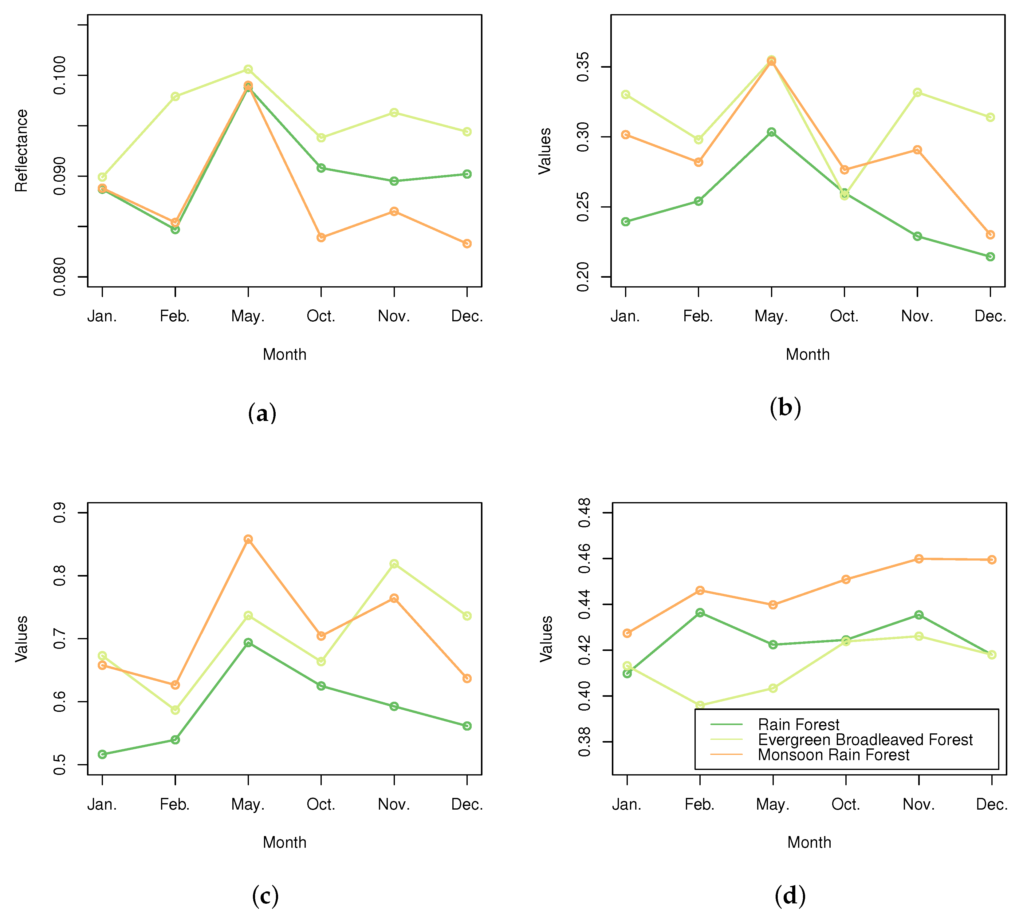
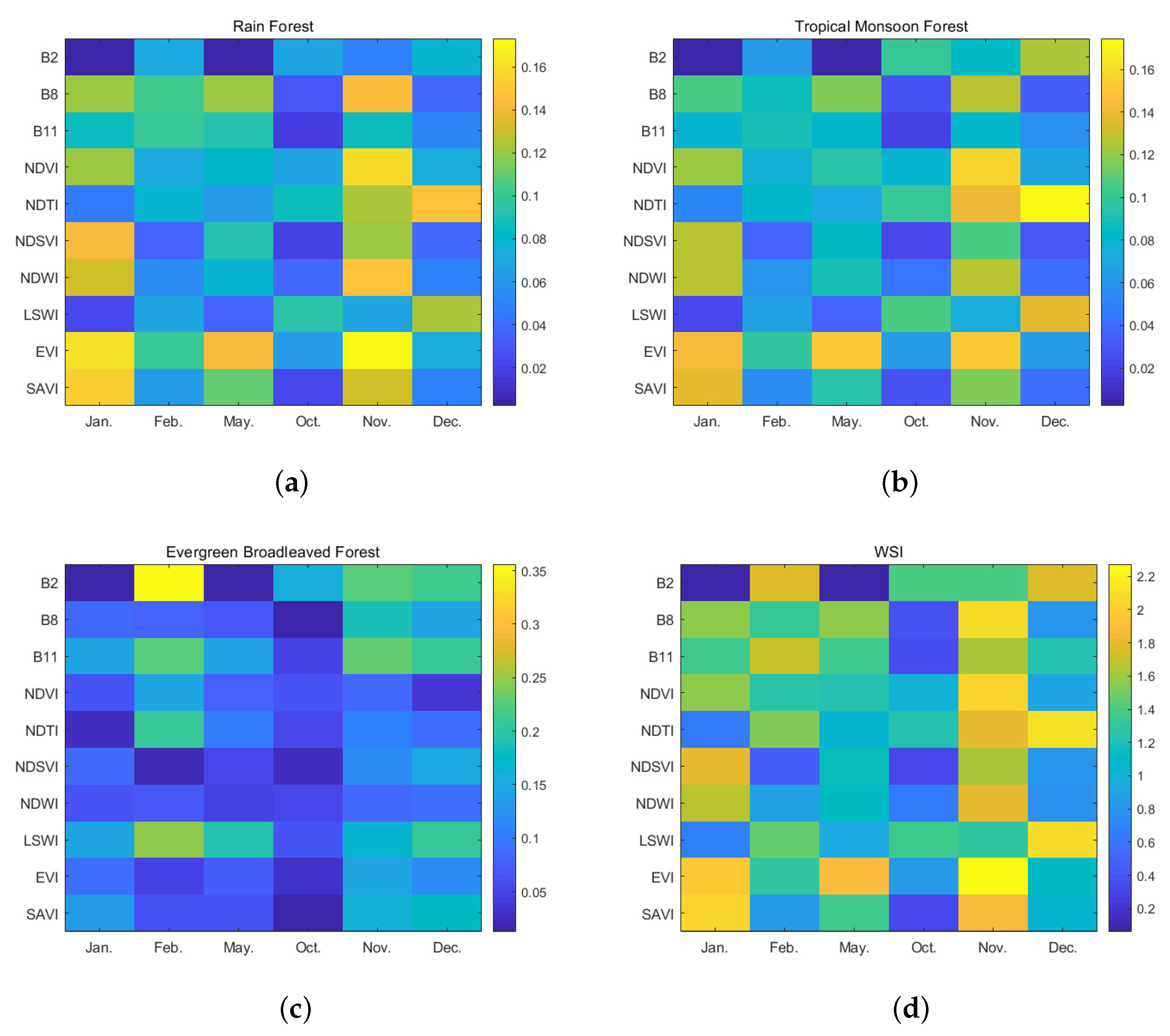
4.1. Spectro-Temporal Feature Analyses of Three Tropical Forests

Spectral differences existed among three types of tropical forests, but the difference was not obvious (Figure 4), which confirms the difficulty of distinguishing the three types of tropical forests. In the RED band, the curve of RF and MRF had a peak in the February, while the EBF continuously raised. There are differences between the three in winter. In the SAVI and EVI bands, the trends were basically the same. The RF was significantly lower than the others. The separability was better in the data of November and December. The NDTI curve of MRF was the highest and showed a continuous increasing trend, but other types experienced less fluctuation. Thus, the difference between three types of tropical forests could be distinguished in these indices and can be used for classification in this study.

4.2. Spectro-Temporal Feature Selection (STFS) Result

The separability indices for RF, EBF, TMF, and the WSI for the three types of tropical forests were shown in Figure 5 as the four matrices. The colors of grids in these matrices represented the different values of the SIs. The colors varied from blue to yellow, which corresponded to the values of indices from low to high. Through the matrices in Figure 5, we obtained the importance ranking of all spectro-remporal features. It was clear from the four matrices that the contribution of each spectro-remporal feature in classification was different. In terms of separating three types of tropical forests, as shown in Figure 5, the three spectral indices EVI, SAVI, and NDTI were the most important spectral features, and the three months January, November, and December were the most important temporal features.

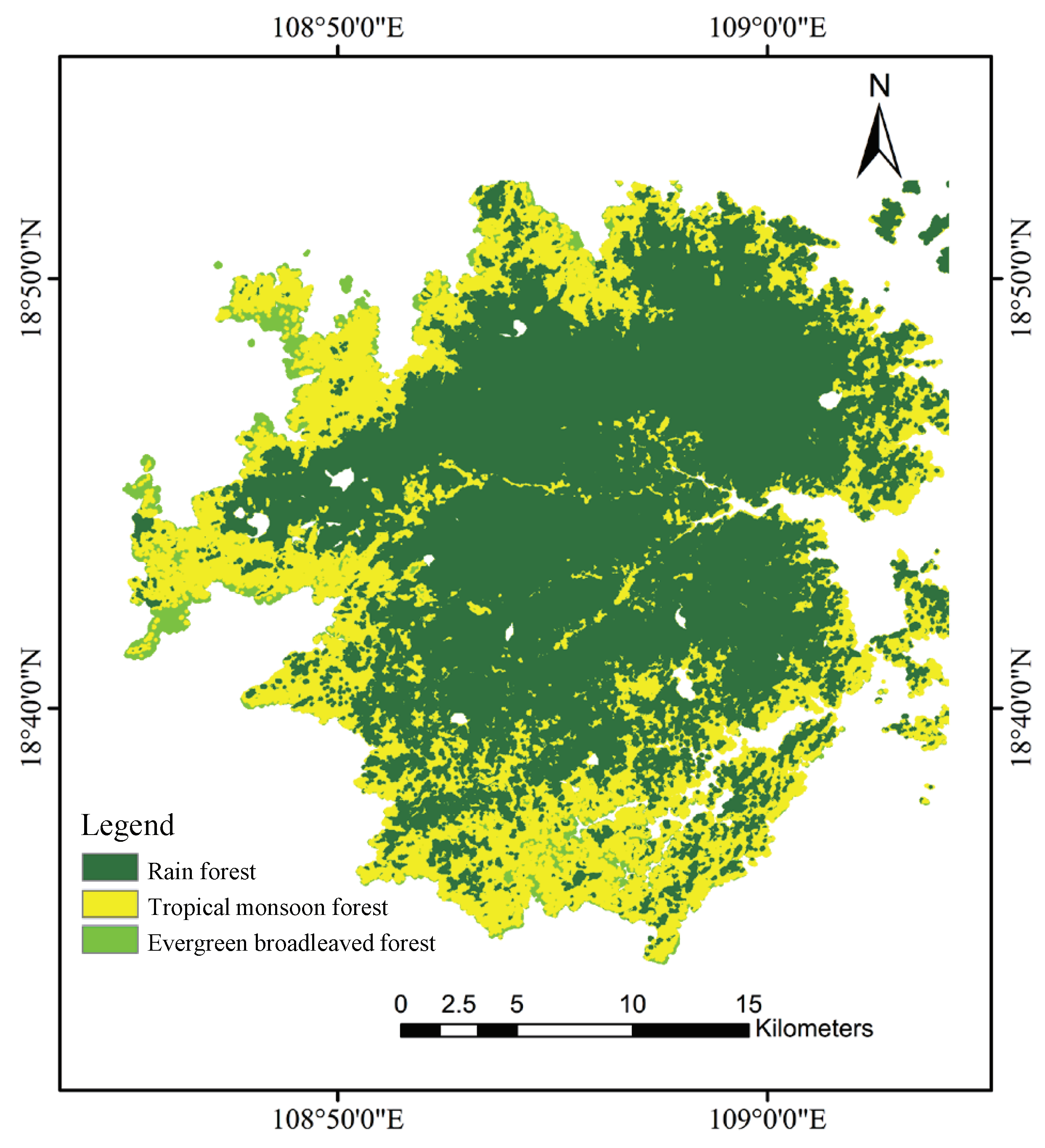
4.3. Tropical Forests Map in Jianfengling

As the produced thematic map resulting from temporally Sentinel-2 data revealed, the tropical forests map in Jianfengling is shown in Figure 6, showing the distribution of three types of tropical forests, including tropical rainforest, tropical monsoon forest, and evergreen broad-leaved forest. Some areas were masked because there were no cloud free observation images throughout the entire year. By comparing the classified result (Figure 6) with the field survey data, we found the classification result of the tropical natural forests obtained was reasonable.

Table 3. Confusion matrix of Tropical Forests Map in Jianfengling.

Classification	RF	TMF	EBF	$\mathbf{PA}$	F1
Rain forest (RF)	1844	87	35	93.79%	0.92
Tropical monsoon forest (TMF)	154	81	1553	84.86%	0.88
Evergreen broadleaved forest (EBF)	5	35	2363	98.31%	0.96
$UA$	92.06%	91.52%	95.24%	$OA=93.25\%$	$Kappa=90.08\%$

shows the confusion matrix of the three types of tropical forests obtained by the classifier. The overall accuracy reached 93.25%, and the Kappa coefficient was 0.90. The F1 measure of the three types of forests were 0.92, 0.88, and 0.96. For the tropical rainforest, the user’s accuracy and producer’s accuracy reached 93.79% and 92.06%, respectively. It was easy to distinguish it by using multi-temporal data, as it had obvious seasonal characteristics. The evergreen broad-leaved forest had the highest user’s accuracy and producer’s accuracy, which were 95.24% and 98.31%, respectively, because it could be easily distinguished from other tropical natural forests as it had obvious latitude distribution characteristics. However, as tropical monsoon forests and evergreen broad-leaved forests were often mixed together, the producer’s accuracy of the tropical monsoon forest was only 84.86%, which may be due to the similarity between the spectral characteristic curves (shown in Figure 4a).

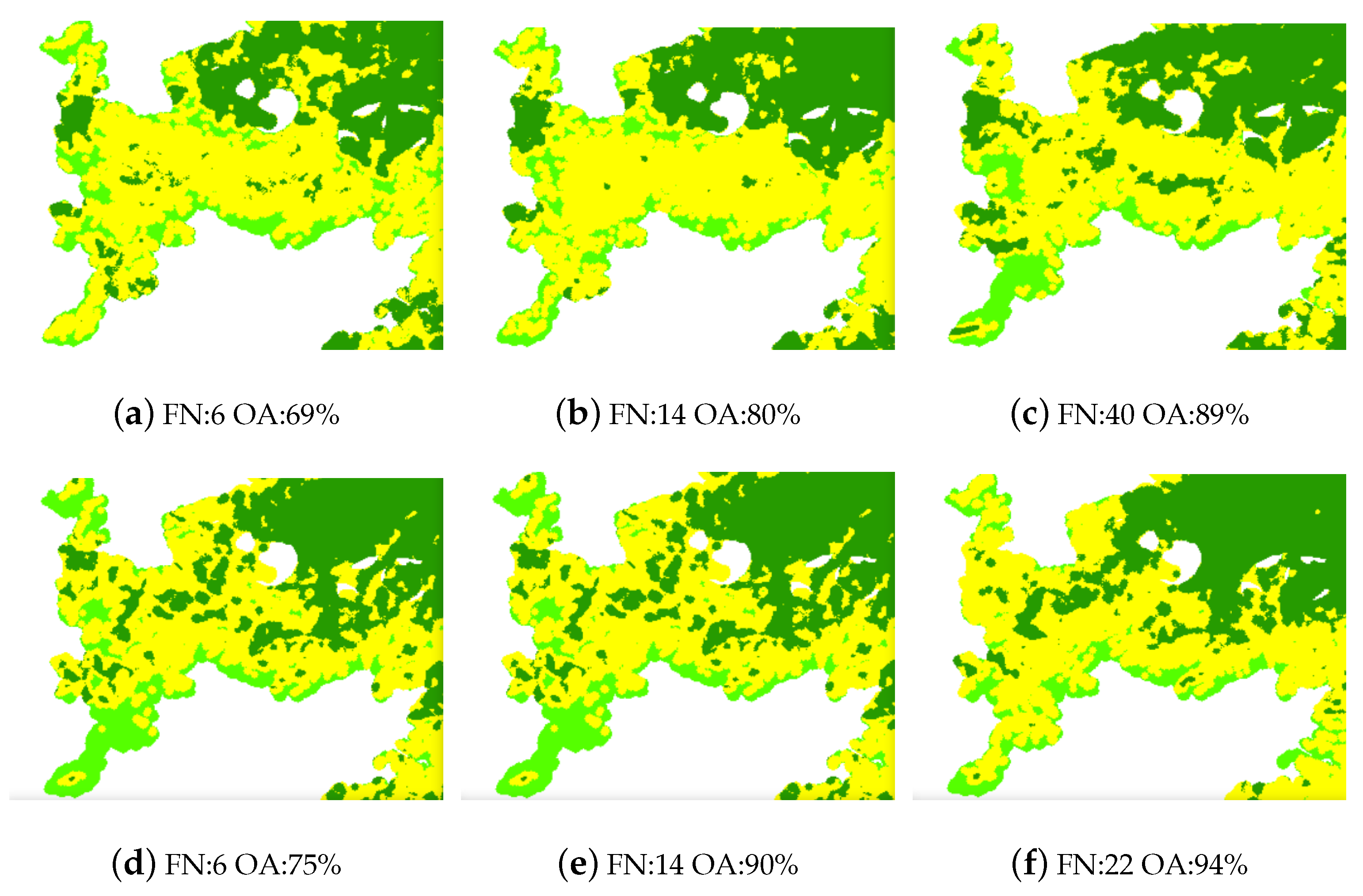
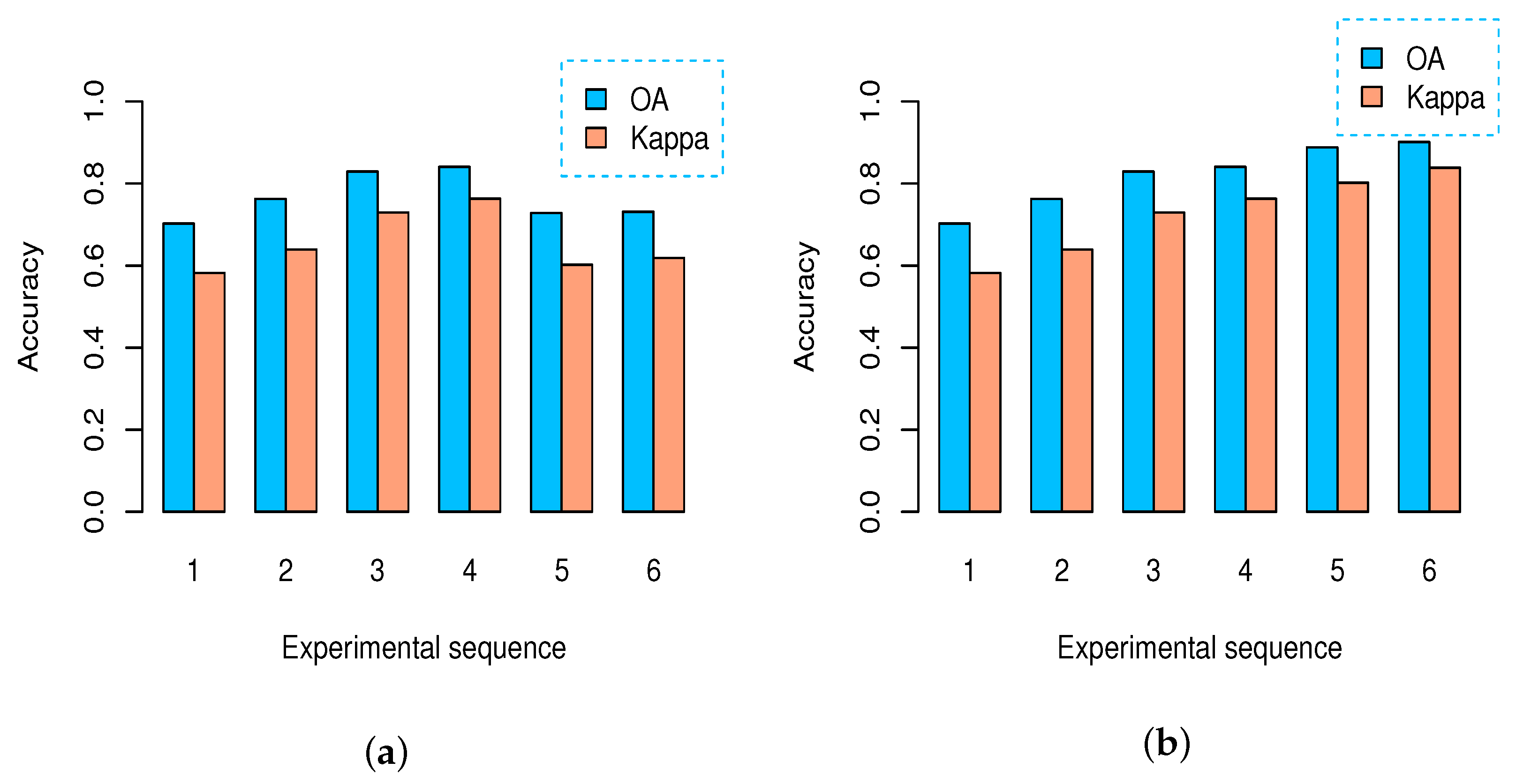
4.4. Comparison with the VSURF Method

In order to measure the improvement in the classification effect with the WSI method, we implemented Variable Selection Using Random Forest (VSURF) [18]. VSURF is a wrapper-based algorithm which used RF as the base classifier. As the VSURF algorithm was not implemented in GEE, the application of VSURF was performed in R software by their respective package implementations.

The accuracy of each classifier varied as a function of the type and the number of selected features. To explore the trend, we computed the overall accuracy (OA) for each suggested set of features, starting with the first four and incrementing by two until all variables were reached.

Figure 7a depicts the variability of OA based on the two FS methods (WSI and VSURF, respectively) suggested for the SVM classifier. The final classification accuracy of the two methods is similar (0.88), and when the number of features reaches a certain number (almost 30 this case), the accuracy reaches its peak and slightly fluctuates.

The result of the classification accuracy using the RF method is shown in Figure 7b. The WSI achieved better classification accuracy than VSURF in the RF classifier (0.94 and 0.89, respectively). RF appeared to be a robust classifier with respect to increasing feature space in this study as the accuracy of using the WSI had reached the optimal result.

5. Discussion

5.1. Performance of WSI-Based STFS Method

The study confirmed the utility of using the STFS method based on the WSI for mapping tropical forests at a fine scale. It can significantly reduce the number of features used in classification while ensuring classification accuracy. As shown in Figure 7a, when a small number of features are added in the early stage (when the number of features is from 6 to 28), the WSI-based STFS method can provide higher classification accuracy, which is 10% higher than the average VSURF added features. Moreover, to achieve a classification accuracy of 0.82, the STFS method requires 14 bands, while the VSURF requires 26 features. When faced with too many band features, the WSI can effectively remove redundant information and effectively improve classification accuracy and efficiency.

Figure 8 illustrated some details of two different FS methods using RF. The WSI based STFS method provided better classification accuracy than the VSURF method. When the number of features was six, the classification accuracy using the VSURF algorithm could only reach 69%, while the group using WSI could reach 75% (Figure 8a,b). When using the WSI method, tropical rainforests were more completely and accurately distinguished. The group using WSI reached 0.90 accuracy in OA with only a subset consisting of 14 features (Figure 8e), whereas VSURF achieved the highest accuracy with 0.89 and all 40 features (Figure 8c). The WSI method only used 35% of the total bands compared to VSURF but achieved almost the same classification accuracy.

Considering the classification accuracy trends, the WSI-based STFS method proved to be a more robust classifier to high dimensionality. Nonetheless, both algorithms made improvements over the full feature model with relatively small feature subsets.

5.2. The Impact of Bands Heterogeneity in Classification

This section mainly explores the impact of the number of bands on classification accuracy. Assuming that the above six phases of experimental data are obtained sequentially (that is, one phase of data is used for the first time, two phases of data are used for the second classification, and so on), the highest classification accuracy that can be achieved is studied separately. According to Section 4.2, the impact of each classification is obtained by calculating the WSI value of the period, and the top 14 features are selected for classification.

The final classification accuracy obtained is shown in Figure 9a. When the experimental data of the first four phases were added, the classification accuracy was steadily improved, but with the addition of the fifth and sixth phases, the classification accuracy decreased. Analyzing the classification characteristics, we found that some bands (such as B2, B11) have higher WSI values in different months, so the same bands (such as B2, B11) were added to the classifier multiple times. As a result, the number of bands used in subsequent classifications dropped significantly. Specifically, the different types of bands used in the first four periods of data are 10, 9, 8, and 8, respectively, while only 5 different bands were used in the fifth and sixth experiments.

In order to avoid this issue, when different time-series features of the same band appear more than twice in the classifier, we do not add the subsequent same features but instead use the remaining bands that have not been added to the classifier in order to maintain the diversity of features. The classification accuracy of the re-experiment is shown in the Figure 9b. With the elimination of redundant bands, the overall classification accuracy shows a trend of improvement as the amount of data increases, eventually reaching an extreme value of 0.90. Compared with the traditional multi-band and multi-feature classification, this experiment passed STFS screening and only selected 14 features to achieve the same classification accuracy as the 60 features, effectively saving computing power and cost.

5.3. Tropical Natural Forest Distribution in Hainsn Island

The focus of this section was to map the distribution of tropical forests. From the remote sensing classification results, the continuously distributed tropical forests occupied an area of roughly 605.6 ${\mathrm{km}}^2$, accounting for 94.6% of the total area of the Jianfengling research area.

For these different vegetation-type groups of tropical natural forests, tropical rainforests are mostly distributed in mountainous and relatively high-altitude areas, covering 404 ${\mathrm{km}}^2$. The tropical monsoon forests are basically distributed around the tropical rainforest, with an area of 178 ${\mathrm{km}}^2$. These two accounted for 66.7% and 29.4% of the tropical forests of Jianfengling, respectively. There are some evergreen broad-leaved forests scattered in the surrounding lower elevations, which are more susceptible to human influence.The distribution of various forests in the classification results is consistent with field and forestry survey data [42].

6. Conclusions

This paper mainly focuses on the inaccurate status of tropical forest classification, and the current needs for accurate identification and classification of tropical forest types in tropical areas. We rely on the GEE platform, using long-term remote sensing images to explore a complex terrain, multi-band, and multi-temporal tropical forest classification method. The main conclusions of this article are as follows.

The classification accuracy, combined with Sentinel-2 MSI data, the effects of multi-band spectral features, seven types of vegetation index (NDVI, EVI, NDTI, LSWI, SAVI, NDSVI, NDTI), and other features, is analyzed. The results show that as the number of bands with additional information increases, the classification accuracy continues to improve. Finally, the overall accuracy of the three types of features (tropical rainforest, tropical monsoon rainforest, and evergreen broad-leaved forest) reaches 0.88, and the total Kappa coefficient is 0.94. The distribution of tropical forests in Jianfengling area is obtained. Evergreen broad-leaved forests are mainly distributed in areas with low altitude and low humidity. Tropical monsoon forests are mainly distributed in middle- and high-altitude areas, while typical tropical rainforests are mainly distributed in high altitudes and high humidity, which have the largest area and are the dominant forest species in the forest.

The WSI-based STFS method used in this paper can be effective for feature selection when classifying massive data. The improvement is 10% higher than other feature selection methods, especially in the early stage of classification. It can achieve a better classification result by using a fewer feature subsets, which significantly reduces the cost of computing and time resources. We also find that it is not advisable to only pursue a higher WSI value in the classification process. In the actual process, the same waveband or vegetation index may have higher WSI attributes in different periods of time series images, which reduces the heterogeneity of wavebands. Therefore, it is necessary to take into account the heterogeneity and diversity of classification features.

In summary, the method developed in this paper using multi-band and multi-temporal remote sensing images based on WSI has effectively improved the classification accuracy of forest types represented by typical tropical rainforests, tropical monsoon forests, and evergreen broad-leaved forests. This method can effectively improve the classification accuracy of traditional tropical forest types and provide new methods and ideas for the fine classification of multi-temporal tropical forest types.

References

1. Aguilar, R.; Zurita-Milla, R.; Izquierdo-Verdiguier, E.; A De By, R. A cloud-based multi-temporal ensemble classifier to map smallholder farming systems. Remote Sens. 2018, 10, 729. [Google Scholar] [CrossRef] [Green Version]
2. Finer, M.; Babbitt, B.; Novoa, S.; Ferrarese, F.; Pappalardo, S.E.; De Marchi, M.; Saucedo, M.; Kumar, A. Future of oil and gas development in the western Amazon. Environ. Res. Lett. 2015, 10, 024003. [Google Scholar] [CrossRef]
3. Bonan, G.B. Forests and climate change: Forcings, feedbacks, and the climate benefits of forests. Science 2008, 320, 1444–1449. [Google Scholar] [CrossRef] [PubMed] [Green Version]
4. Baccini, A.; Goetz, S.; Walker, W.; Laporte, N.; Sun, M.; Sulla-Menashe, D.; Hackler, J.; Beck, P.; Dubayah, R.; Friedl, M.; et al. Estimated carbon dioxide emissions from tropical deforestation improved by carbon-density maps. Nat. Clim. Chang. 2012, 2, 182–185. [Google Scholar] [CrossRef]
5. Houghton, R.; Hall, F.; Goetz, S.J. Importance of biomass in the global carbon cycle. J. Geophys. Res. Biogeosci. 2009, 114. [Google Scholar] [CrossRef]
6. Pan, Y.; Birdsey, R.A.; Fang, J.; Houghton, R.; Kauppi, P.E.; Kurz, W.A.; Phillips, O.L.; Shvidenko, A.; Lewis, S.L.; Canadell, J.G.; et al. A large and persistent carbon sink in the world’s forests. Science 2011, 333, 988–993. [Google Scholar] [CrossRef] [PubMed] [Green Version]
7. Saha, N. Tropical Forest and Sustainability: An Overview; The Prince’s Charities’ International Sustainability Unit, Clarence House: London, UK, 2019. [Google Scholar]
8. Braatz, S. Sustainable Management of Forests and REDD+: Negotiations Need Clear Terminology; FAO: Rome, Italy, 2009. [Google Scholar]
9. Lawrence, D.; Vandecar, K. Effects of tropical deforestation on climate and agriculture. Nat. Clim. Chang. 2015, 5, 27–36. [Google Scholar] [CrossRef]
10. Kalamandeen, M.; Gloor, E.; Mitchard, E.; Quincey, D.; Ziv, G.; Spracklen, D.; Spracklen, B.; Adami, M.; Aragão, L.E.; Galbraith, D. Pervasive rise of small-scale deforestation in Amazonia. Sci. Rep. 2018, 8, 1–10. [Google Scholar] [CrossRef] [PubMed] [Green Version]
11. Potapov, P.; Dempewolf, J.; Talero, Y.; Hansen, M.; Stehman, S.; Vargas, C.; Rojas, E.; Castillo, D.; Mendoza, E.; Calderón, A.; et al. National satellite-based humid tropical forest change assessment in Peru in support of REDD+ implementation. Environ. Res. Lett. 2014, 9, 124012. [Google Scholar] [CrossRef]
12. Hansen, M.C.; Potapov, P.V.; Moore, R.; Hancher, M.; Turubanova, S.A.; Tyukavina, A.; Thau, D.; Stehman, S.; Goetz, S.J.; Loveland, T.R.; et al. High-resolution global maps of 21st-century forest cover change. Science 2013, 342, 850–853. [Google Scholar] [CrossRef] [Green Version]
13. Hansen, M.C.; Potapov, P.V.; Goetz, S.J.; Turubanova, S.; Tyukavina, A.; Krylov, A.; Kommareddy, A.; Egorov, A. Mapping tree height distributions in Sub-Saharan Africa using Landsat 7 and 8 data. Remote Sens. Environ. 2016, 185, 221–232. [Google Scholar] [CrossRef] [Green Version]
14. Huang, C.; Goward, S.N.; Masek, J.G.; Thomas, N.; Zhu, Z.; Vogelmann, J.E. An automated approach for reconstructing recent forest disturbance history using dense Landsat time series stacks. Remote Sens. Environ. 2010, 114, 183–198. [Google Scholar] [CrossRef]
15. Shimabukuro, Y.E.; dos Santos, J.R.; Formaggio, A.R.; Duarte, V.; Rudorff, B.F.T. The Brazilian Amazon monitoring program: PRODES and DETER projects. In Global Forest Monitoring from Earth Observation; Achard, F., Hansen, M.C., Eds.; CRC Press, Taylor & Francis Group: Boca Raton, FL, USA, 2012; pp. 153–169. [Google Scholar]
16. Hu, L.; Xu, N.; Liang, J.; Li, Z.; Chen, L.; Zhao, F. Advancing the mapping of mangrove forests at national-scale using Sentinel-1 and Sentinel-2 time-series data with Google Earth Engine: A case study in China. Remote Sens. 2020, 12, 3120. [Google Scholar] [CrossRef]
17. Hunt, M.L.; Blackburn, G.A.; Carrasco, L.; Redhead, J.W.; Rowland, C.S. High resolution wheat yield mapping using Sentinel-2. Remote Sens. Environ. 2019, 233, 111410. [Google Scholar] [CrossRef]
18. Genuer, R.; Poggi, J.M.; Tuleau-Malot, C. VSURF: An R package for variable selection using random forests. R J. 2015, 7, 19–33. [Google Scholar] [CrossRef] [Green Version]
19. Georganos, S.; Grippa, T.; Vanhuysse, S.; Lennert, M.; Shimoni, M.; Kalogirou, S.; Wolff, E. Less is more: Optimizing classification performance through feature selection in a very-high-resolution remote sensing object-based urban application. GISci. Remote Sens. 2018, 55, 221–242. [Google Scholar] [CrossRef]
20. Guyon, I.; Elisseeff, A. An introduction to variable and feature selection. J. Mach. Learn. Res. 2003, 3, 1157–1182. [Google Scholar]
21. Pal, M. Random forest classifier for remote sensing classification. Int. J. Remote Sens. 2005, 26, 217–222. [Google Scholar] [CrossRef]
22. Ghimire, B.; Rogan, J.; Galiano, V.R.; Panday, P.; Neeti, N. An evaluation of bagging, boosting, and random forests for land-cover classification in Cape Cod, Massachusetts, USA. GISci. Remote Sens. 2012, 49, 623–643. [Google Scholar] [CrossRef]
23. Gumus, E.; Kirci, P. Selection of spectral features for land cover type classification. Expert Syst. Appl. 2018, 102, 27–35. [Google Scholar] [CrossRef]
24. Somers, B.; Asner, G.P. Multi-temporal hyperspectral mixture analysis and feature selection for invasive species mapping in rainforests. Remote Sens. Environ. 2013, 136, 14–27. [Google Scholar] [CrossRef]
25. Xiao, D.; Long, Y.; Wang, S.; Fang, L.; Xu, D.; Wang, G.; Li, L.; Cao, W.; Yan, Y. Spatiotemporal distribution of malaria and the association between its epidemic and climate factors in Hainan, China. Malar. J. 2010, 9, 1–11. [Google Scholar] [CrossRef] [Green Version]
26. Drusch, M.; Del Bello, U.; Carlier, S.; Colin, O.; Fernandez, V.; Gascon, F.; Hoersch, B.; Isola, C.; Laberinti, P.; Martimort, P.; et al. Sentinel-2: ESA’s optical high-resolution mission for GMES operational services. Remote Sens. Environ. 2012, 120, 25–36. [Google Scholar] [CrossRef]
27. Xu, F.; Li, Z.; Zhang, S.; Huang, N.; Quan, Z.; Zhang, W.; Liu, X.; Jiang, X.; Pan, J.; Prishchepov, A.V. Mapping winter wheat with combinations of temporally aggregated Sentinel-2 and Landsat-8 data in Shandong Province, China. Remote Sens. 2020, 12, 2065. [Google Scholar] [CrossRef]
28. Song, Y.C.; Yan, E.R.; Song, K. An update of the vegetation classification in China. Chin. J. Plant Ecol. 2017, 41, 269. [Google Scholar]
29. Zhang, L.; Wan, X.; Sun, B. Tropical Natural Forest Classification Using Time-Series Sentinel-1 and Landsat-8 Images in Hainan Island. In Proceedings of the IGARSS 2019—2019 IEEE International Geoscience and Remote Sensing Symposium, Yokohama, Japan, 28 July–2 August 2019; pp. 6732–6735. [Google Scholar]
30. Yin, L.; You, N.; Zhang, G.; Huang, J.; Dong, J. Optimizing feature selection of individual crop types for improved crop mapping. Remote Sens. 2020, 12, 162. [Google Scholar] [CrossRef] [Green Version]
31. Hu, Q.; Wu, W.; Song, Q.; Yu, Q.; Lu, M.; Yang, P.; Tang, H.; Long, Y. Extending the pairwise separability index for multicrop identification using time-series modis images. IEEE Trans. Geosci. Remote Sens. 2016, 54, 6349–6361. [Google Scholar] [CrossRef]
32. Zhang, J.; Rivard, B.; Sánchez-Azofeifa, A.; Castro-Esau, K. Intra-and inter-class spectral variability of tropical tree species at La Selva, Costa Rica: Implications for species identification using HYDICE imagery. Remote Sens. Environ. 2006, 105, 129–141. [Google Scholar] [CrossRef]
33. Jin, Z.; Azzari, G.; You, C.; Di Tommaso, S.; Aston, S.; Burke, M.; Lobell, D.B. Smallholder maize area and yield mapping at national scales with Google Earth Engine. Remote Sens. Environ. 2019, 228, 115–128. [Google Scholar] [CrossRef]
34. Zurqani, H.A.; Post, C.J.; Mikhailova, E.A.; Schlautman, M.A.; Sharp, J.L. Geospatial analysis of land use change in the Savannah River Basin using Google Earth Engine. Int. J. Appl. Earth Obs. Geoinf. 2018, 69, 175–185. [Google Scholar] [CrossRef]
35. Rodriguez-Galiano, V.F.; Ghimire, B.; Rogan, J.; Chica-Olmo, M.; Rigol-Sanchez, J.P. An assessment of the effectiveness of a random forest classifier for land-cover classification. ISPRS J. Photogramm. Remote Sens. 2012, 67, 93–104. [Google Scholar] [CrossRef]
36. Zhong, L.; Gong, P.; Biging, G.S. Efficient corn and soybean mapping with temporal extendability: A multi-year experiment using Landsat imagery. Remote Sens. Environ. 2014, 140, 1–13. [Google Scholar] [CrossRef]
37. Hu, L.; Li, W.; Xu, B. Monitoring mangrove forest change in China from 1990 to 2015 using Landsat-derived spectral-temporal variability metrics. Int. J. Appl. Earth Obs. Geoinf. 2018, 73, 88–98. [Google Scholar] [CrossRef]
38. Noble, W.S. What is a support vector machine? Nat. Biotechnol. 2006, 24, 1565–1567. [Google Scholar] [CrossRef]
39. Mountrakis, G.; Im, J.; Ogole, C. Support vector machines in remote sensing: A review. ISPRS J. Photogramm. Remote Sens. 2011, 66, 247–259. [Google Scholar] [CrossRef]
40. Congalton, R.G. A review of assessing the accuracy of classifications of remotely sensed data. Remote Sens. Environ. 1991, 37, 35–46. [Google Scholar] [CrossRef]
41. Hurskainen, P.; Adhikari, H.; Siljander, M.; Pellikka, P.; Hemp, A. Auxiliary datasets improve accuracy of object-based land use/land cover classification in heterogeneous savanna landscapes. Remote Sens. Environ. 2019, 233, 111354. [Google Scholar] [CrossRef]
42. Miao, N.; Xu, H.; Moermond, T.C.; Li, Y.; Liu, S. Density-dependent and distance-dependent effects in a 60-ha tropical mountain rain forest in the Jianfengling Mountains, Hainan Island, China: Spatial pattern analysis. For. Ecol. Manag. 2018, 429, 226–232. [Google Scholar] [CrossRef]
Figure 1. The location of the Jianfengling study area and the Sentinel-2 image provided by GEE.
Sustainability 13 13348 g001
Figure 2. Sample photos of field data collection: (a) Tropical rainforest; (b) Evergreen broad-leaved forest; (c) Tropical monsoon forest.
Sustainability 13 13348 g002
Figure 3. The workflow of the study.
Sustainability 13 13348 g003
Figure 4. Time-phase spectral characteristic curve of typical features (The horizontal axis represents the month and the vertical axis represents the reflectance of the band or the value of the VIs): (a) RED; (b) SAVI; (c) EVI; (d) NDTI.
Sustainability 13 13348 g004
Figure 5. The SIs of different types of forests (The horizontal axes represent the different month and the vertical axes represent the 10 spectral bands or vegetation index) and WSI of three types: (a) SI of Rain Forest; (b) SI of Tropical monsoon forest; (c) SI of Evergreen broad-leaved forest; (d) WSI of three types.
Sustainability 13 13348 g005
Figure 6. Tropical Forests Map in Jianfengling, Hainan Province.
Sustainability 13 13348 g006
Figure 7. Relationship between OA, number of features based on WSI and VSURF methods for the SVM and RF classifier: (a) SVMl; (b) RF.
Sustainability 13 13348 g007
Figure 8. Classification results and accuracy with different feature number (FN): Figures (ac) are based on the VSURF method, while Figures (df) are based on the WSI method.
Sustainability 13 13348 g008
Figure 9. Classification accuracy result (The horizontal axis represents the order of experiments and the number of time series images, and the blue bar represents the classification accuracy): (a) Ignoring bands’ heterogeneity; (b) Considering bands’ heterogeneity.
Sustainability 13 13348 g009