Will Increasing Government Subsidies Promote Open Innovation? A Simulation Analysis of China’s Wind Power Industry

Abstract

Keeping open innovation both stable and sustainable can be difficult when it involves cooperation between large enterprises. Some empirical studies suggest that subsidy policies can play a positive role. This study addresses two key questions that follow from this observation: first, if the intensity of a subsidy policy is increased, can it play a greater role in strengthening the stability of cooperation between firms? Second, what other factors play a mediating role in this effect? Utilizing a dynamic game model, this paper analyses influential factors such as absorptive capacity, frequency of engagement and technical value on cooperative stability, and investigates the role of innovation policy in the process of cooperation through a random number-driven simulation. The findings indicate that only when the absorption capacity and technological value of both partners meet a certain threshold is the probability of positive cooperative behavior improved. Otherwise, increased subsidies tend to foster negative cooperative behavior instead.

1. Introduction

China’s economy is currently developing from a scale-driven model to one driven more by efficiency and innovation, and, as part of this transition, is in need of an open innovation (OI) model characterized by greater resource sharing [1,2,3] The adoption of open innovation models, such as Cisco’s influx of external resources and Tesla’s patent “outflow”, has enabled some multinational corporations (MNCs) to develop and maintain their global competitive advantages [4,5]. However, when the benefits of such initiatives fail to meet expectations, there is a tendency for companies to lose trust and exhibit selfish behavior, ultimately affecting the stability and sustainability of open innovation [6,7]. For example, when a wind turbine manufacturer and a blade producer cooperate to develop new types of blades, the two sides may fear each other’s capacity to absorb their core technologies and expertise, and thus carefully protect these resources from leaking to their partners. This distrust leads to less frequent discussions during the research and development (R&D) collaboration process, despite the necessity of consistent communication in designing the new wind turbines. This can ultimately lead to the end of the cooperation [8]. The identification of strategies for improving the stability and sustainability of cooperation in open innovation is an urgent need that must be addressed both theoretically and practically [9,10].

Based on these observations, this study investigates the effect of subsidy policies on the cooperation behavior of firms in the wind power industry (WPI). The WPI provides an excellent case as it is highly influenced by government policy in both emerging and developed economies [11]. It is also an industry which relies highly on R&D, and in which cooperative R&D between the industrial chain compartments is common. Typically, innovation in the WPI involves cooperation between separate companies producing blades, towers, generators, electrical controls, gearboxes, and wind farms. China’s WPI in particular has been described as characterized by strong links between companies along the industrial chain, the key significance of R&D activities, and a high level of policy influence.

Game theory offers a useful approach to understanding how innovative entrepreneurial behavior at the micro-level both drives and responds to policies at the macro-level, in contrast to the common assumption that influence flows one way from macro-level policies to micro-level behavior [12]. This paper introduces random number simulation to the game theory approach in order to compare the effect of a range of potential subsidy policies. This approach helps identify the conditions under which innovation policy exerts the most beneficial effect.

The Section 2 of this paper defines the concept of open innovation, describes its operational processes, and analyzes the influence of the absorptive capacity of enterprises, the frequency of cooperation among enterprises, and the value of resources on stability and sustainability of cooperation. The Section 3 analyzes the interaction between innovation partners given different scenarios using a non-cooperative game equilibrium model. The Section 4 presents the results of a simulation of the behavior of enterprises and their corresponding innovative output under different subsidy conditions.

2. Theoretical Background and Hypotheses

2.1. Theoretical Fundamentals

Previous research seeking ways to improve performance in open innovation has generally taken one of two perspectives: micro-level enterprise strategy or macro-level policy formulation. The micro-level perspective focuses on the dimension of enterprise choice and operates from the belief that enterprises can adopt a strategy of minimizing loss and maximizing exclusive intellectual property [13,14,15,16]. The macro-level approach focuses on improving policy instruments such as infrastructure, tax incentives, and financial support [17,18,19,20]. From a macro-level perspective, government R&D subsidies are expected to have a positive effect on innovative activities in the renewable energy industry because they help to reduce uncertainties. Research indicates that R&D subsidies promote incremental, predictable, and credible expenditures that facilitate the development of renewable energy technology [21], and that public R&D and tariff incentives are significant instruments for increasing international trade as well as domestic R&D [22]. Besides, public policy must create open innovation environments accordingly with the quintuple helix harmonizing the ecosystem to internalize emerging spillovers [23].

Recent research suggests the need to combine the micro- and macro-level perspectives to address the interplay between policy instruments and enterprise behavior and to understand innovation systems holistically [24,25]. For example, some studies have investigated the effect of renewable energy policy on technological innovation systems [26,27,28], while others have analyzed the structure of innovation systems to identify starting points for policy intervention and explain the success or failure of R&D and diffusion [28,29,30]. This emerging holistic focus recognizes the relationship between the whole and the parts of innovation systems [31,32]. Despite this trend, however, research continues to ignore the driving factors of cooperation and technological innovation, and the influence of policy on cooperative behavior [33]. Open innovation (OI) is a process of interaction, overflow, and creation involving enterprises, governments, research institutions, universities, and intermediary organizations. Policy plays a role in guiding the direction innovation takes, allocating resources for innovation, and stimulating innovative cooperation. However, it may function differently in different situations. For instance, in the early 2000s, an R&D policy was developed to promote cooperation between enterprises in Germany. A cooperative atmosphere gradually formed in response, and the technological level of wind power and other renewable energy industries rapidly increased [34]. In contrast, the Non-Fossil Fuel Obligation (NFFO) policy in the UK has not succeeded in encouraging cooperative innovation among enterprises. Rather, it encourages independent technological R&D and inadvertently sets barriers to industrial entry [35]. Therefore, in order to formulate targeted and efficient policy tools, it is necessary to analyze responses to government policies and determine the optimal cooperation conditions for innovation systems [36,37].

2.2. Open Innovation Processes in the Wind Power Industry

Tucci et al. [7] define OI as a distributed innovation process in which an organization intentionally manages the flow of knowledge at its own boundaries through monetary and non-monetary mechanisms. Wind power is an emerging strategic industry that is in a high growth stage, characterized by closed technical links in the industrial chain, asset specificity, and constant technological advancement. Therefore, current common practice across countries is to promote the development of common technologies through subsidy policies and the use of open innovation platforms [38].

The innovation model of China’s WPI has evolved from closed, independent R&D through innovation based on imitation and cooperation to open innovation [39]. In recent years, wind turbine manufacturers, component makers, and ancillary enterprises have engaged in seamless processes of shared innovation, cooperating to produce solutions customized to specific project contexts at every stage from initial supply to final wind farm design.

OI is an organic process requiring high levels of participation, trust, and communication. In the wind power industry, for instance, innovation cooperation typically occurs between wind turbine control system enterprises (A) and blade manufacturing enterprises (B). A’s advantage lies in the lifecycle management of intelligent control systems and smart wind farms, while B’s is in its accumulated experience in producing composite materials and in process and structure design.

When two companies like this work together to develop new products, A generally designs the aerodynamic profile of the blades while B is responsible for their structural design. Information leaks during this kind of cooperation may weaken an enterprise’s competitive advantage in the future [40]. Therefore, companies always attempt to regulate the flow of information through technical cooperation agreements.

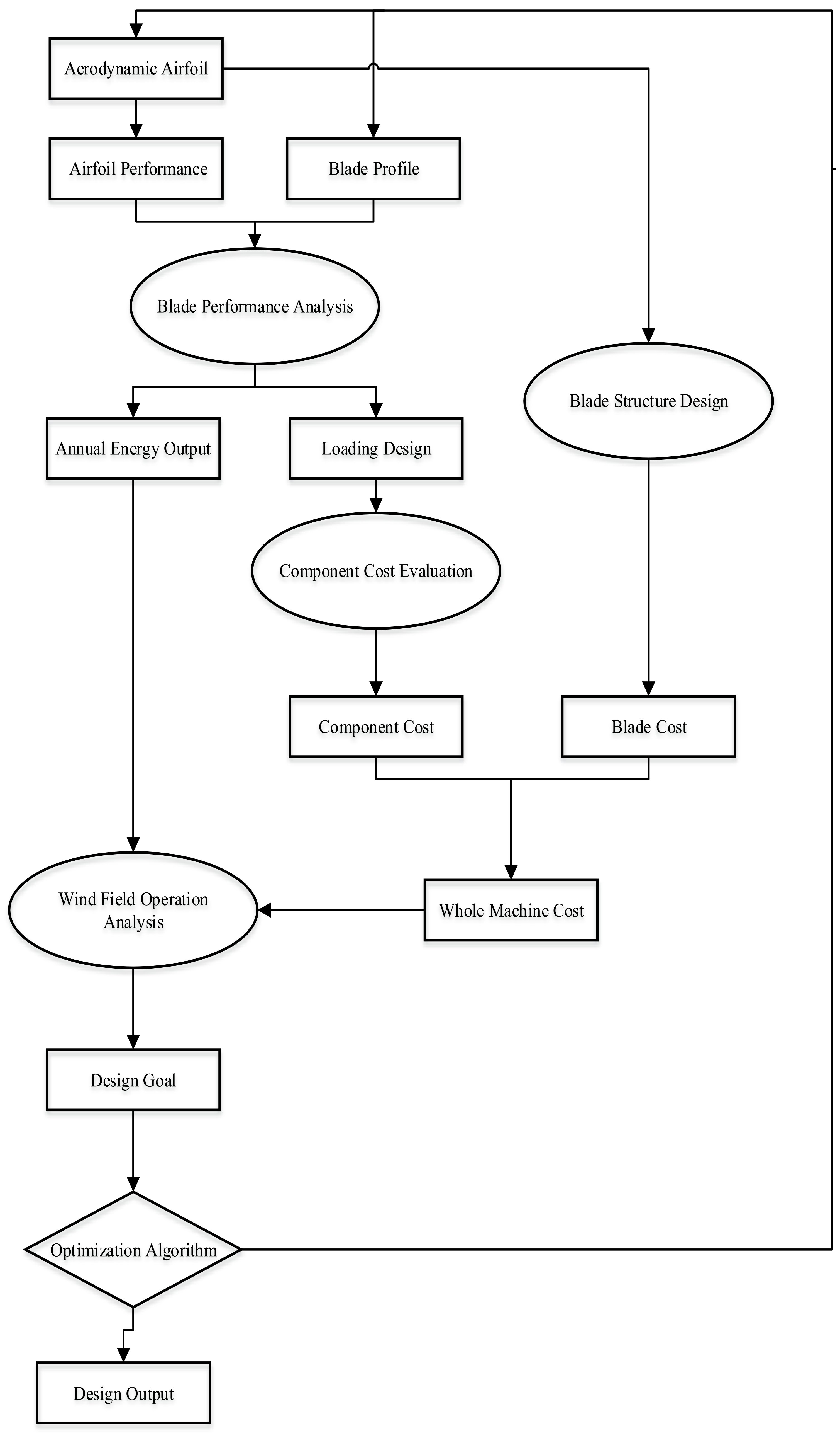
A and B each have strengths that address the other’s weaknesses, and there is a desire on both sides to share expertise. A wants B to share process drawings and structural calculations, while B wants A to share blade designs and input parameters. Trust-based negotiation is necessary, and may result, for example, in an agreement between the two sides which states that the products of the joint development cannot be sold to third parties for a specified period. The cooperation agreement will also typically draw a clear distinction between “background technology”, owned separately by each enterprise prior to their cooperation, and the “long-term technology” resulting from their cooperation. This case, as an illustration, is summarized in Figure 1.

Both sides in this case seek to maximize their own interests and make decisions to further these interests based on incomplete information [41]. In order to maintain control of their own technology, enterprises selectively disclose information [42] when forming an innovative cooperative relationship with a benefit-sharing mechanism [43]. Innovation activities are uncertain processes, and this uncertainty is exacerbated by any instability in the cooperation.

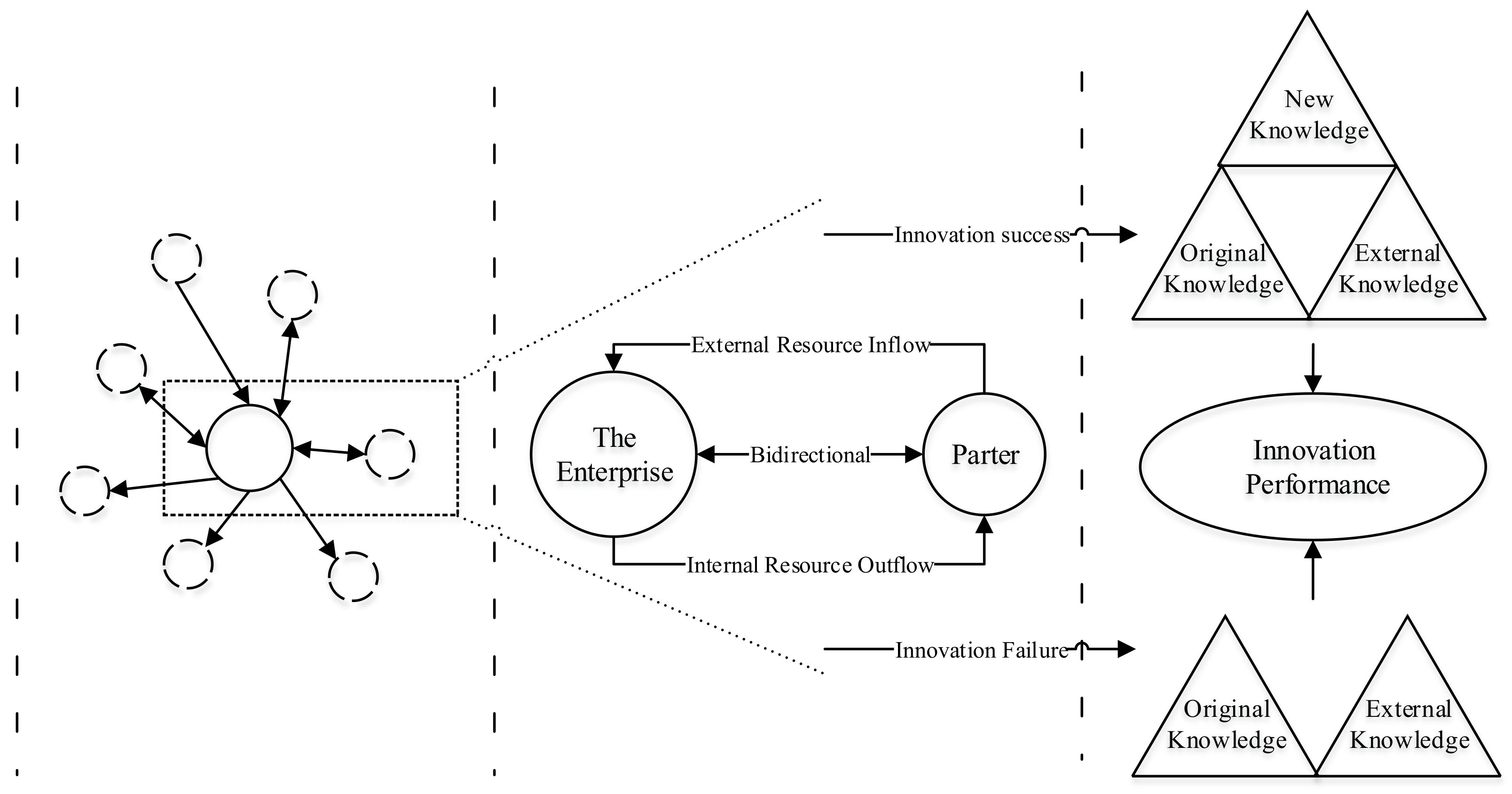
As shown in Figure 2, the process of open innovation involves: (1) outflow of internal resources such as capital, technology, knowledge, and information; (2) inflow of external resources; and (3) bidirectional flow of resources between the focal enterprise and its partners. Companies innovate through integration of their own resources with externally acquired resources, and develop market opportunities to increase the benefits of innovation through this integration. If an enterprise cannot integrate its own resources with externally acquired resources, it fails to benefit from cooperation and OI will be difficult to sustain.

2.3. Research Hypotheses

OI’s potential to enhance adaptability and innovation depends on the coordination between the partners [44]. Although OI can enhance knowledge exchange among enterprises and improve innovation performance, the cooperation involved is often unstable. Each partner’s absorptive capacity, along with the frequency and technical value of cooperative activities, can affect future cooperative behavior. In turn, these elements thus determine the stability, sustainability, and success of a cooperative partnership. “Absorptive capacity” refers to the ability of an enterprise to identify, absorb, utilize, and assimilate knowledge gained through collaboration [45,46]. Absorptive capacities depend on the extent to which the cooperating companies’ knowledge bases resemble and complement each other [47]. Absorptive capacity impacts effective communication, integration, and coordination among companies, which affects the foundation of mutual trust and the willingness to share knowledge. A more recent study by Kim et al. [48] confirms that absorptive capacity is an important factor affecting the stability of cooperation.

Frequency of cooperation also affects the degree of mutual understanding and trust among enterprises [49,50]. Frequent cooperation can effectively inhibit the moral hazard of both parties and make the cooperation between the two more stable, since the two parties must cooperate several times over a certain period in order to achieve their shared R&D goals. This means only when they cooperate nicely this time that can ensure the probability of next-time cooperation. Besides, frequent cooperation allows more understanding between each other and enhances the commitment of two sides.

If the knowledge and technologies being collaborated on are the basis of the enterprises’ core competitiveness, this may also affect the openness and depth of cooperation. Where high-value knowledge is involved, concerns regarding technology leakage are more significant, and protectionism tends to impede cooperation. Absorptive capacity plays a role here as well; the stronger the absorptive capacity of the partners, the greater the fear that the absorption of core technology by partners will affect reduce market competitiveness.

Based on the above discussion, the following two hypotheses emerge:

Hypothesis 1 (H1).

The weaker the absorptive capacity of the partners during occasional cooperation, the more willing the enterprises will be to adopt an active cooperation strategy.

Hypothesis 2 (H2).

In the context of frequent cooperation among enterprises with strong absorptive capacity, positive and lasting cooperation can only be achieved when the outflow of the future value of the cooperative enterprises technology to each other are small enough.

Open innovation in emerging industries has a higher probability of failure and higher costs compared with that in established industries, which may dampen enthusiasm for this kind of cooperation. Policy incentives such as subsidies are needed to compensate for this. Between 2000 and 2015, the United States federal government provided companies with a total of at least 68 billion USD in grants, tax credits, etc. to encourage innovation, with 582 large companies accounting for 67% of this total [51]. In 2017, the German federal government provided nearly 36 billion EUR in debt repayment assistance, loans, investment subsidies, etc. to German companies to support the innovation [52]. China has also used industrial innovation policies to induce, coordinate, and guarantee the innovative behavior of enterprises in the industry. These policies have stimulated a rapid increase in the scale of wind power and other renewable energy sectors in China.

Although all parties (i.e., government, companies, and researchers) fundamentally agree on the necessity of R&D subsidies, there are contradictory findings on the question of whether R&D subsidies policy fully mitigate market failures [53,54]. Zúñiga-Vicente et al.’s [55] meta-analysis of relevant literature indicates that 63% of studies support the conclusion that R&D subsidies have effectively promoted the growth of enterprise R&D expenditures, but over one-third of studies indicate that subsidies have either no effect on R&D expenditure or a negative “crowding out” effect.

China’s R&D subsidy intensity is relatively low compared to that seen in the United States and many European countries [56]. It is likely that R&D subsidies may increase as overall R&D investment among Chinese businesses increases. Given the inconsistent findings reported above, however, it is unlikely that subsidy intensity alone can predict effectiveness in encouraging enterprises to innovate. Instead, the results will be determined by the specific policies put into place and how businesses and other actors respond to these policies. The goals of the government and private enterprise may deviate at times, as R&D funding policy is unable to fully meet all the specific needs of micro-actors. Policy impacts can thus become distorted in the process of cooperation in an open innovation system.

Therefore, we propose:

Hypothesis 3 (H3).

The effect of government subsidy policies on innovation performance depends on enterprises’ absorptive capacity and the new technological value to be obtained.

Section 3 below outlines our development of game theory models based on these three hypotheses.

3. Model Development

3.1. The Model and Its Components

3.1.1. Modeling Actors’ Behavior in the Absence of Policy Supports

Using the example of the wind turbine control system enterprise (A) and blade manufacturing enterprise (B) discussed in Section 2 above, we can establish a model in which they cooperate using their existing technologies as inputs. These technologies have value, both now and in the future.

The present value of the technical resources to the two enterprises is denoted as $V_0^i,i=\left\{A,B\right\}$ and the future value as $V_f^i,i=\left\{A,B\right\}$. Since the value of new technology comes from the input of existing technology, the value of new technology is:

$$V^{N_A}=V_0^A+V_0^B+V_0^A{V}_0^B+V_f^{N_A}$$

$$V^{N_B}=V_0^A+V_0^B+V_0^A{V}_0^B+V_f^{N_B}$$

where $V_0^A{V}_0^B$ represents the non-linear cooperation output [57]; and $V_f^{N_i},i=\left\{A,B\right\}$ represents the value of the new technology to the two companies in the future.

The absorptive capacity of the two businesses is represented by ${\beta }^i,i=\left\{A,B\right\};p$ is the probability of successful open innovation, and $V_f^{N_i}, i=\left\{A,B\right\}$ is a stochastic variable that produces a random fluctuation in open innovation performance. The expected net output of the two firms’ open innovation (hereinafter referred to as “open innovation gain”) is:

$${\pi }_0^A=p{V}^{N_A}-{\beta }^B{V}_f^A+{\beta }^A{V}_f^B=p\left(V_0^A+V_0^B+V_0^A{V}_0^B+V_f^{N_A}\right)-{\beta }^B{V}_f^A+{\beta }^A{V}_f^B$$

$${\pi }_0^B=p{V}^{N_B}-{\beta }^A{V}_f^B+{\beta }^B{V}_f^A=p\left(V_0^A+V_0^B+V_0^A{V}_0^B+V_f^{N_B}\right)-{\beta }^A{V}_f^B+{\beta }^B{V}_f^A$$

(1) Occasional cooperation model

In this model, companies A and B both prioritize their own interests in the cooperation. The business strategy space is set as $S_i=\left\{s_H, s_L\right\},\mathrm{where}{s}_H$ represents positive cooperation and $s_L$ denotes negative cooperation. Technical input is $\overline{V_0^i},\mathrm{and}$ the future value is $\overline{V_f^i};(\overline{V_0^i}>\underset{¯}{V_0^i},\overline{V_f^i}>\underset{¯}{V_f^i},i=\left\{A,B\right\}|)$. The business strategy portfolios and their returns are illustrated in

Table 1. Enterprise strategy portfolios and their returns.

		$\mathit{B}$
		${\mathit{s}}_{\mathit{H}}$		${\mathit{s}}_{\mathit{L}}$
$A$	$s_H$	$U_{HH}$	$W_{HH}$	$U_{HL}$	$W_{LH}$
	$s_L$	$U_{LH}$	$W_{HL}$	$U_{LL}$	$W_{LL}$

.

When both enterprises engage in positive cooperation behaviors $\left\{s_H,s_H\right\}$, the future value of the new technology obtained is higher, which is denoted as $\overline{V_f^{N_i}}$. When both engage in passive cooperation behaviors $\left\{s_L,s_L\right\}$, the future value of the new technology obtained is lower, which is denoted as $V_f^{N_i}$. When the two enterprises engage in different behaviors $\left\{s_H,s_L\right\}$, the future value of the new technology obtained is between the former two values, which is denoted as $\widetilde{V_f^{N_i}},i=\left\{A,B\right\}$. Thus, the matrixes for the two enterprises’ OI benefits are:

$${\pi }^A=\left[\begin{array}{cc}{U}_{HH}& U_{HL}\\ U_{LH}& U_{LL}\end{array}\right]$$

$$=\left[\begin{array}{cc}p\left(\overline{V_0^A}+\overline{V_0^B}+\overline{V_0^A}\overline{V_0^B}+\overline{V_f^{N_A}}\right)-{\beta }^B\overline{V_f^A}+{\beta }^A\overline{V_f^B}& p\left(\overline{V_0^A}+\underset{¯}{V_0^B}+\overline{V_0^A}\underset{¯}{V_0^B}+\widetilde{V_f^{N_A}}\right)-{\beta }^B\overline{V_f^A}+{\beta }^A\underset{¯}{V_f^B}\\ p\left(\underset{¯}{V_0^A}+\overline{V_0^B}+\underset{¯}{V_0^A}\overline{V_0^B}+\widetilde{V_f^{N_A}}\right)-{\beta }^B\overline{V_f^A}+{\beta }^A\underset{¯}{V_f^B}& p\left(\underset{¯}{V_0^A}+\underset{¯}{V_0^B}+\underset{¯}{V_0^A}\underset{¯}{V_0^B}+\underset{¯}{V_f^{N_A}}\right)-{\beta }^B\underset{¯}{V_f^A}+{\beta }^A\underset{¯}{V_f^B}\end{array}\right]$$

$${\pi }^B=\left[\begin{array}{cc}{W}_{HH}& W_{LH}\\ W_{HL}& W_{LL}\end{array}\right]$$

$$=\left[\begin{array}{cc}p\left(\overline{V_0^A}+\overline{V_0^B}+\overline{V_0^A}\overline{V_0^B}+\overline{V_f^{N_B}}\right)-{\beta }^A\overline{V_f^B}+{\beta }^B\overline{V_f^A}& p\left(\overline{V_0^A}+\underset{¯}{V_0^B}+\overline{V_0^A}\underset{¯}{V_0^B}+\widetilde{V_f^{N_B}}\right)-{\beta }^A\underset{¯}{V_f^B}+{\beta }^B\overline{V_f^A}\\ p\left(\underset{¯}{V_0^A}+\overline{V_0^B}+\underset{¯}{V_0^A}\overline{V_0^B}+\widetilde{V_f^{N_B}}\right)-{\beta }^A\overline{V_f^B}+{\beta }^B\underset{¯}{V_f^A}& p\left(\underset{¯}{V_0^A}+\underset{¯}{V_0^B}+\underset{¯}{V_0^A}\underset{¯}{V_0^B}+\underset{¯}{V_f^{N_B}}\right)-{\beta }^A\underset{¯}{V_f^B}+{\beta }^B\underset{¯}{V_f^A}\end{array}\right]$$

Set up:

$$V_{HH}^{N_A}=\overline{V_0^A}+\overline{V_0^B}+\overline{V_0^A}\overline{V_0^B}+\overline{V_f^{N_A}}, V_{HL}^{N_A}=\overline{V_0^A}+\underset{¯}{V_0^B}+\overline{V_0^A}\underset{¯}{V_0^B}+\widetilde{V_f^{N_A}},$$

$$V_{LH}^{N_A}=\underset{¯}{V_0^A}+\overline{V_0^B}+\underset{¯}{V_0^A}\overline{V_0^B}+\widetilde{V_f^{N_A}},V_{LL}^{N_A}=\underset{¯}{V_0^A}+\underset{¯}{V_0^B}+\underset{¯}{V_0^A}\underset{¯}{V_0^B}+\underset{¯}{V_f^{N_A}};$$

$$V_{HH}^{N_B}=\overline{ V_0^A}+\overline{V_0^B}+\overline{V_0^A}\overline{V_0^B}+\overline{V_f^{N_B}, }{V}_{LH}^{N_B}=\overline{V_0^A}+\underset{¯}{V_0^B}+\overline{V_0^A}\underset{¯}{V_0^B}+\widetilde{V_f^{N_B}},$$

$$V_{HL}^{N_B}=\underset{¯}{ V_0^A}+\overline{V_0^B}+\underset{¯}{V_0^A}\overline{V_0^B}+\widetilde{V_f^{N_B}},V_{LL}^{N_B}=\underset{¯}{V_0^A}+\underset{¯}{V_0^B}+\underset{¯}{V_0^A}\underset{¯}{V_0^B}+\underset{¯}{V_f^{N_B}}.$$

Proposition 1.

If${\beta }^i<min\left(\left(V_{HH}^{N_j}-V_{LH}^{N_j}\right)/\left(\overline{V_f^j}-\underset{¯}{V_f^j}\right)·p, \left(V_{HL}^{N_j}-V_{LL}^{N_j}\right)/\left(\overline{V_f^j}-\underset{¯}{V_f^j}\right)·p\right)$,$i, j=\left\{A, B\right\} and i\ne j$, then$s_L$is the dominant strategy of enterprise$B$.

Proposition 1 is demonstrated in Appendix A. This proposition relates to hypothesis H1 and illustrates that the weaker the absorptive capacity of the partners during occasional cooperation, the more willing the enterprises are to adopt an active cooperation strategy. Thus, the mode of cooperation between large core enterprises and small-scale suppliers in the industrial chain, compared with that between large enterprises, is simpler but more capable of generating technical cooperation. Although there are complicated business models among enterprises of similar sizes, it is often difficult for them to cooperate in practice, as noted by Diestre and Rajagopalan [58]. This phenomenon stems from the self-interest of enterprises as well as fears that the absorption of technology by partners will affect the exclusiveness of their technical value and reduce their market competitiveness.

(2) Multiple cooperation model

We use an infinite repeated game G (∞, δ) to model a situation in which both enterprises seek to maximize their own interests. Suppose that firms have the same time preference, and the discount rate for the future value is common to all firms, defined as δ (0 < δ < 1). Also, suppose that at any given game stage t, all firms can see the result of the previous stage t − 1. The system relies on the initial decisions made by each company, and the returns of the two companies are symmetrical. This is discussed below using two different initial decisions by Enterprise A as examples.

If both companies adopt a positive cooperation strategy, then Enterprise A’s income from the game will be:

$${\pi }_c=\left[p\left(\overline{V_0^A}+\overline{V_0^B}+\overline{V_0^A}\overline{V_0^B}+\overline{V_f^{N_A}}\right)-{\beta }^B\overline{V_f^A}+{\beta }^A\overline{V_f^B}\right]·{\displaystyle \sum }_{t=0}^{\infty }{\delta }^t$$

Among which,

$${\displaystyle \sum }_{t=0}^{\infty }{\delta }^t=\underset{t\to \infty }{\lim }\frac{1-{\delta }^t}{1-\delta }=\frac{1}{1-\delta }$$

Then

$${\pi }_{c }=\frac{1}{1-\delta }·\left[p\left(\overline{V_0^A}+\overline{V_0^B}+\overline{V_0^A}\overline{V_0^B}+\overline{V_f^{N_A}}\right)-{\beta }^B\overline{V_f^A}+{\beta }^A\overline{V_f^B}\right]$$

If Enterprise A does not cooperate in the first stage, then Enterprise B will adopt a non-active cooperation strategy during the second and subsequent stages. However, this will only happen if it is profitable for Enterprise A to adopt a non-cooperative strategy and for Enterprise B to adopt a cooperative strategy; $\mathrm{that}\mathrm{is},p\left(\underset{¯}{V_0^A}+\overline{V_0^B}+\underset{¯}{V_0^A}\overline{V_0^B}+\widetilde{V_f^{N_A}}\right)-{\beta }^B\underset{¯}{V_f^A}+{\beta }^A\overline{V_f^B}>p\left(\overline{V_0^A}+\overline{V_0^B}+\overline{V_0^A}\overline{V_0^B}+\overline{V_f^{N_A}}\right)-{\beta }^B\overline{V_f^A}+{\beta }^A\overline{V_f^B}$, thus ${\beta }^B>\frac{V_{HH}^{N_A}-V_{LH}^{N_A}}{\overline{V_f^A}-\underset{¯}{V_f^A}}·p$. At the same time, it must also be profitable for Enterprise B to retaliate, i.e., $p\left(\underset{¯}{V_0^A}+\underset{¯}{V_0^B}+\underset{¯}{V_0^A}\underset{¯}{V_0^B}+\underset{¯}{V_f^{N_B}}\right)-{\beta }^A\underset{¯}{V_f^B}+{\beta }^B\underset{¯}{V_f^A}>p\left(\underset{¯}{V_0^A}+\overline{V_0^B}+\underset{¯}{V_0^A}\overline{V_0^B}+\widetilde{V_f^{N_B}}\right)-{\beta }^A\overline{V_f^B}+{\beta }^B\underset{¯}{V_f^A}$, thus ${\beta }^A>\frac{V_{HL}^{N_B}-V_{LL}^{N_B}}{\overline{V_f^B}-\underset{¯}{V_f^B}}·p$.

In this case, Enterprise A’s unlimited game income is ${\pi }_{nc }=\left[p\left(\underset{¯}{V_0^A}+\overline{V_0^B}+\underset{¯}{V_0^A}\overline{V_0^B}+\widetilde{V_f^{N_A}}\right)-{\beta }^B\underset{¯}{V_f^A}+{\beta }^A\overline{V_f^B}\right]+\left[p\left(\underset{¯}{V_0^A}+\underset{¯}{V_0^B}+\underset{¯}{V_0^A}\underset{¯}{V_0^B}+\underset{¯}{V_f^{N_A}}\right)-{\beta }^B\underset{¯}{V_f^A}+{\beta }^A\underset{¯}{V_f^B}\right]·\frac{1}{1-\delta }$.

Proposition 2.

If ${\beta }^B>\left(V_{HH}^{N_A}-V_{LH}^{N_A}\right)/\left(\overline{V_f^A}-\underset{¯}{V_f^A}\right)·p$, ${\beta }^A>\left(V_{HL}^{N_B}-V_{LL}^{N_B}\right)/\left(\overline{V_f^B}-\underset{¯}{V_f^B}\right)·p$and$\delta >\left(p{V}_{LH}^{N_A}+p{V}_{LL}^{N_A}-p{V}_{HH}^{N_A}-2{\beta }^B\underset{¯}{V_f^A}+{\beta }^B\overline{V_f^A}+{\beta }^A\underset{¯}{V_f^B}\right)/\left(p{V}_{LH}^{N_A}-{\beta }^B\underset{¯}{V_f^A}+{\beta }^A\overline{V_f^B}\right)$, Enterprise$A$will adopt  $s_H$.

If${\beta }^B>\left(V_{HH}^{N_A}-V_{LH}^{N_A}\right)/\left(\overline{V_f^A}-\underset{¯}{V_f^A}\right)·p$,${\beta }^A>\left(V_{HL}^{N_B}-V_{LL}^{N_B}\right)/\left(\overline{V_f^B}-\underset{¯}{V_f^B}\right)·p$and$\overline{V_f^A}<min\left\{\frac{p}{{\beta }^B}\left(V_{HH}^{N_A}-V_{LH}^{N_A}-V_{LL}^{N_A}\right)+2\underset{¯}{V_f^A}-\underset{¯}{V_f^B}/{\beta }^B, \left[p\underset{¯}{V_f^B}\left(V_{LL}^{N_B}-V_{LH}^{N_B}\right)\right]/\left[{\beta }^B\left(\overline{V_f^B}-\underset{¯}{V_f^B}\right)\right]+2\underset{¯}{V_f^A}+\frac{p}{{\beta }^B}\left(V_{HH}^{N_A}-V_{LH}^{N_A}-V_{LL}^{N_A}\right)\right\}$Enterprise will adopt$s_H$.

This proposition, which relates to hypothesis H2, is demonstrated in Appendix A. Proposition 2 argues that in occasional cooperation without regulation, positive cooperation is possible only when there is a large gap between the absorptive capacity of the enterprises involved, as in the case of core enterprises and enterprises supplying supporting components. Proposition 2 argues that in frequent cooperation, enterprises with strong absorptive capacity are only willing to engage in active, sustained cooperation when the technology involved in the cooperation is insignificant to their competitive advantage. Frequent cooperation is found to effectively inhibit the moral hazards of both partners. The two parties must cooperate for a certain period of time. As long as the future value of the technology is relatively small, each enterprise is likely to exhibit positive cooperative behavior. Open innovation, however, requires deep cooperation among enterprises, especially in the case of large enterprises for whom technological innovation is crucial.

3.1.2. Modeling Actors’ Behavior with Policy Support

(1) Subsidies Before Cooperation

The net output of the two enterprises is

$${\pi }_0^A=p{V}^{N_A}-{\beta }^B{V}_f^A+{\beta }^A{V}_f^B=p\left(V_0^A+V_0^B+V_0^A{V}_0^B+V_f^{N_A}\right)-{\beta }^B{V}_f^A+{\beta }^A{V}_f^B$$

$${\pi }_0^B=p{V}^{N_B}-{\beta }^A{V}_f^B+{\beta }^B{V}_f^A=p\left(V_0^A+V_0^B+V_0^A{V}_0^B+V_f^{N_B}\right)-{\beta }^A{V}_f^B+{\beta }^B{V}_f^A$$

Government funding policy is incorporated as an external variable (H).

When funding is offered before cooperation, the expected net outputs from open innovation for the two firms are:

$${\pi }_1^A={\pi }_0^A+H^{\prime }$$

$${\pi }_1^B={\pi }_0^B+H^{\prime }$$

In such a case, R&D subsidies cannot promote positive cooperation between enterprises; the decisions made by the two companies will be the same as the decisions they would make in the absence of subsidies. This article thus focuses on R&D assistance to enterprises after cooperation and incorporates policy variables (funding) as an incentive for cooperative innovation into an open innovation system.

(2) Subsidies After Cooperation

The expected net outputs from open innovation for the two firms are:

$${\pi }_2^A=p{V}^{N_A}-{\beta }^B{V}_f^A+{\beta }^A{V}_f^B+H^{A″}$$

$${\pi }_2^B=p{V}^{N_B}-{\beta }^A{V}_f^B+{\beta }^B{V}_f^A+H^{B″}$$

$\mathrm{Here}{H}^{i″}=p{V}^{N_i}{\eta }^{″},i=\left\{A,B\right\},{\eta }^{″}$indicates that the government grants subsidies based on the results of innovation.

Given that the probability Enterprise A will make a decision $s_H$ is $x$, then the probability of adoption of $s_L$ is 1 − x; likewise, if the probability Enterprise B will make a decision of $s_H$ is y, the probability of adoption of $s_L$ is 1 − y, where x, y ∈ 0, 1. The resulting mixed strategy portfolio of enterprises and their returns is indicated in

Table 2. The mixed strategy portfolio of enterprises and their returns.

		B
		${\mathit{s}}_{\mathit{H}}\left(\mathit{y}\right)$		${\mathit{s}}_{\mathit{L}}\left(1-\mathit{y}\right)$
A	$s_H\left(x\right)$	$U_{HH}^{″}$	$W_{HH}^{″}$	$U_{HL}^{″}$	$W_{LH}^{″}$
	$s_L\left(1-x\right)$	$U_{LH}^{″}$	$W_{HL}^{″}$	$U_{LL}^{″}$	$W_{LL}^{″}$

.

The returns matrix is:

$${\pi }_1^A=\left[\begin{array}{cc}{U}_{HH}^{″}& U_{HL}^{″}\\ U_{LH}^{″}& U_{LL}^{″}\end{array}\right]$$

$$=\left[\begin{array}{cc}p{V}_{HH}^{N_A}-{\beta }^B\overline{V_f^A}+{\beta }^A\overline{V_f^B}+{\eta }^{″}p{V}_{HH}^{N_A}& p{V}_{HL}^{N_A}-{\beta }^B\overline{V_f^A}+{\beta }^A\underset{¯}{V_f^B}+{\eta }^{″}p{V}_{HL}^{N_A}\\ p{V}_{LH}^{N_A}-{\beta }^B\underset{¯}{V_f^A}+{\beta }^A\overline{V_f^B}+{\eta }^{″}p{V}_{LH}^{N_A}& p{V}_{LL}^{N_A}-{\beta }^B\underset{¯}{V_f^A}+{\beta }^A\underset{¯}{V_f^B}+{\eta }^{″}p{V}_{LL}^{N_A}\end{array}\right]$$

$${\pi }_1^B=\left[\begin{array}{cc}{W}_{HH}^{″}& W_{LH}^{″}\\ W_{HL}^{″}& W_{LL}^{″}\end{array}\right]$$

$$=\left[\begin{array}{cc}p{V}_{HH}^{N_B}-{\beta }^A\overline{V_f^B}+{\beta }^B\overline{V_f^A}+{\eta }^{″}p{V}_{HH}^{N_B}& p{V}_{LH}^{N_B}-{\beta }^A\underset{¯}{V_f^B}+{\beta }^B\overline{V_f^A}+{\eta }^{″}p{V}_{LH}^{N_B}\\ p{V}_{HL}^{N_B}-{\beta }^A\overline{V_f^B}+{\beta }^B\underset{¯}{V_f^A}+{\eta }^{″}p{V}_{HL}^{N_B}& p{V}_{LL}^{N_B}-{\beta }^A\underset{¯}{V_f^B}+{\beta }^B\underset{¯}{V_f^A}+{\eta }^{″}p{V}_{LL}^{N_B}\end{array}\right]$$

In this scenario, decision-making behaviors can be modeled according to mixed game theory as below (take Enterprise A as an example):

$$\begin{array}{cc}\hfill x(p{V}_{HH}^{N_B}-{\beta }^A\overline{V_f^B}& +{\beta }^B\overline{V_f^A}+{\eta }^{″}p{V}_{HH}^{N_B})\hfill \\ & +\left(1-x\right)\left(p{V}_{HL}^{N_B}-{\beta }^A\overline{V_f^B}+{\beta }^B\underset{¯}{V_f^A}+{\eta }^{″}p{V}_{HL}^{N_B}\right)\hfill \\ & =x\left(p{V}_{LH}^{N_B}-{\beta }^A\underset{¯}{V_f^B}+{\beta }^B\overline{V_f^A}+{\eta }^{″}p{V}_{LH}^{N_B}\right)\hfill \\ & +\left(1-x\right)\left(p{V}_{LL}^{N_B}-{\beta }^A\underset{¯}{V_f^B}+{\beta }^B\underset{¯}{V_f^A}+{\eta }^{″}p{V}_{LL}^{N_B}\right)\hfill \end{array}$$

Can be solved:

$$x=\frac{\left(1+{\eta }^{″}\right)\left(p{V}_{LL}^{N_B}-p{V}_{HL}^{N_B}\right)+{\beta }^B\left(\overline{V_f^B}-\underset{¯}{V_f^B}\right)}{\left(1+{\eta }^{″}\right)\left(p{V}_{HH}^{N_B}-p{V}_{HL}^{N_B}+p{V}_{LL}^{N_B}-p{V}_{LH}^{N_B}\right)}$$

Proposition 3.

If$\left(1+{\eta }^{″}\right)p\left(V_{HH}^{N_B}-V_{LH}^{N_B}\right)/\left(\overline{V_f^B}-\underset{¯}{V_f^B}\right)<{\beta }^B<2p\left(V_{HL}^{N_B}-V_{LL}^{N_B}\right)/\left(\overline{V_f^B}-\underset{¯}{V_f^B}\right)$and$V_{HH}^{N_B}+V_{LL}^{N_B}<V_{HL}^{N_B}+V_{LH}^{N_B}$, the relationship between x and${\eta }^{″}$can be described as a monotone increasing function.

Proposition 4.

If$2p\left(V_{HL}^{N_B}-V_{LL}^{N_B}\right)/\left(\overline{V_f^B}-\underset{¯}{V_f^B}\right)<{\beta }^B<\left(1+{\eta }^{″}\right)p\left(V_{HH}^{N_B}-V_{LH}^{N_B}\right)/\left(\overline{V_f^B}-\underset{¯}{V_f^B}\right)$and$V_{HH}^{N_B}-V_{LH}^{N_B}>2\left(V_{HL}^{N_B}-V_{LL}^{N_B}\right)$, the relationship between x and${\eta }^{″}$can be described as a monotone decreasing function.

Propositions 3 and 4 relate to hypothesis H3, and show that if an enterprise has good absorptive capacity, then the new technological value it can obtain using different cooperation strategies will become the key factor affecting its decision making. Demonstrations of these propositions are shown in Appendix A. If the value of new technology acquired by a single enterprise using the same strategies as its partners is less than the value it would acquire using different cooperation strategies, the enterprise will choose active cooperation behavior. If the additional value acquired by both parties through active cooperation (over and above the value which would be acquired under any other combination of cooperation strategies) is more than double the difference between the value obtained where both parties collaborate negatively and that obtained where one party collaborates negatively and one positively, subsidy funding will aggravate the focal party’s negative cooperation behavior.

Enterprises’ behaviors are not stable under existing subsidy policy, and the impact of subsidies is limited by the value of the new technology generated by cooperation. Subsidies thus do not always promote open innovation because they only affect micro-actors’ cooperative actions as an external factor. Therefore, policy effects will be distorted in the process of cooperation in an open innovation system.

The above four propositions are summarized in

Table 3. Propositions and Its Contents.

Proposition	Contents
Proposition 1	The weaker the absorptive capacity of the partners during occasional cooperation, the more willing the enterprises are to an active cooperation strategy.
Proposition 2	In occasional cooperation without regulation, positive cooperation is possible only when there is a large gap between the absorptive capacities of enterprises.
	In frequent cooperation, only when the cooperative technology is insignificant to the enterprises are the enterprises with a strong absorptive capacity willing to actively and steadily cooperate.
Proposition 3	If the value of new technology acquired by a single enterprise using the same strategies with its partners (i.e., both use positive or negative cooperation strategies) is less than the value of the new technology acquired by a single enterprise when both sides use different cooperation strategies, it will prompt the enterprise to take active cooperation behavior.
Proposition 4	If the value of new technology acquired by both parties through active cooperation minus the value acquired under different cooperation strategies (i.e., one cooperates positively while the other cooperates negatively) is more than double of the result got via subtracting the value obtained between negatively cooperated parties from the value obtained in the situation the focal party cooperates positively whereas its partner does not, policy funding will then aggravate the focal party’s negative cooperation behavior.

.

3.2. Simulation Design

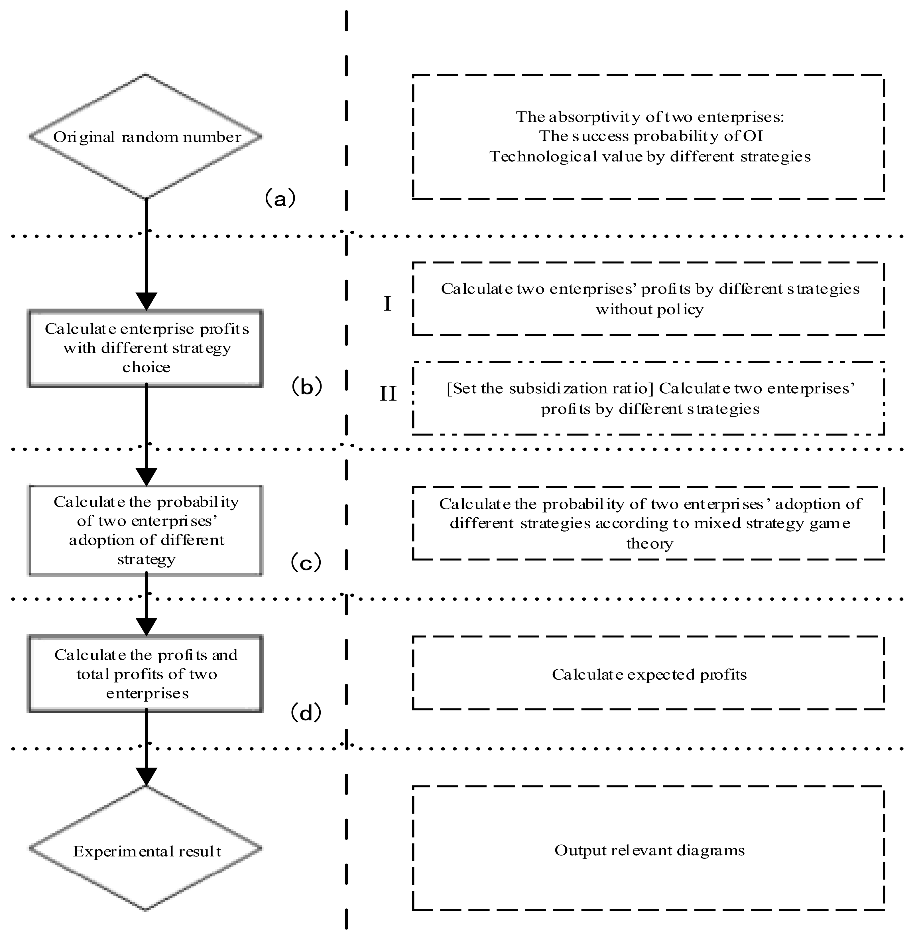
In order to further study the impact of R&D subsidies on the stability of cooperation within open innovation systems, we constructed a simulation framework using random numbers. This method reduces the subjective assumptions of the simulation process and makes the process more objective [59]. This modeling process consists of four steps: (a) using MATLAB method to randomly generate input parameters; (b) establishing a regulatory model to calculate the enterprises’ profits based on different strategy choices; (c) calculating the probability of the enterprises’ adoption of different strategy according to mixed strategy game theory; and (d) calculating the total profits of the two enterprises (Figure 3).

500 tests were performed using a simulation based on the above design process. To examine open innovation behavior under unregulated conditions, we built a review regression model based on trial results. Model 1 examines the impact of partner firms’ absorptive capacity on cooperation strategies and tests Proposition 1. Model 2 tests Proposition 2 by screening the test results for scenarios in which the absorptive capacity of both enterprises is greater than the sample mean. The model is set as follows:

• Model 1:$x={\beta }_1{\beta }^B+{\epsilon }_1$
• Model 2:$x={\beta }_2\overline{V_f^A}+{\epsilon }_2$

In these models, $x$ is the probability that Enterprise A adopts a positive cooperation strategy; ${\beta }^B$ is the absorptivity of Enterprise B; $\overline{V_f^A}$ is the future value outflow of the existing technologies when Enterprise A adopts a positive cooperation strategy; ${\beta }_i,i=1,2$ is the parameter to be estimated; and ${\epsilon }_i,i=1,2$ is residual error. The regression results are given in

Table 4. Examination and regression results.

	Model 1	Model 2
${\beta }^B$	−3.999 ***
$\overline{V_f^A}$		−0.027 ***

Note: *** p < 0.01.

:

Model 1 shows that the regression coefficient of the absorptive capacity of Enterprise B is negative when other factors are not considered, which means that the stronger the absorptive capacity of Enterprise B, the less likely Enterprise A is to adopt a negative cooperative strategy. This supports Proposition 1. Similarly, in Model 2, where both enterprises are engaging in positive cooperation, the regression coefficient of the outflow of future value is negative. This indicates that the larger the absorption capacity of both parties, the greater the outflow of existing technical value under the active cooperation strategy and the lower the probability that either enterprise will adopt a positive cooperation strategy. This supports Proposition 2.

In order to examine the impact of R&D subsidies on firm behavior, the results of tests under two simulation conditions (subsidy rates of 20% and 40%) were screened to provide two samples to test Propositions 3 and 4. The probability of positive cooperation strategies emerging under simulation conditions I and II are shown in

Table 5. Descriptive statistic results (the data meet the requirements of Proposition 3 in simulation II).

	No Subsidy	Subsidized by 20%	Subsidized by 40%
Mean	0.066	0.933	0.917
Median	0	1	1
Mode	0	1	1
Standard deviation	0.244	0.258	0.289

and

Table 6. Descriptive statistic results (the data meet the requirements of Proposition 4 in simulation II).

	No Subsidy	Subsidized by 20%	Subsidized by 40%
Mean	0.066	0.039	0.024
Median	0	0	0
Mode	0	0	0
Standard deviation	0.244	0.172	0.129

.

As shown in Table 6, when Proposition 3 is satisfied, R&D subsidy significantly increases the probability that an enterprise will adopt a positive cooperation strategy; however, the test results do not demonstrate the monotony described in Proposition 3. We believe this is due to normal error. Meanwhile, as R&D subsidy increases, the probability of adopting positive cooperation strategies is gradually reduced. This confirms Proposition 4.

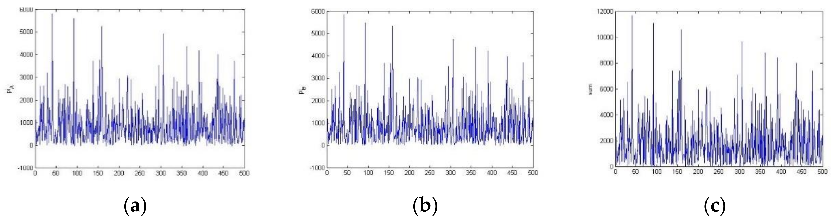
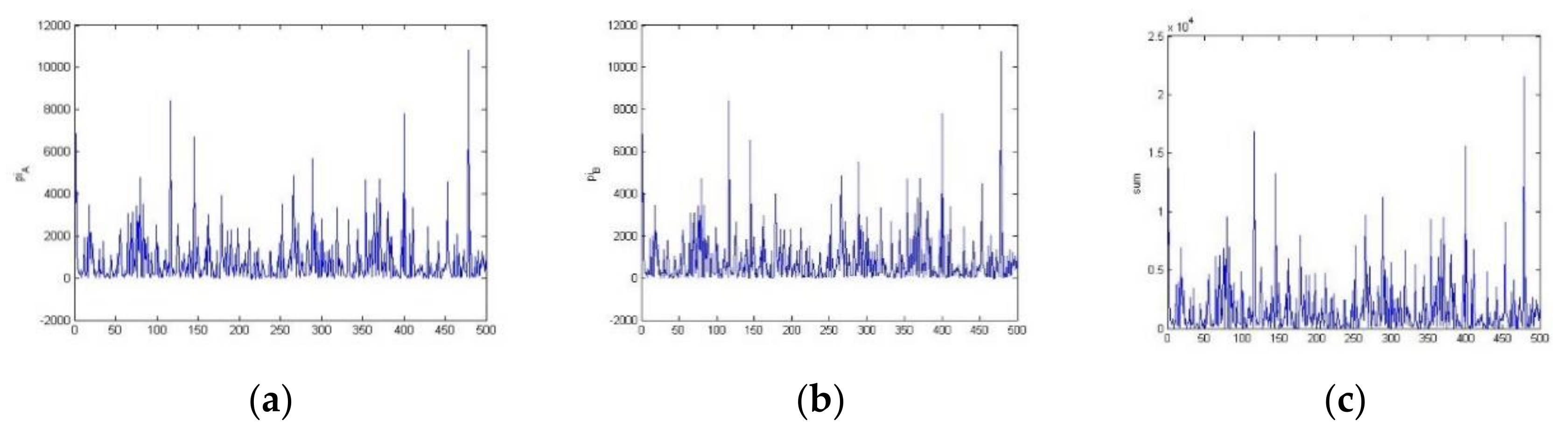
The simulation of the innovation outputs of Enterprise A and Enterprise B is shown in Figure 4.

Simulation I produces a random fluctuation of innovation. Only 14 trials (2.8%) resulted in both companies adopting positive cooperation strategies, while at least one company adopted a negative strategy in the remaining 486. This shows that in an unregulated environment, enterprises are much more likely to adopt a less active cooperation strategy; this is consistent with what is seen in empirical studies.

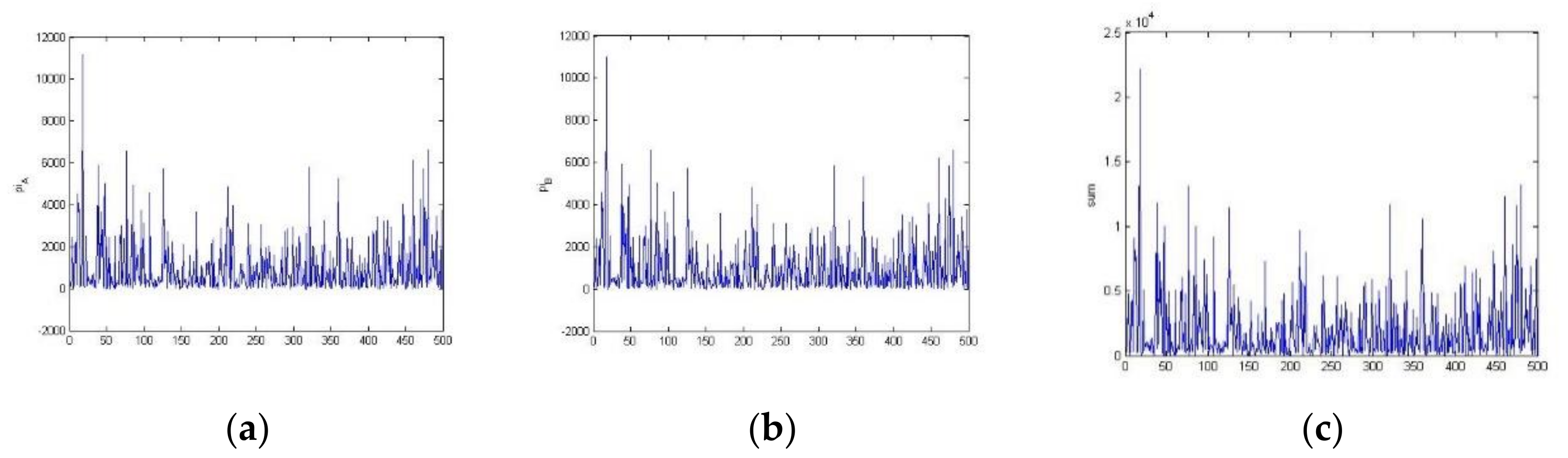
Figure 5 and Figure 6 show the outputs under different regulatory situations (subsidy rate 20% and 40%).

As shown in Figure 5 and Figure 6, both enterprises’ outputs fluctuate depending on policy subsidies. When the subsidy rate is 20%, there are only ten occasions (2%) in which both enterprises adopt a positive cooperation strategy. When the rate is 40%, there are only four occasions (0.8%). The randomness of output was further analyzed using a run test, the results of which are shown in

Table 7. Run test results.

Experiment Type	Statistics	p Value
No subsidies	1.97	0.049
Subsidized by 20%	−1.164	0.244
Subsidized by 40%	1.074	0.283

.

These results show that when the subsidy rate is 20%, output is generally lower that of firms receiving no subsidies; however, variance in output increases by 38.4%. At a funding rate of 40%, overall output increases, but variance also increases, in this case by 42.9%.

4. Conclusions

The scientific novelty of this research lies in expanding the theoretical understanding of the impact of macroeconomic policy on micro-enterprise behavior. Using game analysis, this paper examines how innovation policy can exert different effects on cooperation stability and innovation performance under different conditions defined by absorptive capacity, cooperation frequency, and technical value. Previous research has ignored the driving factors of cooperation behavior and technological innovation, and has lacked an in-depth analysis of how policy influences changes in subject behavior and other technological innovation system functions [33]. Game theory offers a better understanding of how innovative entrepreneurial behavior at the micro-level both drives and responds to innovation policies at the macro-level, rather than simply assuming that macro-level policies should or can drive micro-level behavior, as previously expected, Kivimaa and Kern [12] and Barykin et al. [60] suggest that decisions involving innovation are made based on the methodology and efficiency of possible forms of cooperation.

Our modeling indicates that in incidental innovation cooperation, enterprises are more willing to adopt active cooperation strategies when their partners have lower absorptive capacity. Only when the combined technological value of the partners meets a certain threshold is the probability of positive cooperative behavior improved; otherwise, non-positive cooperative behavior is encouraged. The performance of open innovation shows random fluctuation, and while R&D subsidies improve innovation performance, they also increase this randomness. The theoretical contribution of this research responds to the fact that the realization of open innovation requires in-depth study of different modes. The realization of OI in each given mode requires different situational conditions, and different research designs are required to adapt to the market power, technological value, and absorptive capacity of the partners. At the same time, different cooperation modes also require different support policies. The foundation of current energy industry policy is to promote sustainable development, and the core of sustainable development is continuous innovation and even subversive innovation. The renewable energy sector is characterized by continual technological advancement. Along with policies that stimulate market demand, renewable energy development requires policies that protect intellectual property and provide long-term R&D support. However, as this study shows, it is not enough for governments to provide R&D subsidies; more important is the promotion of integrity, activity, and interaction between innovation entities along the industrial chain. Specifically, R&D subsidies and policy should target barriers to open innovation in order to foster stable cooperation among actors and ensure the sustainable development of the open innovation system. On a broader level, we believe findings from this study have the potential to help society move towards more efficient management of knowledge production and diffusion to address the challenges of a range of industries, resulting in more sustainable development.

Although observations specific to the wind power industry underlie our simulations as presented in this paper, the findings are expected to apply to some degree to other sectors in which policy instruments are used to promote innovation. Further empirical studies are encouraged to test these findings in other sectors. Future work should also pursue the design of open innovation operating mechanisms within the framework of an innovation ecosystem to encourage positive cooperation and full integration of innovation resources and improve operation efficiency.

References

- Du, J.; Leten, B.; Vanhaverbeke, W. Managing open innovation projects with science-based and market-based partners. Res. Policy 2014, 43, 828–840. [Google Scholar] [CrossRef]
- Hajek, P.; Henriques, R.; Hajkova, V. Visualising components of regional innovation systems using self-organizing maps—Evidence from European regions. Technol. Forecast. Soc. Chang. 2014, 84, 197–214. [Google Scholar] [CrossRef]
- Von Krogh, G.; Netland, T.; Wörter, M. Winning with open process innovation. MIT Sloan Manag. Rev. 2018, 59, 53–56. [Google Scholar]
- Friesike, S.; Widenmayer, B.; Gassmann, O.; Schildhauer, T. Opening science: Towards an agenda of open science in academia and industry. J. Technol. Transf. 2015, 40, 581–601. [Google Scholar] [CrossRef] [Green Version]
- Keko, E.; Prevo, G.J.; Stremersch, S. The what, who and how of innovation generation. In Handbook of Research on New Product Development; Edward Elgar Publishing: Cheltenham, UK, 2018. [Google Scholar]
- Hirth, L.; Müller, S. System-friendly wind power: How advanced wind turbine design can increase the economic value of electricity generated through wind power. Energy Econ. 2016, 56, 51–63. [Google Scholar] [CrossRef]
- Tucci, C.L.; Chesbrough, H.; Piller, F.; West, J. When do firms undertake open, collaborative activities? Introduction to the special section on open innovation and open business models. Ind. Corp. Chang. 2016, 25, 283–288. [Google Scholar] [CrossRef]
- Gao, W.; Wu, C.; Qiao, G.; Wang, X. The Empirical Study on the Transmission Effect of R&D subsidy Policies in China’s Wind Power Industry. China Soft Sci. 2017, 11, 54–65. [Google Scholar]
- Chesbrough, H. The future of open innovation: The future of open innovation is more extensive, more collaborative, and more engaged with a wider variety of participants. Res.-Technol. Manag. 2017, 60, 35–38. [Google Scholar] [CrossRef]
- Hitchen, E.L.; Nylund, P.A.; Viardot, E. The effectiveness of open innovation: Do size and performance of open innovation groups matter? Int. J. Innov. Manag. 2017, 21, 1750025. [Google Scholar] [CrossRef]
- Vogelpohl, T.; Ohlhorst, D.; Bechberger, M.; Hirschl, B. German renewable energy policy: Independent pioneering versus creeping Europeanization? In A Guide to EU Renewable Energy Policy; Edward Elgar Publishing: Cheltenham, UK, 2017. [Google Scholar]
- Kivimaa, P.; Kern, F. Creative destruction or mere niche support? Innovation policy mixes for sustainability transitions. Res. Policy 2016, 45, 205–217. [Google Scholar] [CrossRef] [Green Version]
- Greenhalgh, C.; Rogers, M. The value of intellectual property rights to firms and society. Oxf. Rev. Econ. Policy. 2007, 23, 541–567. [Google Scholar] [CrossRef]
- Hall, B.; Helmers, C.; Rogers, M.; Sena, V. The choice between formal and informal intellectual property: A review. J. Econ. Lit. 2014, 52, 375–423. [Google Scholar] [CrossRef] [Green Version]
- West, J. How open is open enough? Melding proprietary and open source platform strategies. Res. Policy 2003, 32, 1259–1285. [Google Scholar] [CrossRef]
- Thomä, J.; Bizer, K. To protect or not to protect? Modes of appropriability in the small enterprise sector. Res. Policy 2013, 42, 35–49. [Google Scholar] [CrossRef]
- Hong, Y.; Li, Y. Research on the policy transmission mechanism of independent innovation. Stud. Sci. Sci. 2012, 3, 449–457. [Google Scholar]
- Georghiou, L.; Edler, J.; Uyarra, E.; Yeow, J. Policy instruments for public procurement of innovation: Choice, design and assessment. Technol. Forecast. Soc. Chang. 2014, 86, 1–12. [Google Scholar] [CrossRef]
- Nilsson, M.; Moodysson, J. Regional innovation policy and coordination: Illustrations from Southern Sweden. Sci. Public Policy 2015, 42, 147–161. [Google Scholar] [CrossRef]
- Bogers, M.; Chesbrough, H.; Moedas, C. Open innovation: Research, practices, and policies. Calif. Manag. Rev. 2018, 60, 5–16. [Google Scholar] [CrossRef]
- Liang, J.; Fiorino, D.J. The Implications of Policy Stability for Renewable Energy Innovation in the United States, 1974–2009. Policy Stud. J. 2013, 41, 97–118. [Google Scholar] [CrossRef]
- Kim, K.; Kim, Y. Role of policy in innovation and international trade of renewable energy technology: Empirical study of solar PV and wind power technology. Renew. Sustain. Energy Rev. 2015, 44, 717–727. [Google Scholar] [CrossRef]
- Costa, J.; Matias, J.C. Open innovation 4.0 as an enhancer of sustainable innovation ecosystems 0 as an enhancer of sustainable innovation ecosystems. Sustainability 2020, 12, 8112. [Google Scholar] [CrossRef]
- Verhees, B.; Raven, R.; Kern, F.; Smith, A. The role of policy in shielding, nurturing and enabling offshore wind in The Netherlands (1973–2013). Renew. Sustain. Energy Rev. 2015, 47, 816–829. [Google Scholar] [CrossRef] [Green Version]
- Barykin, S.Y.; Bochkarev, A.A.; Sergeev, S.M.; Baranova, T.A.; Mokhorov, D.A.; Kobicheva, A.M. A methodology of bringing perspective innovation products to market. Acad. Strateg. Manag. J. 2021, 20, 1–19. [Google Scholar]
- Del Río, P.; Mir-Artigues, P. Support for solar PV deployment in Spain: Some policy lessons. Renew. Sustain. Energy Rev. 2012, 16, 5557–5566. [Google Scholar] [CrossRef]
- Hoppmann, J.; Huenteler, J.; Girod, B. Compulsive policy-making—The evolution of the German feed-in tariff system for solar photovoltaic power. Res. Policy 2014, 43, 1422–1441. [Google Scholar] [CrossRef]
- Jacobsson, S.; Karltorp, K. Mechanisms blocking the dynamics of the European offshore wind energy innovation system–Challenges for policy intervention. Energy Policy 2013, 63, 1182–1195. [Google Scholar] [CrossRef]
- Dubina, I.; Carayannis, E.G. Potentials of game theory for analysis and improvement of innovation policy and practice in a dynamic socio-economic environment. J. Innov. Econ. Manag. 2015, 3, 165–183. [Google Scholar] [CrossRef]
- Longo, M.C.; Giaccone, S.C. Struggling with agency problems in open innovation ecosystem: Corporate policies in innovation hub. TQM J. 2017, 29, 881–898. [Google Scholar] [CrossRef]
- Bergek, A.; Hekkert, M.; Jacobsson, S.; Markard, J.; Sandén, B.; Truffer, B. Technological innovation systems in contexts: Conceptualizing contextual structures and interaction dynamics. Environ. Innov. Soc. Transit. 2015, 16, 51–64. [Google Scholar] [CrossRef] [Green Version]
- Valkokari, K.; Seppänen, M.; Mäntylä, M.; Jylhä-Ollila, S. Orchestrating innovation ecosystems: A qualitative analysis of ecosystem positioning strategies. Timreview 2017, 7, 12–24. [Google Scholar] [CrossRef]
- Kuhlmann, S.; Shapira, P.; Smits, R. Introduction. A systemic perspective: The innovation policy dance. In The Theory and Practice of Innovation Policy. An International Research Handbook; Edward Elgar: Cheltenham, UK, 2010; pp. 1–22. [Google Scholar]
- Lauber, V. Wind power policy in Germany and the UK: Different choices leading to divergent outcomes. In Learning from Wind Power; Palgrave Macmillan: London, UK, 2012; pp. 38–60. [Google Scholar]
- Wood, G.; Dow, S. What lessons have been learned in reforming the Renewables Obligation? An analysis of internal and external failures in UK renewable energy policy. Energy Policy. 2011, 39, 2228–2244. [Google Scholar] [CrossRef]
- Chen, J.; Sheng, Y. Multi case study on the incentive mechanism of innovation policy in the interest of stakeholders. Stud. Sci. Sci. 2013, 7, 1109–1120. [Google Scholar]
- Costa, J. Carrots or Sticks: Which Policies Matter the Most in Sustainable Resource Management? Resources. 2021, 10, 12. [Google Scholar] [CrossRef]
- Silva, P.C.; Klagge, B. The evolution of the wind industry and the rise of Chinese firms: From industrial policies to global innovation networks. Eur. Plan. Stud. 2013, 21, 1341–1356. [Google Scholar] [CrossRef]
- Ru, P.; Zhi, Q.; Zhang, F.; Zhong, X.; Li, J.; Su, J. Behind the development of technology: The transition of innovation modes in China’s wind turbine manufacturing industry. Energy Policy 2012, 43, 58–69. [Google Scholar] [CrossRef]
- Arora, A.; Ceccagnoli, M. Patent protection, complementary assets, and firms’ incentives for technology licensing. Manag. Sci. 2006, 52, 293–308. [Google Scholar] [CrossRef]
- Henkel, J.; Schöberl, S.; Alexy, O. The emergence of openness: How and why firms adopt selective revealing in open inno-vation. Res. Policy 2014, 43, 879–890. [Google Scholar] [CrossRef]
- Lyu, Y.B.; Lan, Q.; Han, S.J. Growth genes of the open innovation ecosystem: Multi-case study based on iOS, Android and Symbian. China Ind. Econ. 2015, 5, 148–160. [Google Scholar]
- Koszegi, B. Behavioral contract theory. J. Econ. Lit. 2014, 52, 1075–1118. [Google Scholar] [CrossRef] [Green Version]
- Zacharias, N.A.; Daldere, D.; Winter, C.G. Variety is the spice of life: How much partner alignment is preferable in open innovation activities to enhance firms’ adaptiveness and innovation success? Bus. Res. 2020, 117, 290–301. [Google Scholar] [CrossRef]
- Gilsing, V.; Nooteboom, B.; Vanhaverbeke, W.; Duysters, G.; Van Den Oord, A. Network embeddedness and the exploration of novel technologies: Technological distance, betweenness centrality and density. Res. Policy. 2008, 37, 1717–1731. [Google Scholar] [CrossRef]
- Todorova, G.; Durisin, B. Absorptive capacity: Valuing a reconceptualization. Acad. Manag. Rev. 2007, 32, 774–786. [Google Scholar] [CrossRef]
- Savin, I.; Egbetokun, A. Emergence of innovation networks from R&D cooperation with endogenous absorptive capacity. J. Econ. Dyn. Control 2016, 64, 82–103. [Google Scholar]
- Kim, C.Y.; Seo, E.H.; Booranabanyat, C.; Kim, K. Effects of Emerging-Economy Firms’ Knowledge Acquisition from an Advanced International Joint Venture Partner on Their Financial Performance Based on the Open Innovation Perspective. J. Open Innov. Technol. Mark. Complex. 2021, 7, 67. [Google Scholar] [CrossRef]
- West, J.; Bogers, M. Leveraging external sources of innovation: A review of research on open innovation. J Prod Innov Manag. 2014, 31, 814–831. [Google Scholar] [CrossRef]
- de Paulo, A.F.; Porto, G.S. Solar energy technologies and open innovation: A study based on bibliometric and social network analysis. Energy Policy. 2017, 108, 228–238. [Google Scholar] [CrossRef]
- Wang, X.; Zou, H.; Zheng, Y.; Jiang, Z. How will different types of industry policies and their mixes affect the innovation performance of wind power enterprises? Based on dual perspectives of regional innovation environment and enterprise ownership. J. Environ. Manag. 2019, 251, 109586. [Google Scholar] [CrossRef]
- Megginson, W.L.; Fotak, V. Government Equity Investments in Coronavirus Bailouts: Why, How, When? How When 2020. [CrossRef]
- Audretsch, D.B.; Link, A.N.; Scott, J.T. Public/private technology partnerships: Evaluating SBIR-supported research. In The Social Value of New Technology; Edward Elgar Publishing: Cheltenham, UK, 2019. [Google Scholar]
- Acemoglu, D.; Akcigit, U.; Alp, H.; Bloom, N.; Kerr, W. Innovation, reallocation, and growth. Am. Econ. Rev. 2018, 108, 3450–3491. [Google Scholar] [CrossRef] [Green Version]
- Zúñiga-Vicente, J.Á.; Alonso-Borrego, C.; Forcadell, F.J.; Galán, J.I. Assessing the effect of public subsidies on firm R&D in-vestment: A survey. J. Econ. Surv. 2014, 28, 36–67. [Google Scholar]
- Noked, N. Integrated tax policy approach to designing research & development tax benefits. Va. Tax Rev. 2014, 34, 109. [Google Scholar]
- Gambardella, A.; Panico, C. On the management of open innovation. Res. Policy 2014, 43, 903–913. [Google Scholar] [CrossRef]
- Diestre, L.; Rajagopalan, N. Are all ‘sharks’ dangerous? new biotechnology ventures and partner selection in R&D alliances. Strateg. Manag. J. 2012, 33, 1115–1134. [Google Scholar]
- Sabor, K.K.; Thiel, S. Adaptive random testing by static partitioning. In Proceedings of the 2015 IEEE/ACM 10th Interna-tional Workshop on Automation of Software Test, Florence, Italy, 23–24 May 2015; pp. 28–32. [Google Scholar]
- Barykin, S.Y.; Kapustina, I.V.; Valebnikova, O.A.; Valebnikova, N.V.; Kalinina, O.V.; Sergeev, S.M.; Camastral, M.; Putikhin, Y.; Volkova, L. Digital technologies for personnel management: Implications for open innovations. Acad. Strateg. Manag. J. 2021, 20, 1–14. [Google Scholar]
Figure 1.
Flow chart of wind power blade design.
Figure 2.
Operation process of OI.
Figure 3.
The experiment process and theory of innovation output.
Figure 4.
Innovative output in simulation I. (a) Innovative output of Enterprise A (mean value: 877.1; variance: 904). (b) Innovative output of Enterprise B (mean value: 877.7; variance: 900). (c) Total innovative output (mean value: 1755; variance: 1803).
Figure 5.
Innovative outputs in simulation II (subsidy rate 20%). (a) Innovative output of Enterprise A (mean value: 783.8; variance: 1188). (b) Innovative output of enterprise B (mean value: 784.2; variance: 1182). (c) Total innovative output (mean value: 1568; variance: 2369).
Figure 6.
Innovative output in simulation III (subsidization rate is 40%). (a) Innovative output of Enterprise A (mean value: 964.5; variance: 1288). (b) Innovative output of Enterprise B (mean value: 966.1; variance: 1288). (c) Total innovative output (mean value: 1930; variance: 2576).