Article

Optimal Load and Energy Management of Aircraft Microgrids Using Multi-Objective Model Predictive Control

1
Department of Electrical and Electronic Engineering, Faculty of Engineering, University of Nottingham, Nottingham NG8 1BB, UK
2
Computational Optimisation and Learning Lab, School of Computer Science, University of Nottingham, Nottingham NG8 1BB, UK
3
Centre for Research on Microgrids (CROM), AAU Energy, Aalborg University, 9220 Aalborg East, Denmark
*
Author to whom correspondence should be addressed.
Sustainability 2021, 13(24), 13907; https://0-doi-org.brum.beds.ac.uk/10.3390/su132413907
Submission received: 25 October 2021 / Revised: 1 December 2021 / Accepted: 12 December 2021 / Published: 16 December 2021

Abstract

:
Safety issues related to the electrification of more electric aircraft (MEA) need to be addressed because of the increasing complexity of aircraft electrical power systems and the growing number of safety-critical sub-systems that need to be powered. Managing the energy storage systems and the flexibility in the load-side plays an important role in preserving the system’s safety when facing an energy shortage. This paper presents a system-level centralized operation management strategy based on model predictive control (MPC) for MEA to schedule battery systems and exploit flexibility in the demand-side while satisfying time-varying operational requirements. The proposed online control strategy aims to maintain energy storage (ES) and prolong the battery life cycle, while minimizing load shedding, with fewer switching activities to improve devices lifetime and to avoid unnecessary transients. Using a mixed-integer linear programming (MILP) formulation, different objective functions are proposed to realize the control targets, with soft constraints improving the feasibility of the model. In addition, an evaluation framework is proposed to analyze the effects of various objective functions and the prediction horizon on system performance, which provides the designers and users of MEA and other complex systems with new insights into operation management problem formulation.

1. Introduction

Onboard power demands increase dramatically with the development of more electric aircraft (MEA) and the replacement of traditional hydraulics and pneumatics by electrical systems to achieve higher efficiency and less fuel burn [1]. Critical loads, which are responsible for flight safety, such as flight surface actuators and environmental control systems, must be powered in all flight scenarios regardless of high-power peaks or fault-causing emergencies. The energy storage system (ESS) has an important role in MEA, not only for supporting bus voltages, but also as a backup to deal with power shortages during faults occurring in generation or transmission systems, or high-power peaks. In addition, shedding of non-critical loads (e.g., passenger cabin lighting) is also used to reduce peak power usage, helping to maintain power for safety-critical loads [2]. Intelligently combining the load shedding with the ESS capabilities is essential for the safe onboard electrical power system (EPS) operation.
Due to the complexity of MEA optimal operation management and the importance of their safety and reliability resulting from an advanced operating strategy, considerable attention is being devoted to developing suitable models and algorithms. Finite state machines are adopted in [3,4,5] to model the onboard DC-based EPS of MEA as a set of states and transitions. In these studies, several sets of safety rules are defined to cope with different failure cases to ensure uninterrupted power supply to the high priority loads. However, this method relies on accurate measurements to change the operation state and it is hard to integrate multiple operating goals. In addition, setting optimal rules can be difficult for complex systems because of the large number of system states.
Heuristic and metaheuristic algorithms are also widely used to solve energy and load management problems for microgrids (MGs), such as fuzzy logic algorithm [6,7,8,9], genetic algorithms [10,11,12], particle swarm optimization [13,14,15], and evolutionary algorithms [16,17]. However, these approaches are not suitable for real-time application, since they might fall into the trap of suboptimal solutions and can still be computationally intensive. Neural networks, studied in [18,19], are fast but need training, hence are less capable of coping with unexpected situations, and it can be difficult to verify their reliability for aircraft usage.
Recently, model predictive control (MPC) has drawn the attention of the power system community for the control and operation management of MGs. MPC provides an optimal operating strategy based on predicted future system trajectories, thereby avoiding operating based on the worst-case scenarios with high costs. The inherent feedback mechanism of MPC stemming from its receding horizon mechanism makes the system more robust against uncertainty [20]. In [21,22], an MPC-based hierarchical control structure is applied for achieving economic efficiency in residential MGs. In [23,24], MPC supervisory control is used to compensate for the mismatch between the offline scheduling process and the real-time operation of a hybrid PV-wind-battery MG. In this research, system models are formulated as Mixed-Integer Linear Programming (MILP) problems. The MPC method is adopted for battery management in hybrid electric vehicles (HEV) in [25,26], in which the MPC controller attempts to minimize the vehicle equivalent fuel consumption and the battery capacity fade at the same time. To enhance the battery lifespan and power performance, references [27,28] propose an MPC approach to reduce the battery power variation and maintain supercapacitors’ SOC at their desired values. In [29], the battery capacity fading is described by an online least-squares identification method, and the degradation cost function is used in the MPC scheme to increase the battery lifetime. Since MPC has shown good performance for residential MGs and HEVs energy management, researchers have been exploring the possibility of its application in MEA EPS. In the application for MEA, on the one hand, the controller can cope with system future dynamics with limited uncertainty, benefiting from the intrinsic corrective characteristic of MPC due to the rolling horizon strategy. On the other hand, the system operational and time-coupling constraints can be integrated into the MPC model. In [30], a hierarchical MPC framework for a hybrid propulsion system is presented to minimize power generation costs and delivery losses. However, the possibility of load shedding and system failure is not considered. In [31], a rate-based MPC method is adopted for power-sharing between two generators that are driven by the same engine. The optimal energy management based on MPC by sharing power among different power sources for an onboard hybrid propulsion system is studied in [32]. In [33,34], MPC is used for both power scheduling and load shedding optimization to cope with scenarios with one generator and one transmission cable failure. In [35,36], targeting energy management, hierarchical MPC controllers are proposed to coordinate multi-timescale system dynamics of the onboard power system from vehicle level to component level, where graph theory is adopted to model the multi-physics behavior. However, in these papers, the MPC for battery management is not the focus and the control problem is formulated without much detail about, for example, how to cope with different control targets and increase algorithm feasibility, which has left considerable scope for further investigation and analysis here. Hence, this paper aims to address these issues in the proposed MPC strategy for MEA EPS.
In the aforementioned works of the MPC applications, the flexibility of the MPC design including the objective function formulation, prediction horizon length, and the weighting factors to prioritize different operating criteria and the related impacts to the system performance has been neglected by adopting empirical settings. Investigating how these degrees of freedom can affect the control system performance will help to better decide the settings of MPC to meet system requirements. This paper will contribute to this investigation by designing a system-level MPC-based operation management strategy for a MEA. The analysis in this study can be extended to other complex systems including storage systems and load management.
In the studied system, the MPC controller aims to keep the battery energy storage highly charged, with fewer power variations to prolong the battery life cycle, and to minimize load shedding, with fewer contactor switching. Organizing these operating criteria in the form of an appropriate objective function is essential for MPC optimization models. However, the flexibility in the formulation of the objective functions adds to the complexity of the design.
In this paper, to solve the multi-objective optimal operation management problem of the MEA EPS, an MPC-based operation management strategy is introduced aiming at intelligently managing the onboard energy storage systems and exploiting flexibility in the demand-side while satisfying time-varying operational requirements. Different objective functions are proposed with various cost function terms to reach the MEA operating goals, where each objective function can perform differently for each control target. To evaluate the designed control system performance, an evaluation index for each target is proposed to quantify system performance for overall flight stages. All objective functions are evaluated by the proposed indices with the prediction horizon changing from short to long; hence, the impact of various prediction horizons for each objective function can be compared. This evaluation procedure is conducted with the load profiles having different changing frequencies and variations so that the analysis can consider different load cases. Based on the proposed index for each target, a multi-objective evaluation index is also proposed as an overall performance criterion, by which the final selection of the objective function and the length of the prediction horizon can be performed.
In addition to analysis of the degrees of freedom in an MPC setting, this work also improves the feasibility of the MPC-based control strategy to adapt the controller to real-time operating conditions. On the one hand, soft constraints are introduced to cope with the non-accurate estimation of the battery SOC. The optimization problem to be solved by the control system is formulated as a MILP problem, which includes both objective functions and system constraints related to the system power flow, energy conversion, and connection constraints, benefitting from certainty for global optimal solutions [37]. As the system only operates normally when the MILP-MPC algorithm provides a feasible solution, the algorithm should tolerate bounds exceeding situations (i.e., SOC exceeds the target range). On the other hand, the real-time application requires that the sample time of the MPC can meet the possible computation time variations when dealing with different operating conditions. For each objective function, the worst-case values of the maximum computation time are recorded for various prediction horizon lengths. The sample time can be selected appropriately by considering the maximum computation time at the design stage, which guarantees that the MPC can be adopted for online optimization in real-time. Finally, a real-time test is conducted for the studied system, to verify the real-time application of the proposed MPC-based operation management strategy.
The rest of this paper is organized as follows: the MEA system under consideration is presented in Section 2 while the proposed MILP-MPC controller framework is introduced in Section 3. The system model with different objective functions is proposed in Section 4. In Section 5, the evaluation framework is set up, based on which, the performance for each objective function is evaluated with the changing prediction horizon for two different load profiles. The real-time analysis regarding the sample time selection is also presented in this section. The real-time experiment setup and the results are presented in Section 6. Finally, conclusions are drawn in Section 7.

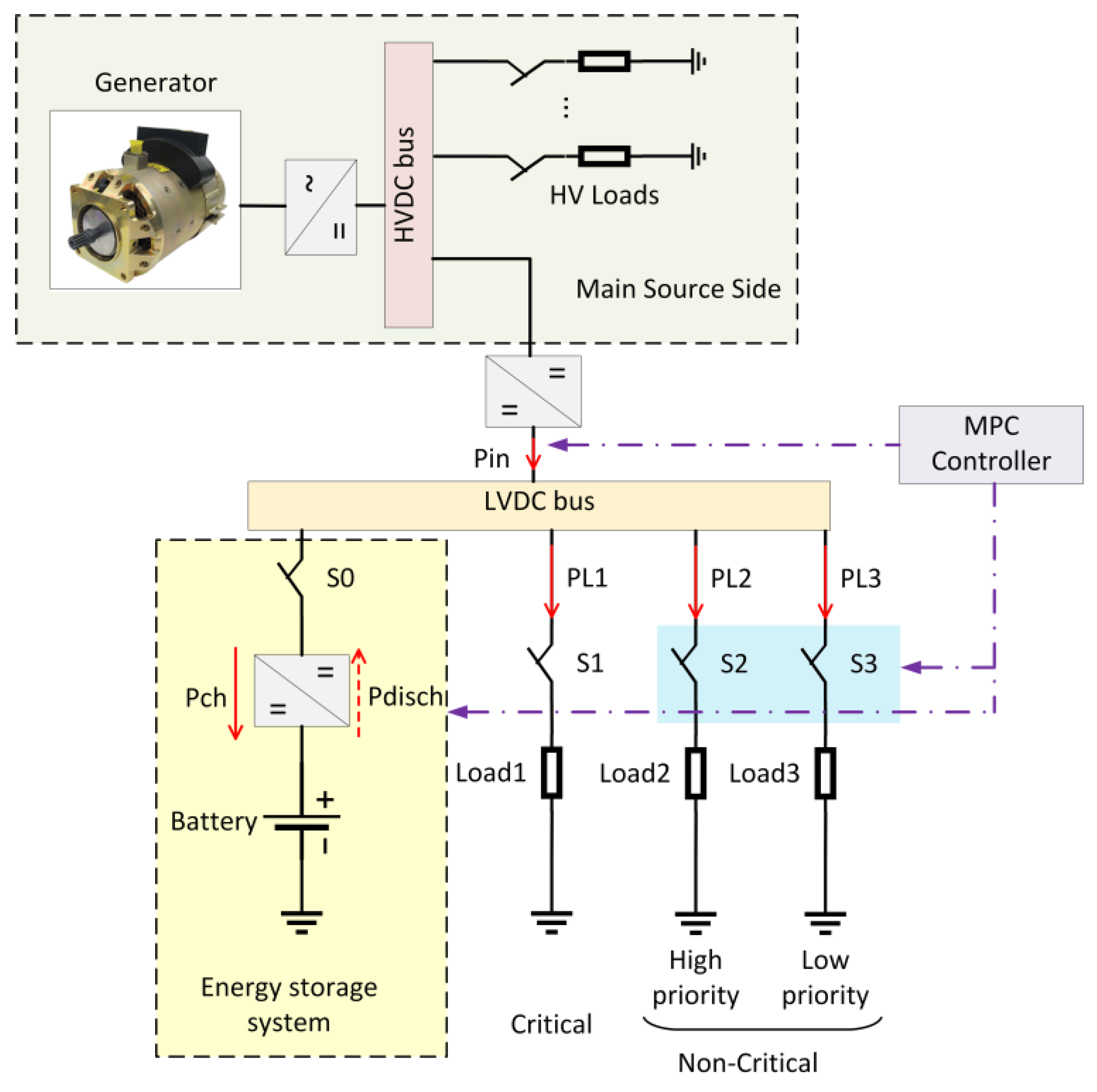
2. System Description

The EPS on the aircraft are normally symmetrically allocated for the left and right sides [38]. Figure 1 presents the architecture for one side of EPS studied in this work, and all the main symbols used in this paper are listed in Table 1. As can be seen in this figure, the EPS includes a main source (MS) consisting of one generator connected to an HV bus, an ESS, DC/DC power converters, and several loads. The MS powers the loads connected to a low voltage (LV) bus. In this system, the ES, which consists of one battery, one bidirectional DC/DC converter, and one contactor, is connected to the same LV bus, to both maintain the bus voltage and supply the loads when faults result in insufficient power available from the MS. It is worth mentioning that this paper focuses on the load and ES management for the LV bus as an example to study the objective formulizations. However, the proposed method can be applied to the HV side or other EPS architectures [39].
The MEA loads can be classified into critical and non-critical loads. Critical loads link with flight safety status and avionics systems, such as environment control system and flight control system, etc. The non-critical loads are the other classes of loads that provide a comfortable environment for passengers and some of them are more essential, which are assigned with a higher priority. For example, the in-flight entertainment and galley services are considered as a lower priority load compared to other non-critical loads such as water and waste systems [40,41]. Therefore, in this study, three types of loads are considered, namely, critical loads (Load1) which must be supplied under all circumstances, high priority loads (Load2), which can be shed but should not where possible, and low priority loads (Load3), which should be shed in preference to high priority loads when load shedding is needed.
The control system is responsible for optimizing the control commands related to the MS (Pin) and ES (Pbatt) as well as determining the connection/disconnection status of non-critical loads (SLi) to guarantee power balance in the system while following operational goals. To do so, the power from the MS and the battery should equal the required power by the connected critical and non-critical loads, as shown below. In Equation (1), the binary decision variable S L i ( k ) indicates that the entire load will be supplied/shed by connecting/disconnecting the associated switch and there is no partial shedding. However, based on the load characteristics, it is straightforward to modify the model to shed part of the load if required.
P i n ( k ) P b a t t ( k ) i S L i ( k ) P L i s h e d ( k ) j P L j n o n s h e d ( k ) = 0
P b a t t ( k ) = P c h ( k ) P d i s c h ( k )
Equation (2) shows the battery power being equal to Pch(k) and Pdisch(k) during charging and discharging time, respectively. The charging/discharging power of the battery is the control command that needs to be determined by the EPS control system by directly adjusting the Pin as load power changes. The SOC of the battery as the system state variable is evaluated using the discrete dynamic equation in (3), which is essential for predicting the future status of the ESS.
S O C ( k + 1 ) = S O C ( k ) + T s · η c h · P c h ( k ) B c a p T s · P d i s c h ( k ) η d i s c h · B c a p
According to (1)–(3), the system model includes both continuous variables related to the power from the MS and the ESS as well as binary variables representing the connection/disconnection status of the noncritical loads. In addition, to avoid simultaneous charging/discharging of the battery, additional binary variables are introduced to show the charge/discharge status of the battery at each stage, which are formulized in (18)–(20) in Section 4.2 as charging/discharging mode constraints. The system dynamics introduced above together with operation limitations over the prediction horizon are considered as constraints in an MPC-based controller, which is presented in detail in Section 4. The core of the MPC strategy is a model of the system under control to predict the evolution of system output over the desired horizon. Thus, the system model introduced in this section is repeatedly updated based on the most recent information obtained from the system. In addition, a prediction of the system load over the prediction horizon is required.
The MEA load can potentially be predicted by online machine learning-based methods combining the adjustment of the flight stages, height, and historical data [24,42], which is out of the scope of this study. In this paper, the sampled load profile is used for prediction without adjustment for real-time flight power changes, and the deviations between the predicted load and the real values are neglected to simplify the analysis.

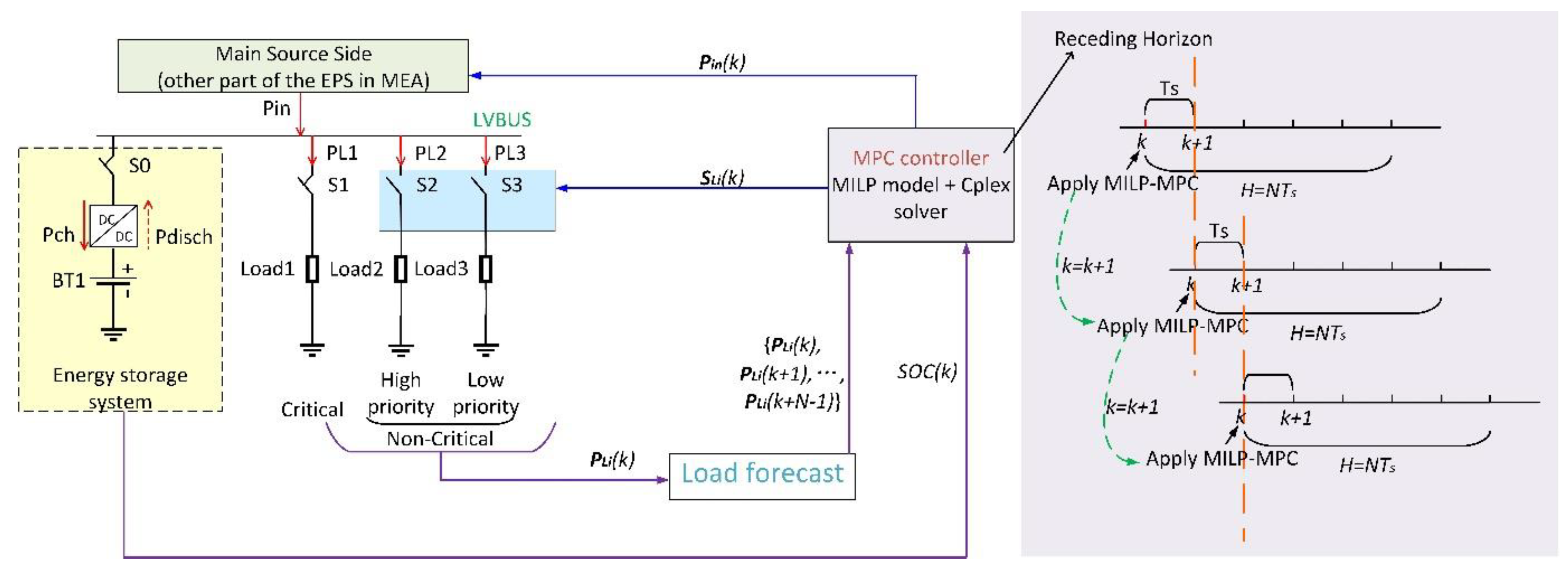
3. MILP-MPC Controller Framework

The proposed MPC-based control architecture is represented in Figure 2. This paper concentrates on the system-level MPC controller, with a slow time scale in the order of 1 min to optimize the long-term performance of the system. As can be seen in Figure 2, the controller received the updated information of the system at the beginning of each control cycle defined by the desired sampling time. This information includes the updated network constraints, battery status, and the prediction of the load demands and associated priorities.
The control problem of the target MEA is formulated as a dynamic MILP optimization problem, and the CPLEX solver [43] is used to solve the problem at each time step, guaranteeing to find an optimal solution for each time step. The MS-ES-L system is modeled as a discrete-time dynamic system with sampling time Ts as introduced in the previous section. The MILP-MPC controller framework is structured as follows.

MILP-MPC Framework

As illustrated in Figure 2, at each time step k, k = 0, 1, …, N − 1, an online optimization problem is solved over the finite prediction horizon H. The prediction horizon indicates the time looking ahead in the future to evaluate the cost function subject to several technical and operational constraints, which can be calculated as H = NTs [44]. The MPC works based on a receding horizon scheme presented in Figure 2. At each time step k, the MPC controller receives the updated status of the system and finds the solution of a finite horizon optimization problem. The result is an optimal control sequence over the optimization horizon. However, only the first sample of the optimal control sequence is applied to the system, and the control problem is shifted to the next time step k + 1 as shown in Figure 2. The MPC control procedure is explained in detail in the following Algorithm 1. The controller aims to keep the battery energy storage highly charged, with fewer power variations to prolong the battery life cycle, and to minimize load shedding, with fewer contactor switching that need to be appropriately modeled in the MPC optimization problem. The optimization problem including these operating criteria and system constraints is introduced in the next section.
Algorithm 1. MILP-MPC controller.
(1)
Update system state at time step k
(a)
Initialize the model with the measured/estimated state of the components, e.g., SOC(k), load power measurement PLi(k)
(b)
Predict load demands over the prediction horizon H at each future sampling time Ts,, e.g., PLi(k), PLi(k + 1), …, PLi(k + N − 1)
(2)
Perform optimization: the high-level controller computes the optimal input sequence for the prediction horizon H, based on the updated system status and the predictions of the future system behavior. The optimal input sequence includes the decision of load shedding or not (SLi, k = 0, 1, …, N − 1, H = NTs) and the input power reference on the MS-side Pin (k = 0, 1, …, N, H = NTs). The optimization problem is solved using the CPLEX solver.
(3)
Apply the first sample of the optimal control sequence.
(4)
Set k = k + 1, go to step 1, and repeat the process with the new state.

4. Formulation of Objectives and Constraints in MPC

The MEA system control problem can be mathematically modeled using a set of technical and operational constraints and objective functions. In this section, three different objective functions are proposed for multiple control targets, and the system constraints are introduced.

4.1. Designing the Objective Functions

There are several control targets followed by the MEA system under study. Firstly, the controller needs to minimize the total time for which loads are shed while maximizing the time duration for which the energy stored in the battery is kept within the target range (SOC(k) [LO, HI]). In addition, it needs to be ensured that the high priority loads are less shed than the low priority loads. Regarding the load management, instead of shedding/connecting loads continually, it is preferable to keep the contactors’ switching activity as low as possible to prolong the components lifetime, and to avoid the transients and instabilities in the system, even though this may potentially increase the total time for which loads are disconnected. Moreover, the battery is preferred to be charged/discharged smoothly rather than constantly changing the status between charging and discharging modes to improve the life span of the battery [45]. Apart from load shedding targets, the battery management-related goals could be formulated with different cost functions as well as different weighting factors for battery charging/discharging power, maintaining battery SOC, and minimizing battery power variation. The following three objective functions are therefore proposed to formulate the desired operating criteria and to analyze the effects of different cost functions on the system performance.

4.1.1. The First Proposed Objective Function (Obj1)

Obj1 in (4) denotes the first objective function combining the cost functions in (5)–(9) for each target by different weighting factors w S , w δ , w P c h , w P d i s c h , and w Δ . Cost function (5) indicates minimizing the total load shedding time by penalizing the shedding of loads with the load priorities. The change in load connections (connected/disconnected) for each time interval is minimized in (6). Since the energy stored in the battery can be calculated from the net power flowing to the battery, the cost function (7) and (8) can lead to maximizing the energy stored by penalizing the discharging and rewarding charging of the battery: the cost function in (7) encourages the system to charge the battery with as much power as is available, up to the rated value, while the cost function in (8) encourages the system to avoid battery discharging by minimizing the discharging power for every time interval. The charging speed of the battery can be changed by adopting different weighting factors for (7) and (8). For example, when w P c h > w S , the system will allow more load shedding to use power from the MS to charge the battery. When w P d i s c h w S w P c h , the system will shed loads when the battery is needed, but the charging will be slow as the MS priority is to supply loads rather than charging the battery.
O b j 1 = w S J S L i + w δ J δ L i + w P c h J P c h + w P d i s c h J P d i s c h + w Δ J Δ
where
J S L i = k = 0 N 1 i = 1 N L i γ L i ( 1 S L i ( k ) ) / N i = 1 N L i γ L i
J δ L i = k = 0 N 1 i = 1 N L i | S L i ( k + 1 ) S L i ( k ) | / N · N L i
J P c h = k = 0 N 1 ( P c h max P c h ( k ) ) / N P c h max
J P d i s c h = k = 0 N 1 ( P d i s c h ( k ) ) / N P d i s c h max
J Δ = k = 0 N 1 ( ε ( k ) + ϑ ( k ) ) / N
For battery management, the battery SOC is preferred to be kept in a target range (LO, HI) that can be modeled as a constraint. However, when there is a deviation between the predicted load and the realized load, the battery SOC might be temporarily out of the target range, which would prevent the solver from finding a feasible solution. Hence, rather than enforcing this requirement as a hard constraint, two slack variables ( ε ( k ) and ϑ ( k ) ) are introduced to penalize the deviation of the battery SOC from the target’s lower and upper bounds in the objective function as presented in (9). In this way, it is trying to keep the SOC within the target range or minimize the deviations. These variables are explained further in Section 4.2 below.

4.1.2. The Second Proposed Objective Function (Obj2)

Adding the cumulative battery SOC to the objective function will increase the average energy stored in the battery. Equation (8) represents a normalized cost function to increase the battery SOC to be as close as possible to the upper bound. Hence, Obj2 in (10) is formed by adding the battery SOC cost function to Obj1 in (4), with its weighting factor w S O C . Compared to the cost for charging/discharging power in (7) and (8), including SOC in the cost function will directly control SOC to maintain the desired reference value, which can be adjusted according to the applications. In this work, the desired reference value is set to be HI. Moreover, the charging will speed up more when longer prediction horizons are selected, as the SOC is a time-accumulated value, reflecting the accumulated charge for the whole prediction horizon.
O b j 2 = w δ J δ L i + w S J S L i + w S O C J S O C + w P c h J P c h + w P d i s c h J P d i s c h + w Δ J Δ
where
J S O C = k = 0 N 1 | H I S O C ( k + 1 ) | / ( N · H I )

4.1.3. The Third Proposed Objective Function (Obj3)

The aforementioned objective functions control the energy stored in the battery. However, proposing a cost function to prolong the battery life is also important for aircraft EPS for longer-term safe flights, for example, reducing the battery charging/discharging current variations and reducing charging/discharging operations [18]. In this work, it is assumed that the battery voltage has small deviations, so that reducing the battery charging/discharging current variations is equivalent to reducing the charging/discharging power variations. This also reduces the charging/discharging operations to reduce the charging cycle, which also benefits the battery lifetime. The cost for minimizing the battery charging/discharging power change J P b a t t is formulated by adding this prolonging battery lifetime cost to (13), where P b a t t ( k ) = P c h ( k ) P d i s c h ( k ) presents the battery net power. Obj3 represented in (12) is formulated by adding this prolonging battery lifetime cost to Obj2 in (10) with the weighting factor w P b a t t .
O b j 3 = w δ J δ L i + w S J S L i + w S O C J S O C + w P c h J P c h + w P d i s c h J P d i s c h + w P b a t t J P b a t t + w Δ J Δ
where
J P b a t t = k = 0 N 1 | P b a t t ( k + 1 ) P b a t t ( k ) | / N ( P c h max + P d i s c h max )

4.2. System Constraints

(1)
Power balance constraints
For the LV bus, the sum of power flowing into/out of it equals zero (Kirchhoff’s Current Law for a given voltage), assuming no losses within the bus itself. Hence, for the system presented in Figure 1, the power from the MS and the battery equals that required by the connected critical and non-critical loads, which can be formulated as (1) and (2), which is mentioned in Section 2.
(2)
Storage dynamics
The battery SOC can be calculated from the charging/discharging power over time using (3) presented in Section 2 [32].
(3)
Hard and soft constraints of SOC
Battery S O C [ 0 , 1 ] , where SOC = 1 indicates a fully charged battery, while SOC = 0 corresponds to a depleted battery. In the aircraft, SOC is preferred to be kept within a target range [LO, HI]. Therefore, upper and lower bounds are defined in (14), where LO = 0.3, HI = 0.9 is selected in this case, which could be presented as hard constraints for the optimization.
0.3 S O C ( k ) 0.9
However, the hard constraints (14) increase the sensitivity of the algorithm to the power fluctuations. Because SOC is related to the stored or released energy, which is influenced by the power fluctuations, it is necessary to allow SOC to vary slightly outside of this range in real situations, due to unpredicted power consumption variations. In this case, the hard constraints (14) would prevent finding a feasible solution. Therefore, soft constraints in (15)–(17) are proposed in our model to improve the feasibility of the solution strategy of the MILP-MPC algorithm. Variables ε(k) and ϑ(k) are introduced to relax the hard upper and lower bounds in (14). The maximum allowed deviation for both bounds is 0.1 in this case. By adding two large weight factors to ε(k) and ϑ(k) in the cost function as presented in Obj1 (4) and (9), SOC will usually be kept within the target range [0.3, 0.9], while allowing some tiny deviations when necessary.
0.3 ε ( k ) S O C ( k ) 0.9 + ϑ ( k )
0 ε ( k ) 0.1
0 ϑ ( k ) 0.1
(4)
Charging/discharging mode constraints
The battery can be either charged or discharged by the system. Therefore, two binary indicators are introduced to represent different modes in (18), (19), and (20), allowing the modes to be treated differently.
ζ c h ( k ) + ζ d i s c h ( k ) = 1 ,   ζ c h ( k ) ,   ζ d i s c h ( k ) { 0 , 1 }
0 P c h ( k ) ζ c h ( k ) · P c h max
0 P d i s c h ( k ) ζ d i s c h ( k ) · P d i s c h max
(5)
Bounds of input power from the MS-side
The input power from the MS-side is limited by the maximum power that can be transferred by the DC/DC converters, and these input power bounds are presented in (21)
0 P i n ( k ) P i n max

5. Evaluation for Various Objectives

The objective functions designed in Section 4 lead to different control problems and consequently different operating strategies for the MS-ES-L system, which are also impacted by the prediction horizon and the load profile. To compare the differences caused by these factors, an evaluation framework is proposed in this section to quantify the control results for all flight stages. The overall flight time is T = M·Ts, where M is the total number of time intervals. Moreover, to verify that the proposed method is suitable for real-time applications, the computation time for the MILP-MPC controller should be less than the sample time Ts. As the computation time can be impacted by the objective function formulation, prediction horizon, and load samples, the impact of these factors on the computation time is also studied in this section.

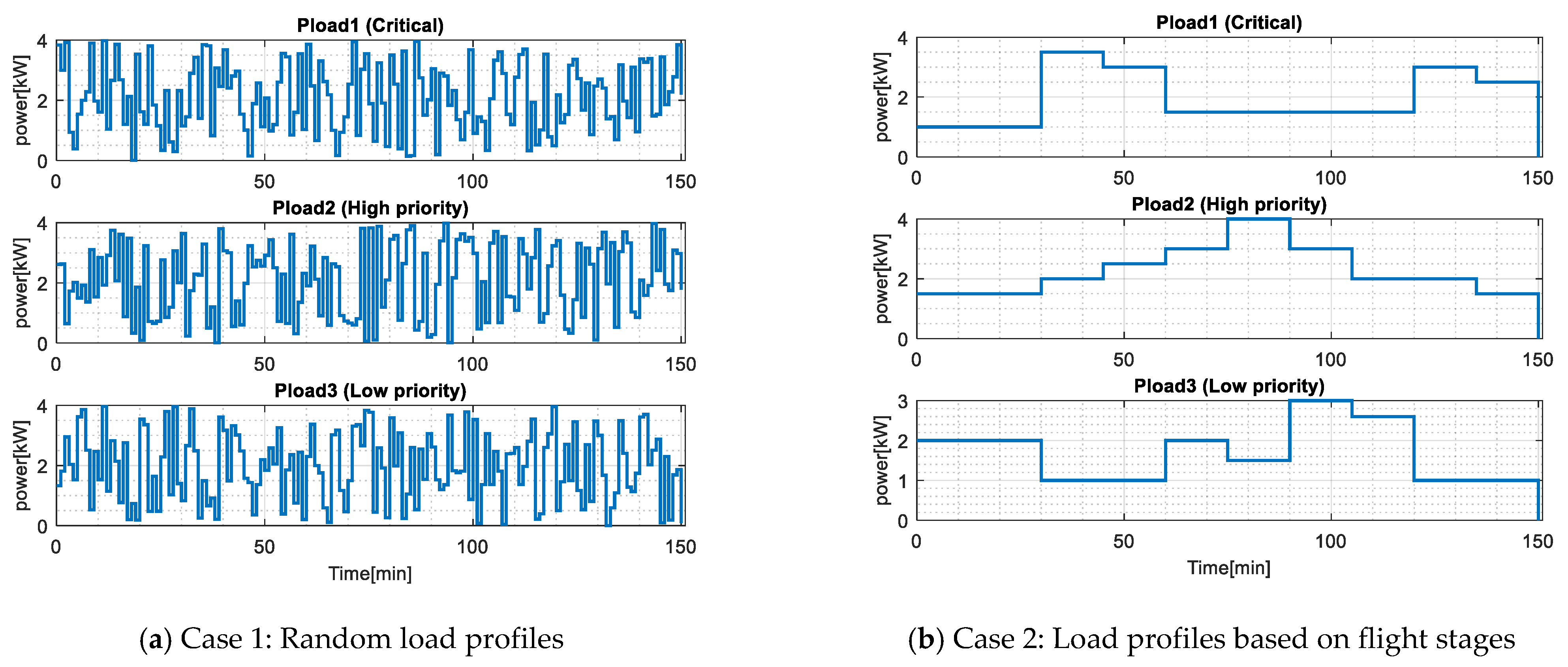
5.1. Model Parameters

The model parameters including the MS-ES-L system component parameters are listed in Table 2, and the weighting factors are listed in Table 3. These weighting factors are selected by the method proposed in [46]. The MILP-MPC controller sample time Ts is selected as 1 min, the verification for the sample time selection will be demonstrated in Section 5.3. The total flight time is 150 min.
For evaluating the load profile impacts on the results, two types of load profiles are used. In Figure 3a, a randomly changing load profile is considered, while Figure 3b demonstrates the load profiles based on different flight stages. The flight stages include ground (pre-departure and taxiing-out), takeoff, climb, cruise, descent, landing, and taxiing-in. Each load system requires a different amount of power at each flight stage. For example, the cabin power demand reaches the highest level at the cruise stage, which can be several times larger than the power demand at other stages. In addition, the power demand of the environment control system increases dramatically as soon as the aircraft takes off and keeps almost the same value for the following stages, while the landing gear only requires power during ground, takeoff, landing, and taxiing-in stages [47,48]. Therefore, compared to the load profiles in Figure 3a changing every minute, the profiles in Figure 3b change much slower where each load level lasts at least for 15 min. However, an average load power of 2 kW can be seen in both cases.

5.2. Evaluation Indices

In the following subsections, eight evaluation indices are proposed. The control results are evaluated by each of the proposed indices for both load scenarios when objectives Obj1–Obj3 are adopted for prediction horizons H varying from 1Ts to 30Ts (N = 1, 2, …, 30). Each index represents the corresponding quantified performance, and lower values indicate better performance.

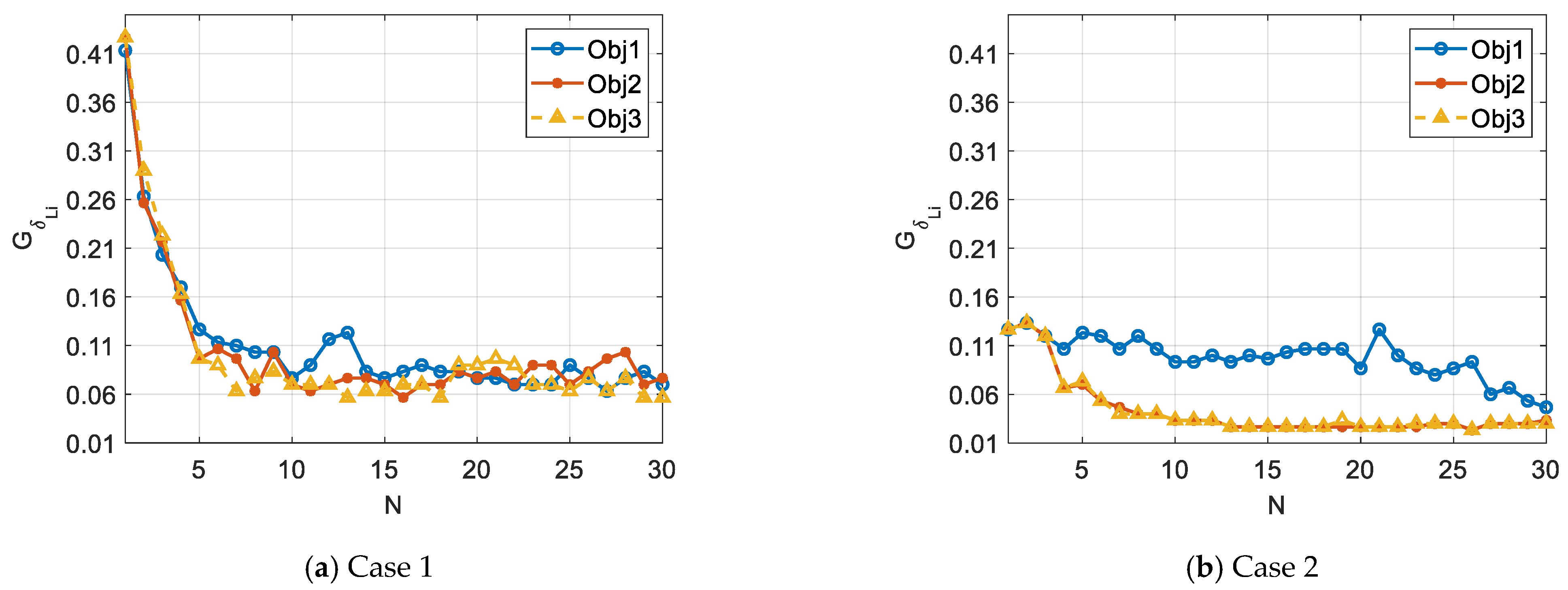
5.2.1. Load Shedding Index

The normalized load shedding index quantifies the ratio of shed loads throughout the whole flight time T = 150 min, as shown in (22).
G S L i = k = 0 M 1 i = 1 N L i [ γ L i ( 1 S L i ( k ) ) ] / ( M · i = 1 N L i ( γ L i ) )
In Figure 4, the load shedding index values are compared when adopting different prediction horizons and objective functions, with case 1 and case 2 showing the results for adopting different load profiles. For both load cases, the Obj2–3 have similar changes: when the prediction horizon is short, load shedding remains lower than for Obj1, while the load shedding increases quickly as the prediction horizon becomes longer, causing Obj2–3 to have more load shedding than Obj1 with long prediction horizons. Although the load shedding for Obj1 also has an incrementally increasing tendency when N increases for the second load case, the growth rate is much slower compared to Obj2–3. This difference between Obj1 and Obj2–3 is caused by the cost function JSOC-more loads are shed to speed up the SOC that accumulates when N increases.
Comparing Obj2 and Obj3, when the loads frequently vary, as presented in case 1, the load shedding for Obj3 increases at a higher rate than Obj2, while Obj3 has less load shedding than Obj2 when N ≤ 6. This is caused by the cost function JPbatt in Obj3. By changing the load shedding scheduling and adjusting the input power from MS, the battery can be charged/discharged smoothly. Combining with JSOC, more load shedding will be conducted as N increases so that the system keeps charging the battery with fewer power fluctuations. When the load varies less, and slowly, as load profiles in case 2, the load shedding curves for Obj2 and Obj3 are mostly overlapped, because the stable load profile lacks the scheduling possibilities while the WF for JPbatt is small; hence, JSOC dominates JPbatt in this case. Comparing the results for N = 9 in Figure 4, there is a sharp rise in the index value at N = 10, which indicates that the shedding of high-priority loads is increased.
In summary, Obj1 has better performance in load shedding compared to Obj2–3 on average. However, when the selected prediction horizon is not too long, e.g., N ≤ 9 in our case, the Obj2–3 can have better load shedding performance.

5.2.2. Contactor Status Change Index

The average number of connection status changes for each contactor in the whole period is presented in (23), where NLi indicates the total number of non-critical sheddable loads.
G δ L i = k = 0 M 1 i = 1 N L i | S L i ( k + 1 ) S L i ( k ) | / ( M · N L i )
These index values are compared in Figure 5 when adopting different prediction horizons and objective functions, with case 1 and case 2 showing the results for different load profiles. In general, the change in contactor status is reduced as N increases in both cases for Obj1–Obj3, while the curve for Obj1 in case 2 fluctuates the most. In both load cases, the contactor change values for Obj2–3 decrease very quickly when N < 10 and then keep a low level when the prediction horizon is longer. Moreover, when N is in this range, compared with the results for load shedding in Figure 4, Obj2–3 also has good performance for the load shedding index. This also benefits from the inclusion of JSOC, as it takes results of power integration over time into consideration within the prediction horizon.
It can be concluded that Obj2 and 3 perform better than Obj1 for maintaining the contactor status in different load cases. Moreover, for the contactor status change index, a very long prediction horizon is unnecessary for Obj2–3, saving computation time while still achieving good results.

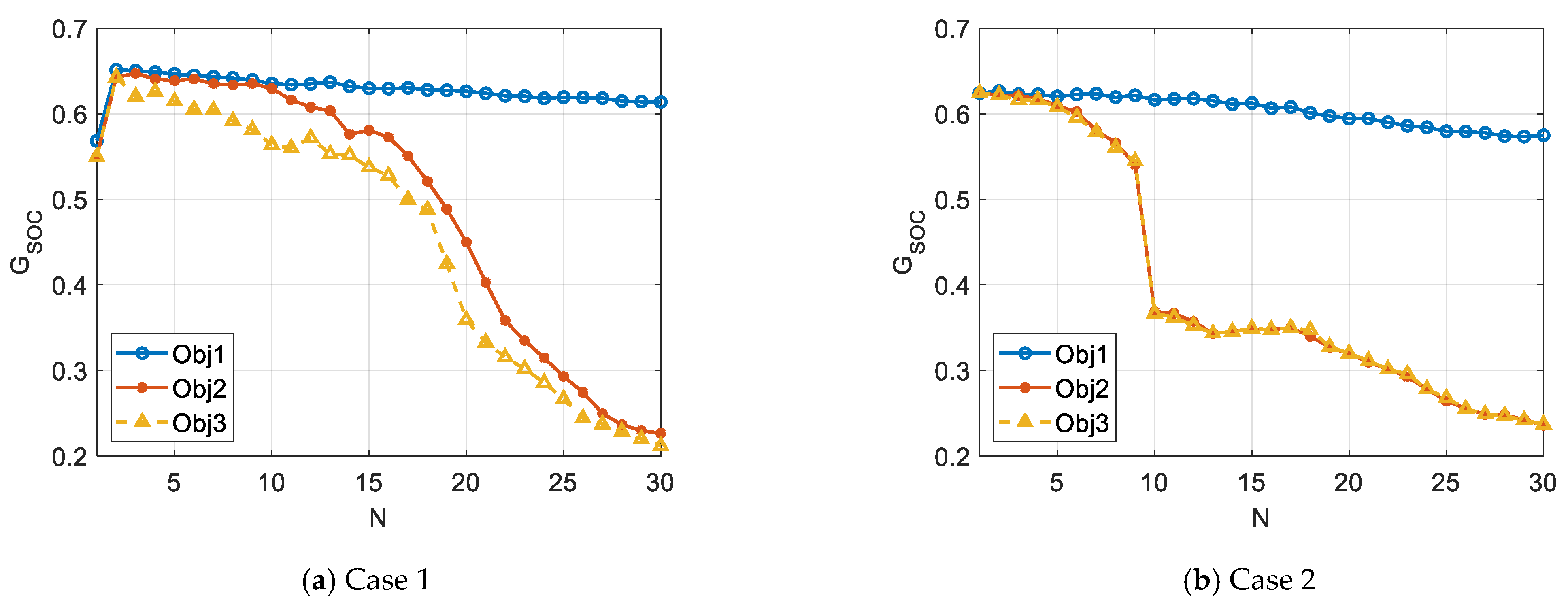
5.2.3. Battery Energy Storage Level Index

In aircraft applications, it is preferable to keep the battery highly charged to cope with emergency cases and unforeseen situations. Hence, when designing the optimization algorithms, the objective functions are designed to maximize the average energy stored in the battery. The index (24) is proposed to evaluate the average level of the energy stored during the studied scenarios.
G S O C = k = 0 M 1 | 0.9 S O C ( k ) | / ( M · 0.9 )
Figure 6 shows the comparison of the GSOC index values with different prediction horizons and objective functions, with case 1 and case 2 showing the results for adopting different load profiles. In general, the energy storage level index value is reduced as N increases in both cases for Obj1–Obj3, while for the load case 1, the index values for MILP (N = 1) are less than the ones for MILP-MPC (N ≥ 2) when N ≤ 12 for Obj3, N ≤ 16 for Obj2, and N ≤ 30 for Obj1. When N = 1, the contactor status changes will not impact the optimization results for each time step. Combined with the frequently varying loads, the SOC is therefore improved by shedding/connecting loads with high power demands continuously. However, when N = 2, the number of contactor status changes is much reduced (the index value is reduced by 1.3) compared to the value when N = 1. In the meantime, the battery will be used for supporting loads even the loads’ demands could be high, which slows down the SOC accumulation.
Comparing the SOC changing rate for Obj1–3 with the MILP-MPC method, for both load cases, Obj2 and 3 improve SOC level at a higher rate than Obj1 when N increases, since both Obj2 and Obj3 benefit from the cost function JSOC to speed up the energy storage in the long term. For load case 1, Obj3 speeds up the SOC accumulation with a higher rate than Obj2, as the cost function JPbatt in Obj3 tends to keep the battery charging with few power fluctuations.
This suggests that Obj3 has the best performance for the battery storage level index. When adopting Obj3, the prediction horizon does not necessarily need to be selected too long, as it charges the battery much faster than Obj1.

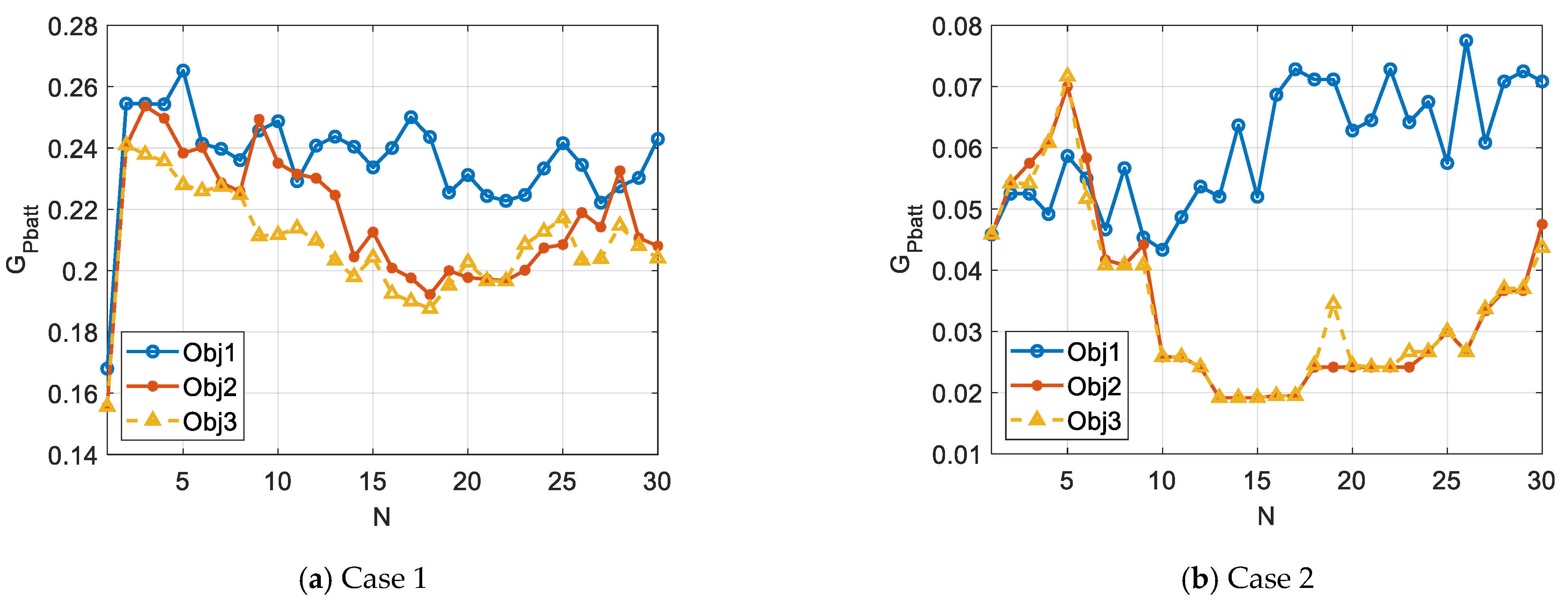
5.2.4. Battery Power Change Index

The battery life will be shortened when the battery power is frequently changed [18]. The index (25) is therefore proposed to calculate the total battery power change for all flight stages.
G P b a t t = k = 0 M 1 | P b a t t ( k + 1 ) P b a t t ( k ) | / M ( P c h max + P d i s c h max )
Figure 7 presents the comparison of the battery power change index values with different prediction horizons and objective functions, with case 1 and case 2 showing the results for adopting different load profiles. In both load cases, for each N, Obj3 usually has a better performance compared to Obj1, because Obj1 does not contain the cost function JPbatt to minimize the power change. However, as Obj2 has the cost function JSOC in common with Obj3 with relatively high WF, the index value curve of Obj2 has similar trends as Obj3—the value is reduced to the minimum value and then slightly rises with variations when N increases from 2 to 30. Because the load shedding and the reduction in the load on/off changes can avoid the battery changing between the charging and discharging modes, Obj2 and Obj3 perform similarly in these indices. By adding the cost function JPbatt in Obj3, the charging power can be smoothed whenever it is possible. On the other hand, when N increases (N > 20) to keep accumulating SOC, more power will be injected into the battery, thereby increasing the battery charging power variation. Moreover, JPbatt and JSOC can impact the results for load shedding and the contactor status changes, which results in the battery power change fluctuations, as can be seen in Figure 7.
Based on this comparison, Obj3 has the best performance for the index of battery power change, which also indicates that this objective function is preferred when battery life is important.

5.2.5. SOC Target Range Index

Since the soft constraints of SOC are introduced to improve the feasibility of the solution strategy, the real SOC might exceed the target range of (0.3, 0.9). The SOC target range index is built to evaluate the ratio of the outrange SOC by which the SOC is exceeded. Equations (26) and (27) are considered for the upper and lower bounds respectively, where S is the set of all time intervals that satisfy the desired ranges. The SOC can be out of range in the following situations: (1) there are deviations between the predicted and realized load which the controller cannot handle in time; or (2) the controller has a delay in sending and receiving signals. In this section, the ideal situation is considered; hence, the SOC target range index remains 0.
G S O C R ¯ = k S : ( S O C ( k ) > 0.9 ) ( S O C ( k ) 0.9 ) / ( 1 0.9 )
G S O C R _ = k S : ( S O C ( k ) < 0.3 ) ( 0.3 S O C ( k ) ) / 0.3

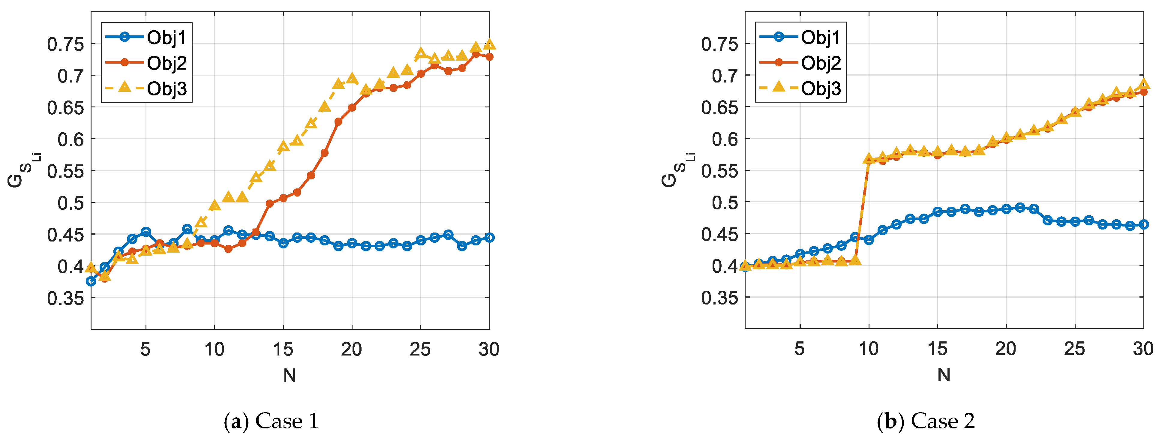
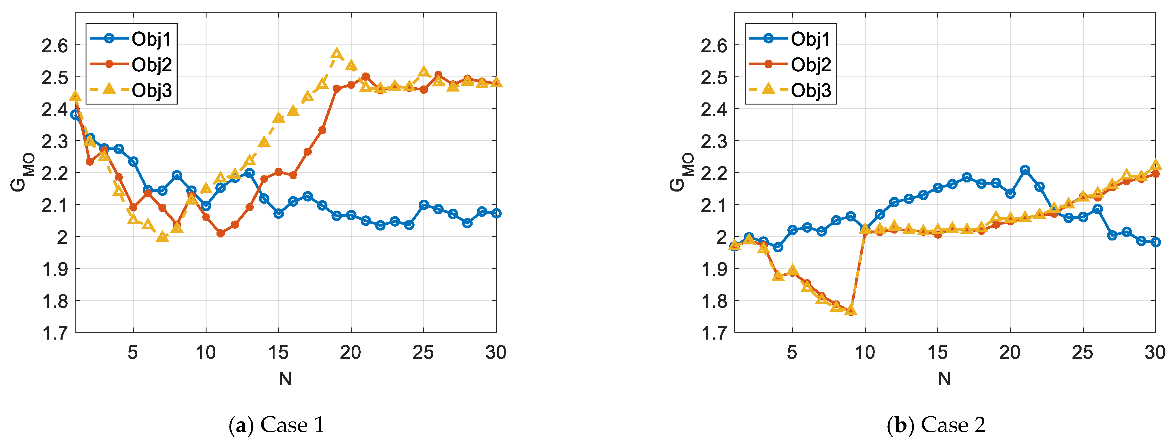
5.2.6. Index for Multi-Objective Problem
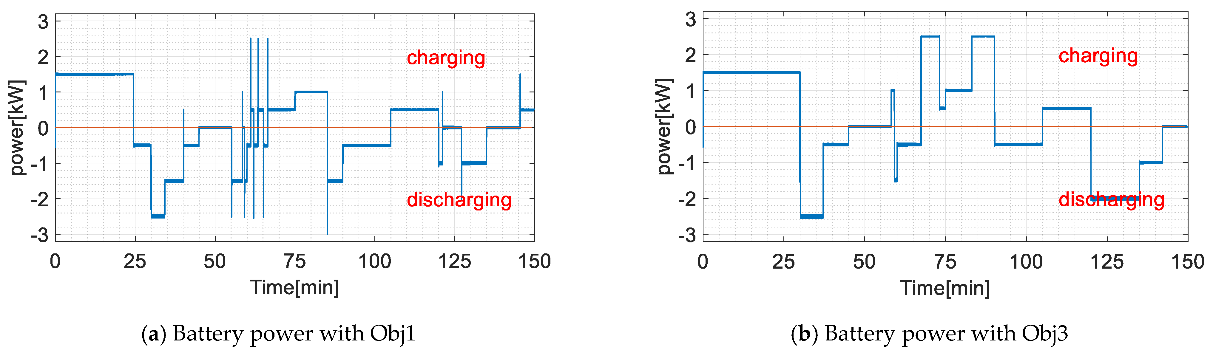
Although the performance of each objective function has been analyzed in (1)–(5) for each index, the overall performance of each objective function concerning the length of prediction horizon N still needs to be investigated. For a multi-objective problem with conflicting cost functions, e.g., JSOC and JSLi, there are trade-offs among the evaluation indices. Hence, weight parameters for each index are selected to represent the practical requirements, i.e., priorities of each optimization target. The final overall index is formed with the full knowledge of system performance throughout the whole operation, by using the above-mentioned indices, which are combined with appropriate user-specified weight parameters. The WFs utilized by the MPC to get the best overall results may differ from the weights used in the final evaluation. A neural network-based method in [46] is adopted for selecting WFs and weights in the overall index. The multi-objective evaluation index is presented in (28) with the adopted weights listed in Table 4.
G M O = ν S G S L i + ν δ G δ L i + ν S O C G S O C + v P b a t t G P b a t t + ν S O C R ¯ G S O C R ¯ + ν S O C R _ G S O C R _
Figure 8 presents the comparison of the proposed multi-objective evaluation index values with different prediction horizons and objective functions, as case 1 and case 2 show the results for adopting different load profiles. The figure shows that Obj2 and 3 can provide the optimal solutions with a shorter prediction horizon compared with Obj1. Compared to Obj2, Obj3 reaches a lower index value with a shorter horizon for load case 1. These results are heavily based on the selection of the weights for each index, but with the adjustment of the weights by the users according to their application requirements, the optimal objective function with a suitable prediction horizon can be selected.

5.3. Discussion

To summarize the results of the comparison study performed in the previous section, the best objective function for each evaluation index with short and long horizons are listed in Table 5. In addition, the performance change based on horizon selections of the objective functions in Section 5.2 is presented in the table.

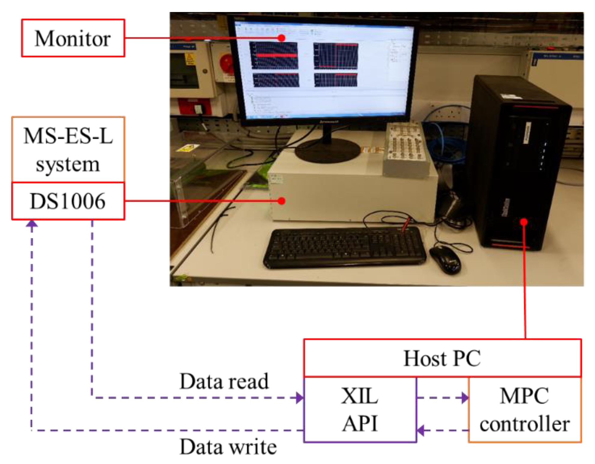
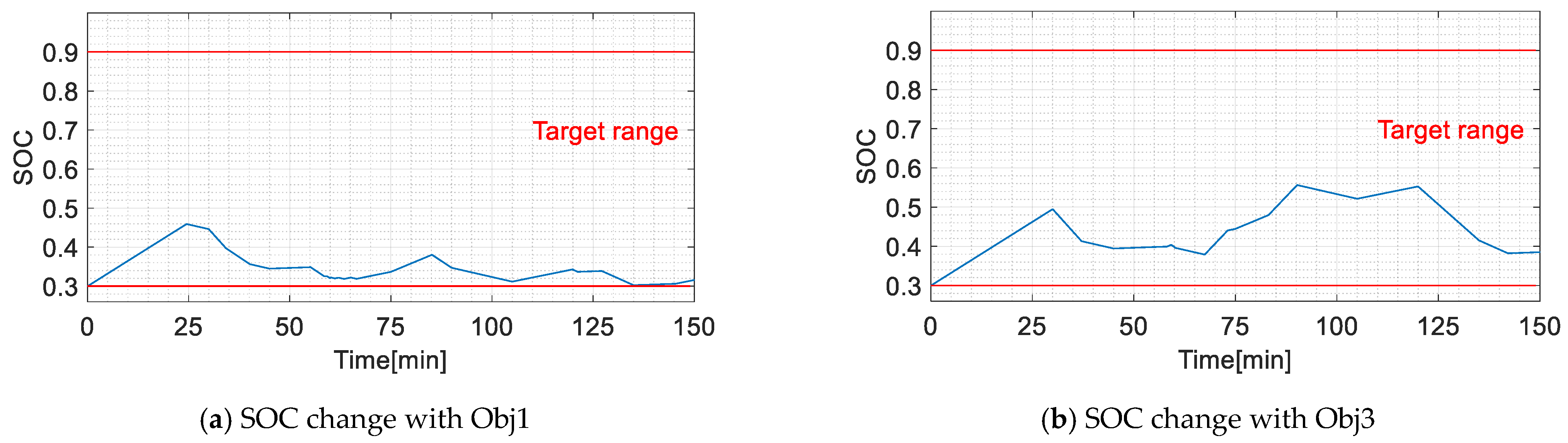
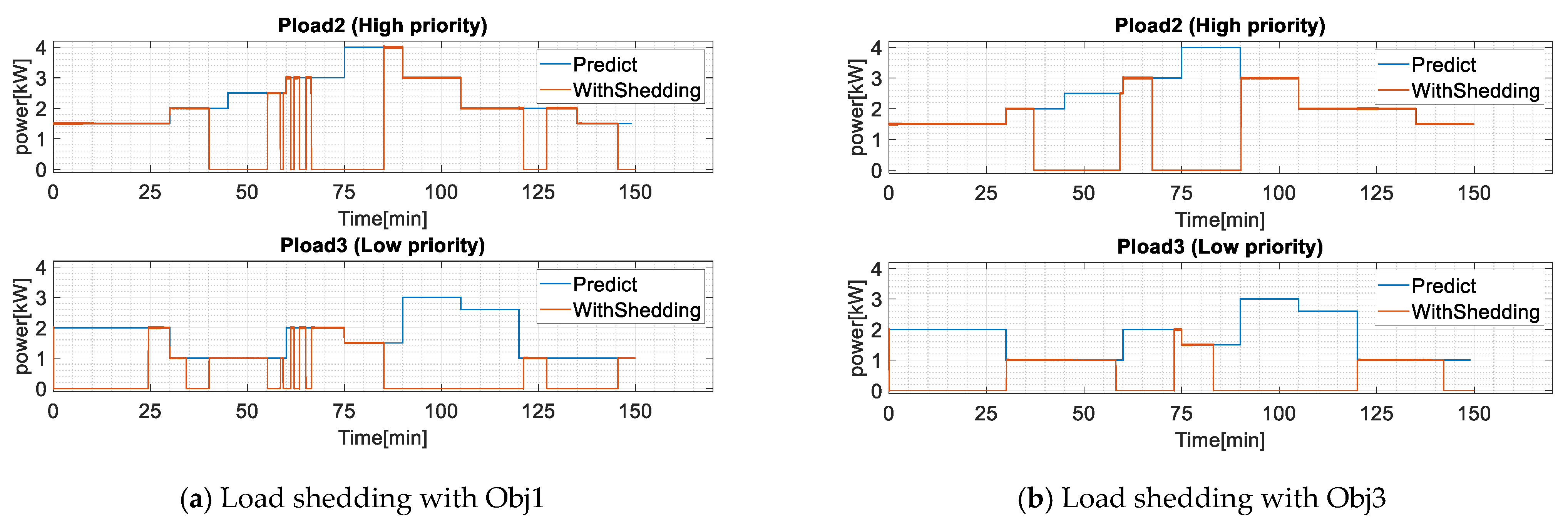
6. Real-Time Experiment

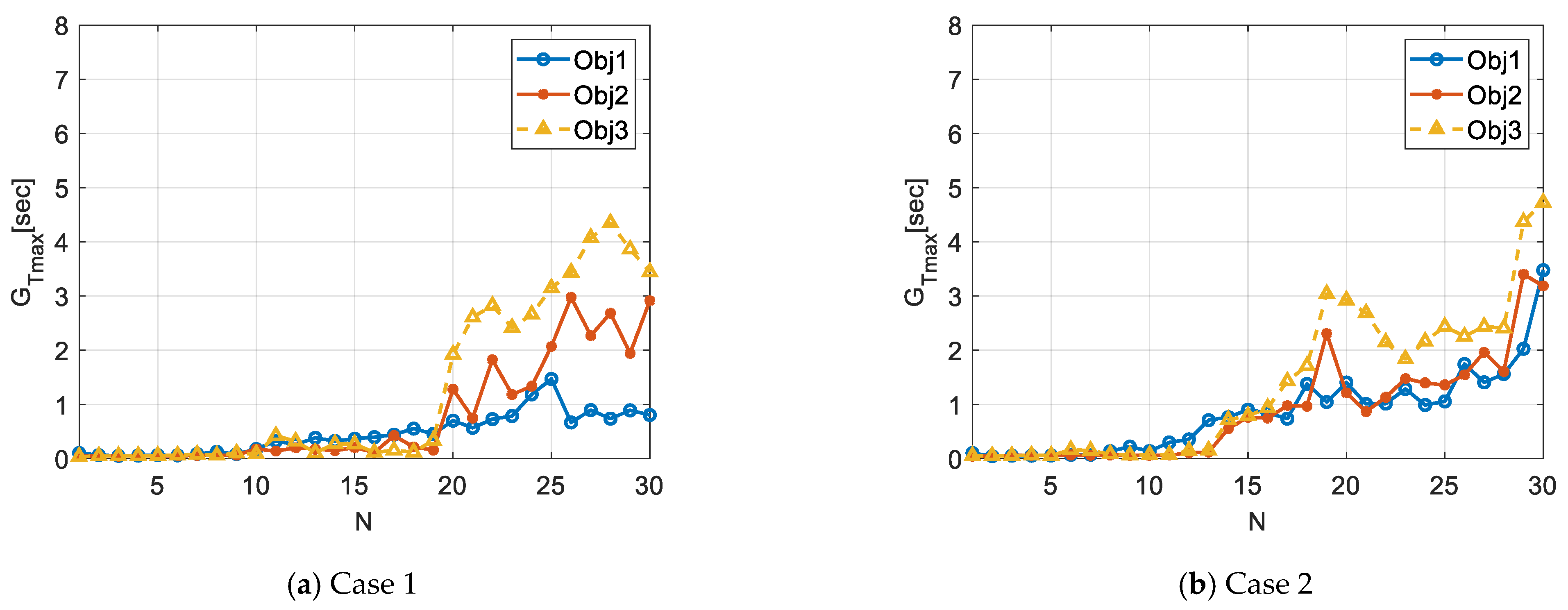
6.1. Computational Time Analysis

For real-time MPC applications, computation time is the key issue to be considered, as the time required to complete the computation should be less than the sampling time. When adopting the CPLEX solver, the computation time is influenced by several factors: (1) more complex models will often take longer time; (2) longer prediction horizons will take longer time; and (3) different input values, such as different load data as inputs to the MPC controller, can cause different computation times. Hence, to verify the MPC real-time application, the worst-case analysis of the computation time is conducted for Obj1–3. For each objective function and each N, the MPC controller will finally adopt 150 optimal solutions (one sample at each time step), and the maximum computation time for the MPC controller is recorded as the worst-case.
Figure 9 presents the maximum computation time GTmax changes for each objective function with respect to N. In both load cases, the maximum computation time for Obj1–3 has similar incrementally increasing tendencies as N increases: when N ≤ 10, the computation time is less than 0.2 s; when 10 < N ≤ 15, the computation time is less than 1s; and when 15 < N, the computation time will go above 1 s with the maximum value of less than 8 s. This indicates that the proposed MPC method could be adopted for real-time applications with selected sample times Ts larger than 10 s, during which the optimization would be completed, with the additional time being used for data measuring and communicating [49]. It is worth noting that a maximum computation time can be set in CPLEX. In this case, if the solver ran out of time, it would return the best solution that has been found in that time, rather than the optimal solution. In our case, Ts is set to 1 min because of the following reasons:
(1)
A 1-min sample time can provide the controller with enough time to obtain the measured status and updated load prediction, complete the optimization, and send the control signals to the system.
(2)
The proposed MPC method is mainly designed for satisfying the long-term battery SOC and load management requirements in the high-level control system. Since the SOC and average loads will not change very much in a few seconds, the MPC controller would not be required to update the control references frequently in small time intervals in the order of seconds. On the other hand, if the MPC is required to run every few seconds, to update the reference to cope with transients, the battery power and loads might change with every load fluctuation, which might cause instability in the system. In fact, instead of using MPC with long-term operating goals to act fast in response to the transient load changes, another real-time controller is usually added to the system at a lower control level, which will respond to the transient issues. This is the future work of the authors that will be presented in the future work discussion.
In summary, when adopting the proposed multi-objective evaluation index as the index for our overall preferred performance, Obj3 will have the best performance with a suitable prediction horizon (N = 7 and N = 9 for the corresponding load cases), with a computation time of lower than 0.2 s.

6.2. Real-Time Test

A real-time experiment was implemented in the lab at the Aerospace Technology Centre at the University of Nottingham, as presented in Figure 10. The MS-ES-L system was implemented in dSPACE 1006 for real-time simulation. The MILP-MPC controller was run in Matlab on a host PC, connected with the dSPACE. Every Ts, Matlab on the host PC uses the XIL API interface to read the measured data from dSPACE, including the load power PLi(k) and battery SOC(k). The MILP-MPC controller in Matlab takes these values as inputs and calls the CPLEX solver to provide the optimal power reference on the MS side Pin(k) and load shedding SLi(k). Finally, these optimal values are sent to the system implemented in dSPACE by the XIL API interface to realize real-time control. This experiment validates the suitability of the proposed system-level control framework for real-time implementation and the capability of the controller to provide the system with optimal control commands at specified control intervals to achieve the desired operating performance. It also verifies the coordination of the controller with the communication interfaces and local controllers at the lower level. This configuration (using PC and dSPACE) and using XIL API to read/write data and communicate between two levels, provides the opportunity to test the two-level control structure in real-time. The physical system and local controllers are running all the time and the system-level controller receives measurements from the system and updates its control commands on a regular basis (every one minute). In other words, they work in parallel. Otherwise, in a conventional series implementation with a PC and non-real-time simulation, the system and local controllers have to be stopped while running the system-level controller.
The control results of MPC with Obj1–Obj3 for all flight stages were compared in this experiment. During the flight, the loads were changed following the profile in Figure 3b. According to the analysis in Section 5, the MPC for Obj3 performed best when N = 9 with a computation time of less than 0.2 s. To verify this analytic conclusion based on the mathematical model, the MPC with Obj1–3 when N = 9 was applied in the experiment. The performance of each objective function can be visualized by observing the SOC changes, load shedding results, and battery power change. The real-time application of MPC was also verified. It should be noted that the flight-time slot was scaled down from the 60 s to 3 s to experiment within 7.5 min instead of 150 min. The battery capacity was accordingly scaled down to 0.2 kWh during the experiment. From both analyses in Figure 8 and the experiment, Obj2 and Obj3 had the same control results when N = 9 for this load profile. Hence, in the following comparisons, only the control results for Obj1 and Obj3 are considered, to study the differences.
Figure 11 presents the SOC measurement results during the flight stages, while (a) shows the results when MPC adopts Obj1, and (b) is related to Obj3. When Obj3 is adopted, the battery SOC is kept within 0.4–0.6 for the most time intervals with a maximum value of 0.56, while SOC is kept within 0.3–0.36 for the most time intervals when adopting Obj1, with a maximum value of 0.46. As the SOC is close to the lower limit when adopting Obj1, the system will be less stable for coping with unexpected failure scenarios.
The predicted and scheduled results for shedding of non-critical loads are presented in Figure 12, indicating load shedding in the system when adopting Obj1 in (a) and Obj3 in (b). The load contactors have more frequent on/off activities when adopting Obj1 compared to the case of adopting Obj2. Moreover, when adopting Obj1, the minimum time for keeping loads connected is 1 min, while Obj3 will keep loads connected for at least 8 min, which is preferred for reducing transient issues. Although Obj3 has less load on/off activities, it still has less load shedding time for both high and low priority loads: the load shedding index for Load 2 is 0.317 with Obj1 compared to 0.299 with Obj3, while the load shedding index value for Load 3 is 0.617 with Obj1 compared to 0.599 with Obj3. In conclusion, Obj3 outperforms Obj1 in both load shedding and switching activities in the experiment.
The battery charging/discharging power measurements are presented in Figure 13, where (a) presents the results with Obj1, while (b) presents the results with Obj3. Comparing the two figures, when adopting Obj3, the battery has fewer switching between the charging and discharging modes, and the charging/discharging power is less changed during each mode. In addition, the battery power curve with Obj1 has several transient peaks, which happen when Load2 is connected/disconnected simultaneously with the Load3 connection action being reversed. This verifies that Obj3 performs better in terms of battery lifecycle as well as system stability.
In summary, the MPC model with Obj1–3 proposed in Section 3 and Section 4 is applicable for real-time applications. In addition, it was found that the MPC with Obj3 performs better than Obj1 in the real-time experiment when N is selected as 9 for the given load profile. This supports the analysis and conclusions in Section 5.
This research inspires our future work when the system extends to the whole complex MEA power system configuration, such as HV buses, APU, multiple bidirectional converters, etc. A hierarchical controller based on the MPC method is proposed to cope with more operation constraints and scenarios, where the idea and findings mentioned in this work are adopted to design the objective function. Moreover, the model proposed for optimization in MPC can be extended to consider the effects of operating temperature and capacity fading in the battery model, which requires optimizing the battery charging/discharging power to reduce power losses and battery degradation. This topic will also be explored in our future research.

7. Conclusions

This paper proposed a system-level MPC framework to optimize the control and management of the energy storage and flexibility in the load-side for a MEA system. Following the control targets, three different objective functions were presented, and the importance of the different objective functions and prediction horizons was identified by analyzing the simulation results with the proposed evaluation framework including different performance indices. By assessing the impacts of different objectives, the paper provided the readers with a reference for selecting the most applicable objective function combination, as well as its potential impacts on deciding prediction horizons for different use cases.

Author Contributions

Conceptualization, X.W., J.A. and S.B.; methodology, X.W. and J.A.; software, X.W.; validation, X.W. and N.B.; formal analysis, X.W., J.A. and N.B.; investigation, X.W. and N.B.; resources, J.A. and S.B.; data curation, X.W.; writing—original draft preparation, X.W.; writing—review and editing, All; visualization, X.W.; supervision, J.A., S.B. and J.M.G.; project administration, S.B. and J.M.G.; funding acquisition, S.B. and J.M.G. All authors have read and agreed to the published version of the manuscript.

Funding

This work has been co-funded by the University of Nottingham and the Marie Skłodowska-Curie Actions co-funding of regional, national and international programmes (COFUND-DP) under the grant agreement number, 665468. Najmeh Bazmohammadi and Josep M. Guerrero are with the Center for Research on Microgrids (CROM) supported by VILLUM FONDEN under the VILLUM Investigator Grant (no. 25920).

Institutional Review Board Statement

Not applicable.

Informed Consent Statement

Not applicable.

Data Availability Statement

Data sharing is not applicable to this article.

Acknowledgments

The authors would like to thank the editor of the journal as well as three anonymous reviewers for their valuable and helpful comments. Further, the authors acknowledge the partnership agreement between Institute for Aerospace Technology at the University of Nottingham and CROM at the Aalborg University.

Conflicts of Interest

The authors declare no conflict of interest.

References

  1. Buticchi, G.; Bozhko, S.; Liserre, M.; Wheeler, P.; Al-Haddad, K. On-Board Microgrids for the More Electric Aircraft—Technology Review. IEEE Trans. Ind. Electron. 2018, 66, 5588–5599. [Google Scholar] [CrossRef] [Green Version]
  2. Damiano, A.; Porru, M.; Salimbeni, A.; Serpi, A.; Castiglia, V.; Di Tommaso, A.O.; Miceli, R.; Schettino, G. Batteries for Aerospace: A Brief Review. In Proceedings of the 2018 AEIT International Annual Conference, Bari, Italy, 3–5 October 2018; Volume 217. [Google Scholar] [CrossRef]
  3. Spagnolo, C.; Sumsurooah, S.; Hill, C.I.; Bozhko, S. Finite state machine control for aircraft electrical distribution system. J. Eng. 2018, 2018, 506–511. [Google Scholar] [CrossRef]
  4. Spagnolo, C.; Sumsurooah, S.; Hill, C.I.; Bozhko, S. Smart controller design for safety operation ofthe MEA electrical distribution system. In Proceedings of the IECON 2018—44th Annual Conference of the IEEE Industrial Electronics Society, Washington, DC, USA, 21–23 October 2018; Volume 1, pp. 5778–5785. [Google Scholar]
  5. Spagnolo, C.; Sumsurooah, S.; Bozkho, S. Advanced smart grid power distribution system for More Electric Aircraft application. In Proceedings of the 2019 International Conference on Electrotechnical Complexes and Systems (ICOECS), Ufa, Russia, 21–25 October 2019; pp. 1–6. [Google Scholar] [CrossRef]
  6. Chaouachi, A.; Kamel, R.M.; Andoulsi, R.; Nagasaka, K. Multiobjective Intelligent Energy Management for a Microgrid. IEEE Trans. Ind. Electron. 2013, 60, 1688–1699. [Google Scholar] [CrossRef]
  7. Arcos-Aviles, D.; Pascual, J.; Marroyo, L.; Sanchis, P.; Guinjoan, F. Fuzzy Logic-Based Energy Management System Design for Residential Grid-Connected Microgrids. IEEE Trans. Smart Grid 2016, 9, 530–543. [Google Scholar] [CrossRef] [Green Version]
  8. Zhang, H.; Saudemont, C.; Robyns, B.; Meuret, R. Comparison of different DC voltage supervision strategies in a local Power Distribution System of More Electric Aircraft. Math. Comput. Simul. 2010, 81, 263–276. [Google Scholar] [CrossRef]
  9. Motapon, S.N.; Dessaint, L.-A.; Al-Haddad, K. A Comparative Study of Energy Management Schemes for a Fuel-Cell Hybrid Emergency Power System of More-Electric Aircraft. IEEE Trans. Ind. Electron. 2013, 61, 1320–1334. [Google Scholar] [CrossRef]
  10. Panday, A.; Bansal, O.H. Energy management strategy for hybrid electric vehicles using genetic algorithm. J. Renew. Sustain. Energy. 2016, 8, 15701. [Google Scholar] [CrossRef]
  11. Francisco, R.; Roncero-Clemente, C.; Lopes, R.; Martins, J. Intelligent Energy Storage Management System for Smart Grid Integration. In Proceedings of the IECON 2018—44th Annual Conference of the IEEE Industrial Electronics Society, Washington, DC, USA, 21–23 October 2018; pp. 6083–6087. [Google Scholar] [CrossRef] [Green Version]
  12. Lin, C.-C.; Deng, D.-J.; Kuo, C.-C.; Liang, Y.-L. Optimal Charging Control of Energy Storage and Electric Vehicle of an Individual in the Internet of Energy With Energy Trading. IEEE Trans. Ind. Inform. 2017, 14, 2570–2578. [Google Scholar] [CrossRef]
  13. Ma, Y.; Yang, P.; Wang, Y.; Zhao, Z.; Zheng, Q. Optimal sizing and control strategy of islanded microgrid using PSO technique. In Proceedings of the 2014 IEEE PES Asia-Pacific Power and Energy Engineering Conference (APPEEC), Hong Kong, China, 7–10 December 2014; pp. 1–5. [Google Scholar] [CrossRef]
  14. Al-Saedi, W.; Lachowicz, S.W.; Habibi, D.; Bass, O. Power flow control in grid-connected microgrid operation using Particle Swarm Optimization under variable load conditions. Int. J. Electr. Power Energy Syst. 2013, 49, 76–85. [Google Scholar] [CrossRef]
  15. Pourmousavi, S.A.; Nehrir, M.H.; Colson, C.M.; Wang, C. Real-Time Energy Management of a Stand-Alone Hybrid Wind-Microturbine Energy System Using Particle Swarm Optimization. IEEE Trans. Sustain. Energy 2010, 1, 193–201. [Google Scholar] [CrossRef]
  16. Soares, A.; Gomes, A.; Antunes, C.H.; Oliveira, C. A Customized Evolutionary Algorithm for Multiobjective Management of Residential Energy Resources. IEEE Trans. Ind. Inform. 2016, 13, 492–501. [Google Scholar] [CrossRef]
  17. Logenthiran, T.; Srinivasan, D.; Shun, T.Z. Demand Side Management in Smart Grid Using Heuristic Optimization. IEEE Trans. Smart Grid 2012, 3, 1244–1252. [Google Scholar] [CrossRef]
  18. Shen, J.; Khaligh, A. A Supervisory Energy Management Control Strategy in a Battery/Ultracapacitor Hybrid Energy Storage System. IEEE Trans. Transp. Electrif. 2015, 1, 223–231. [Google Scholar] [CrossRef]
  19. Moreno, J.; Ortuzar, M.; Dixon, J. Energy-management system for a hybrid electric vehicle, using ultracapacitors and neural networks. IEEE Trans. Ind. Electron. 2006, 53, 614–623. [Google Scholar] [CrossRef]
  20. Parisio, A.; Rikos, E.; Tzamalis, G.; Glielmo, L. Use of model predictive control for experimental microgrid optimization. Appl. Energy 2014, 115, 37–46. [Google Scholar] [CrossRef]
  21. Parisio, A.; Rikos, E.; Glielmo, L. A Model Predictive Control Approach to Microgrid Operation Optimization. IEEE Trans. Control. Syst. Technol. 2014, 22, 1813–1827. [Google Scholar] [CrossRef]
  22. Parisio, A.; Wiezorek, C.; Kyntaja, T.; Elo, J.; Strunz, K.; Johansson, K.H. Cooperative MPC-Based Energy Management for Networked Microgrids. IEEE Trans. Smart Grid 2017, 8, 3066–3074. [Google Scholar] [CrossRef]
  23. Luna, A.C.; Diaz, N.L.; Graells, M.; Vasquez, J.C.; Guerrero, J.M. Mixed-Integer-Linear-Programming-Based Energy Management System for Hybrid PV-Wind-Battery Microgrids: Modeling, Design, and Experimental Verification. IEEE Trans. Power Electron. 2017, 32, 2769–2783. [Google Scholar] [CrossRef] [Green Version]
  24. Luna, A.C.; Meng, L.; Diaz, N.L.; Graells, M.; Vasquez, J.C.; Guerrero, J.M. Online Energy Management Systems for Microgrids: Experimental Validation and Assessment Framework. IEEE Trans. Power Electron. 2017, 33, 2201–2215. [Google Scholar] [CrossRef] [Green Version]
  25. Sockeel, N.; Shahverdi, M.; Mazzola, M. Impact of the State of Charge Estimation on Model Predictive Control Performance in a Plug-In Hybrid Electric Vehicle Accounting for Equivalent Fuel Consumption and Battery Capacity Fade. In Proceedings of the 2019 IEEE Transportation Electrification Conference and Expo (ITEC), Detroit, MI, USA, 19–21 June 2019. [Google Scholar] [CrossRef]
  26. Sockeel, N.; Shi, J.; Shahverdi, M.; Mazzola, M. Sensitivity Analysis of the Vehicle Model Mass for Model Predictive Control Based Power Management System of a Plug-in Hybrid Electric Vehicle. In Proceedings of the 2018 IEEE Transportation Electrification Conference and Expo (ITEC), Long Beach, CA, USA, 13–15 June 2018; pp. 767–772. [Google Scholar] [CrossRef]
  27. Fu, Z.; Li, Z.; Tao, F. Adaptive energy management strategy for hybrid batteries/supercapacitors electrical vehicle based on model prediction control. Asian J. Control. 2019, 22, 2476–2486. [Google Scholar] [CrossRef]
  28. Gomozov, O.; Trovão, J.P.; Kestelyn, X.; Dubois, M.R. Adaptive Energy Management System Based on a Real-Time Model Predictive Control With Nonuniform Sampling Time for Multiple Energy Storage Electric Vehicle. IEEE Trans. Veh. Technol. 2016, 66, 5520–5530. [Google Scholar] [CrossRef]
  29. Fortenbacher, P.; Mathieu, J.L.; Andersson, G. Modeling, identification, and optimal control of batteries for power system applications. In Proceedings of the 2014 Power Systems Computation Conference, Wroclaw, Poland, 18–22 August 2014; pp. 1–7. [Google Scholar] [CrossRef]
  30. Jiang, Z.; Raziei, S.A. Hierarchical Model Predictive Control for Real-Time Energy-Optimized Operation of Aerospace Systems. In Proceedings of the 2019 AIAA/IEEE Electric Aircraft Technologies Symposium (EATS), Indianapolis, IN, USA, 22–24 August 2019. [Google Scholar] [CrossRef]
  31. Seok, J.; Kolmanovsky, I.; Girard, A. Integrated/Coordinated Control of Aircraft Gas Turbine Engine and Electrical Power System: Towards Large Electrical Load Handling. In Proceedings of the 2016 IEEE 55th Conference on Decision and Control (CDC), Las Vegas, NV, USA, 12–14 December 2016; pp. 3183–3189. [Google Scholar]
  32. Leite, J.P.S.P.; Voskuijl, M. Optimal energy management for hybrid-electric aircraft. Aircr. Eng. Aerosp. Technol. 2020, 92, 851–861. [Google Scholar] [CrossRef]
  33. Zhang, Y.; Peng, G.O.H.; Banda, J.K.; Dasgupta, S.; Husband, M.; Su, R.; Wen, C. An Energy Efficient Power Management Solution for a Fault-Tolerant More Electric Engine/Aircraft. IEEE Trans. Ind. Electron. 2018, 66, 5663–5675. [Google Scholar] [CrossRef]
  34. Maasoumy, M.; Nuzzo, P.; Iandola, F.; Kamgarpour, M.; Sangiovanni-Vincentelli, A.; Tomlin, C. Optimal load management system for Aircraft Electric Power distribution. In Proceedings of the 52nd IEEE Conference on Decision and Control, Firenze, Italy, 10–13 December 2013; pp. 2939–2945. [Google Scholar] [CrossRef] [Green Version]
  35. Wang, W.; Koeln, J.P. Hierarchical Multi-Timescale Energy Management for Hybrid-Electric Aircraft. In Proceedings of the Dynamic Systems and Control Conference, Pittsburgh, PA, USA, 4–7 October 2020. [Google Scholar] [CrossRef]
  36. Aksland, C.T.; Alleyne, A.G. Hierarchical model-based predictive controller for a hybrid UAV powertrain. Control. Eng. Pr. 2021, 115, 104883. [Google Scholar] [CrossRef]
  37. Wang, X.; Atkin, J.; Hill, C.; Bozhko, S. Power Allocation and Generator Sizing Optimisation of More-Electric Aircraft On-board Electrical Power during Different Flight Stages. In Proceedings of the 2019 AIAA/IEEE Electric Aircraft Technologies Symposium (EATS), Indianapolis, IN, USA, 22–24 August 2019. [Google Scholar] [CrossRef]
  38. Ni, K.; Liu, Y.; Mei, Z.; Wu, T.; Hu, Y.; Wen, H.; Wang, Y. Electrical and Electronic Technologies in More-Electric Aircraft: A Review. IEEE Access 2019, 7, 76145–76166. [Google Scholar] [CrossRef]
  39. Chen, J.; Wang, C.; Chen, J. Investigation on the Selection of Electric Power System Architecture for Future More Electric Aircraft. IEEE Trans. Transp. Electrif. 2018, 4, 563–576. [Google Scholar] [CrossRef]
  40. Seresinhe, R.; Lawson, C. Electrical load-sizing methodology to aid conceptual and preliminary design of large commercial aircraft. Proc. Inst. Mech. Eng. Part. G J. Aerosp. Eng. 2014, 229, 445–466. [Google Scholar] [CrossRef]
  41. Barzegar, A.; Su, R.; Wen, C.; Rajabpour, L.; Zhang, Y.; Gupta, A.; Gajanayake, C.; Lee, M.Y. Intelligent power allocation and load management of more electric aircraft. In Proceedings of the 2015 IEEE 11th International Conference on Power Electronics and Drive Systems, Sydney, Australia, 9–12 June 2015; pp. 533–538. [Google Scholar] [CrossRef]
  42. Elkazaz, M.; Sumner, M.; Naghiyev, E.; Pholboon, S.; Davies, R.; Thomas, D. A hierarchical two-stage energy management for a home microgrid using model predictive and real-time controllers. Appl. Energy 2020, 269, 115118. [Google Scholar] [CrossRef]
  43. IBM. IBM ILOG CPLEX Optimization Studio OPL Language User’s Manual. Version 12, Release 8. Available online: https://www.ibm.com/docs/en/SSSA5P_12.8.0/ilog.odms.studio.help/pdf/opl_languser.pdf (accessed on 1 October 2021).
  44. Serale, G.; Fiorentini, M.; Capozzoli, A.; Bernardini, D.; Bemporad, A. Model Predictive Control (MPC) for Enhancing Building and HVAC System Energy Efficiency: Problem Formulation, Applications and Opportunities. Energies 2018, 11, 631. [Google Scholar] [CrossRef] [Green Version]
  45. Garche, J.; Jossen, A. Battery Management systems (BMS) for increasing battery life time. In Proceedings of the TELESCON 2000. Third International Telecommunications Energy Special Conference (IEEE Cat. No.00EX424), Dresden, Germany, 10 May 2000; pp. 85–88. [Google Scholar] [CrossRef]
  46. Wang, X.; Gao, Y.; Atkin, J.; Bozhko, S. Neural Network based Weighting Factor Selection of MPC for Optimal Battery and Load Management in MEA. In Proceedings of the 2020 23rd International Conference on Electrical Machines and Systems (ICEMS), Hamamatsu, Japan, 24–27 November 2020. [Google Scholar] [CrossRef]
  47. Zhang, Y.; Chen, J.; Yu, Y. Distributed power management with adaptive scheduling horizons for more electric aircraft. Int. J. Electr. Power Energy Syst. 2020, 126, 106581. [Google Scholar] [CrossRef]
  48. Australian Government Civil Aviation Safety Authority. Aircraft Electrical Load Analysis and Power Source Capacity; Australian Government Civil Aviation Safety Authority: Canberra, Australia, 2017.
  49. Behrooz, F.; Yusof, R.; Mariun, N.; Khairuddin, U.; Ismail, Z.H. Designing Intelligent MIMO Nonlinear Controller Based on Fuzzy Cognitive Map Method for Energy Reduction of the Buildings. Energies 2019, 12, 2713. [Google Scholar] [CrossRef] [Green Version]
Figure 1. The architecture of EPS under study.
Sustainability 13 13907 g001
Figure 2. Online MILP-MPC optimization procedure with receding horizon.
Sustainability 13 13907 g002
Figure 3. Different load cases.
Sustainability 13 13907 g003
Figure 4. Comparison of different prediction horizons and objective functions based on the normalized shedding index for two load cases.
Sustainability 13 13907 g004
Figure 5. Comparison of different prediction horizons and objective functions based on the contactor status change index for two load cases.
Sustainability 13 13907 g005
Figure 6. Comparison of different prediction horizons and objective functions based on the battery energy storage level index for two load cases.
Sustainability 13 13907 g006
Figure 7. Comparison of different prediction horizons and objective functions based on the battery power change index for two load cases.
Sustainability 13 13907 g007
Figure 8. Comparison of different prediction horizons and objective functions based on the multi-objective index for two load cases.
Sustainability 13 13907 g008
Figure 9. Comparison of the worst-case computation time of different prediction horizons and objective functions for two load cases.
Sustainability 13 13907 g009
Figure 10. Experimental setup.
Sustainability 13 13907 g010
Figure 11. SOC comparison for Obj1 and Obj3 when N = 9.
Sustainability 13 13907 g011
Figure 12. Load shedding comparison for Obj1 and Obj3 when N = 9.
Sustainability 13 13907 g012
Figure 13. Battery power comparison for Obj1 and Obj3 when N = 9.
Sustainability 13 13907 g013
Table 1. Nomenclature.
ParametersCost Function Terms
kTime intervals, k∈ℤ≥0JSLiCost function for minimizing total load shedding
HPrediction horizon (s)JδLiCost function for minimizing switching activities
TsSampling time (s)JPchCost function for maximining charging power
TTotal simulation time (s) JPdischCost function for minimizing discharging power
ηchdischBattery charging/discharging efficiency JΔCost function for keeping SOC within the target range
BcapBattery capacity (kWh)JSOCCost function for maximizing SOC to the upper bound
P c h max , P d i s c h max Maximum charging/discharging power (kW)JPbattCost function for minimizing battery power variations
LO/HILower/upper bounds of the battery SOC target rangeWeighting factors
P i n max Maximum input power from the MS-side (kW)wSWeighting factor for JSLi
P L i s h e d ( k ) The ith non-critical load power (kW)wδWeighting factor for JδLi
γLiThe priority of the ith non-critical loadwPchWeighting factor for JPch
NLiTotal number of non-critical loadswPdischWeighting factor for JPdisch
P L i n o n s h e d ( k ) The ith critical load power (kW)wΔWeighting factor for JΔ
Continues VariableswSOCWeighting factor for JSOC
Pin(k)Input power from the MS-side (kW)wPbattWeighting factor for JPbatt
Pch(k)Battery charging power (kW)Evaluation Indices
Pdisch(k)Battery discharging power (kW)GSLiEvaluation index for total load shedding
Pbatt(k)Battery overall power (kW)GδLiEvaluation index for contactor status change
SOC(k)Battery state of chargeGSOCEvaluation index for battery energy storage level
ε(k)Tolerance for lower bound of battery SOCGPbattEvaluation index for battery power variations
ϑ(k)Tolerance for upper bound of battery SOC G S O C R ¯ , G S O C R _ Evaluation index for SOC target range: upper and lower range bound correspondingly
Binary VariablesWeighting factors for multi-objective evaluation index
SLi(k)Contactor connection status of the ith non-critical loadvSWeight for GSLi
ζch(k)Indicator for charging the batteryvδWeight for GδLi
ζdisch(k)Indicator for discharging the batteryvSOCWeight for GSOC
vPbattWeight for GPbatt
v S O C R ¯ , v S O C R _ Weight for G S O C R ¯ ,   G S O C R _ correspondingly
Table 2. Parameters for the MS-ES-L system.
B c a p 4 kWh P c h max ,   P d i s c h max 4 kW
P i n max 4 kW η c h ,   η d i s c h 90%
P L o a d max 4 kWSOC(0)0.3
Table 3. Weighting factors in objective functions.
w S 5 w δ 34.7
w S O C 16 w Δ 1e5
w P b a t t 2 w P d i s c h 5.1
w P c h 3.1 in Obj1, 2.8 in Obj2 and Obj3
Table 4. Weights for the multi-objective index.
v s 2.8 v δ 1.68
v S O C 1 v P b a t t 0.4
v S O C R ¯ 104 v S O C R _ 104
Table 5. Objective function with the best performance and key features for each index when horizon changes.
IndexBest Obj with a Short HorizonBest Obj with a Long HorizonKey Features of Performance Tendency When Horizon IncreasesCombinations for Best Performance
Load sheddingObj2–Obj3Obj11. Performance of Obj1–Obj3 is better when a shorter horizon is applied (e.g., N < 10)
2. Performance of Obj2–Obj3 is reduced rapidly after the inflection point (N = 10) when horizon increases
Obj2–Obj3 with a short horizon (e.g., N < 10)
Contactor status changeObj2–Obj3Obj2–Obj31. Before the inflection point (N = 5), the performance of Obj1–Obj3 is improved rapidly when the horizon increases
2. After the inflection point, the performance has few changes when the horizon increases
Obj2–Obj3 at and after the inflection point (N ≥ 5)
Battery energy storage levelObj3Obj31. Performance of Obj1–Obj3 is better when a longer horizon is applied (e.g., N > 10)
2. Performance of Obj2–Obj3 is improved rapidly after the inflection point (N = 10) when horizon increases
Obj3 with a long horizon (e.g., N > 10)
Battery power changeObj3Obj31. Before the inflection point (N = 13), the performance of Obj2–Obj3 is improved when the horizon increases
2. After the inflection point, the performance of Obj2–Obj3 is reduced when the horizon increases
3. Obj1 doesn’t show relativity to horizon changes
Obj2–Obj3 at inflection point (N = 13)
Multi-objectiveObj2–Obj3Obj11. Before the inflection point (N = 9), the performance of Obj2–Obj3 is improved when the horizon increases
2. After the inflection point, the performance of Obj2–Obj3 is reduced when the horizon increases
3. Obj1 requires a long horizon to improve the performance (e.g., N > 25)
Obj2–Obj3 at inflection point (N = 9)
Publisher’s Note: MDPI stays neutral with regard to jurisdictional claims in published maps and institutional affiliations.

