Poverty Classification Using Machine Learning: The Case of Jordan

Abstract

The scope of this paper is focused on the multidimensional poverty problem in Jordan. Household expenditure and income surveys provide data that are used for identifying and measuring the poverty status of Jordanian households. However, carrying out such surveys is hard, time consuming, and expensive. Machine learning could revolutionize this process. The contribution of this work is the proposal of an original machine learning approach to assess and monitor the poverty status of Jordanian households. This approach takes into account all the household expenditure and income surveys that took place since the early beginning of the new millennium. This approach is accurate, inexpensive, and makes poverty identification cheaper and much closer to real-time. Data preprocessing and handling imbalanced data are major parts of this work. Various machine learning classification models are applied. The LightGBM algorithm has achieved the best performance with 81% F1-Score. The final machine learning classification model could transform efforts to track and target poverty across the country. This work demonstrates how powerful and versatile machine learning can be, and hence, it promotes for adoption across many domains in both the private sector and government.

1. Introduction

Goal 1 of the Sustainable Development Goals (SDGs) aims to end poverty in all its forms everywhere by 2030. However, the World Bank’s latest research indicates that the effects of the current COVID-19 pandemic will certainly appear in most countries until 2030. Under these conditions, the goal of reducing the absolute global poverty rate to less than 3 percent by 2030, which was already at risk before the crisis, is now far-fetched without swift, significant and substantial political action.

Poverty started to be seen as an issue in Jordan in the late 1980s [1]. Since then comprehensive poverty measurements have taken place. Using different methodologies, many studies have come to quite diverse estimates about the extent of poverty in the country. However, Jordanian officials have relied entirely on an absolute poverty line for measuring poverty. The absolute poverty line represents the cost of fulfilling a minimum of basic food and non-food needs. Hence, this measure is based on expenditure and not income. This means that a household is considered poor if it spends less than a certain amount per month on food and non-food products [2]. The most recent poverty line stood at 68 JD per person per month [3].

The poverty rate indicator is heavily used by the government of Jordan for monitoring and evaluating the poverty phenomenon. The poverty rate is defined as the percentage of the population falling below the absolute poverty line. The official estimated poverty rates for the years 2002, 2006, 2008, 2010, and lastly 2017 are 14.2%, 13%, 13.3%, 14.4%, and 15.7%, respectively. Official poverty statistics are produced using the nationally representative Household Expenditure and Income Survey (HEIS).

It is worth noting that the periodic national HEIS became representative on a sub-district level only in 2002 [2]. Special attention is devoted to several sub-districts in a joint report by the World Bank and the Ministry of Planning [4]. Some sub-districts are identified as poverty pockets as poverty is extreme reaching up to 75% of the population. The report acknowledged the fact that poverty pockets are located in sparsely populated desert areas.

The United Nations Development Programme (UNDP), which is a part of the United Nations Country Team (UNCT) in Jordan, attributes the latest increase in poverty rates to several challenges; unceasing public budget deficit, high inflation and low labour force participation rate in addition to the scarcity of natural resources. Tackling those socio-economic challenges requires a joint effort and support.

Household expenditure and income surveys provide data that is used for identifying and measuring the poverty status of Jordanian households. However, carrying out such surveys is hard, time consuming, and expensive. What is worse is that, by the time the data are collected and analyzed, it is often out of date, which means that policy makers are most likely to make decisions based on old data. Machine learning could radically change the game, making poverty measurement and identification cheaper and much closer to real-time.

This paper aims to give an idea about the scope of the poverty problem in Jordan since the early beginning of the new millennium. This will be achieved based on an accurate sample sufficient in its size and representative of all segments of Jordanian society, by relying on household expenditure and income surveys implemented by the Department of Statistics (DoS) for the years 2002, 2006, 2008, 2010, and lately 2017. The study also aims at producing initial and objective results with regard to building a machine learning model capable of predicting the poverty status of Jordanian households. This study is the first of its kind in the country.

In order to accurately estimate national level statistics regarding the economic status of households in a country, national-wide surveys collected from good representative samples are likely to be expensive and require huge efforts and hence, such surveys are scarce. Therefore, one can notice the tendency in the literature to look for other sources of data. One of these sources is satellite imagery [5,6,7,8]. A recent study applied machine learning and deep learning techniques with the aim of identifying features from the satellite imagery which could describe around 75% of the variation in local-level economic status [6], these techniques help understanding the well-being within a country as well as across countries [7]. Poverty maps were also generated from these satellite images, which are important for poverty targeting and public goods provision, specifically in low-income countries [8]. Similarly, street-level images were recently used to predict key livelihood indicators and it gives good results [9].

It has now become clear that a direct approach to measuring poverty through surveys is difficult, time consuming, and costly. After completing the fieldwork of the national HEIS, it usually takes two years to calculate the poverty line, compile data tables, and publish an analytical report [10]. Hence, there is an urgent need for a simple, accurate, and inexpensive tool to assess and monitor the poverty status of Jordanian households. Yet, when it comes to Jordan, this is an area that has received very little attention in the literature. In 2010 the scorecard approach is proposed [11]. The scorecard is built with a sub-sample of data from the 2006 HEIS. The design of the scorecard is kept simple, using ten indicators that are inexpensive to collect and straightforward to verify. Scores range from 0 (most likely below a poverty line) to 100 (least likely below a poverty line). Obviously, this approach cannot lead to a good generalization performance and it is also apparent that this approach is only valid for a certain period of time.

The contribution of this work is the proposal of an original machine learning approach to assess and monitor the poverty status of Jordanian households. This approach takes into account all the household expenditure and income surveys that took place since the early beginning of the new millennium. This approach is accurate, inexpensive, and makes poverty identification cheaper and much closer to real-time. The final model can be easily deployed and used by non-specialists to estimate the following:

• The probability of a household being poor.
• The poverty rate at a point in time.
• The change in poverty rate over time.

The remainder of this paper is organised as follows. Section 2 provides an overview of the materials and methods; data preprocessing is described in Section 3, Section 4 looks into the meaning of classification and how it can be linked to the poverty status of households, a number of classification algorithms are applied in Section 5 and some initial classification results are also presented, Section 6 is devoted to the issue of imbalanced data, final results are discussed in Section 7, and the paper finishes with some concluding remarks in Section 8.

2. Materials and Methods

2.1. Approach

In this study, well-known machine learning algorithms are applied to the poverty prediction problem. Because this research is the first of its kind in Jordan, the performance of known algorithms should be measured before starting to design new algorithms for this problem.

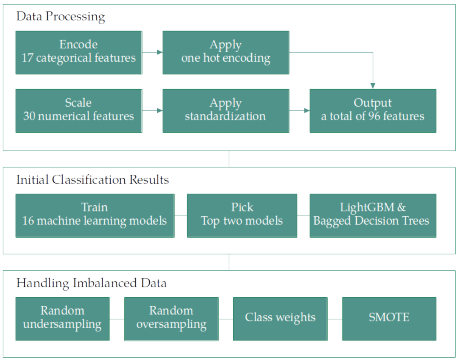
The research begins with the study and understanding of the dataset at hand, then deals with the problems presented in the data and suggests ways to address them. Then, the data are processed and fed to 16 machine learning algorithms. Finally, the results are presented and discussed.

Figure 1 presents a detailed representation of the flow followed in the study. The approach consists of three main phases which are explained in detail in the following sections.

2.2. Dataset

In order to increase the number of observations and have a better understanding of the scope of poverty in the country, the data collected by the DoS in five different national household expenditure and income surveys are combined and only the common features are used. This is shown in

Table 1. The dataset in numbers.

Year	Size
2002	10,558
2006	11,494
2008	10,956
2010	10,987
2017	19,216
Total	63,211

. The compiled dataset contains 63,211 household responses with 47 features (17 categorical features and 30 numerical features). These features are described in detail in

Table 2. Detailed description of the dataset features.

Name	Type	Description
Total_Expenditure	Numerical	Annually expenditure of all members of the household
Total_Income	Numerical	Annually income of all members of the household
Household_unit_area	Numerical	The area of the housing
Monthly_of_household	Numerical	Monthly house rent or the estimated value of the house if it is owned, for free or for work.
Age	Numerical	Household head age ($age$ $\ge 15$)
hh_size	Numerical	Household size
Child_Number	Numerical	Number of children ($age<18$) in the household
Adults_Number	Numerical	Number of adults ($15\le age<24$) in the household
Eldery_Number	Numerical	Number of elders ($age\ge 60$) in the household
Employed_Number	Numerical	Number of working members in the household ($age\ge 15$)
Number_of_rooms	Numerical	Number of all rooms in the house excluding the kitchen
kitchen	Categorical	Does the household have a kitchen?
Washing_machine_Number	Numerical	Number of owned washing machines
Refrigerator_Number	Numerical	Number of owned refrigerators
Freeze_Number	Numerical	Number of owned freezers
Gas_Oven_Number	Numerical	Number of owned gas ovens
Gas_oven_for_baking_Number	Numerical	Number of owned gas ovens for baking
Microwav_Number	Numerical	Number of owned microwaves
Dish_washer_Number	Numerical	Number of owned dishwashers
Vacuum_cleaner_Number	Numerical	Number of owned vacuum cleaners
T.V_Number	Numerical	Number of owned TVs
Satelite_recrivar_Number	Numerical	Number of owned dish receivers
Video_Number	Numerical	Number of owned video CDs/DVDs
Video_Camera_Number	Numerical	Number of owned video cameras
Computer_Number	Numerical	Number of owned computers
Internet_Connection	Categorical	Does the household have internet connection?
Telephone_Number	Numerical	Number of owned telephones
Mobile_Number	Numerical	Number of owned mobile phones
Fax_Number	Numerical	Number of owned fax
Air_conditioner_Number	Numerical	Number of owned air conditioners
Solar_water_heater	Categorical	Does the household have a solar water heater?
Sewing_Machine_Number	Numerical	Number of owned sewing machines
Private_Car_Number	Numerical	Number of owned private cars
sex	Categorical	What is the gender of the household head?
employed_status	Categorical	Does the household head work?
Nationality	Categorical	What is the nationality of the household head?
Educational_Level	Categorical	What is the educational level of the household head?
Marital_status	Categorical	What is the marital status of the household head?
aid	Categorical	Does the household receive an aid from any institution?
Material_wall_of_dwelling	Categorical	What is the material of the dwelling wall?
Type_of_dwelling_possession	Categorical	What is the type of dwelling possession
Main_source_of_heating	Categorical	What is the main source of heating?
Main_source_of_cooking	Categorical	What is the main source of cooking?
Type_of_sanitation	Categorical	What is the type of sanitation?
Urban_Rural	Categorical	Depends on the population density, urban if ≥5000, otherwise rural
gov	Categorical	Governorate of residence
poor_status	Categorical	Is the household poor?

.

2.3. Dataset Representativity

The DoS followed a two-stage stratified cluster sampling method when selecting the households for the HEIS [12]. In the first stage, the households are sampled with probabilities proportional to their size using the sampling frame provided by the population and housing census. At the same time, households for the field test and data collection are sampled using a systematic random sampling approach. In the second stage, eight and then four households are sampled. The latter four are sampled as replacements in case any of the first eight households refuses to participate in the survey. This provides a scientific and compelling way to ensure that the sample collected is a good representation of the Jordanian population.

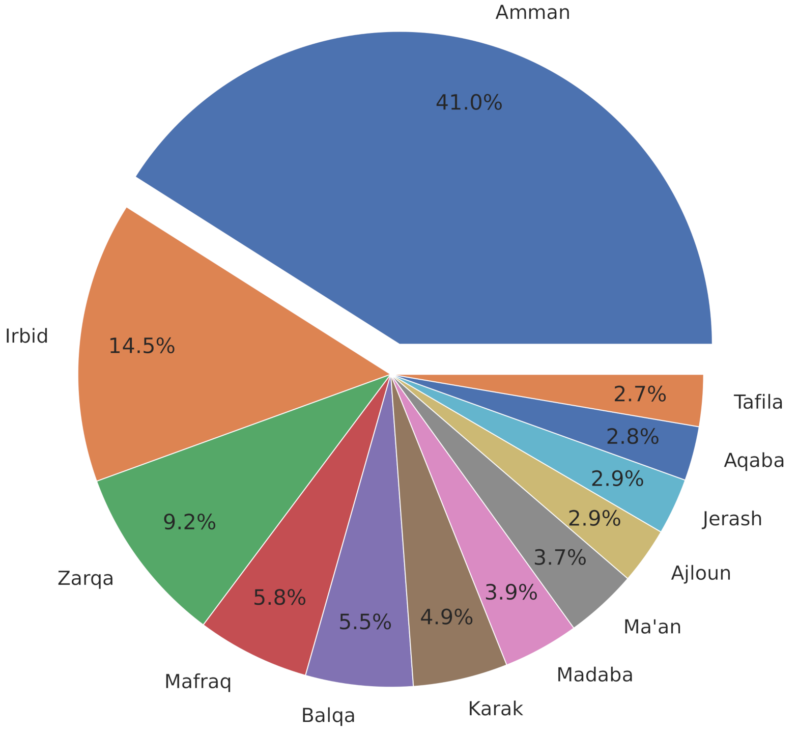
The geographic distribution of the sample collected showed a high participation rate from the three largest governorates in Jordan (41% Amman, 14.5% Irbid, and 9.2% Zarqa), which is proportional to the population size in these three major governorates. This is clearly illustrated in Figure 2, which also shows the participation rate for the rest of the governorates in the country.

2.4. Dataset Challenges

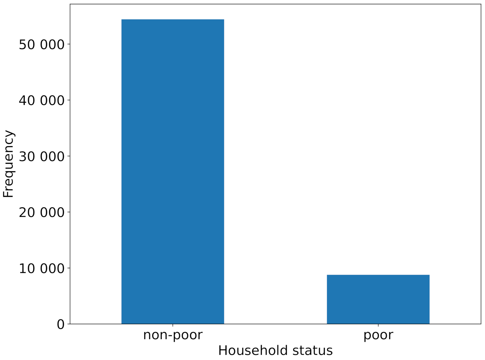
The data collected is highly imbalanced. The ratio of the poor to the non-poor is approximately 1:6 as shown in Figure 3. The number of the poor households is 8789 while the number of the non-poor households is 54,422. The class imbalance problem occurs when the class distributions are not represented equally. The infrequent class is most affected by this problem as low predictive accuracy is expected by many classification learning algorithms [13].

3. Data Preprocessing

Before applying any of the machine learning techniques to predict the poverty status of a household, the data need to be complete, clean, and in proper form. Data preprocessing is an important stage, which can improve the performance of the predictive model, in general, and can influence its accuracy [14]. The compiled data do not have any missing values, this is due to the approach followed by the DoS while collecting the information. Therefore, no imputation technique is required. However, the there are 17 categorical features that need to be transformed into numeric format. The common method used is one hot encoding technique [15] that will create a dummy variable for each value in each categorical feature, and use a binary encoding which indicates the existence of the value. After encoding all the categorical features, the dataset contains 96 features.

In order to test the accuracy of a predictive model (or compare the performance of different models) and provide an unbiased evaluation of the final model, a small proportion of the dataset needs to be saved for testing purposes. It is important to carefully select the testing set, in which it spans the various classes that a model would face when used in a real-world application. There are different splitting proportions; 70:30, 80:20 or 90:10. In this study, the training set consists of 90% of the data, while the remaining 10% is reserved for testing since the dataset is small and a large training set is needed. Furthermore, in order to fine-tune a model’s hyper-parameters, a validation set is needed. The validation set is part of the training set; usually 10%. This division was accomplished using a stratified technique [16].

Finally, it is important before bringing the data into a machine learning model to have all the features on a comparable scale, since this unscaled data can cause inaccurate or false predictions. In this study, standardization, normalization, and a combination of both are applied. Normalization is a scaling technique in which values are shifted and rescaled so that they end up ranging between 0 and 1 using the formula in (1) [14]. Standardization is another scaling technique where the values are centered around the mean with a unit standard deviation using the formula in (2) [17].

$$X^{\prime }=\frac{X-X_{min}}{X_{max}-X_{min}}$$

(1)

where $X_{max}$ and $X_{min}$ are the maximum and the minimum values of a feature, respectively.

$$X^{\prime }=\frac{X-\mu }{\sigma }$$

(2)

where $\mu$ is the mean of feature values and $\sigma$ is the standard deviation of the feature values.

4. Classification Algorithms

Classification is a type of supervised machine learning, in which an observation, in this case: a household survey response, is classified into one of two classes (poor and non-poor) based on a number of predictive features. There are many classification algorithms that can be applied to the problem at hand, and thus it is quite challenging to choose the right algorithm as many factors control the process. Data-related aspects, and problem-related aspects form the decision criteria. Even for an experienced data scientist a variety of machine learning algorithms are normally explored before finding an appropriate algorithm for a specific problem. Some of the most commonly used machine learning algorithms are applied next.

5. Initial Classification Results

Once faced with a new predictive modeling problem, a quick and objective assessment is needed to evaluate a diverse set of algorithms. This is an essential step in the process of applied machine learning that can lead to a useful first cut results and determine the types of algorithms that may be worth to explore further. This technique is known as spot-checking algorithms [18].

In this section, 16 different classification algorithms are applied (

Table 3. Classification algorithms: Abbreviations and parameters used.

Algorithm	Abbreviation	Parameters
Logistic Regression [20]	logistic	Default parameters
Ridge Regression [21]	ridge	alpha = $[0.1,1]$ with a step size of 0.1
Stochastic Gradient Descent [22]	sgd	maxiter = 1000, tol = 0.001
Passive Aggressive [23]	pa	Default parameters
k-Nearest Neighbors [24]	knn	Default parameters
Decision Tree [25]	cart	Default parameters
Extra Tree [26]	extra	Default parameters
Support Vector Machine [27]	svml svmp svmr	kernel = ’linear’ kernel = ’poly’ C = $[0.1,1]$ with a step size of 0.1
Naive Bayes [28]	bayes	Default Gaussian Naive Bayes parameters
AdaBoost [29]	ada	n_estimators = 100
Bagged Decision Trees [30]	bag	n_estimators = 100
Random Forest [31]	rf	n_estimators = 100
Extra Trees [26]	et	n_estimators = 100
Gradient Boosting Machine [32]	gbm	n_estimators = 100
Light GBM [33]	lgbm	n_estimators = 100
Scalable Tree Boosting System [34]	xgb	n_estimators = 100

). In order to make sure that features are on the same scale, feature scaling is performed using the three different approaches outlined earlier, standardization, normalization, and a combination of both. One can notice from Table 3 that some of the algorithms are slightly modified; in particular Ridge Regression and SVM. The different classification algorithms are evaluated using the stratified 10-fold cross validation. The performance of each algorithms is assessed using the mean of the f1-score [19].

$$\begin{array}{cc}\hfill \mathrm{mean}{f}_1\mathrm{score}& =\frac{1}{N}\sum _{i=1}^N{f}_1\hfill \\ \hfill f_1& =\frac{\mathrm{tp}}{\mathrm{tp}+\frac{1}{2}(\mathrm{fp}+\mathrm{fn})}\hfill \end{array}$$

(3)

where N is the number of observations in the testing set, tp is the true positives, fp is the false positives, and fn is the false negatives.

The specifications of the platform on which experiments are performed are shown in

Table 4. Specifications of the experimental platform.

Aspect	Specification
CPU	Intel(R) Core(TM) i7-4980HQ CPU @ 2.80 GHz
GPU	Nvidia GeForce GTX 980 M
Memory	32 GB DDR3 @ 1600 MHz
OS	Ubuntu 20.04 LTS, 64-bit
Libraries	Python 3.8.5, scikit-learn 0.23.2, lightgbm 3.1.0, xgboost 1.2.0

. Experiments are conducted on the CPU since the GPU does not give better speedup.

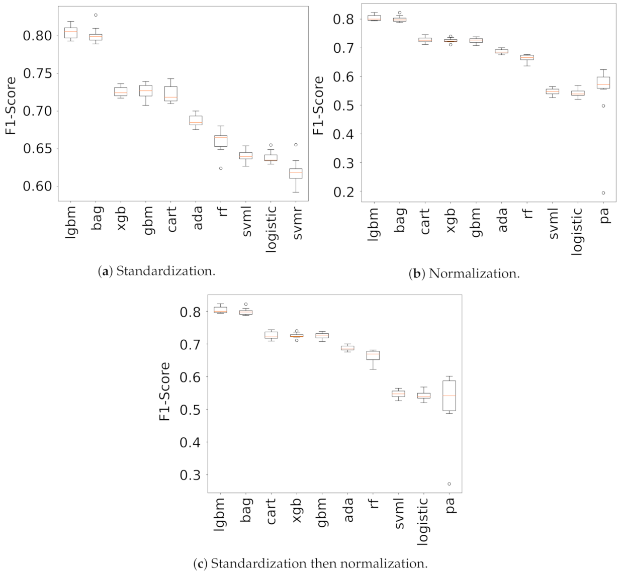
The performance of the top ten well-performed algorithms is shown in Figure 4. One can clearly notice that regardless of the scaling approach that is used, LightGBM and Bagged Decision Trees algorithms outperform the rest of the classification algorithms. Hence, these two machine learning algorithms are a good place to focus our attention on. One can also conclude from Figure 4 that the final machine learning model will likely to show a performance of at least 80% f1-score.

As LightGBM and Bagged Decision Trees are the top two well performing algorithms with f1-score around 80%, these two algorithms will be considered in the next few sections taking into account the standardization technique.

6. Handling Imbalanced Data

Imbalanced data are typically associated with classification problems where the different classes are not represented equally. For example, in this dataset, there are 86.1% (n = 54,422) non-poor households, while, only 13.9% (n = 8789) poor households. Although machine learning algorithms have shown great success in many real-world applications, learning from imbalanced data are still not fully developed yet [35]. Often, learning from imbalanced data are referred to as imbalanced learning [36]. The problem of imbalanced data has attracted the attention of many researchers over the last decade, and hence, numerous specialized methods have been proposed [36,37,38]. In general, these methods can be categorized into two main groups. The first group focuses on the data itself by trying to enhance the distribution of the data. While the second group focuses on modifying the machine learning algorithm instead of the data itself. The two approaches are used in this work.

For the current data, four techniques (three from the first group and one from the second group) are used to handle the highly imbalance ratio. The first technique is known as random over-sampling, in which a random portion of the minority class is selected and duplicated. The second technique, on the other hand, is known as random under-sampling, in which a random portion of the majority class is eliminated. The third technique is known as Synthetic Minority Over-sampling Technique (SMOTE), which is similar to the random over-sampling, however, instead of duplicating a random portion of instances, this technique generates a portion of synthetic instances. Finally, a technique known as class weights, which belongs to the second group, is also used. This technique assigns weights on the cost function to give an importance to a class over the other.

6.1. Random Oversampling

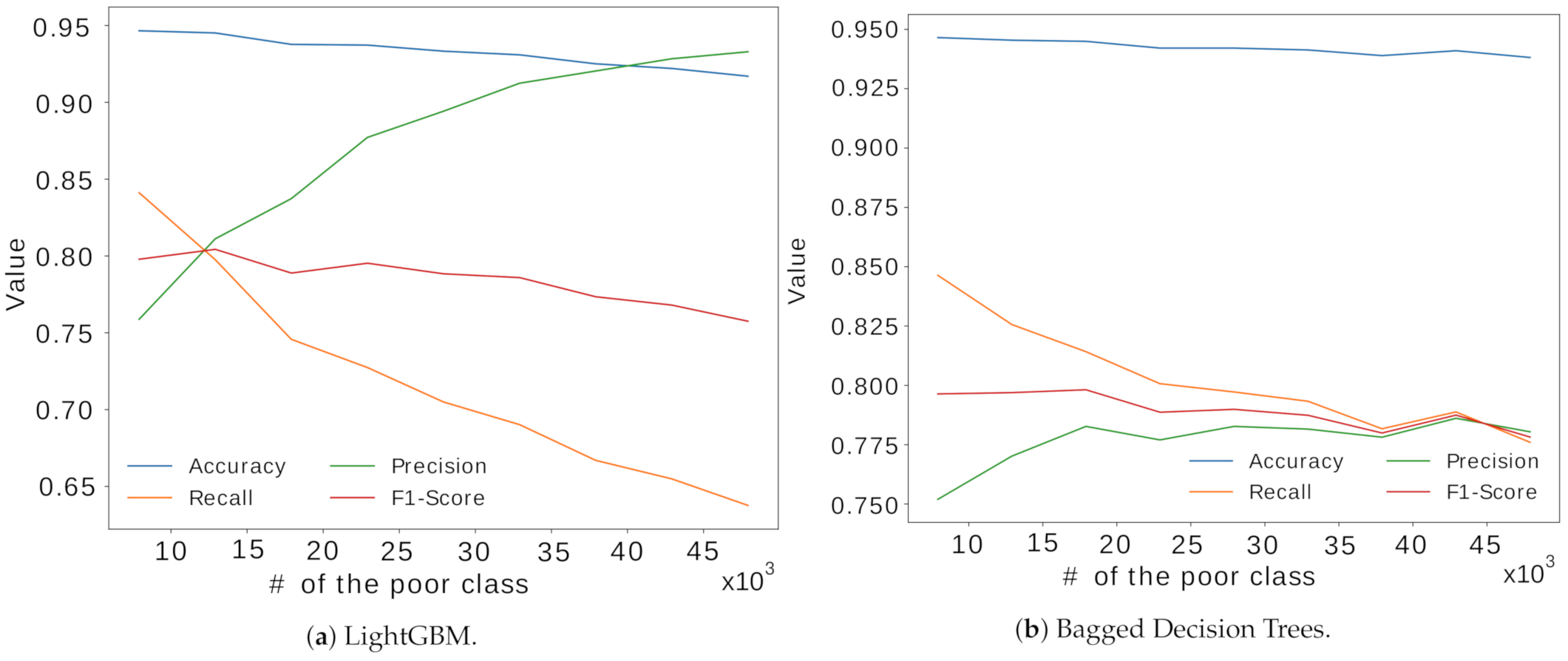
The way this technique works is by duplicating instances in the minority class. Thus, the minority class will have a better chance to be detected by a machine learning algorithm. By oversampling, the performance of a machine learning algorithm improves in identifying patterns that distinguish a number of classes [39]. More importantly, there is no information loss. However, when instances in the minority class are duplicated this may lead to the problem of overfitting [40]. The top two well-performing algorithms presented earlier, LightGBM and Bagged Decision Trees are used here for evaluation. The random oversampling technique is run multiple times for different number of instances and some performance measurements are assessed. The best number of instances that gives the best F1-score for the LightGBM and Bagged Decision Trees methods are 13,000 and 17,000, respectively (Figure 5).

6.2. Random Undersampling

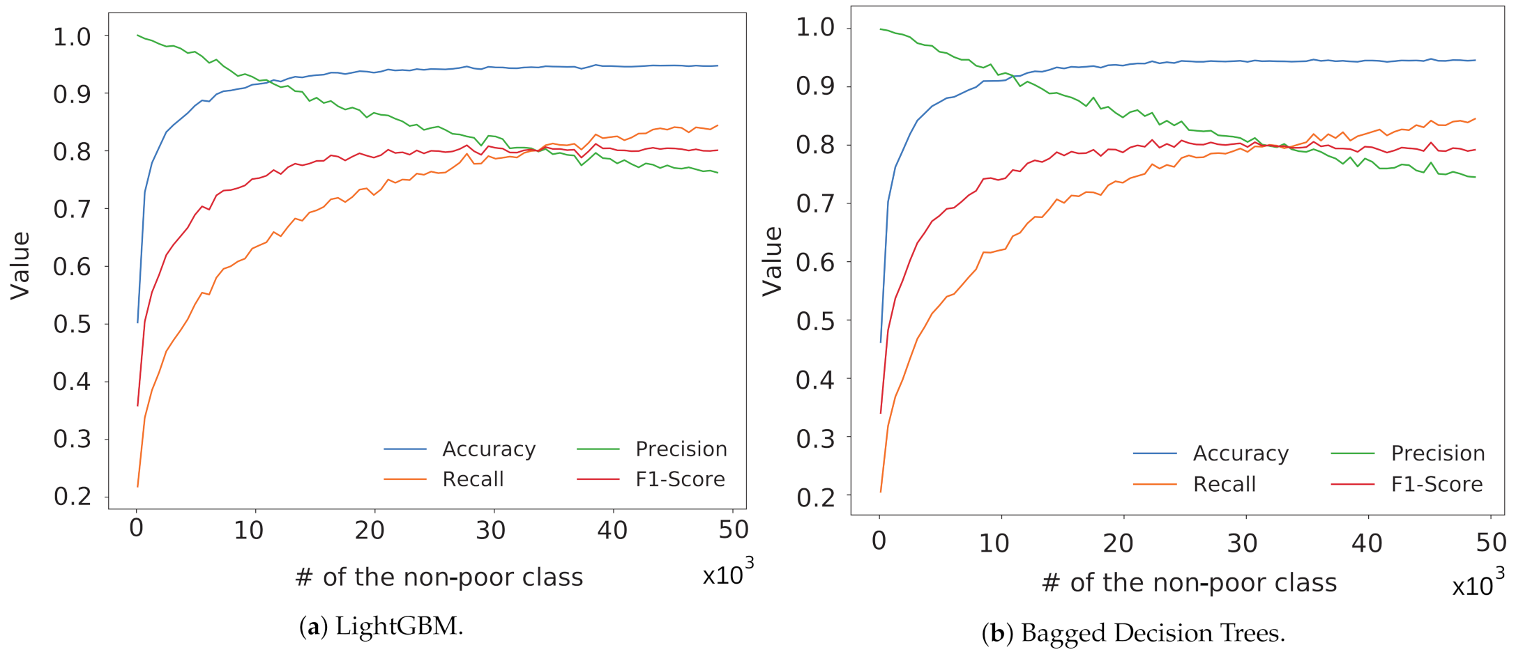
In this technique a random number of instances are eliminated from the majority class with the aim of improving the performance of a machine learning algorithm. This technique, however, has its own pros and cons. While this technique can be computationally efficient as the number of training data are reduced, there is a risk of information loss, or even worse, the dataset may become less representative. Similar to the oversampling, the random undersampling technique is run multiple times and some performance measurements are assessed. The number of instances that gives the best F1-scores is approximately 33,000 for both algorithms, the LightGBM and Bagged Decision Trees (Figure 6).

6.3. Synthetic Minority Over-Sampling Technique (SMOTE)

The real motivation behind this technique is to overcome the challenging problem of overfitting that may result from the random oversampling technique [41]. This is achieved through generating synthetic instances instead of duplicating already existed instances. Nevertheless, the SMOTE can introduce noise to the data, since neighboring instances can be from other classes [42].

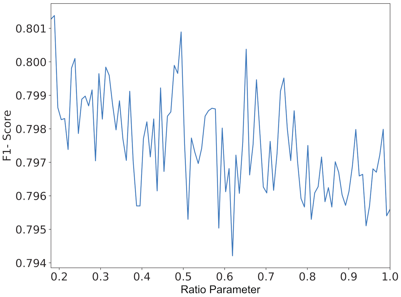
One of the main steps of the SMOTE is to determine a ratio parameter between 0 and 1. This ratio parameter tells the algorithm to sample the minority class to a desired number of data points. However, increasing the number of data points using SMOTE does not guarantee accurate results. Hence, different percentages need to be experimented. This can be accomplished using grid search. A stratified 3-fold cross validation in addition to the f1-score as a parameter for performance evaluation are used. The LightGBM algorithm is used here due to its computational efficiency [33]. Despite the oscillatory F1-Score as the ratio parameter is increased from 0.18 to 1 (Figure 7), it is obvious that an optimal ratio parameter can be found around 0.19, which upsample the minority class to around 10,340 (number of data points in the majority class 54,422 × optimal ratio parameter 0.19).

6.4. Class Weights

The idea of this technique is quite simple—the class imbalance problem is approached by simply providing a weight for each class and thus placing more emphasis on the minority class. This will eventually result in a classifier that can learn equally from both classes. For the current data, the expected class weights ratio is 6:1 which is inversely proportional to the actual ratio of the poor class to the non-poor class. However, it is not guaranteed that this ratio will give an optimal performance hence, other approaches should be considered.

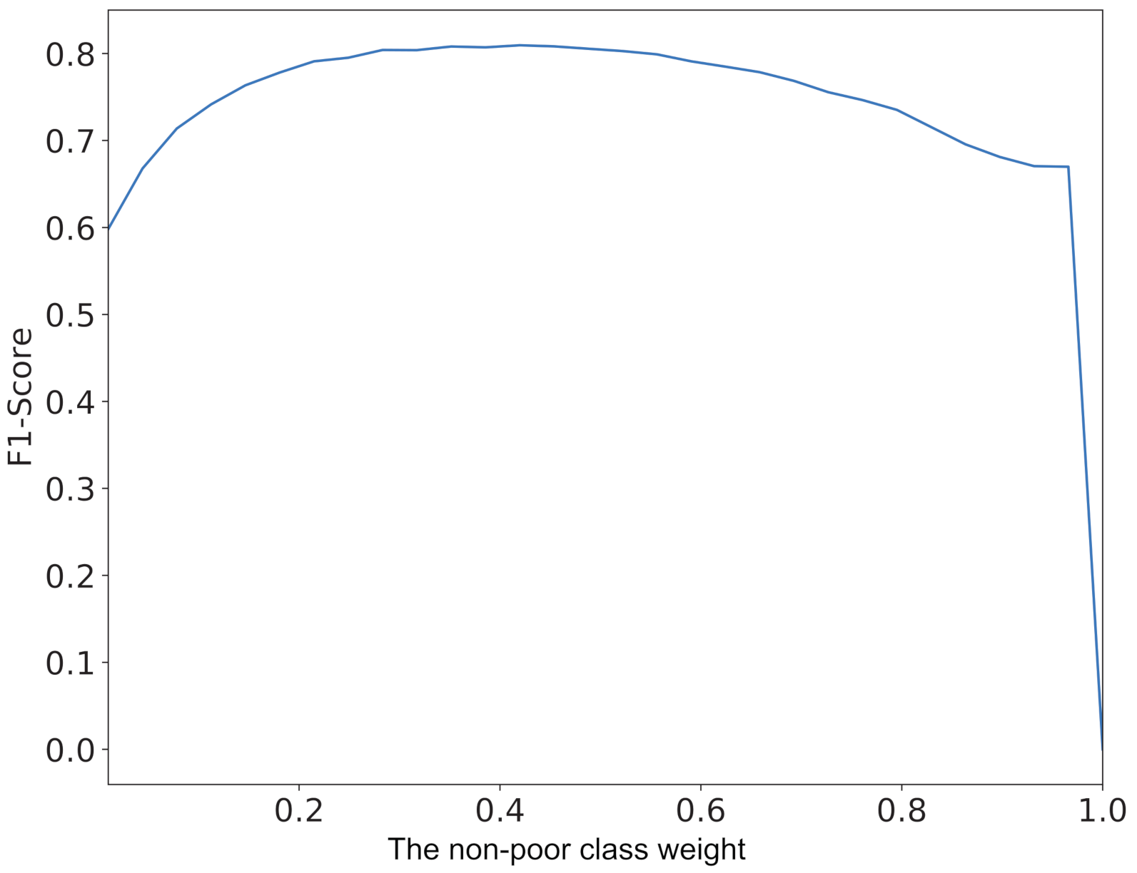
An alternative approach is to try different ratios of the class weights. This can be accomplished using grid search [43]. A stratified 5-fold cross validation in addition to the f1-score as a parameter for performance evaluation are used, while searching for a proper ratio of the class weights. Note that the LightGBM algorithm is used here due to its computational efficiency [33]. This is illustrated in Figure 8. According to Figure 8, the performance of the LightGBM algorithm is steadily improving until it reaches a certain weight (0.42). Then the performance decreases until it reaches a weight of 1 that is associated with a very low value of the f1-score (nearly zero). It is worth noting that the weight of 1 means that the algorithm puts all the weight on one class while neglecting the other. Therefore, the optimal weights are 0.58 to the poor class, and 0.42 to the non-poor class.

7. Results and Discussion

After the dataset was prepared by converting categorical data into numerical data using one hot encoding, the next step was to bring all the features on comparable scale. The latter was approached by standardization, normalization, and a combination of both. The initial classification results in Section 5 showed that Standardization resulted in a slightly better performance, and thus it has been adopted in this section for further analysis. The class imbalance problem that the dataset suffers from was also investigated in Section 5. Random oversampling, random undersampling, SMOTE, and class weights are applied here in this section for this challenging task.

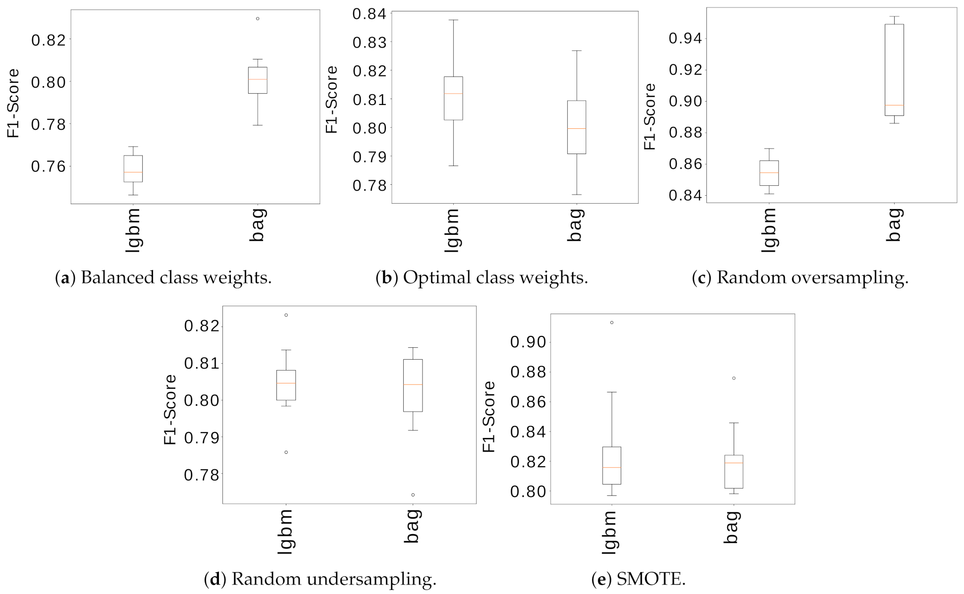
The evaluation process starts with the stratified 10-fold cross validation applied to the new training set that is obtained from the four methods discussed in the previous section for dealing with class imbalance. The top two well performing algorithms presented earlier in Section 5, LightGBM and Bagged Decision Trees, are used here to compare the four methods. This is illustrated in Figure 9. Then the evaluation process proceeds to evaluate the performance of these two algorithms using the test set. The results of this evaluation are presented in

Table 5. Performance evaluation: Testing set.

Method	F1-Score
	LightGBM	Bagged Decision Trees
Class weights (balanced)	0.75	0.79
Class weights (grid search)	0.80	0.80
Random oversampling	0.81	0.79
Random undersampling	0.80	0.79
SMOTE	0.80	0.79

.

A few remarks can be made regarding the results shown in Figure 9 and Table 5. The first remark is that the 6:1 class weights ratio (which is inversely proportional to the actual ratio of the poor class to the non-poor class) does not necessarily imply achieving the best performance. This can be clearly seen in Figure 9a,b. For the LightGBM algorithm, the optimal class weights is able to achieve slightly over 81% F1-Score, yet for the same algorithm, the balanced class weights struggles to achieve a 76% F1-Score.

The second remark is regarding the performance of LightGBM and Bagged Decision Trees where the occurrence of overfitting is obvious for the random oversampling technique. Both algorithms show high F1-Score values for the training set in Figure 9c, however, when the performance of both algorithms is evaluated using the testing set, the F1-Score is significantly decreased as shown in Table 5, especially for the Bagged Decision Trees.

The third remark is regarding the random under sampling and SMOTE techniques. The LightGBM and Bagged Decision Trees show a close performance for the training set as shown in Figure 9d,e. When both algorithms are evaluated using the testing set, an 80% F1-Score is achieved by the LightGBM for both techniques and 79% is achieved by the Bagged Decision Trees also for both techniqus. This is clearly shown at the botton of Table 5.

More importantly, however, the final remark here is that there is no significant difference in the performance of the two algorithms, LightGBM and Bagged Decision Trees, before and after applying the imbalanced data techniques. Therefore, one can conclude that the initial classification results presented in Section 5 were sufficient.

It is worth noting that the approach adopted and followed to arrive at these final results is independent of the data itself and is considered a general approach. Hence, researchers can always adopt the same approach to arrive at conclusions tailored to fit their own data.

With the aim of helping and supporting policy makers and international donors to alleviate food insecurity in Afghanistan, two machine learning classification models, classification decision tree and random forest model, are used and applied to a household survey. The final model is able to accurately identify 80% of food-insecure household [44]. In a similar study, a number of machine learning classification algorithms are used as an approach to identify poor households as the potential receiver of poverty alleviation programs. Poverty data are extracted from the dataset of Lagangilang, Abra, Philipppines. In order to get the best predictive model, the different classification algorithms are evaluated based on a number of performance metrics. The machine learning classification algorithms have an average F1-Score of 87% [45]. It is quite apparent that the approach adopted in this study and the final results obtained are totally acceptable in the scientific literature.

This work is an initial step towards helping and supporting the Jordanian government and local civil society organizations, in addition to foreign organizations in their endeavor to reduce poverty. A machine learning model can be used as a tool to assess and monitor the poverty status of Jordanian households. The model can be easily deployed and used by non-specialists. It should be mentioned, however, that this model is unique and only valid for Jordan. Though, it would be interesting to see how accurate the model is when applied to other countries with similar poverty trends to Jordan. One notable avenue for future work is to consider feature selection to select those features which contribute most to the prediction of the poverty level of households.

Once the responses of households are collected the deployed model can be easily used by the Jordanian government, local civil society organizations, and foreign organizations to estimate the probability of a household being poor, the poverty rate at a point in time, and the change in poverty rate over time.

During the past twenty years, Jordan has been exposed to many exceptional circumstances, such as hosting large numbers of refugees from neighboring countries and for different periods of time. Such circumstances had a clear and tangible effect on the pattern of household income and expenditure, which was documented through field surveys. The model proposed in this study is trained on the data extracted from these surveys. Therefore, one can conclude that the model is able to take into consideration any emerging crises or abnormal conditions.

To achieve the desired goals of this study and to achieve sustainability, it is imperative that policy-makers, in addition to local civil society organizations, and foreign organizations concerned with combating poverty invest in this type of proposals and strive to implement it on the ground.

8. Conclusions

This work sheds a light on the multi-dimensional phenomenon of poverty in Jordan. Analyzing and utilizing poverty data from several national household surveys are the highlights of this work.

An original machine learning approach to assess and monitor the poverty status of Jordanian households is presented. This approach takes into account all the household expenditure and income surveys that took place since the early beginning of the new millennium. The final model can be easily deployed and used by non-specialists to estimate the probability of a household being poor, the poverty rate at a point in time, and the change in poverty rate over time.

In total, 16 different machine learning classification algorithms are evaluated. LightGBM and Bagged Decision Trees showed a superior performance over the rest of the learning algorithms. The datasest used is sufficient in its size and representative of all segments of Jordanian society. The data collected by the DoS in five different national household expenditure and income surveys were combined and only the common features were used.

The dataset is prepared by converting categorical data into numerical form using one hot encoding in addition to bringing all the features on comparable scale. The latter is approached by standardization, normalization, and a combination of both. Standardization resulted in a slightly better performance, and thus it has been adopted. The class imbalance problem that the dataset suffers from has been also investigated. Random oversampling, random undersampling, SMOTE, and class weights were applied for this challenging task.

The final machine learning classification model has achieved an accuracy that aligns with the acceptable accuracy in the scientific literature. In terms of the robustness of the final model, Jordan has undergone many political, economic and social changes that had a direct impact on the pattern of poverty, and at other times indirectly. These changes were reflected in the data obtained from the field surveys over the different years. Furthermore, since the proposed model is originally based on these data, we conclude that the model is robust enough to deal with any changes that may occur in the present or near future.

References

- Louzi, B. Assessment of Poverty in Jordan, 1990–2005. Int. J. Appl. Econom. Quant. Stud. 2007, 4, 25–44. [Google Scholar]
- Lenner, K. Poverty and Poverty Reduction Policies in Jordan. In Atlas of Jordan: History, Territories and Society; Presses de L’Ifpo: Amman, Jordan, 2013; pp. 335–340. [Google Scholar]
- Jordan, U. Geographic Multidimensional Vulnerability Analysis; UNICEF: New York, NY, USA, 2020. [Google Scholar]
- Bank, W. Jordan—Poverty Assessment (Vol. 2 of 2): Main Report. In World Bank Other Operational Studies 14890; The World Bank: Washington, DC, USA, 2004. [Google Scholar]
- Ayush, K.; Uzkent, B.; Burke, M.; Lobell, D.; Ermon, S. Efficient Poverty Mapping using Deep Reinforcement Learning. arXiv 2020, arXiv:2006.04224. [Google Scholar]
- Jean, N.; Burke, M.; Xie, M.; Davis, W.M.; Lobell, D.B.; Ermon, S. Combining satellite imagery and machine learning to predict poverty. Science 2016, 353, 790–794. [Google Scholar] [CrossRef] [PubMed] [Green Version]
- Yeh, C.; Perez, A.; Driscoll, A.; Azzari, G.; Tang, Z.; Lobell, D.; Ermon, S.; Burke, M. Using publicly available satellite imagery and deep learning to understand economic well-being in Africa. Nat. Commun. 2020, 11, 1–11. [Google Scholar] [CrossRef]
- Babenko, B.; Hersh, J.; Newhouse, D.; Ramakrishnan, A.; Swartz, T. Poverty mapping using convolutional neural networks trained on high and medium resolution satellite images, with an application in Mexico. arXiv 2017, arXiv:1711.06323. [Google Scholar]
- Lee, J.J.; Grosz, D.; Zheng, S.; Uzkent, B.; Burke, M.; Lobell, D.; Ermon, S. Predicting Livelihood Indicators from Crowdsourced Street Level Images. arXiv 2020, arXiv:2006.08661. [Google Scholar]
- UNDP. Jordan Poverty Reduction Strategy; United Nations Development Programme: New York, NY, USA, 2013. [Google Scholar]
- Schreiner, M. Simple Poverty Scorecard® Poverty-Assessment Tool Jordan; United Nations Relief and Works Agency: Amman, Jordan, 2017. [Google Scholar]
- Department of Statistics. Household Expenditures & Income Survey 2013–2014. 2014. Available online: http://dosweb.dos.gov.jo/products/household-income2013-2014/ (accessed on 18 September 2020).
- Ling, C.X.; Sheng, V.S. Class Imbalance Problem, 2010; Springer: Cham, Switzerland, 2010. [Google Scholar]
- Han, J.; Kamber, M.; Pei, J. Data transformation and data discretization. In Data Mining-Concepts and Techniques; Kaufmann, M., Ed.; Elsevier: Amsterdam, The Netherlands, 2011; pp. 111–112. [Google Scholar]
- Cerda, P.; Varoquaux, G. Encoding high-cardinality string categorical variables. IEEE Trans. Knowl. Data Eng. 2020. [Google Scholar] [CrossRef]
- Imbens, G.W.; Lancaster, T. Efficient estimation and stratified sampling. J. Econom. 1996, 74, 289–318. [Google Scholar] [CrossRef]
- Kotsiantis, S.; Kanellopoulos, D.; Pintelas, P. Data preprocessing for supervised leaning. Int. J. Comput. Sci. 2006, 1, 111–117. [Google Scholar]
- Brownlee, J. Machine Learning Mastery with Python: Understand Your Data, Create Accurate Models, and Work Projects End-to-End; Machine Learning Mastery: Vermont, Australia, 2016. [Google Scholar]
- Chase Lipton, Z.; Elkan, C.; Narayanaswamy, B. Thresholding Classifiers to Maximize F1 Score. arXiv 2014, arXiv:1402. [Google Scholar]
- Yu, H.F.; Huang, F.L.; Lin, C.J. Dual coordinate descent methods for logistic regression and maximum entropy models. Mach. Learn. 2011, 85, 41–75. [Google Scholar] [CrossRef] [Green Version]
- Le Cessie, S.; Van Houwelingen, J.C. Ridge estimators in logistic regression. J. R. Stat. Soc. Ser. C (Appl. Stat.) 1992, 41, 191–201. [Google Scholar] [CrossRef]
- Zinkevich, M.; Weimer, M.; Li, L.; Smola, A.J. Parallelized stochastic gradient descent. In Proceedings of the Advances in Neural Information Processing Systems, Vancouver, BC, Canada, 6–11 December 2010; pp. 2595–2603. [Google Scholar]
- Crammer, K.; Dekel, O.; Keshet, J.; Shalev-Shwartz, S.; Singer, Y. Online passive-aggressive algorithms. J. Mach. Learn. Res. 2006, 7, 551–585. [Google Scholar]
- Bentley, J.L. Multidimensional binary search trees used for associative searching. Commun. ACM 1975, 18, 509–517. [Google Scholar] [CrossRef]
- Breiman, L. Classification and Regression Trees; Routledge: Abingdon, UK, 2017. [Google Scholar]
- Geurts, P.; Ernst, D.; Wehenkel, L. Extremely randomized trees. Mach. Learn. 2006, 63, 3–42. [Google Scholar] [CrossRef] [Green Version]
- Chang, C.C.; Lin, C.J. LIBSVM: A library for support vector machines. ACM Trans. Intell. Syst. Technol. (TIST) 2011, 2, 27. [Google Scholar] [CrossRef]
- Chan, T.F.; Golub, G.H.; LeVeque, R.J. Updating formulae and a pairwise algorithm for computing sample variances. In COMPSTAT 1982 5th Symposium Held at Toulouse 1982; Springer: Cham, Switzerland, 1982; pp. 30–41. [Google Scholar]
- Hastie, T.; Rosset, S.; Zhu, J.; Zou, H. Multi-class adaboost. Stat. Interface 2009, 2, 349–360. [Google Scholar] [CrossRef] [Green Version]
- Louppe, G.; Geurts, P. Ensembles on random patches. In Proceedings of the Joint European Conference on Machine Learning and Knowledge Discovery in Databases, Prague, Czech Republic, 22–26 September 2012; Springer: Cham, Switzerland, 2012; pp. 346–361. [Google Scholar]
- Liaw, A.; Wiener, M. Classification and regression by randomForest. R News 2002, 2, 18–22. [Google Scholar]
- Friedman, J.H. Greedy function approximation: A gradient boosting machine. Ann. Stat. 2001, 1189–1232. [Google Scholar] [CrossRef]
- Ke, G.; Meng, Q.; Finley, T.; Wang, T.; Chen, W.; Ma, W.; Ye, Q.; Liu, T.Y. Lightgbm: A highly efficient gradient boosting decision tree. In Proceedings of the Advances in Neural Information Processing Systems, Long Beach, CA, USA, 4–9 December 2017; pp. 3146–3154. [Google Scholar]
- Chen, T.; Guestrin, C. Xgboost: A scalable tree boosting system. In Proceedings of the 22nd Acm Sigkdd International Conference on Knowledge Discovery and Data Mining, San Francisco, CA, USA, 13–17 August 2016; pp. 785–794. [Google Scholar]
- Kaur, H.; Pannu, H.S.; Malhi, A.K. A systematic review on imbalanced data challenges in machine learning: Applications and solutions. ACM Comput. Surv. (CSUR) 2019, 52, 1–36. [Google Scholar] [CrossRef] [Green Version]
- He, H.; Ma, Y. Imbalanced learning: Foundations, Algorithms, and Applications; John Wiley & Sons: Hoboken, NJ, USA, 2013. [Google Scholar]
- Branco, P.; Torgo, L.; Ribeiro, R.P. A survey of predictive modeling on imbalanced domains. ACM Comput. Surv. (CSUR) 2016, 49, 31. [Google Scholar] [CrossRef]
- He, H.; Garcia, E.A. Learning from imbalanced data. IEEE Trans. Knowl. Data Eng. 2009, 21, 1263–1284. [Google Scholar]
- Ganganwar, V. An overview of classification algorithms for imbalanced datasets. Int. J. Emerg. Technol. Adv. Eng. 2012, 2, 42–47. [Google Scholar]
- Chang, C.Y.; Hsu, M.T.; Esposito, E.X.; Tseng, Y.J. Oversampling to overcome overfitting: Exploring the relationship between data set composition, molecular descriptors, and predictive modeling methods. J. Chem. Inf. Model. 2013, 53, 958–971. [Google Scholar] [CrossRef] [PubMed]
- Chawla, N.V.; Bowyer, K.W.; Hall, L.O.; Kegelmeyer, W.P. SMOTE: Synthetic minority over-sampling technique. J. Artif. Intell. Res. 2002, 16, 321–357. [Google Scholar] [CrossRef]
- Brownlee, J. Imbalanced Classification with Python: Better Metrics, Balance Skewed Classes, Cost-Sensitive Learning; Machine Learning Mastery: Vermont, Australia, 2020. [Google Scholar]
- Lerman, P. Fitting segmented regression models by grid search. J. R. Stat. Soc. Ser. C (Appl. Stat.) 1980, 29, 77–84. [Google Scholar] [CrossRef]
- Gao, C.; Fei, C.J.; McCarl, B.A.; Leatham, D.J. Identifying Vulnerable Households Using Machine-Learning. Sustainability 2020, 12, 6002. [Google Scholar] [CrossRef]
- Talingdan, J.A. Performance comparison of different classification algorithms for household poverty classification. In Proceedings of the 2019 4th International Conference on Information Systems Engineering (ICISE), Shanghai, China, 4–6 May 2019; pp. 11–15. [Google Scholar]
Figure 1.
Visual representation of the followed approach.
Figure 2.
Geographic distribution of the sample collected.
Figure 3.
Frequency of instances for the poor and the non-poor class.
Figure 4.
Performance of the top ten well-performing machine learning classification algorithms.
Figure 5.
Performance evaluation of the random oversampling technique.
Figure 6.
Performance evaluation of the random undersampling technique.
Figure 7.
Performance of the LightGBM algorithm using SMOTE.
Figure 8.
Performance of the LightGBM algorithm using class weights method.
Figure 9.
Performance evaluation: Training set.