Developing a Regional Drive Cycle Using GPS-Based Trajectory Data from Rideshare Passenger Cars: A Case of Chengdu, China

Abstract

A drive cycle describes the microscopic and macroscopic vehicle activity information that is crucial for emission quantification research, e.g., emission modeling or emission testing. Well-developed drive cycles capture the driving patterns representing the traffic conditions of the study area, which usually are employed as the input of the emission models. By considering the potential of large-scale GPS trajectory data collected by ubiquitous on-vehicle tracking equipment, the objective of this study is to demonstrate the capability of GPS-based trajectory data from rideshare passenger cars for urban drive cycle development. Large-scale GPS trajectory data and order data collected by an app-based transportation vehicle was used in this study. GPS data were filtered by thresholds of instantaneous accelerations and vehicle specific powers. The micro-trip selection-to-rebuild method with operating mode distribution was used to develop a series of speed-bin categorized representative drive cycles. Sensitivity of the time-of-day and day-of-week were analyzed on the developed drive cycles. The representativeness of the developed drive cycles was verified and significant differences exist when they are compared to the default light-duty drive cycles coded in MOVES. The findings of this study can be used for helping drive cycle development and emission modeling, further improving the understanding of localized emission levels.

1. Introduction

Air quality research in the transportation sector consists of emission quantification research, emission dispersion modeling and derivative health studies [1,2]. Among all the components, emission quantification research aims to use different methods or tools to quantitatively evaluate the direct emissions from vehicles [3]. The amount of these emissions gives the most effective understanding of the air quality impact of on-road traffic. Two different approaches are widely used to calculate vehicle emissions: emission testing and emission modeling [4,5]. Vehicle emission testing is a process in which vehicles are running through a movement pattern while equipped with emission-measuring instrument, such as the portable emission measurement system (PEMS) [6]. Emission modeling is using an emission model, such as Motor Vehicle Emission Simulator (MOVES) [7], combined with a representative array of vehicle movements to estimate vehicle emissions. During either of the processes of the two research approaches, an accurate description of the vehicle’s movement is important and necessary.

A drive cycle, also known as a drive schedule, is typically a series of speed–time trajectory data points [8]. For individual vehicles, characteristic variables such as instantaneous speed, acceleration and instantaneous vehicle power from the drive cycles depict how individual vehicle moves over time under different conditions at the microscopic level. Either emission testing or microscopic emission modeling obtains the actual or expected emission quantity through the application of an individual drive cycle. For a group of vehicles, three different approaches are widely used to estimate the total emissions with the application of drive cycles, those being (1) the aggregate total emissions; (2) the average characteristics of all vehicles; and (3) a representative drive cycle for vehicles with similar moving patterns. The aggregate total emissions directly from emission estimates through an individual drive cycle are the most intuitive mathematically, but sometimes impractical when dealing with huge, complicated datasets. One other solution is to obtain the average characteristics from all the vehicles. The estimation will be simple but compromising a lot on the unique characteristics of individual vehicles. The mesoscopic solution is to develop a representative drive cycle for a category of vehicles with similar moving patterns. In turn, the emission estimation process is more practical in comparison with microscopic aggregation. Meanwhile, it is not losing the resolution of the characteristics of individual vehicles, with a reasonable grouping methodology and well-collected vehicle trajectory data. In other words, the development of drive cycles cannot leave out good data sources. Real-world data are ideal, but simulation data are complementary when real-world data collection is not applicable due to some traffic conditions. When real-world data are applied, drive cycles provide a means of connecting microscopic level vehicle activity to macroscopic level modeling, to reflect the high-degree actual driving conditions within the area being studied. As on-vehicle GPS equipment is widely used for tracking the trajectories of taxies and app-based transportation vehicles by fine-grained GPS data points, lots of researchers utilize these large-scale GPS-based trajectory data collected by taxies for emission-related analysis [9,10,11]. Multiple add-based transportation companies published large-scale vehicle trajectory data as research resources for public use, e.g., the open dataset published by DiDi Chuxing in 2018 called GAIA [12]. Therefore, such a huge amount of open data is a valuable resource as real-world data for developing local drive cycles for emission modeling.

The objective of this study is to use a set of anonymized GPS-based trajectory and order data of rideshare passenger cars, collected from the GAIA open dataset, to develop a series of representative urban drive cycles for the city of Chengdu, China. A GPS data filtering procedure was performed based on the thresholds of the instantaneous accelerations and vehicle specific powers. The micro-trip selection-to-rebuild method with an operating mode distribution was used to develop a series of speed-bin categorized representative drive cycles. The developed drive cycles were discussed in the context of validation of representativeness, sensitivity analysis of time-of-day and day-of-week, and comparison between the MOVES default drive cycles.

2. Literature Review

Drive cycles have two general forms. Modal drive cycles are characterized at different constant speeds and constant accelerations [13]. In Europe, modal drive cycles have been developed by the Economic Commission for Europe (ECE). The ECE15 cycle represents a driving pattern in the city aggregated by fifteen driving conditions. In the 1990s, the Extra Urban Driving Cycle (EUDC) was developed to represent rural driving conditions [14]. The Japan 10–15 mode cycle was also developed with the modal driving concept [15]. On the other hand, transient driving cycles involve more frequent changes in vehicular behavior over time. Various transient drive cycles have been developed to represent the driving conditions in many countries. In the United States, drive cycles were initially developed based on the Federal Test Procedure (FTP), for the purpose of vehicle testing and emission inventory construction. The original FTP-72 cycle was the first cycle, simulating the urban routes based on the data collected from the Los Angeles metropolitan area [16]. The extended FTP-75 cycle captured the more aggressive patterns, high-speed cruising and use of air conditioning. The Supplemental Federal Test Procedure (SFTP) has been further developed to account for a wider range of driving behavior. Under this procedure, drive cycles capture more high-acceleration driving and rapid speed changes. The New York City Cycle (NYCC) characterizes a low-speed cycle with features of stop-and-go traffic conditions [17]. In the 1990s, the California Air Resource Board (CARB) developed the Unified Cycle, also known as the LA-92 cycle, for light-duty vehicles in California [8]. Other drive cycles, such as the Athens Driving Cycle (ADC), German Motorway Driving Cycle, “THE_CAR” cycle, were developed in each country from a localized dataset or simulation [17].

Drive cycles need to capture the driving behavior that can change greatly on various conditions that are likely unique on individual vehicles and research areas. This requires a data collection method that is suitable for a number of vehicles over a number of roadways and at different times of the day. Existing technologies, such as Chase Cars (CC), Instrumented Vehicles (IV), Global Positioning System (GPS) and Engine Control Unit (ECU) data loggers or speed sensors have been widely used in real-world data collection [17,18]. Each method has its own advantages and disadvantages. CC and IV data collection methods have been used in developing drive cycles in the MOBILE6 emission model and the EPA’s most recent emission model, Motor Vehicle Emission Simulator (MOVES) [19]. In the CC and IV approaches, the instantaneous speed and acceleration data are recorded. However, an individual driver heavily influences the data. In other words, it requires a considerable sample of vehicles to ensure the data represent the general characteristics of the real world in the study region [20]. With the development of technology, GPS-based data collection is increasingly preferred for the acquisition of general driving data. Oak Ridge National Lab (ORNL) has applied a data acquisition system with GPS receivers, windspeed sensors, vehicle-weight sensors, and temperature probes to collect large vehicle activity data for the development of drive cycles of heavy-duty diesel vehicles (HDDVs) and medium-duty trucks in Tennessee [19]. Reza et al. collected vehicle activity data with GPS unit-equipped HDDVs to develop a set of localized drive cycles for major urban areas in Texas [17]. The major drawbacks of this particular approach are measurement accuracy problems [21]. Jackson et al. evaluated the accuracy of the GPS receivers on the real-world network by comparing them to the OBD Scan Tool. The results from the study showed that the GPS data need certain correction methods to deal with missing data due to physical blocking and sudden accelerating [22].

Drive cycles can be developed by three major approaches, namely, the extrapolation method, selection method and simulation method [4]. The extrapolation method is used to build modal drive cycles. In this method, all acceleration phases are constant, and the cycles developed under this method are easy to follow. In turn, the cycle is not representative enough of the real driving conditions [13] (Yu et al., 2010). The simulation method is to make the speed and acceleration over time a probability function based on a joint speed–acceleration matrix and other characteristics. A random number generator was used to develop German driving cycles [13]. The selection method is most widely used for developing drive cycles. In this approach, vehicle trips are broken down into micro-trips with certain definitions and categorized with similar summary features. The most representative drive cycle is constructed by combining the micro-trips while meeting the expectation in each category [13].

In China, many efforts have been made to develop Chinese-specific drive cycles. Wang et al. used the CC technique with professional drivers on GPS receiver-instrumented vehicles to follow real-world traffic along pre-defined routes in 11 cities [23]. Drive cycles were developed and categorized by different road types and time-of-day periods. The representativeness was found impacted by the selection of routes and sampling time. The data collected under this study was adjusted by a traffic adjustment factor (TAF) as the share of each driving situation out of the entire traffic. Wang et al. adopted GPS loggers to collect travel data from 112 volunteer vehicles along 2000 days to develop the typical drive cycles of passenger cars during peak hours and non-peak hours. Based on the drive cycles, the real-world energy consumption of conventional vehicles (CVS) and electric vehicles (EVs) were estimated [24]. However, the categorizing of drive cycles in China is still limited to the average pattern during time-of-day periods, and thus not forming a series as in the drive cycle database in MOVES.

3. Data Description

The data for developing the drive cycles need to meet three major requirements, including enough large and random sample size, sufficient accuracy and certain procedures for protecting the participants’ privacy. The data source of the study was a 30-day continuous route and ride request data sample from the Second Ring Road in Chengdu, China, shared by DiDi from 1 November 2016 to 30 November 2016. Chengdu, one of the most-populous cities in Western China, is the capital of Sichuan Province with more than 15 million residents and around 4.5 to 5 million registered vehicles. The average temperature is about 60 degrees Fahrenheit and the average rainfall is 3.5 inches in November in Chengdu. DiDi is a company that provides rideshare services via its websites and smartphone apps to more than 450 million users among most cities in China. Compared to the data collected from IV or CC with GPS-based technology, the data have the advantages of random sampling on vehicle subtypes and coverage of the vehicle population. The vehicle participants in the ride share transportation services include both the traditional commercial passenger cars (PCs) and private PCs. In addition, the sample size of the data is huge. The average number of trips by order ID per day in the sample is more than 200,000 in the urban area of Chengdu. From the sample data provided by DiDi, the data in one day is more than 20 million rows of route data readings. The sample size and coverage of the data in this study are far more than the traditional dataset by the CC or IV data collection method. In terms of accuracy, all route data in this sample are displayed with an accuracy of 2 to 4 s. The ride request data include the geo-coordinate information of the origin–destination (OD) points, start time and end time, which determines the trip. Certain data validation procedures are still required to process the raw data to satisfy the requirement of drive cycle development. The shared data sample has been collected by DiDi with an anonymized procedure on the driver ID and order ID to make sure the participants’ privacy is protected.

Table 1. Route data and ride data information.

Dataset	Field	Type	Sample	Comment
Route Data	Driver ID	String	glox.jrrlltBMvCh8nxqktdr2dtopmlH	Anonymized
	Order ID	String	jkkt8kxniovIFuns9qrrlvst@iqnpkwz	Anonymized
	Time Stamp	String	1501584540	Unix timestamp, in seconds
	Longitude	String	104.04392	GCJ-02 Coordinate System
	Latitude	String	104.04392	GCJ-02 Coordinate System
Ride Data	Order ID	String	jkkt8kxniovIFuns9qrrlvst@iqnpkwz	Anonymized
	Ride Start Time	String	1501581031	Unix timestamp, in seconds
	Ride Stop Time	String	1501582195	Unix timestamp, in seconds
	Pick-up Longitude	String	104.11225	GCJ-02 Coordinate System
	Pick-up Latitude	String	30.66703	GCJ-02 Coordinate System
	Drop-off Longitude	String	104.07403	GCJ-02 Coordinate System
	Drop-off Latitude	String	30.6863	GCJ-02 Coordinate System

lists the data components in the route dataset and rides dataset in this study.

4. Methodology

4.1. Data Filtering

The first step of data processing is to filter the data to make sure of the accuracy for further drive cycle development. In this research, the procedure was performed against the common problems in the dataset collected by GPS technology, including measurement accuracy and missing values [21].

4.1.1. Instantaneous Speed, Acceleration and Vehicle Specific Power (VSP) Calculation

Only geographic coordination is given in the raw dataset. The instantaneous speed and acceleration of each data point need to be calculated. A linear relationship for the acceleration values over the time interval between two consecutive data points is assumed. It allows the calculation of the speed and acceleration values of the readings and helps to create a hypothetical second-by-second speed trajectory based on the raw dataset.

In this study, the distance l between two consecutive readings was calculated by the geometric distance function. The time difference t in between was calculated based on the time-stamp information. Consider a vehicle moving along a path and traveling the distance l during the time interval t between two consecutive readings, then the basic average speed v over time t is simply calculated as Equation (1). It is assumed that during each time interval, the speed change is linear, which means the acceleration over each time interval t is constant. For a consecutive time interval t_i,j and t_i,k between observation i, j and k, the linear smoothed instantaneous speed v_j and acceleration a_j were calculated as Equations (2)–(7). The speed and acceleration values of the very first observation and last reading of each trip are linearly regressed based on the calculations on the closest two observations in that trip. Hypothetical second-by-second speed and acceleration values over the timeline were also calculated. For example, the time interval $t_{i,j}$ between the two data points i and j are three seconds. The time stamp of reading i is TN. Then the time stamp of reading j is TN + 3. With the linear assumption, the hypothetical accelerations at TN + 1 and TN + 2 are both equal to $a_{i,j}$ and the hypothetical speeds are $v_i$+$a_{i,j}$ and $v_j$-$a_{i,j}$, respectively.

$$v=l/t$$

(1)

$$v_{ij}=l_{ij}/t_{ij}$$

(2)

$$a_{ij}=v_{ij}/t_{ij}$$

(3)

$$v_{jk}=l_{jk}/t_{jk}$$

(4)

$$a_{jk}=v_{jk}/t_{jk}$$

(5)

$$v_j=v_{ij}+(v_{jk}-v_{ij})\times (\frac{t_{ij}}{t_{ij}+t_{jk}})$$

(6)

$$a_j=\frac{v_k-v_j}{t_{jk}}$$

(7)

VSP is a term to describe the instantaneous vehicle power condition and engine loads. The basic equation of calculating VSP from speed and acceleration data is shown in Equation (8). The VSP of observation j was calculated with instantaneous speed v_j and acceleration a_j. Hypothetical VSP values were also calculated based on the calculated speed and acceleration values.

$$\mathrm{VSP}=P/m=\frac{Av+B{v}^2+C{v}^3+mva}{m}$$

(8)

where,

$P$ = power of vehicle,

$v$ = instantaneous speed,

$a$ = instantaneous acceleration,

$A$ = rolling resistance term,

$B$ = rotating resistance term,

$C$ = aerodynamic drag term,

$m$ = mass of the vehicle, and

$\mathrm{VSP}$ = vehicle specific power.

4.1.2. Data Filtering Criteria

The purpose of data filtering is to identify the outliers in the GPS data. In this study, the quality control has been done by checking the speed differences (accelerations) between two consecutive readings and vehicle specific power (VSP) values from the hypothetical second-by-second speed trajectory.

Extremely high acceleration and deceleration values are usually associated with a near crash or very aggressive driving, which are not the common driving conditions for a representative drive cycle. Additionally, such extremely high values may also come from a sudden GPS reading drift. To address this concern, the research applied the following acceleration filter and VSP filter as the MOVES model’s documentation suggests for light-duty vehicles [17]:

• An upper limit of 14 mph per second for acceleration.
• A lower limit of −10 mph per second for deceleration.
• An upper limit of 62.5 kW/ton for positive VSP values.
• A lower limit of −47.5 Kw/ton for negative VSP values (by deceleration).

While these two criteria filtered out the most extreme outliers, they are not sufficient to detect the missing data in each trip. In this study, a time interval between two consecutive time stamps greater than 6 s (2 missing observations) was identified based on the accuracy information of the raw data. The overall outlier identifying formulation is shown in Equation (9). Any trips with no identified outlier $O_i$ are candidates to build drive cycles in the next step.

$$O_i=\left\{\begin{array}{l}0\hspace{0.33em},\hspace{0.33em}\hspace{0.33em}\hspace{0.33em}{a}_i\in (-10,14)\cap VS{P}_i\in (-47.5,62.5)\cap t_{i,i+1}\in (1,6)\\ 1\hspace{0.33em}\hspace{0.33em}.\end{array}\right.$$

(9)

4.2. Drive Cycle Development

Building one drive cycle directly from all these trips can ultimately provide a statistically representative drive cycle for the entire traffic condition in the study area. However, it might fail to describe the distributions of different driving patterns and the trajectory will be too long for the modeling purpose. Therefore, a micro-trip-based selection method was used to develop the drive cycles in this study. The approach used for the development of drive cycles is similar to the ERG used to develop MOVES’ default drive cycles [25]. Additionally, a randomly selected one-week data served as the control group for the drive cycle validation by taking advantage of the huge sample size, and the rest of the three weeks were used to develop the drive cycles.

4.2.1. Micro-Trip Designation and Classification

A micro-trip can be a recorded trip in the filtered dataset or a subset from these trips. Using the micro-trip concept helps to break down the long trips to smaller pieces without losing the activity characteristics. In this study, a micro-trip was designated using the following set of criteria.

• The first micro-trip starts at the beginning of a trip and ends when there is more than 30 s of consecutive completely zero speed readings; there is longer than 2 miles of distance travelled; it is the end of the trip.
• The next micro-trip starts at the end of previous micro-trip and end with the previous criteria.
• A micro-trip must have a minimum duration of 30 s of consecutive readings.

Trip average speed is an indicator to measure mobility in transportation research. Large variance in trip average speed leads to completely different driving patterns. Binning micro-trips based on speed bins within a certain speed range helps build a drive cycle describing the average driving patterns and possible distributions in each speed bin. The speed bins for categorizing micro-trips under 35 mph are listed in

Table 2. Speed categories of the micro-trips.

Speed Category	Expected Average Speed of the Category (mph)	Speed Category Criteria (mph)
1	<5	(0, 7.5)
2	10	(7.5, 12.5)
3	15	(12.5, 17.5)
4	20	(17.5, 22.5)
5	25	(22.5, 27.5)
6	30	(27.5, 35)

. The speed of the categorized micro-trips also has different time-of-day and day-of-week attributes. To make a further classification, the micro-trips are assigned to four time-of-day categories, AM (6 a.m. to 9 a.m.), Midday (9 a.m. to 4 p.m.), PM (4 p.m. to 7 p.m.) and Overnight (7 p.m. to 6 a.m.); and two day-of-week categories, weekday (Monday to Friday) and weekend (Saturday and Sunday)—for the purpose of further sensitivity analysis.

4.2.2. Micro-Trip Selection

The development of a representative drive cycle in each speed category is a selection-to-rebuild process of the candidate micro-trips. A micro-trip provides microscopic information, such as instantaneous speed, acceleration and VSP, as well as the macroscopic information, such as the average speed. When comparing two micro-trips in each speed category, the difference needs to be identified by comparing the multi-dimensional microscopic characteristics over the time series, which is a considerably complicated process. Operating mode, as a function of speed, acceleration and VSP, is used by MOVES to describe the vehicle status each second. Using the 23 operating mode bins proposed by MOVES, the multi-dimensional vehicle status matrix of a drive cycle could be simplified to a simple operating mode distribution array. Each candidate micro-trip M has its own operating mode distribution M. The difference between micro-trip Mi and Mj is measured by the square root of sum of squared residuals (SSR) between array Mi and array Mj. In each speed category, the operating mode distribution summed from all candidate micro-trips is defined as the target array T. The primal criterion of the selection-to-rebuild process is to get a representative cycle C from candidate micro-trips while the T-C is statistically insignificant. Similar to the methodology ERG used to develop MOVES’ default drive cycles [25], the micro-trip build-up process stops after at least 25 iterations. Besides the numbers of iterations, the threshold value of 0.05 has been applied in this study based on similar research conducted by Reza et.al., with verification of its insignificance in emission estimation process [17]. Secondly, the drive cycle may still miss some possible extreme driving conditions that exist among all the drive cycles. In other words, if an operating mode exists in the target array T in a notable proportion, 1 percent in this study, it is better to also have it existing in the cycle array C. Last but of least, the connection between the micro-trips need to make the drive cycles in a continuous driving pattern. Micro-trips may have a first reading or last reading with speed values not at zero. The connection from the last readings of the previous micro-trip to the first reading of the next micro-trip may have a big speed gap that might be unrealistic. In order to address the concern, the speed gap between the two selected micro-trips is restricted to 1 mph. In this research, the operating mode definition that is used in the MOVES default drive cycles (

Table 3. Operating mode bin definitions for most running emissions in MOVES.

Braking (Bin 0)
Idle (Bin 1)
VSP (kW/ton) \Instantaneous Speed (mph)	0–25	25–50	>50
<0	Bin 11	Bin 21	-
0 to 3	Bin 12	Bin 22	-
3 to 6	Bin 13	Bin 23	-
6 to 9	Bin 14	Bin 24	-
9 to 12	Bin 15	Bin 25	-
12 and greater	Bin 16	-	-
<6			Bin 33
6 to 12	-	-	Bin 35
12 to 18	-	Bin 27	Bin 37
18 to 24	-	Bin 28	Bin 38
24 to 30	-	Bin 29	Bin 39
30 and greater	-	Bin 30	Bin 40

) is applied. The final selection process includes the steps as follows:

• Select the top candidate micro-trip M₁ that has the least T-M value, C = M₁.
• Select the next candidate micro-trip M₂ that has the least T-M value while the connection criterion is satisfied, C = M₁ + M₂.
• Repeat the selection step until cycle is more than 1000 s while maintaining an acceptable T-C value. $C =\sum M_i$.
• Make sure all notable operating modes in T exist in C. If it is, $C =\sum M_i$. If it is not, add the micro-trip M_j with the missing operating mode and the least T-M value to the cycle while still maintaining an acceptable T-C value. $C =\sum M_i+M_j$.

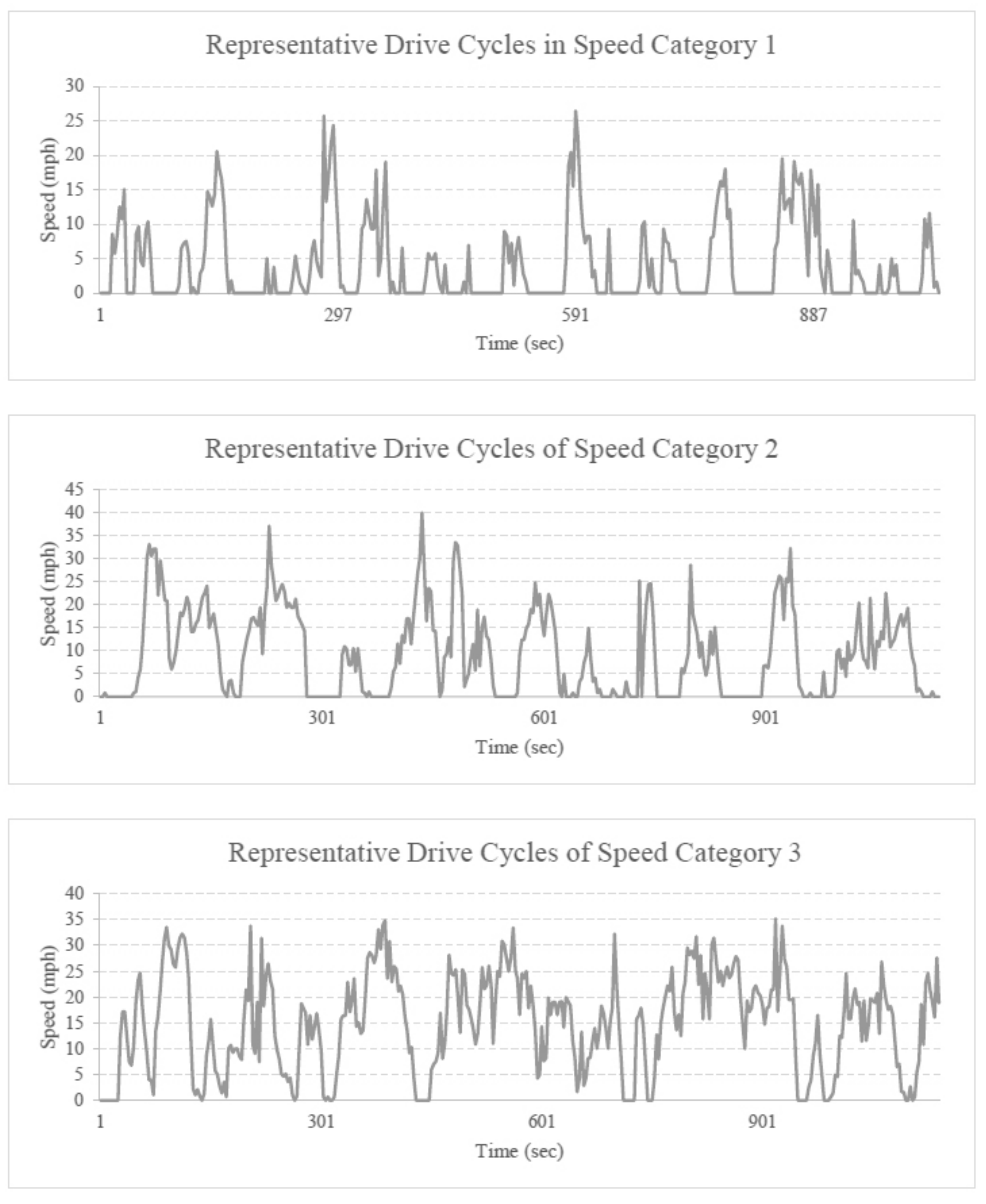
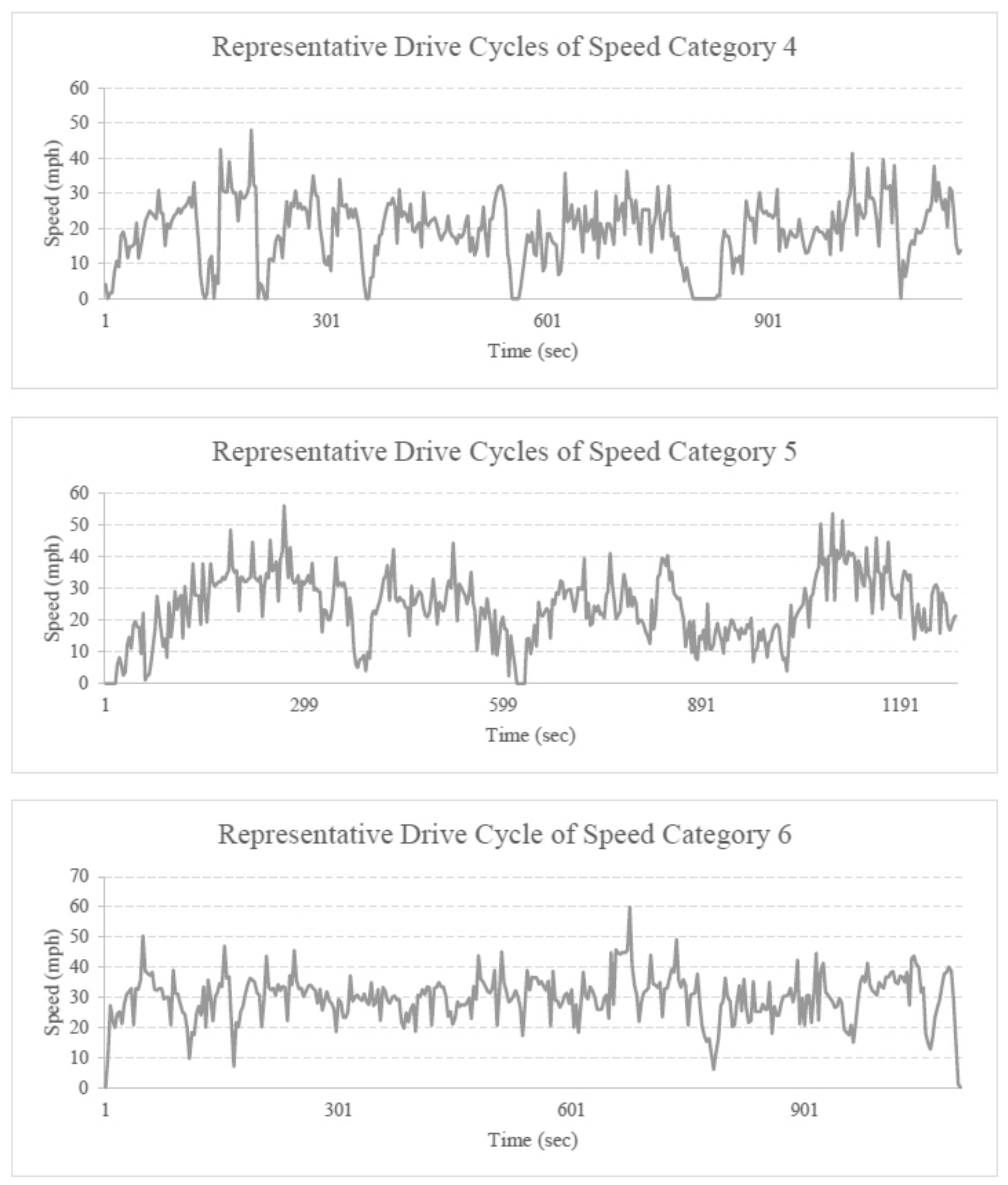
4.2.3. Drive Cycle Validation

The target operating mode distribution arrays and representative drive cycles of each group have been developed by the selection-to-rebuild process. At this stage, a total of 48 representative drive cycles is generated and classified considering the combination of six-speed categories, four time-of-day and two day-of-week. The validity of the classification and the drive cycles need to be tested. A horizontal experiment is required to see if the drive cycles from the same speed category but different time-of-day or day-of-week attributes are truly different. A vertical comparison is also required to validate the representativeness of the developed drive cycles with the data from the control group. Same as the drive cycle developing process, the square root of the SSR with maximum acceptance at 0.05 is used as the indicator. The overall validation process consists of the following three tests:

• The comparison of drive cycles from same speed category and time-of-day but in different day-of-week.
• The comparison of drive cycles from same speed category and day-of-week but in different time-of-day.
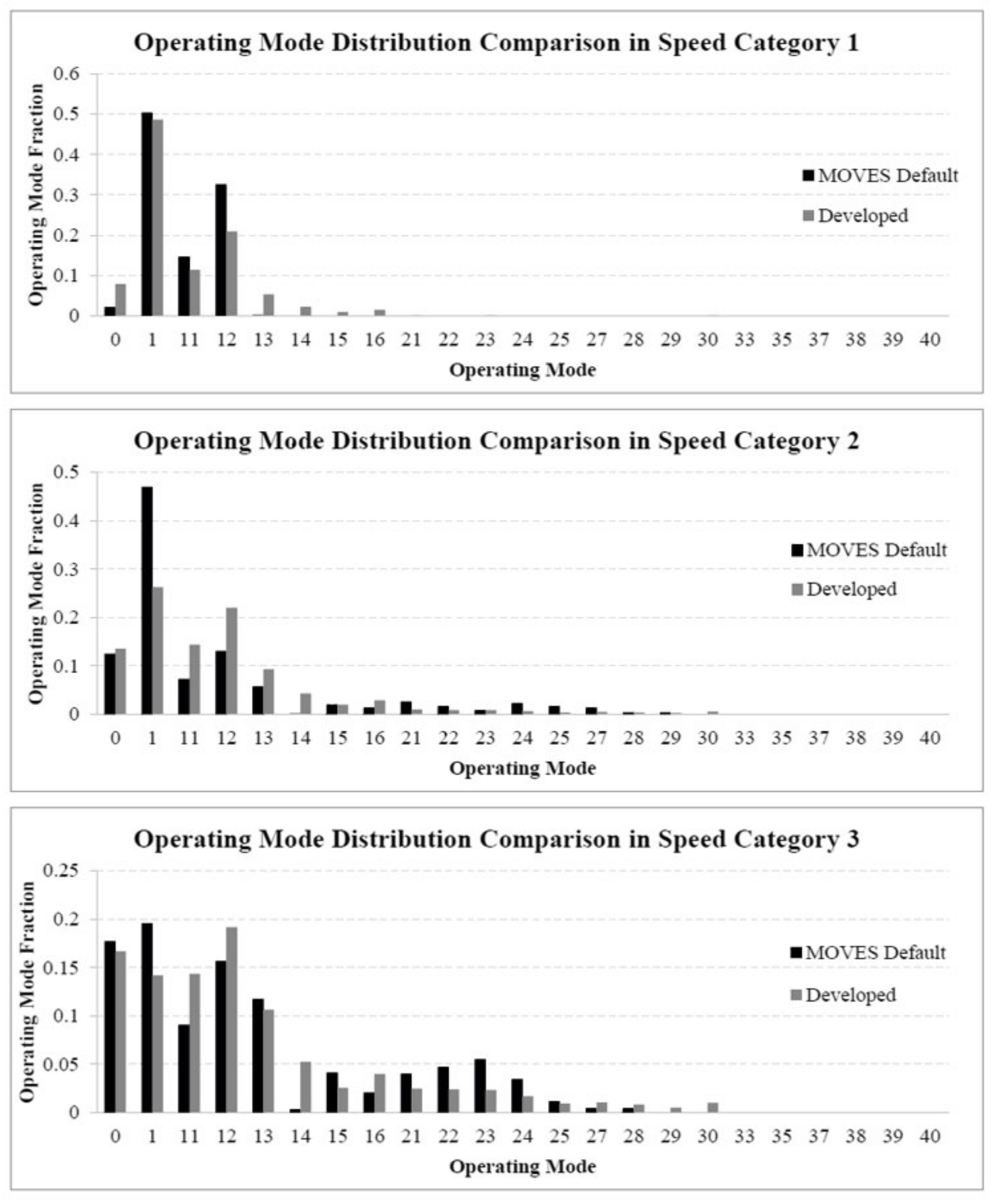
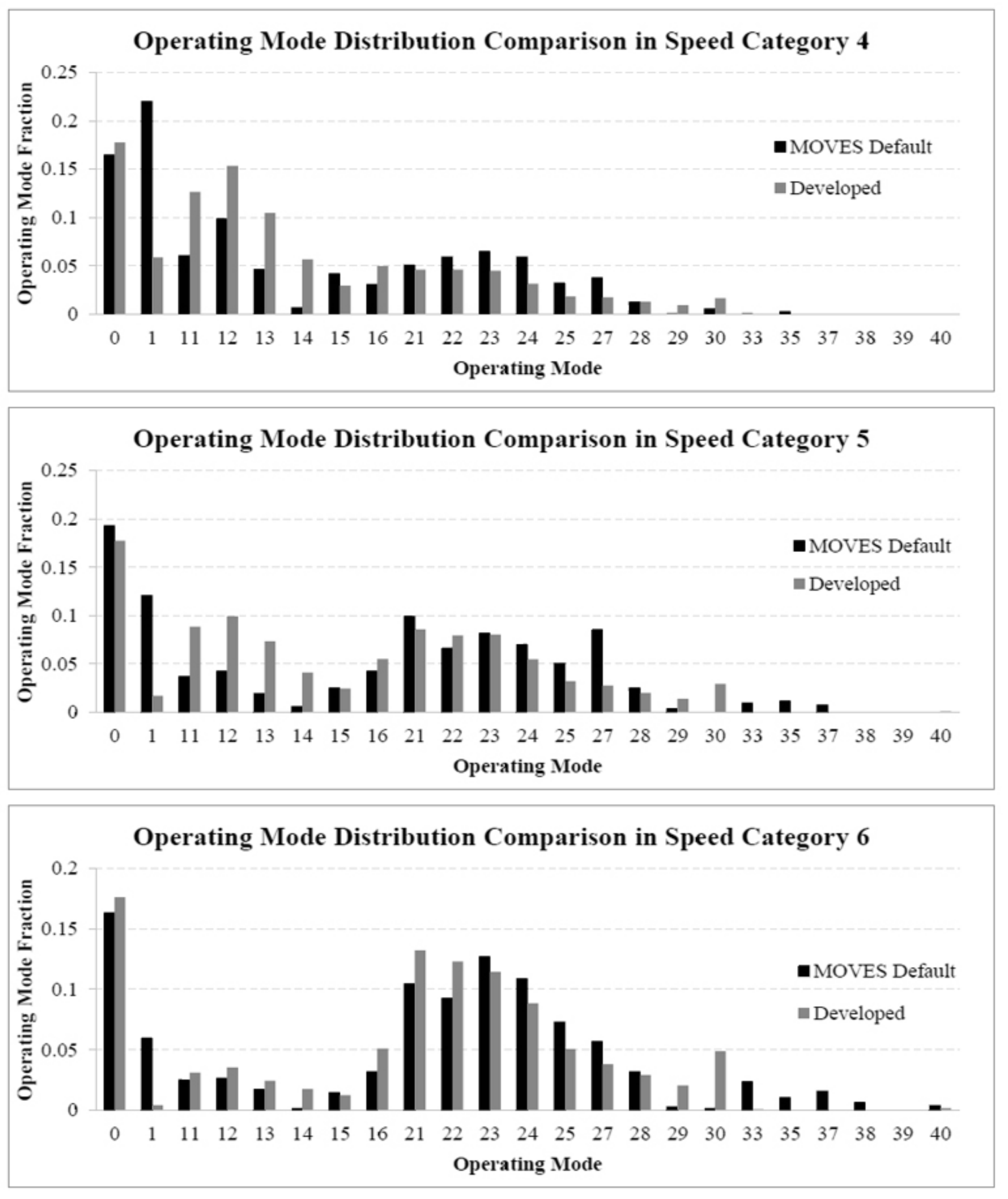
• The comparison in operating mode distributions between the representative drive cycles with the target operating mode distribution from the control group in each classification.

5. Discussion

5.1. Validation of Developed Drive Cycles with Selected Criteria

The drive cycle validation process is to compare the operating mode distribution of the developed drive cycle with the target distribution from the control group (data from the fourth week) in the same speed category under the same data processing procedure. The difference between the operating mode distributions of all cases in weekdays is listed in

Table 4. Differences in operating mode distributions for drive cycle validation (C_developed − C_control).

Speed Category	AM Peak	Midday	PM Peak	Overnight
1	0.045	0.022	0.047	0.023
2	0.014	0.013	0.058	0.041
3	0.023	0.022	0.049	0.043
4	0.053	0.013	0.036	0.042
5	0.030	0.013	0.051	0.014
6	0.038	0.051	0.046	0.017

. Almost all the cases have the values of their indicators at less than or close to 0.05. In other words, the drive cycles developed from three-week data can represent the driving patterns in the same category of the fourth week. In other words, the drive cycles developed under this methodology are valid and general to represent local driving patterns during weekdays in the study area.

5.2. Drive Cycle Summary and Comparison with the MOVES Default Drive Cycles

The drive cycles developed from this study were categorized by the different time-periods of the day, different day of the week and the speed categories used by the MOVES default drive cycles. Figure 1 shows a sample of the constructed weekday representative drive cycles in the format of a speed vs. timeline chart. Furthermore, these drive cycles are compared with the MOVES default drive cycles within the same speed category.

Table 5. Basic statistics between the developed drive cycles and the MOVES default drive cycles in the same speed category.

Speed Category	Drive Cycle Description	Duration (sec)	Distance (mile)	Maximum Speed (mph)	Average Speed (mph)	Maximum Acceleration (mph/s)	Maximum Deceleration (mph/s)	Idle Percentage (%)	Difference in Operating Mode Distribution
1	MOVES	602	0.4	10	2.5	2.4	−2.5	50.3	0.147
	Developed	1044	1.2	26.4	3.9	7.8	−5.1	48.6
2	MOVES	853	2.1	44.2	8.7	5.1	−5	46.9	0.245
	Developed	1.135	2.9	40.0	9.2	6.9	−8.4	26.2
3	MOVES	870	3.8	37.9	15.7	4.8	−5.4	19.5	0.111
	Developed	1141	4.7	35.2	14.9	7.9	−7.6	14.2
4	MOVES	709	3.7	50.3	18.6	5.8	−8.2	22.0	0.205
	Developed	1162	6.2	48.1	19.3	7.0	−6.3	5.9
5	MOVES	513	3.6	53.1	25.4	5.5	−7.5	12.1	0.163
	Developed	1273	8.6	56.2	24.1	6.4	−9.1	1.7
6	MOVES	754	6.5	63.8	31.0	5.7	−5.8	6.0	0.103
	Developed	1102	9.2	59.9	29.8	7.3	−7.4	0.4

summarizes the basic statistics between the developed drive cycles and the MOVES default drive cycles from speed category 1 to category 6, due to the same categorizing definitions. The differences were identified with the parameters such as distance, maximum speed, maximum acceleration/deceleration, average speed, idle percentages and operating mode distributions. Although the average speeds between the cycles are similar, differences in operating mode distributions suggest that the local drive cycles have significantly different driving patterns compared to the MOVES default drive cycles by comparing the operating mode distribution as expected. The difference in idle percentage is another indicator to support the variances. Figure 2 visualizes the differences in operating mode distributions as a set of column charts. It is clear from the figures that the MOVES model’s default drive cycles heavily overestimate the proportion of idling operating mode (Bin 1) by 1.7%, 20.7%, 5%, 14.1%, 11.4% and 6% from speed category 1 to speed category 6, respectively. In speed categories 5 and 6, there are notable proportions of high-speed operating modes (Bin 33, Bin 35 and Bin37) in the MOVES drive cycles. However, such operating mode fractions in local drive cycles are negligible. In contrast, the localized drive cycles show a much more concentrated proportion in the low-speed cruising operating modes (Bin 11 to Bin 14) and a lower upper limit in the speed values. All these variances tell of the significantly different driving patterns between the study area and the MOVES model default environment.

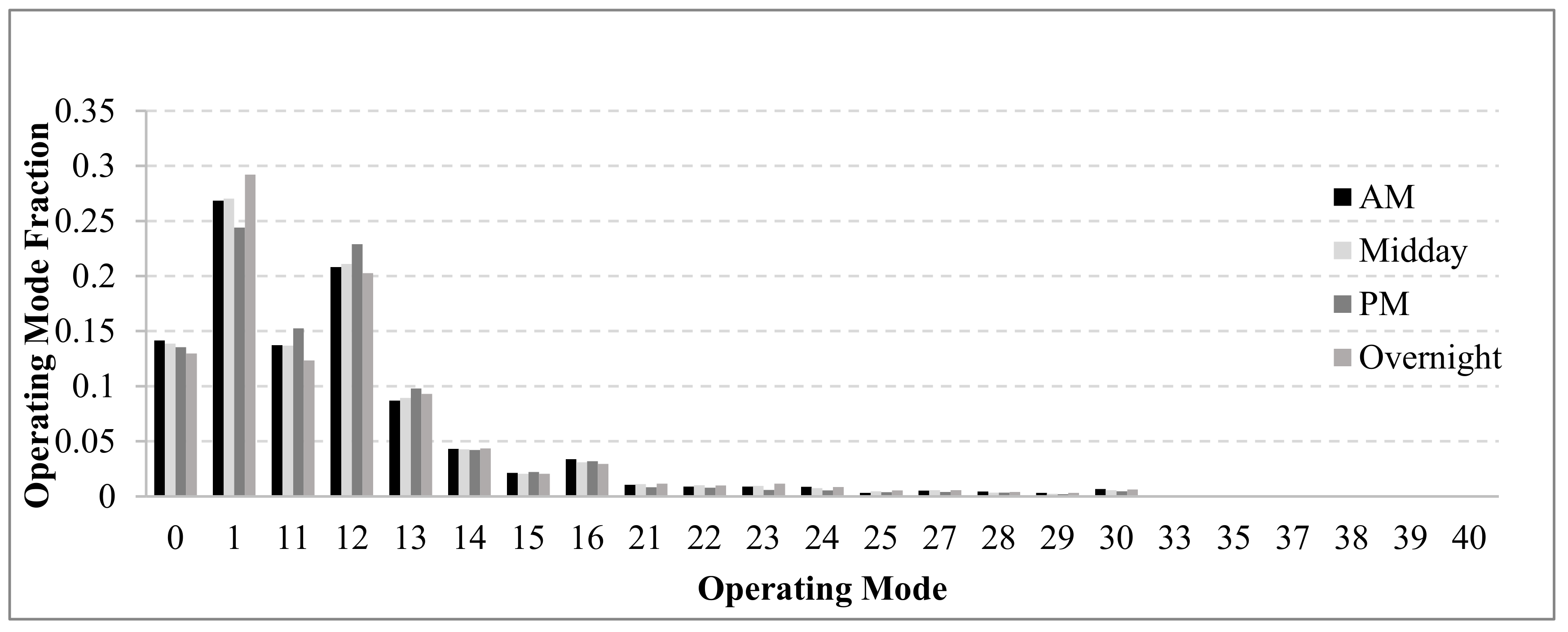
5.3. Sensitivity of Time-of-Day

Each two drive cycles of the four time-of-day categories with the same speed and day-of-week attribute were compared in operating mode distributions. The results in Table 4 that have values less than 0.05 could be considered as having no significant variance between the drive cycles by the same definition of the drive cycle building criteria. Based on the results from

Table 6. Differences in the operating mode distributions for the sensitivity analysis of time-of-day.

Day of Week	Speed Category	${\mathit{C}}_{\mathit{A}\mathit{M}}-{\mathit{C}}_{\mathit{M}\mathit{D}}$	${\mathit{C}}_{\mathit{A}\mathit{M}}-{\mathit{C}}_{\mathit{P}\mathit{M}}$	${\mathit{C}}_{\mathit{A}\mathit{M}}-{\mathit{C}}_{\mathit{O}\mathit{N}}$	${\mathit{C}}_{\mathit{P}\mathit{M}}-{\mathit{C}}_{\mathit{M}\mathit{D}}$	${\mathit{C}}_{\mathit{O}\mathit{N}}-{\mathit{C}}_{\mathit{M}\mathit{D}}$	${\mathit{C}}_{\mathit{O}\mathit{N}}-{\mathit{C}}_{\mathit{P}\mathit{M}}$
Weekday	1	0.018	0.045	0.046	0.031	0.061	0.071
	2	0.006	0.038	0.031	0.037	0.029	0.067
	3	0.014	0.043	0.034	0.039	0.033	0.065
	4	0.024	0.033	0.030	0.035	0.025	0.055
	5	0.034	0.047	0.026	0.016	0.031	0.033
	6	0.028	0.054	0.042	0.029	0.025	0.037
Weekend	1	0.050	0.051	0.033	0.018	0.022	0.044
	2	0.055	0.057	0.055	0.033	0.014	0.037
	3	0.035	0.063	0.026	0.028	0.024	0.047
	4	0.071	0.061	0.039	0.024	0.049	0.071
	5	0.041	0.039	0.029	0.021	0.030	0.028
	6	0.048	0.049	0.046	0.030	0.053	0.047

, it is clear from the table that the general driving patterns of a trip with a low average speed, less than or equal to 20 mph (speed category 4), between overnight and PM during weekdays, might be slightly different in the study area. In addition, during weekends, the trips with a low average speed (below speed category 4) between AM and PM are having variances based on the criteria. All the other combinations show that the differences between the operating mode distributions are not sensitive to the selected time-of-day period. By analyzing the operating mode distributions, it is found that the differences are mainly coming from the discrepancy between the fractions of the idle operating mode (Bin 1) and the low speed cruising operating mode (Bin 12). In other words, it indicates that the vehicle trips which have a low average speed in the weekday PM peak hours are due to longer idling time and the same group of vehicles in a weekday overnight are due to a longer cruising time, and so do the differences between the weekend AM period and PM period. This finding appears to be grounded in common sense, in that the traffic demand is significantly lower during weekday overnight and weekend AM than it is in both PM periods. Figure 3 shows the difference with the example of the operating mode distributions of weekday drive cycles in speed category 2.

6. Conclusions

This paper presented a drive cycle developing case study using anonymized GPS route data from rideshare vehicles in Chengdu, China. A data-filtering procedure based on acceleration and vehicle specific power thresholds was established to process the GPS data. A micro-trip selection-to-rebuild method with operating mode distribution was used to develop a series of average-speed categorized representative drive cycles. The speed categorized drive cycles passed the representativeness test. The sensitivities of the time-of-day and day-of-week were examined for the drive cycles. The results showed that the day-of-week is insensitive to the speed categories. The time-of-day is insensitive to the drive cycles among most cases, except for the driving patterns of a trip with a low average speed (less than 20 mph) between the overnight and PM period on weekdays and between the AM period and PM period on weekends. Overall, a series of weekday daily average drive cycles were finalized and compared to the MOVES default drive cycles that are built with a similar strategy. The results showed that MOVES default drive cycles heavily overestimate the proportion of the idling operating mode (Bin 1). In speed categories 5 and 6, there are notable proportions of high-speed operating modes (Bin 33, Bin 35 and Bin37) in the MOVES drive cycles. However, such operating mode fractions in the local drive cycles are negligible. In contrast, the local drive cycles show a much more concentrated proportion of low-speed cruising operating modes (Bin 11 to Bin 14) and a lower upper limit in speed values. All these variances tell of the significantly different driving patterns between the study area and MOVES default environment. The results support the importance of developing local drive cycles to capture regional driving activity patterns.

On the other hand, the results generated by using such a novel dataset with an algorithm for emission modeling, MOVES in this study, can achieve much more. The study showed the capability of using this uninterrupted, anonymous mega data set to create a localized drive cycle database to improve the accuracy of the emission estimates. With big-data processing tools, a larger drive cycle database can be established for any city where rideshare service is provided, and further categorization of their drive cycles, such as speed and time-of-day, are able to be achieved and statistically valid by using big data instead of traditional small CC or IV datasets. Comparisons with other drive cycles developed by rideshare and passenger cars in different cities with similar speed categories will be a very good indicator of the driving patterns around the country. To accomplish these goals, studies still need to be conducted to further address the general problems in GPS datasets, such as accuracy of observation, speed and acceleration lags with a better data recovering algorithm and more information about the vehicles. Additionally, more data from different seasons, different years and larger geographical coverage will help further validate the drive cycles developed in this study area.

References

1. Wang, S.; Hao, J. Air quality management in China: Issues, challenges, and options. J. Environ. Sci. 2012, 24, 2–13. [Google Scholar] [CrossRef]
2. Zhang, L.; Jacob, D.J.; Boersma, K.F.; Jaffe, D.A.; Olson, J.R.; Bowman, K.W.; Worden, J.R.; Thompson, A.M.; Avery, M.A.; Cohen, R.C.; et al. Transpacific transport of ozone pollution and the effect of recent Asian emission increases on air quality in North America: An integrated analysis using satellite, aircraft, ozonesonde, and surface observations. Atmos. Chem. Phys. Discuss. 2008, 8, 8143–8191. [Google Scholar]
3. Facanha, C.; Horvath, A. Evaluation of life-cycle air emission factors of freight transportation. Environ. Sci. Technol. 2007, 41, 7138–7144. [Google Scholar] [CrossRef] [PubMed]
4. Alessandrini, A.; Orecchini, F. A driving cycle for electrically-driven vehicles in Rome. Proc. Inst. Mech. Eng. Part D J. Automob. Eng. 2003, 217, 781–789. [Google Scholar] [CrossRef]
5. Esteves-Booth, A.; Muneer, T.; Kubie, J.; Kirby, H. A review of vehicular emission models and driving cycles. Proc. Inst. Mech. Eng. Part C J. Mech. Eng. Sci. 2002, 216, 777–797. [Google Scholar] [CrossRef]
6. Weiss, M.; Bonnel, P.; Hummel, R.; Manfredi, U.; Colombo, R.; Lanappe, G.; Le Lijour, P.; Sculati, M. Analyzing on-road emissions of light-duty vehicles with Portable Emission Measurement Systems (PEMS). JRC Sci. Techn. Rep. EUR 2011, 24697. Available online: http://citeseerx.ist.psu.edu/viewdoc/download?doi=10.1.1.204.5287&rep=rep1&type=pdf (accessed on 20 October 2020).
7. Papson, A.; Hartley, S.; Kuo, K.-L. Analysis of emissions at congested and uncongested intersections with motor vehicle emission simulation 2010. Transp. Res. Rec. 2012, 2270, 124–131. [Google Scholar] [CrossRef]
8. Montazeri-Gh, M.; Naghizadeh, M. Development of car drive cycle for simulation of emissions and fuel economy. In Proceedings of the 15th European Simulation Symposium, Delft, The Netherlands, 26–29 October 2003. [Google Scholar]
9. Cai, H.; Jia, X.; Chiu, A.S.F.; Hu, X.; Xu, M. Siting public electric vehicle charging stations in Beijing using big-data informed travel patterns of the taxi fleet. Transp. Res. Part D Transp. Environ. 2014, 33, 39–46. [Google Scholar] [CrossRef] [Green Version]
10. Li, W.; Pu, Z.; Li, Y.; Ban, X. Characterization of Ridesplitting Based on Observed Data: A Case Study of Chengdu, China. Transp. Res. Part C Emerg. Technol. 2019, 100, 330–353. [Google Scholar] [CrossRef]
11. Wang, H.; Chen, C.; Huang, C.; Fu, L. On-road vehicle emission inventory and its uncertainty analysis for Shanghai, China. Sci. Total Environ. 2018, 398, 60–67. [Google Scholar] [CrossRef] [PubMed]
12. GAIA Open Dataset. Available online: https://outreach.didichuxing.com/research/opendata/en/ (accessed on 21 January 2021).
13. Yu, L.; Wang, Z.; Shi, Q. PEMS-Based Approach to Developing and Evaluating Driving Cycles for Air Quality Assessment; Texas Southern University: Houston, TX, USA, 2010. [Google Scholar]
14. Tzirakis, E.; Pitsas, K.; Zannikos, F.; Stournas, S. Vehicle emissions and driving cycles: Comparison of the Athens driving cycle (ADC) with ECE-15 and European driving cycle (EDC). Glob. NEST J. 2006, 8, 282–290. [Google Scholar]
15. Technical Standard for 10.15-Mode Exhaust Emission Measurement for Gasoline-Fueled Motor Vehiclesle. Available online: https://www.epa.gov/vehicle-and-fuel-emissions-testing/dynamometer-drive-schedules#japanese (accessed on 21 January 2021).
16. Austin, T.C.; DiGenova, F.J.; Carlson, T.R.; Joy, R.W.; Gianolini, K.A. Characterization of Driving Patterns and Emissions from Light-Duty Vehicles in California; Final Report. No. PB-94-157005/XAB; Sierra Research, Inc.: Sacramento, CA, USA, 1993. [Google Scholar]
17. Farzaneh, M.; Zietsman, J.A.; Lee, D.; Johnson, J.; Wood, N.; Ramani, T.; Gu, C. Texas-Specific Drive Cycles and Idle Emissions Rates for Using with EPA’s MOVES Model—Final Report; Texas Department of Transportation: Austin, TX, USA, 2014. [Google Scholar]
18. Pu, Z.; Zhu, M.; Li, W.; Cui, Z.; Guo, X.; Wang, Y. Monitoring Public Transit Ridership Flow by Passively Sensing Wi-Fi and Bluetooth Mobile Devices. IEEE Internet Things J. 2021, 8, 474–486. [Google Scholar] [CrossRef]
19. Carlson, T.R.; Austin, R.C. Development of Speed Correction Cycles; Report SR97-04-01; Sierra Research Inc.: Sacramento, CA, USA, 1996. [Google Scholar]
20. Morey, J.E.; Limanond, T.; Niemeier, D.A. Validity of chase car data used in developing emissions cycles. Stat. Anaysis Model. Automot. Emiss. 2001, 3, 15–28. [Google Scholar]
21. Niemeier, D.A.; Limanond, T.; Morey, J.E. Data Collection for Driving Cycle Development: Evaluation of Data Collection Protocols; Institute of Transportation Studies, University of California at Davis: Davis, CA, USA, 1999. [Google Scholar]
22. Jackson, E.; Aultman-Hall, L.; Holmén, B.A.; Du, J. Evaluating the ability of global positioning system receivers to measure a real-world operating mode for emissions research. Transp. Res. Rec. 2005, 1941, 43–50. [Google Scholar] [CrossRef]
23. Wang, Q.; Huo, H.; He, K.; Yao, Z.; Zhang, Q. Characterization of vehicle driving patterns and development of driving cycles in Chinese cities. Transp. Res. Part D Transp. Environ. 2008, 13, 289–297. [Google Scholar] [CrossRef]
24. Wang, H.; Zhang, X.; Ouyang, M. Energy consumption of electric vehicles based on real-world driving patterns: A case study of Beijing. Appl. Energy 2015, 157, 710–719. [Google Scholar] [CrossRef]
25. Eastern Research Group. Roadway-Specific Driving Schedules for Heavy-Duty Vehicle; Prepared for EPA; Eastern Research Group: Lexington, MA, USA, 2003. [Google Scholar]
Figure 1. Weekday representative drive cycles of each speed category.
Sustainability 13 02114 g001aSustainability 13 02114 g001b
Figure 2. Comparison between the developed drive cycles and the MOVES default drive cycles in operating mode distribution.
Sustainability 13 02114 g002aSustainability 13 02114 g002b
Figure 3. Operating mode distributions of weekday drive cycles by time-of-day in speed category 2.
Sustainability 13 02114 g003