
Evaluating Operational Features of Three Unconventional Intersections under Heavy Traffic Based on CRITIC Method


Abstract
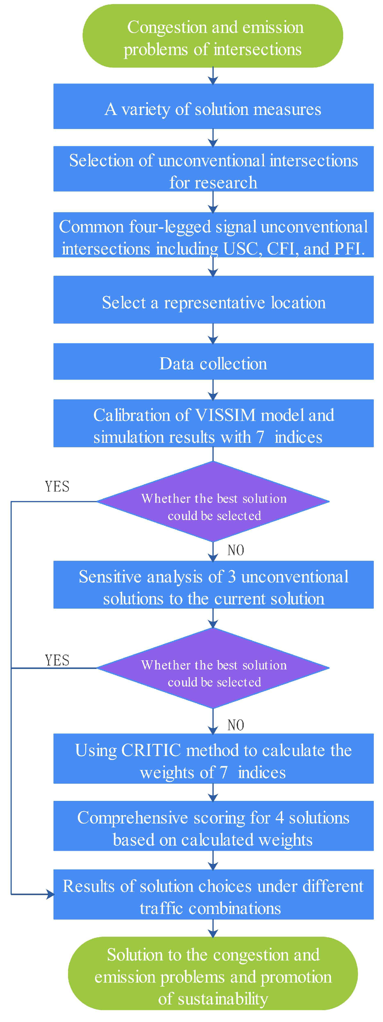
:1. Introduction
2. Problem Statement and Data Collection
2.1. Problem Statement
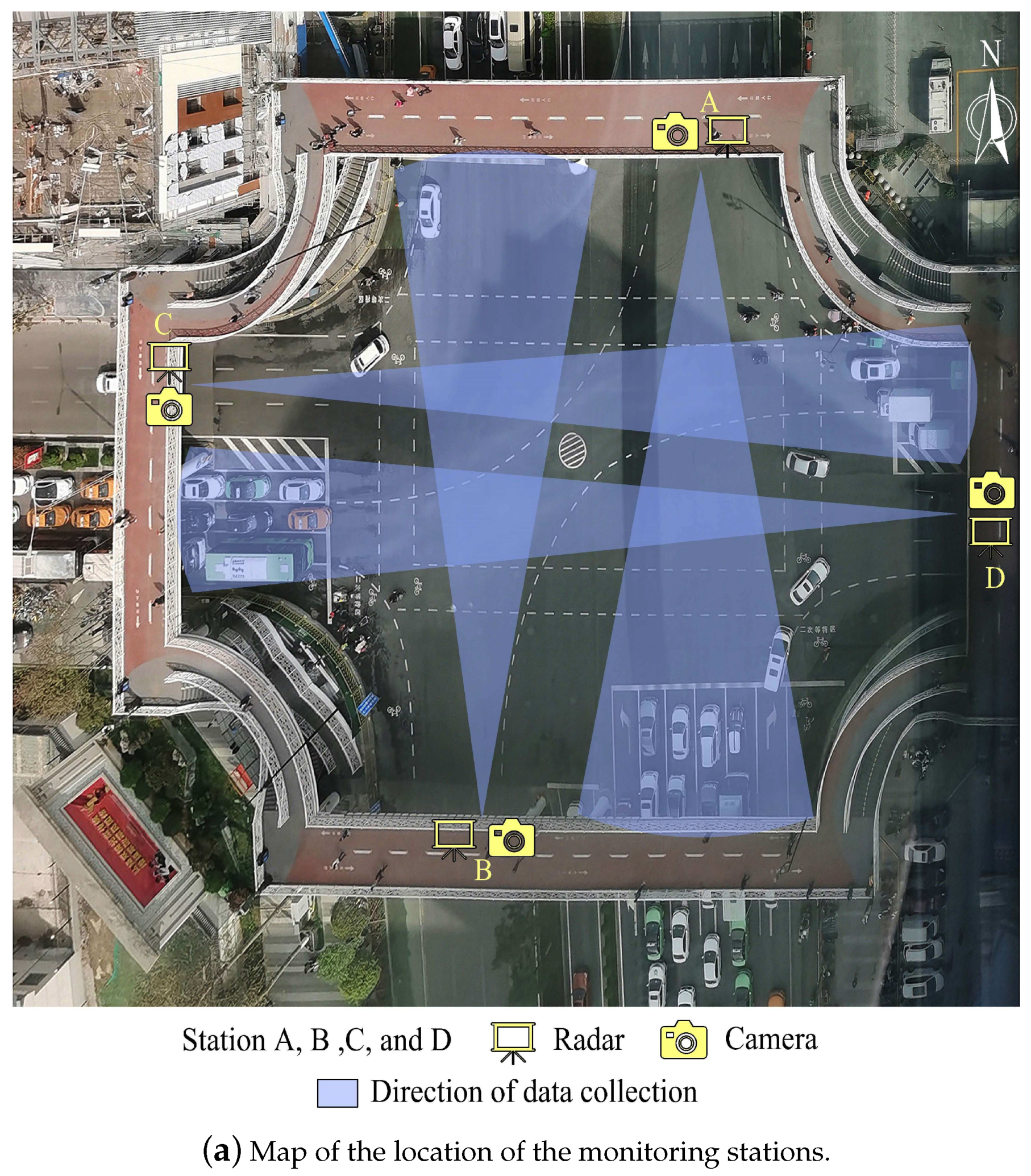
2.2. Data Collection
- The two intersecting roads at the intersection had obvious primary and secondary characteristics, where the north–south direction was the main road, the east–west direction was the secondary road, and the traffic volume in the north–south direction was higher than the traffic volume in the east–west direction.
- The total traffic volumes at the intersection were nearly the same for northbound and southbound, and nearly the same for eastbound and westbound.
- The proportion of left-turning vehicles at the intersection was nearly the same for northbound and southbound (14.78% and 12.63%, respectively), and the proportion of left-turning traffic was relatively close for eastbound and westbound (13.58% and 20.69%, respectively).
- The proportion of vehicles making a U-turn was not large.
- The maximum speed of vehicles approached 70 km/h, while the average speed was only about 20 km/h, meaning that most of the vehicles were not moving fast.
- The signal cycle was 175 s, and the split times were the same for southbound and northbound; the westbound straight and left-turn phases started and ended at the same time, while the eastbound straight phase started first, the left-turn phase started later and, finally, the straight and left-turn phases ended at the same time. It is worth noting that there was a period of time when the green light was on simultaneously for westbound left-turning vehicles and eastbound straight-through vehicles, which indicates a conflict point between left-turning and straight-through vehicles.
- There was a waiting area at the intersection. The northbound and southbound left-turn waiting area contained three lanes, while the eastbound and westbound left-turn waiting area contained two lanes.
- In 2020, the proportion of new-energy vehicle was 2.83% in Xi’an [78]. Therefore, the vehicles studied in this paper were traditional vehicles only.
3. Establishment and Simulation of the Model in VISSIM
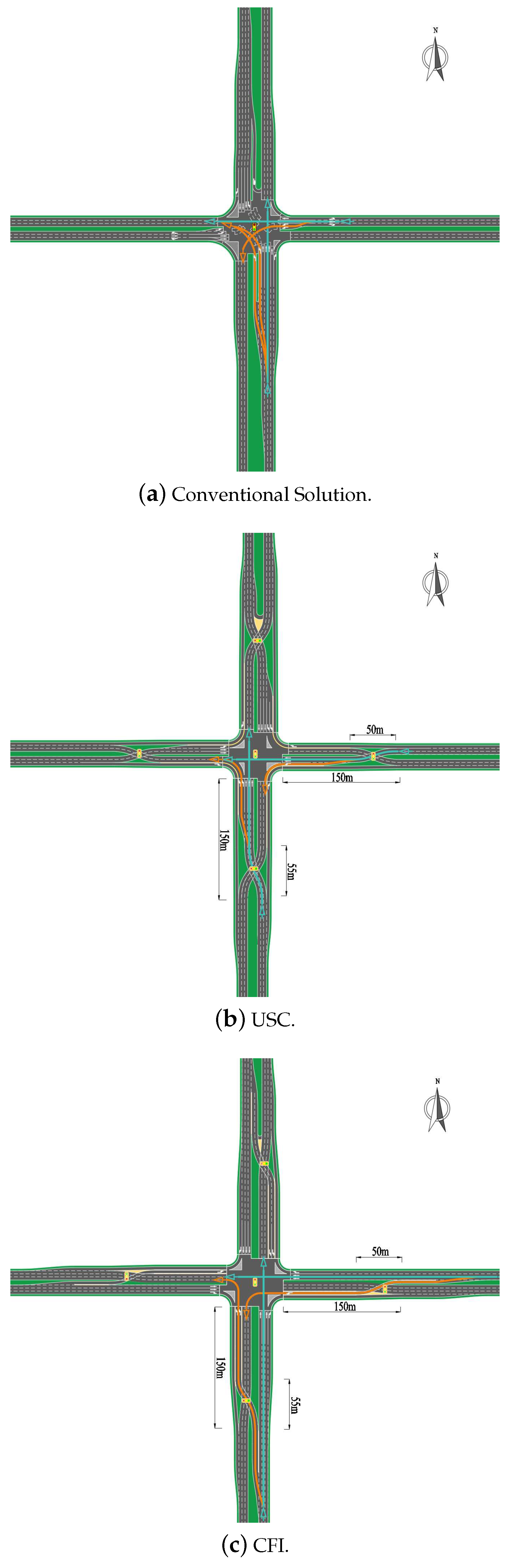
3.1. Modeling of Each Solution
3.1.1. Geometric Design
3.1.2. Signal Phasing and Timing
3.2. Calibration of Vissim Model
- First, the capacity of each flow needs to be determined, which can be calculated by (1):where C denotes the ideal capacity (veh/h) and denotes the average minimum headway(s).
- The MAPE index represents the mean absolute percentage error, which is used to reflect the error between the actual collected and simulated capacity of each flow. The MAPE can be calculated according to (2):where a denotes the traffic flow, n denotes a total of 13 different traffic flows, is the simulated capacity of VISSIM (veh/h), and denotes the collected capacity (veh/h). Table 2 shows the calculated MAPE results for each traffic flow.
3.3. VISSIM Calculation of Operational Measures
3.3.1. Selection of Evaluation Indices
3.3.2. Simulation Results
3.4. Safety Evaluation
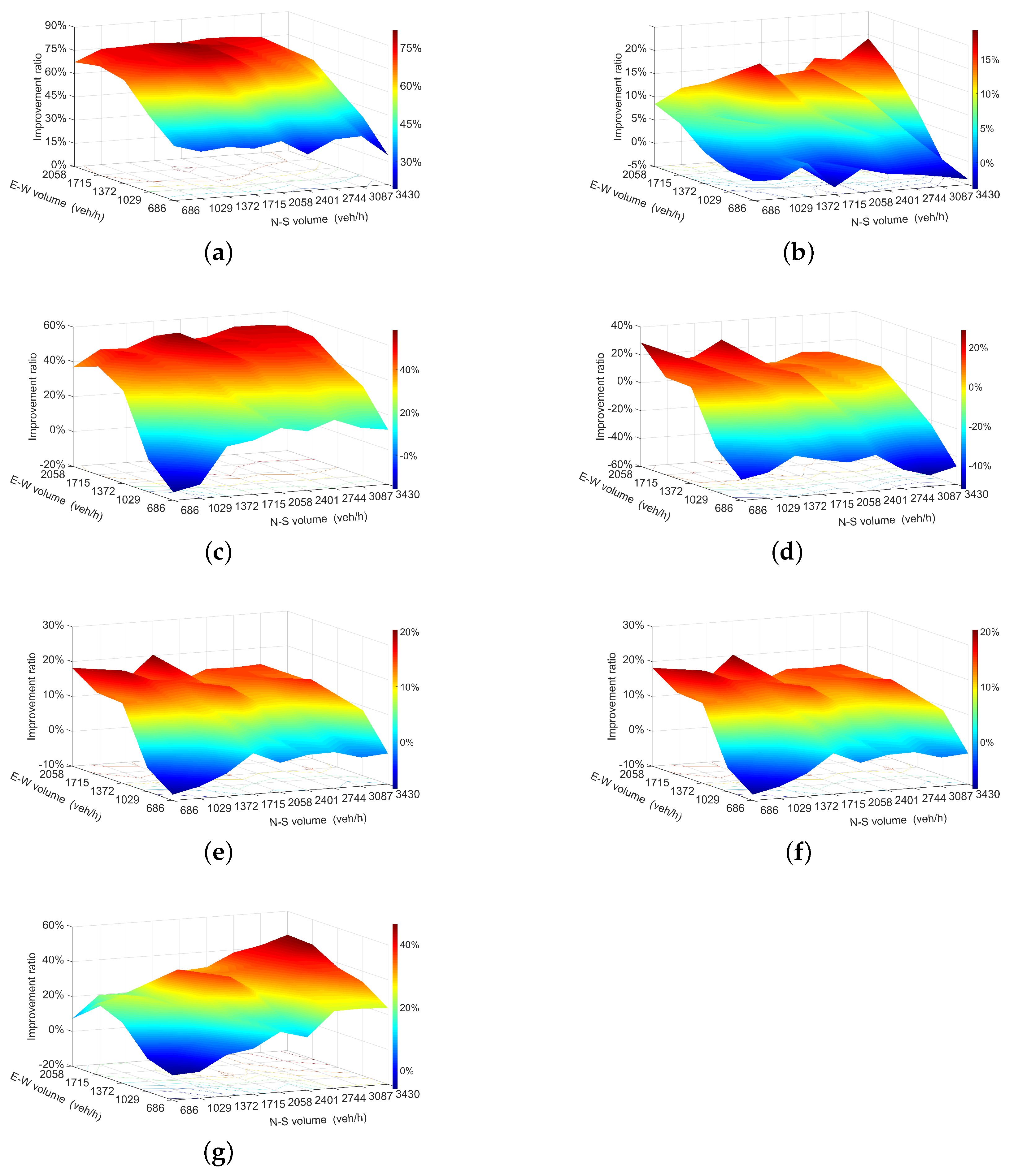
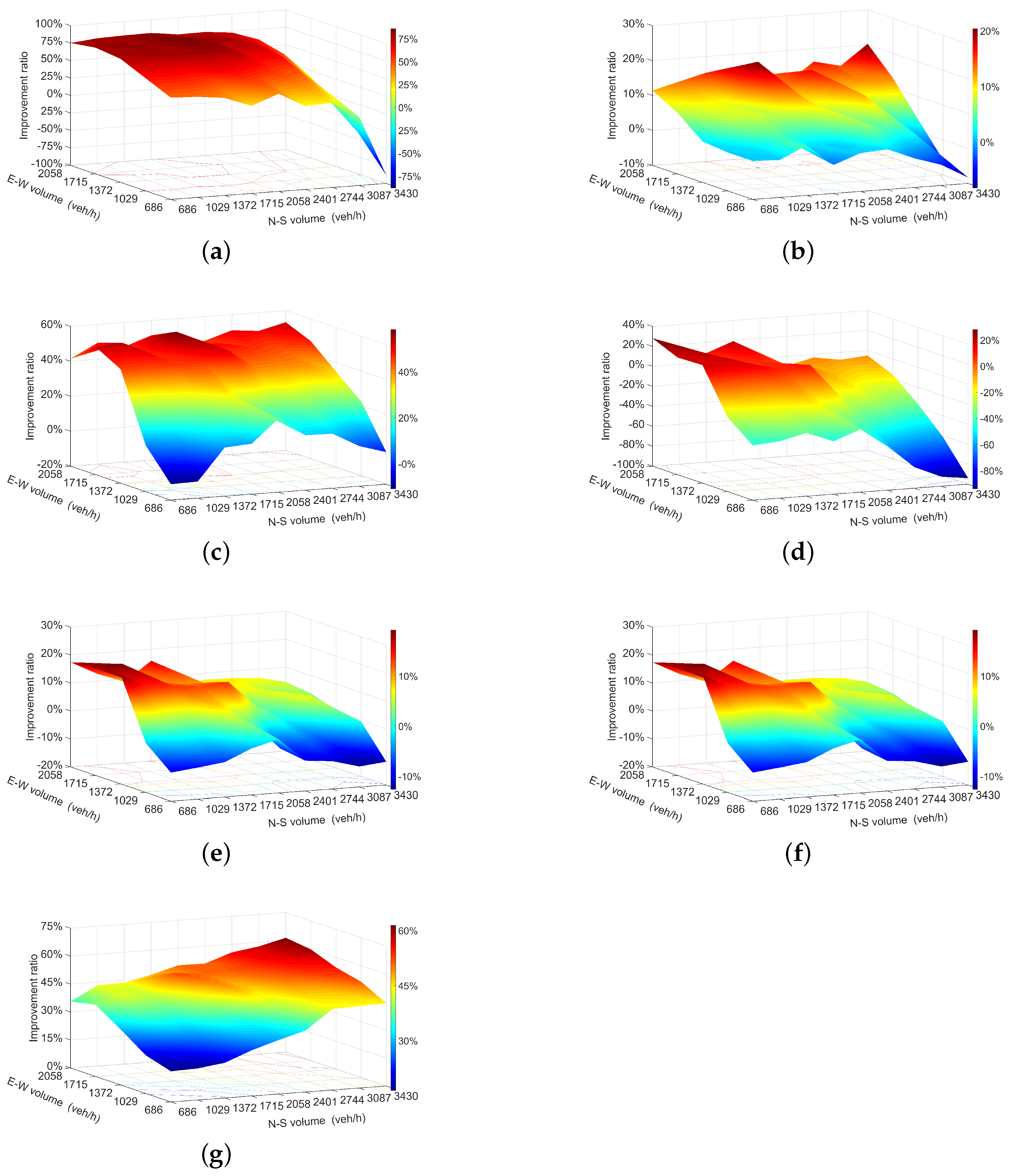
4. Sensitivity Analysis of Operational Performance
5. Analysis of the Results Based on the Critic Method
5.1. Calculation of Weighting of Indices
5.2. Evaluation of Solutions
6. Conclusions
Author Contributions
Funding
Acknowledgments
Conflicts of Interest
References
- Al-Dabbagh, M.S.M.; Al-Sherbaz, A.; Turner, S. The impact of road intersection topology on traffic congestion in urban cities. In Intelligent Systems and Applications, IntelliSys 2018, Advances in Intelligent Systems and Computing; Arai, K., Kapoor, S., Bhatia, R., Eds.; Springer: Cham, Switzerland, 2018; Volume 868. [Google Scholar]
- Stevanovic, A.; Mitrovic, N. Traffic microsimulation for flexible utilization of urban roadways. Transp. Res. Rec. J. Transp. Res. Board 2019, 2673, 92–104. [Google Scholar] [CrossRef]
- Wang, H.; Luo, S.; Luo, T. Fractal characteristics of urban surface transit and road networks: Case study of Strasbourg, France. Adv. Mech. Eng. 2017, 9. [Google Scholar] [CrossRef] [Green Version]
- Ma, M.; Yang, Q.; Liang, S.; Wang, Y. A new coordinated control method on the intersection of traffic region. Discret. Dyn. Nat. Soc. Hindawi 2016, 2016, 1–10. [Google Scholar] [CrossRef] [Green Version]
- Li, S.; Li, G.; Cheng, Y.; Ran, B. Intersection congestion analysis based on cellular activity data. IEEE Access 2020, 8, 43476–43481. [Google Scholar] [CrossRef]
- Chen, K.; Zhao, J.; Knoop, V.L.; Gao, X. Robust signal control of exit lanes for left-turn intersections with the consideration of traffic fluctuation. IEEE Access 2020, 8, 42071–42081. [Google Scholar] [CrossRef]
- Sun, X.; Lin, K.; Jiao, P.; Lu, H. The dynamical decision model of intersection congestion based on risk identification. Sustainability 2020, 12, 5923. [Google Scholar] [CrossRef]
- Astarita, V.; Caliendo, C.; Giofrè, V.P.; Russo, I. Surrogate safety measures from traffic simulation: Validation of safety indicators with intersection traffic crash data. Sustainability 2020, 12, 6974. [Google Scholar] [CrossRef]
- Chen, J.; Wang, W.; Li, Z. Dispersion effect in left-turning bicycle traffic and its influence on capacity of left-turning vehicles at signalized intersections. Transp. Res. Rec. J. Transp. Res. Board 2014, 2468, 38–46. [Google Scholar] [CrossRef]
- Zhang, H.; Jiang, R.; Hu, M.; Jia, B. Analytical investigation on the minimum traffic delay at a three-phase signalized t-type intersection. Mod. Phys. Lett. B 2017, 31, 1–9. [Google Scholar] [CrossRef]
- Yan, Y.; Qu, X.; Li, H. On the design and operational performance of waiting areas in at-grade signalized intersections: An overview. Transp. A Transp. Sci. 2018, 14, 901–928. [Google Scholar] [CrossRef]
- Yang, Q.; Shi, Z. Effects of the design of waiting areas on the dynamic behavior of queues at signalized intersections. Phys. A Stat. Mech. Appl. 2018, 509, 181–195. [Google Scholar] [CrossRef]
- Hao, W.; Ma, C.; Moghimi, B.; Fan, Y.; Gao, Z. Robust optimization of signal control parameters for unsaturated intersection based on tabu search-artificial bee colony algorithm. IEEE Access 2018, 6, 32015–32022. [Google Scholar] [CrossRef]
- Hao, W.; Lin, Y.; Cheng, Y.; Yang, X. Signal progression model for long arterial: Intersection grouping and coordination. IEEE Access 2018, 6, 30128–30136. [Google Scholar] [CrossRef]
- Li, J.; Wang, W.; Zuylen, H.J.; Sze, N.N.; Chen, X.; Wang, H. Predictive Strategy for Transit Signal Priority at Fixed-Time Signalized Intersections: Case Study in Nanjing, China. Transp. Res. Record 2012, 2311, 124–131. [Google Scholar] [CrossRef]
- Cruz-Piris, L.; Lopez-Carmona, M.A.; Marsa-Maestre, I. Automated optimization of intersections using a genetic algorithm. IEEE Access 2019, 7, 15452–15468. [Google Scholar] [CrossRef]
- Małecki, K. The Importance of Automatic Traffic Lights time Algorithms to Reduce the Negative Impact of Transport on the Urban Environment. Transp. Res. Procedia 2016, 16, 329–342. [Google Scholar]
- Jia, H.; Lin, Y.; Luo, Q.; Li, Y.; Miao, H. Multi-objective optimization of urban road intersection signal timing based on particle swarm optimization algorithm. Adv. Mech. Eng. 2019, 11. [Google Scholar] [CrossRef] [Green Version]
- Małecki, K.; Pietruszka, P. Comparative Analysis of Chosen Adaptive Traffic Control Algorithms. Recent Adv. Traffic Eng. Transp. Netw. Syst. 2017, 21, 193–202. [Google Scholar]
- Hu, W.; Wang, H.; Du, B.; Yan, L. A multi-intersection model and signal timing plan algorithm for urban traffic signal control. Transport 2014, 32, 368–378. [Google Scholar] [CrossRef] [Green Version]
- Kim, D.; Jeong, O. Cooperative traffic signal control with traffic flow prediction in multi-intersection. Sensors 2020, 20, 137. [Google Scholar] [CrossRef] [Green Version]
- Ren, C.; Wang, J.; Qin, L.; Li, S.; Cheng, Y. A novel left-turn signalcontrol method for improving intersection capacity in a connected vehicle environment. Electronics 2019, 8, 1058. [Google Scholar] [CrossRef] [Green Version]
- Shu, S.; Zhao, J.; Han, Y. Signal timing optimization for transit priority at near-saturated intersections. J. Adv. Transp. 2018, 2018, 1–14. [Google Scholar] [CrossRef] [Green Version]
- Dai, G.; Wang, H.; Wang, W. A bandwidth approach to arterial signal optimisation with bus priority. Transp. A Transp. Sci. 2015, 11, 579–602. [Google Scholar] [CrossRef]
- Dai, G.; Wang, H.; Wang, W. Signal Optimization and Coordination for Bus Progression Based on MAXBAND. KSCE J. Civ. Eng. 2016, 20, 890–898. [Google Scholar] [CrossRef]
- Zhao, J.; Liu, Y.; Yang, X. Operation of signalized diamond interchanges with frontage roads using dynamic reversible lane control. Transp. Res. Part C Emerg. Technol. 2015, 51, 196–209. [Google Scholar] [CrossRef]
- Zhao, J.; Ma, W.; Zhang, H.M.; Yang, X. Increasing the capacity of signalized intersections with dynamic use of exit lanes for left-turn traffic. Transp. Res. Rec. J. Transp. Res. Board 2013, 1, 49–59. [Google Scholar] [CrossRef]
- Wu, J.; Liu, P.; Tian, Z.Z.; Xu, C. Operational analysis of the contraflow left-turn lane design at signalized intersections in china. Transp. Res. Part C Emerg. Technol. 2016, 69, 228–241. [Google Scholar] [CrossRef]
- Shen, H.; Liu, D.; Liu, Z. The Same Entrance Full-Pass (SEFP) control method for the prevention of over-saturation at the critical intersection. IEEE Access 2020, 8, 143975–143984. [Google Scholar] [CrossRef]
- Lee, J.; Park, B. Development and evaluation of a cooperative vehicle intersection control algorithm under the connected vehicles environment. IEEE Trans. Intell. Transp. Syst. 2012, 13, 81–90. [Google Scholar] [CrossRef]
- Olsson, J.; Levin, M.W. Integration of microsimulation and optimized autonomous intersection management. J. Transp. Eng. Part A Syst. 2020, 146, 1–13. [Google Scholar] [CrossRef]
- Miculescu, D.; Karaman, S. Polling-systems-based autonomous vehicle coordination in traffic intersections with no traffic signals. IEEE Trans. Autom. Control 2020, 65, 680–694. [Google Scholar] [CrossRef]
- Esawey, M.; Sayed, T. Analysis of unconventional arterial intersection designs (UAIDs): State-of-the-art methodologies and future research directions. Transp. A Transp. Sci. 2013, 9, 860–895. [Google Scholar] [CrossRef]
- Reid, J.D.; Hummer, J.E. Travel time comparisons between seven unconventional arterial intersection designs. Transp. Res. Rec. J. Transp. Res. Board 2001, 1751, 56–66. [Google Scholar] [CrossRef]
- Naghawi, H.; AlSoud, A.; AlHadidi, T. The possibility for implementing the superstreet unconventional intersection design in Jordan. Period. Polytech. Transp. Eng. 2018, 46, 122–128. [Google Scholar] [CrossRef] [Green Version]
- Tesoriere, G.; Campisi, T.; Canale, A.; Zgrablić, T. The surrogate safety appraisal of the unconventional elliptical and turbo roundabouts. J. Adv. Transp. 2018, 2018. [Google Scholar] [CrossRef] [Green Version]
- Tollazzi, T.; Tesoriere, G.; Guerrieri, M.; Campisi, T. Environmental, functional and economic criteria for comparing “target roundabouts” with one-or two-level roundabout intersections. Transp. Res. Part D Transp. Environ. 2015, 34, 330–344. [Google Scholar] [CrossRef]
- Coates, A.; Yi, P.; Koganti, S.; Du, Y. Maximizing intersection capacity through unconventional geometric design of two-phase intersections. Transp. Res. Rec. J. Transp. Res. Board 2012, 2309, 30–38. [Google Scholar] [CrossRef]
- Shi, Z.; Luo, Q.; Zhang, S. Delay estimation and application conditions of two-legged continuous flow intersection. In Proceedings of the 2019 4th International Conference on Electromechanical Control Technology and Transportation (ICECTT), Guilin, China, 26–28 April 2019; pp. 53–56. [Google Scholar]
- Yang, X.; Cheng, Y. Development of signal optimization models for asymmetric two-leg continuous flow intersections. Transp. Res. Part C Emerg. Technol. 2017, 74, 306–326. [Google Scholar] [CrossRef]
- Esawey, M.; Sayed, T. Unconventional USC intersection corridors: Evaluation of potential implementation in Doha, Qatar. J. Adv. Transp. 2011, 45, 38–53. [Google Scholar] [CrossRef]
- Sayed, T.; Storer, P.; Wong, G. Upstream Signalized Crossover intersection: Optimization and performance issues. Transp. Res. Rec. J. Transp. Res. Board 2006, 1961, 44–54. [Google Scholar] [CrossRef]
- Gao, X.; Zhao, J.; Wang, M. Modelling the saturation flow rate for continuous flow intersections based on field collected data. PLoS ONE 2020, 15, e0236922. [Google Scholar]
- You, X.; Li, L.; Ma, W. Coordinated optimization model for signal timings of full continuous flow intersections. Transp. Res. Rec. J. Transp. Res. Board 2013, 2356, 23–33. [Google Scholar] [CrossRef]
- Yang, X.; Cheng, Y.; Chang, G. Operational analysis and signal design for asymmetric two-leg continuous-flow intersection. Transp. Res. Rec. J. Transp. Res. Board 2016, 2553, 72–81. [Google Scholar] [CrossRef] [Green Version]
- Zhao, J.; Liu, Y.; Di, D. Optimization model for layout and signal design of full continuous flow intersections. Transp. Lett. 2016, 8, 194–204. [Google Scholar] [CrossRef]
- Jagannathan, R.; Bared, J.G. Design and performance analysis of pedestrian crossing facilities for continuous flow intersections. Transp. Res. Rec. J. Transp. Res. Board 2005, 1939, 133–144. [Google Scholar] [CrossRef]
- Sun, W.; Wu, X.; Wang, Y.; Yu, G. A continuous-flow-intersection-lite design and traffic control for oversaturated bottleneck intersections. Transp. Res. Part C Emerg. Technol. 2015, 56, 18–33. [Google Scholar] [CrossRef]
- Kozey, P.; Xuan, Y.; Cassidy, M.J. A low-cost alternative for higher capacities at four-way signalized intersections. Transp. Res. Part C Emerg. Technol. 2016, 72, 157–167. [Google Scholar] [CrossRef]
- Naghawi, H.H.; Idewu, W.I.A. Analysing delay and queue length using microscopic simulation for the unconventional intersection design Superstreet. J. S. Afr. Inst. Civ. Eng. 2014, 56, 100–107. [Google Scholar]
- Shams, A.; Zlatkovic, M. Effects of capacity and transit improvements on traffic and transit operations. Transp. Plan. Technol. 2020, 43, 602–619. [Google Scholar] [CrossRef]
- Gyawali, S.; Sharma, A.; Khattak, A.J.; Smaglik, E. Use of decision assistance curves in advanced warrant analysis for indirect left-turn intersections. Transp. Res. Rec. J. Transp. Res. Board 2015, 2486, 54–63. [Google Scholar] [CrossRef] [Green Version]
- Jagannathan, R.; Bared, J.G. Design and operational performance of crossover displaced left-turn intersections. Transp. Res. Rec. J. Transp. Res. Board 2004, 1881, 1–10. [Google Scholar] [CrossRef]
- Parsons, G.F. The parallel flow intersection: A new high capacity urban intersection. In Proceedings of the 5th Advanced Forum on Transportation of China (AFTC 2009), Beijing, China, 17 October 2009; pp. 143–150. [Google Scholar]
- Dhatrak, A.; Edara, P.; Bared, J.G. Performance analysis of parallel flow intersection and displaced left-Turn intersection designs. Transp. Res. Rec. J. Transp. Res. Board 2010, 2171, 33–43. [Google Scholar] [CrossRef]
- Esawey, M.E.; Sayed, T. Comparison of two unconventional intersection schemes: Crossover displaced left-turn and upstream signalized crossover intersections. Transp. Res. Rec. J. Transp. Res. Board 2007, 2023, 10–19. [Google Scholar] [CrossRef]
- Cheong, S.; Rahwanji, S.; Chang, G. Comparison of three unconventional arterial intersection designs: Continuous Flow Intersection, Parallel Flow Intersection, and Upstream Signalized Crossover. In Proceedings of the 11th International IEEE Conference on Intelligent Transportation Systems, Beijing, China, 6 June 2008. [Google Scholar]
- Autey, J.; Sayed, T.; Esawey, M.E. Operational performance comparison of four unconventional intersection designs using micro-simulation. J. Adv. Transp. 2013, 47, 536–552. [Google Scholar] [CrossRef]
- Sahin, M. A comprehensive analysis of weighting and multicriteria methods in the context of sustainable energy. Int. J. Environ. Sci. Technol. 2020. [Google Scholar] [CrossRef]
- Kumar, A.; Sah, B.; Singh, A.R.; Deng, Y.; He, X.; Kumar, P.; Bansald, R.C. A review of multi criteria decision-making (MCDM) towards sustainable renewable energy development. Renew. Sustain. Energy Rev. 2017, 69, 596–609. [Google Scholar] [CrossRef]
- Wu, Y.; Xu, C.; Zhang, T. Evaluation of renewable power sources using a fuzzy MCDM based on cumulative prospect theory: A case in China. Energy 2018, 147, 1227–1239. [Google Scholar] [CrossRef]
- Shao, Y.; Han, X.; Wu, H.; Claudel, C.G. Evaluating signalization and channelization selections at intersections based on an entropy method. Entropy 2019, 21, 808. [Google Scholar] [CrossRef] [Green Version]
- Shao, Y.; Luo, Z.; Wu, H.; Han, X.; Pan, B.; Liu, S.; Claudel, C.G. Evaluation of two improved schemes at non-aligned intersections affected by a work zone with an entropy method. Sustainability 2020, 12, 5494. [Google Scholar] [CrossRef]
- Diakoulaki, D.; Mavrotas, D.G.; Papayannakis, L. Determining objective weights in multiple criteria problems: The critic method. Comput. Oper. Res. 1995, 22, 763–770. [Google Scholar] [CrossRef]
- Kumari, M.; Kulkarni, M.S. A unified index for proactive shop floor control. Int. J. Adv. Manuf. Technol. 2019, 100, 2435–2454. [Google Scholar] [CrossRef]
- Li, L.; Mo, R. Production task queue optimization based on multi-attribute evaluation for complex product assembly workshop. PLoS ONE 2017, 10, e0134343. [Google Scholar] [CrossRef] [Green Version]
- Zhao, M.; Wang, X.; Yu, J.; Xue, L.; Yang, S. A construction schedule robustness measure based on improved prospect theory and the Copula-CRITIC method. Appl. Sci. 2020, 10, 2013. [Google Scholar] [CrossRef] [Green Version]
- Ghorabaee, M.K.; Amiri, M.; Zavadskas, E.K.; Antucheviciene, J. A new hybrid fuzzy MCDM approach for evaluation of construction equipment with sustainability considerations. Arch. Civ. Mech. Eng. 2018, 18, 32–49. [Google Scholar] [CrossRef]
- Obulaporam, G.; Somu, N.; Ramani, G.R.M.; Boopathy, A.K.; Sankaran, S.S.V. GCRITICPA: A CRITIC and grey relational analysis based service ranking approach for cloud service selection. In Communications in Computer and Information Science; Springer: Singapore, 2018; Volume 941. [Google Scholar]
- Zhao, Q.; Zhou, X.; Xie, R.; Li, Z. Comparison of three weighing methods for evaluation of the HPLC fingerprints of Cortex Fraxini. J. Liq. Chromatogr. Relat. Technol. 2011, 34, 2008–2019. [Google Scholar] [CrossRef]
- Lin, Z.; Wen, F.; Wang, H.; Lin, G.; Mo, T.; Ye, X. CRITIC-Based node importance evaluation in Skeleton-Network reconfiguration of power grids. IEEE Trans. Circuits Syst. II Express Briefs 2018, 65, 206–210. [Google Scholar] [CrossRef]
- Marković, V.; Stajić, L.; Stević, Ž.; Mitrović, G.; Novarlić, B.; Radojičić, Z. A novel integrated Subjective-Objective MCDM model for alternative ranking in order to achieve business excellence and sustainability. Symmetry 2020, 12, 164. [Google Scholar]
- San Cristóbal, J.R. Multi-criteria decision-making in the selection of a renewable energy project in spain: The Vikor method. Renew. Energy 2011, 36, 498–502. [Google Scholar]
- Lamas, M.I.; Castro-Santos, L.C.; Rodriguez, G. Optimization of a multiple injection system in a marine diesel engine through a Multiple-Criteria Decision-Making approach. Mar. Sci. Eng. 2020, 8, 946. [Google Scholar] [CrossRef]
- Xi’an Government Homepage. Profile of Xi’an. 2020. Available online: http://en.xa.gov.cn/thisisxian/profile/944.htm (accessed on 23 October 2020).
- Xi’an Municipal Bureau of Statistics. 2020 Xi’an Statistical Yearbook; China Statistics Press: Beijing, China. Available online: http://tjj.xa.gov.cn/tjnj/2020/zk/indexeh.htm (accessed on 10 January 2021).
- AutoNavi Traffic Big-Data. Traffic Analysis Reports for Major Cities in China. 2020.Q3. 2020. Available online: https://report.amap.com/share.do?id=a187b9ae753f219a01755470efdc6127 (accessed on 23 October 2020).
- The Ministry of Public Security of the People’s Republic. Available online: https://www.mps.gov.cn/n2254314/n6409334/index.html (accessed on 23 March 2021).
- Coates, A.; Yi, P.; Liu, P.; Ma, X. Geometric and operational improvements at continuous flow intersections to enhance pedestrian safety. Transp. Res. Rec. J. Transp. Res. Board 2014, 2436, 60–69. [Google Scholar] [CrossRef]
- Carroll, D.H.; Lahusen, D. Operational effects of continuous flow intersection geometrics: A deterministic model. Transp. Res. Rec. J. Transp. Res. Board 2013, 2348, 1–11. [Google Scholar] [CrossRef]
- Yang, Z.; Liu, P.; Chen, Y.; Yu, H. Can left-turn waiting areas improve the capacity of left-turn lanes at signalized intersections? Procedia Soc. Behav. Sci. 2012, 43, 192–200. [Google Scholar] [CrossRef] [Green Version]
- Milam, R.T.; Choa, F. Recommended guidelines for the calibration and validation of traffic simulation models. In Proceedings of the 8th TRB Conference on the Application of Transportation Planning Methods, Corpus Christi, TX, USA, 22–26 April 2002; pp. 178–187. [Google Scholar]
- Park, B.; Won, J.; Yun, I. Application of microscopic simulation model calibration and validation procedure: Case study of coordinated actuated signal system. Transp. Res. Rec. J. Transp. Res. Board 2006, 1978, 113–122. [Google Scholar] [CrossRef]
- Chu, L.; Liu, H.X.; Oh, J.S.; Recker, W. A calibration procedure for microscopic traffic simulation. In Proceedings of the 2003 IEEE International Conference on Intelligent Transportation Systems, Shanghai, China, 12–15 October 2003; Volume 2, pp. 1574–1579. [Google Scholar]
- Sun, J. Guideline for Microscopic Traffic Simulation Analysis; Tongji University Press: Shanghai, China, 2014. [Google Scholar]
- Xiang, Y.; Li, Z.; Wang, W.; Chen, J.; Wang, H.; Li, Y. Evaluating the operational features of an unconventional Dual-Bay U-Turn design for Intersections. PLoS ONE 2016, 11, e0163758. [Google Scholar] [CrossRef] [Green Version]
- PTV, A.G. PTV VISSSIM 10 User Manual; PTV AG: Karlsruhe, Germany, 2018. [Google Scholar]
- Henclewood, D.; Suh, W.; Rodgers, M.O.; Fujimoto, R.; Hunter, M.P. A calibration procedure for increasing the accuracy of microscopic traffic simulation models. Simulation 2017, 93, 35–47. [Google Scholar] [CrossRef]
- Wang, J.; Mao, Y.; Li, J.; Xiong, Z.; Wang, W. Predictability of road traffic and congestion in urban areas. PLoS ONE 2015, 10, e0121825. [Google Scholar] [CrossRef] [PubMed] [Green Version]
- Li, X.; Yang, T.; Liu, J.; Qin, X.; Yu, S. Effects of vehicle gap changes on fuel economy and emission performance of the traffic flow in the ACC strategy. PLoS ONE 2018, 13, e0200110. [Google Scholar] [CrossRef] [PubMed] [Green Version]
- Federal Highway Administration Research and Technology. Surrogate Safety Assessment Model (SSAM). 2017. Available online: https://www.fhwa.dot.gov/publications/lists/020.cfm (accessed on 10 May 2020).
- Federal Highway Administration (FHWA). TECHBRIEF Surrogate Safety Assessment Model (SSAM); Federal Highway Administration: Washiton, DC, USA, 2008. [Google Scholar]
- Federal Highway Administration (FHWA). Surrogate Safety Assessment Model (SSAM)-SOFTWARE USER MANUAL; Federal Highway Administration: Washiton, DC, USA, 2008. [Google Scholar]
- Transportation Research Board (TRB). Highway Capacity Manual, Sixth Edition: A Guide for Multimodal Mobility Analysis; Transportation Research Board: Washiton, DC, USA, 2016. [Google Scholar]
- Zhang, L.; Long, R.; Chen, H. Do car restriction policies effectively promote the development of public transport? World Dev. 2019, 119, 100–110. [Google Scholar] [CrossRef]


| Direction | Turn | Flow | Car | Bus | Truck | Average Speed (km/h) | Min. Speed (km/h) | Max. Speed (km/h) |
|---|---|---|---|---|---|---|---|---|
| North to South | S | 1 | 1219 | 154 | 0 | 21.58 | 0 | 65.43 |
| L | 2 | 278 | 41 | 0 | 17.15 | 0 | 53.28 | |
| R | 3 | 293 | 23 | 4 | 15.86 | 0 | 56.94 | |
| T | 4 | 143 | 4 | 2 | 13.29 | 0 | 45.27 | |
| S | 5 | 1897 | 130 | 4 | 25.83 | 0 | 69.84 | |
| South to Nouth | L | 6 | 328 | 18 | 0 | 17.91 | 0 | 52.63 |
| R | 7 | 317 | 40 | 4 | 16.99 | 0 | 57.68 | |
| S | 8 | 694 | 41 | 0 | 19.21 | 0 | 64.81 | |
| East to West | L | 9 | 120 | 34 | 0 | 17.85 | 0 | 39.60 |
| R | 10 | 233 | 11 | 0 | 16.99 | 0 | 52.51 | |
| S | 11 | 548 | 68 | 11 | 19.64 | 0 | 63.24 | |
| West to East | L | 12 | 210 | 19 | 0 | 17.96 | 0 | 48.60 |
| R | 13 | 221 | 23 | 8 | 17.04 | 0 | 54.62 |
| Direction | Turn | Flow | Investigated Capacity (veh/h) | Simulated Capacity (veh/h) | MAPE for Each Flow (%) | MAPE (%) |
|---|---|---|---|---|---|---|
| Nouth to South | S | 1 | 1373 | 1332 | −3.0% | −3.2% |
| L | 2 | 319 | 247 | −22.6% | ||
| R | 3 | 319 | 325 | 2.1% | ||
| T | 4 | 146 | 128 | −12.3% | ||
| South to Nouth | S | 5 | 2030 | 1963 | −3.3% | |
| L | 6 | 346 | 306 | −11.5% | ||
| R | 7 | 360 | 375 | 4.1% | ||
| East to West | S | 8 | 735 | 690 | −6.1% | |
| L | 9 | 154 | 138 | −10.2% | ||
| R | 10 | 244 | 247 | 1.2% | ||
| East to West | S | 11 | 626 | 641 | 2.4% | |
| L | 12 | 229 | 256 | 12.1% | ||
| R | 13 | 251 | 256 | 2.1% |
| Conventional | USC | CFI | PFI | |
|---|---|---|---|---|
| Maximum Queue Length (m) | 197.82 | 175.53 | 94.60 | 101.07 |
| Number of Vehicles | 959 | 955 | 982 | 976 |
| Delay (s) | 53.93 | 36.33 | 28.33 | 31.44 |
| Number of Stops (times) | 0.916 | 1.417 | 1.015 | 1.244 |
| CO Emission (grams) | 2176.53 | 2169.06 | 1852.53 | 2031.69 |
| Fuel Consumption (gallon) | 31.137 | 31.031 | 26.502 | 29.065 |
| Travel Time (s) | 1060.54 | 617.02 | 756.42 | 550.25 |
| Number | Item | Crossing | Rear End | Lane Change | Total |
|---|---|---|---|---|---|
| 1 | Conventional | 20 | 206 | 48 | 274 |
| 2 | USC | 4 | 213 | 28 | 245 |
| 3 | CFI | 10 | 150 | 31 | 191 |
| 4 | PFI | 4 | 207 | 21 | 231 |
| Item | Value |
|---|---|
| N–S volume | 686/1029/1372/1715/2058/2401/2744/3087/3430 |
| E–W volume | 686/1029/1372/1715/2058 |
Publisher’s Note: MDPI stays neutral with regard to jurisdictional claims in published maps and institutional affiliations. |
© 2021 by the authors. Licensee MDPI, Basel, Switzerland. This article is an open access article distributed under the terms and conditions of the Creative Commons Attribution (CC BY) license (https://creativecommons.org/licenses/by/4.0/).
Share and Cite
Pan, B.; Liu, S.; Xie, Z.; Shao, Y.; Li, X.; Ge, R. Evaluating Operational Features of Three Unconventional Intersections under Heavy Traffic Based on CRITIC Method. Sustainability 2021, 13, 4098. https://0-doi-org.brum.beds.ac.uk/10.3390/su13084098
Pan B, Liu S, Xie Z, Shao Y, Li X, Ge R. Evaluating Operational Features of Three Unconventional Intersections under Heavy Traffic Based on CRITIC Method. Sustainability. 2021; 13(8):4098. https://0-doi-org.brum.beds.ac.uk/10.3390/su13084098
Chicago/Turabian StylePan, Binghong, Shangru Liu, Zhenjiang Xie, Yang Shao, Xiang Li, and Ruicheng Ge. 2021. "Evaluating Operational Features of Three Unconventional Intersections under Heavy Traffic Based on CRITIC Method" Sustainability 13, no. 8: 4098. https://0-doi-org.brum.beds.ac.uk/10.3390/su13084098