
An Efficient Hybrid Approach for Scheduling the Train Timetable for the Longer Distance High-Speed Railway


1
Department of Transportation Management Engineering, School of Traffic and Transportation, Beijing Jiaotong University, Beijing 100044, China
2
State Research Center of Rail Transit Technology Education and Service, Beijing Jiaotong University, Beijing 100044, China
3
Nanchang Metro, Nanchang 330038, China
*
Author to whom correspondence should be addressed.
Sustainability 2021, 13(5), 2538; https://0-doi-org.brum.beds.ac.uk/10.3390/su13052538
Submission received: 1 February 2021
/
Revised: 18 February 2021
/
Accepted: 19 February 2021
/
Published: 26 February 2021
(This article belongs to the Collection Sustainable Rail and Metro Systems)
Abstract
:Compared with other modes of transportation, a high-speed railway has energy saving advantages; it is environmentally friendly, safe, and convenient for large capacity transportation between cities. With the expansion of the high-speed railway network, the operation of high-speed railways needs to be improved urgently. In this paper, a hybrid approach for quickly solving the timetable of high-speed railways, inspired by the periodic model and the aperiodic model, is proposed. A space–time decomposition method is proposed to convert the complex passenger travel demands into service plans and decompose the original problem into several sub-problems, to reduce the solving complexity. An integer programming model is proposed for the sub-problems, and then solved in parallel with CPLEX. After that, a local search algorithm is designed to combine the timetables of different periods, considering the safety operation constraints. The hybrid approach is tested on a real-world case study, based on the Beijing–Shanghai high-speed railway (HSR), and the results show that the train timetable calculated by the approach is superior to the real-world timetable in many indexes. The hybrid approach combines the advantages of the periodic model and the aperiodic model; it can deal with the travel demands of passengers well and the solving speed is fast. It provides the possibility for flexible adjustment of a timetable and timely response to the change of passenger travel demands, to avoid the waste of transportation resources and achieve sustainable development.
1. Introduction
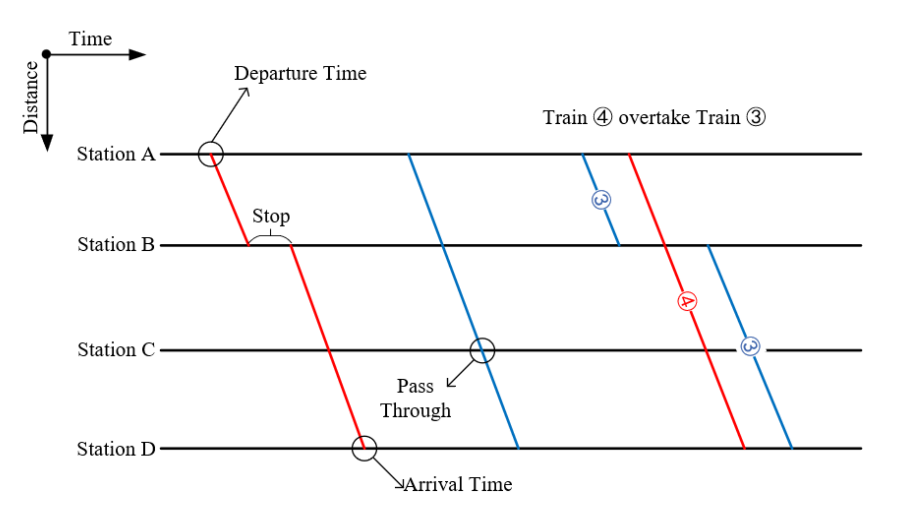
High-speed railway (HSR) has become a main trend in rail development worldwide. It not only has obvious energy-saving and environmental protection effects, but more importantly, it has a unique “electricity instead of oil” function. Therefore, it greatly reduces the dependence of the entire transportation on oil, optimizes the energy consumption structure, reduces carbon emissions, and contributes to the sustainable development of energy and the realization of a “low-carbon economy”. In recent years, HSR has developed rapidly across the world, especially in China. The scale of the HSR network has greatly expanded. The operation complexity has increased geometrically, making it necessary to respond to the travel demands of passengers in a timely and high-quality manner. Not responding to travel demands in a timely manner can result in a waste of resources, and place higher requirements on the quality (and solving efficiency) of a train’s timetable scheduling. The train timetable scheduling plays an important role in the operation of a railway line. The train timetable defines the arrival time and departure time of every train, at each station along the journey, and specifies at which station the train should stop, as well as the stop duration. Figure 1 is a schematic of a train timetable. We can see the departure and arrival times of each train, as well as whether the trains pass through or stop at each station along the journey. At the same time, we can also see that Train 3 is overtaken by Train 4.
Before scheduling a train timetable, the first thing we need to know are the passenger travel demands along the railway line. Moreover, we need to know the operation requirements of HSR, such as the interval and headway, etc.
A timetable accurately tailored to the demands of the passengers can provide high quality service to passengers and avoid the waste of resources. According to the passenger travel demands and station operation requirements, scheduling an efficient train timetable under different operation safety constraints is a complex task. Researchers face several problems while scheduling train timetables for long distance HSR lines:
Firstly, the HSR lines have complex travel demands of passengers. We say the travel demand is complex because a huge number of passengers along the railway line want to take the train every day. The Origin and Destination (O–D) of each passenger is different; moreover, the travel volume fluctuates greatly in a day. It is complex in both space and time.
Secondly, the complexity of scheduling obviously increases with the increase of the railway mileage. The longer the railway line, the more stations there will be. That means there are more safety constraints to consider and the train-to-train relationship becomes more complex.
Thirdly, the train timetable needs to be solved faster. We need to schedule new train timetables quickly in order to respond to transportation demands and different operational scenarios, such as holidays and extreme weather. It requires us to improve the solving efficiency and improve the passenger transportation service quality.
The problem of scheduling a timetable is referred to as the train timetabling problem (TTP). There are, primarily, two modeling methods for the train timetable scheduling problem: the periodic model and the aperiodic model.
To schedule a periodic train timetable, the first step is to schedule it in a short duration, mostly in one hour. Then, expand it to a full-day timetable. The third step is to modify the number of trains operating in every period, according to the fluctuation of passenger travel demands. Because the periodic timetable has strong regularity, it is convenient for passengers to remember and is convenient for passengers to transfer from one railway line to another. From an operator’s perspective, it is easier to schedule a periodic timetable because the operation complexity is simple. Usually, the periodic timetable is studied based on small- and medium-sized railway networks, and it is applied to small-scale railway networks in the real world.
For the periodic model, it is well applied in Europe and Japan, but the original periodic train timetable may not suit China, where the high-speed railway lines have much longer distances. The main reasons are as follows:
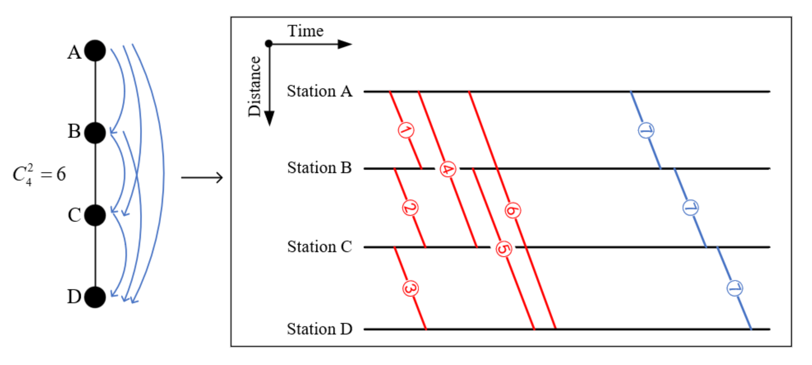
In order to meet the passenger travel demands, we may want to schedule a train for each O–D. If there are stations along the railway line, the number of O–D pairs is ; it increases greatly when the number of stations increase. Apparently, we cannot schedule a train for each O–D in the real world. Mostly, we schedule a train that stops along the journey in order to serve more than one O–D pair. As shown in Figure 2, if there are four stations, there will be O–D pairs; we can schedule six trains; moreover, we can schedule one train that serve all of the O–D pairs.
As mentioned earlier, to schedule a periodic timetable, we need to schedule a timetable for a short period. Then we copy the timetable to fill the whole day. The situation for the long-distance railway line will be more complex. There are many stations along the railway line, so the number of O–D pairs is great. If you schedule a periodic train time for long-distance railway, the total number of trains that can operate in the period is limited, as you have to schedule trains that stop many times along the journey. The travel speed of the trains will become much lower; moreover, the timetable for a short period will be repeated several times throughout the day. It means that there will be many slow trains, which will affect the service efficiency and service quality of the whole timetable significantly.
For the aperiodic model, scheduling the train timetable for a longer distance HSR also presents some difficulties. The aperiodic model has a large number of variables, so it is more difficult to solve and the solving time will be much longer. Moreover, as the distance increases, the solving difficulty increases significantly.
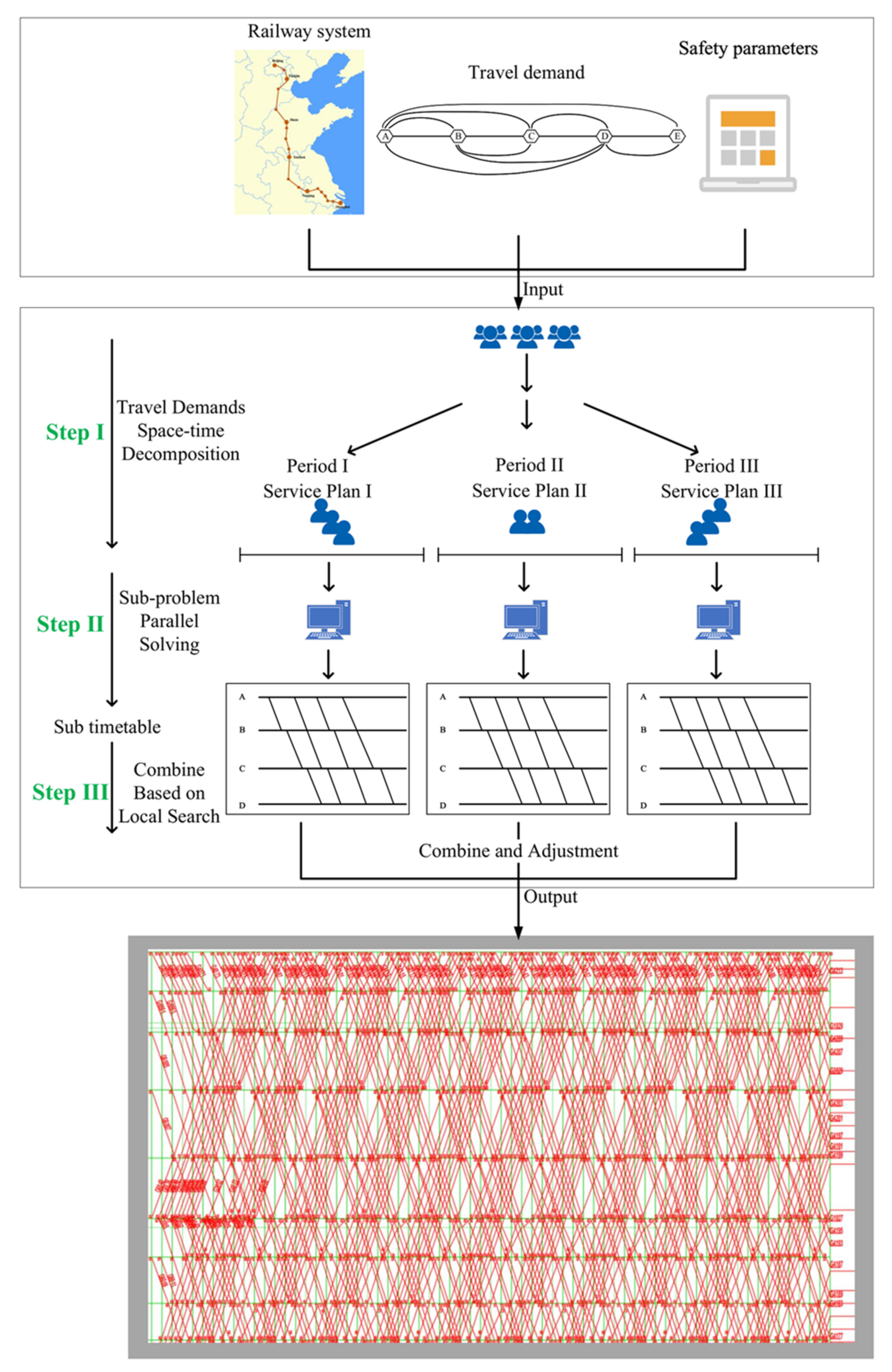
In this paper, we propose a new hybrid approach that combines the advantages of the periodic model and the aperiodic model. We aim to divide the whole day into several time periods, to reduce the difficulty of problem solving, and improve the solving efficiency, just like the periodic model. When scheduling the timetable in each period, we use the aperiodic model to meet the passengers’ travel demands more accurately and to avoid operating trains that stop too many times, improving the operational efficiency of the long-distance high-speed railway line. The framework is shown in Figure 3.
As we can see in the Figure 3, before scheduling, we need the structure of the railway line, the operation safety parameters, and the travel demands along the railway line.
The first step is to decompose the travel demands into the service plan in space and time dimensions. We introduce a technical operation plan, named the service plan. If a train departs, arrives, or passes through a station, we call the train serves the station once. The service plan defines the minimum quantity of trains at each station every day. Although the service plan only specifies the quantity of train service required at each station along the railway line, it reflects the travel demands of passengers. For the passengers of any O–D, because we specify the quantity of train service of the original station and destination station, passengers can take any of the trains to complete their journeys, considering the high frequency and efficiency of the HSR service.
In terms of space, we require the minimum quantity of train service at each station to meet the different travel demands at each station. In terms of time, we divide the whole day into several periods, and generate a service plan for each period, according to the fluctuation of passenger travel demands. During peak times, we assign a larger number of train service to transfer more passengers. Thus, we decompose the original problem into several sub-problems, both in space and time dimensions.
The second step is to parallelly solve the sub-problems in different periods by CPLEX. We designed an integer programming model for each sub-problem. In order to schedule the sub-timetables, we used parallel solving techniques to improve the solving efficiency.
The third step is to combine the sub-timetables based on a local search algorithm. Because each sub-timetable is scheduled independently, there will be some conflicts at the junction area on the timetable (due to a series of operational constraints). We used a local search algorithm to adjust the conflicts to make the timetable meet the safe operation constraints. In order to ensure the algorithm efficiency, we limit the search scope.
This paper mainly makes the following contributions to the study of the TTP:
- A space–time decomposition method is proposed to convert the complex passenger travel demands into service plans and decompose the original problem into several sub-problems;
- We designed an integer programming model for the sub-problems, and then solve the sub-problems in parallel with CPLEX in a very short time;
- We propose a local search algorithm to combine the sub-timetables under the premise of satisfying the safety constraints.
The paper is arranged as follows: in the second section, we summarize the existing research. In the third section, we describe the travel demands space–time decomposition method and discuss the influence of the number of periods. In the fourth section, we establish the integer programming method for the sub-problem. In the fifth section, we propose a combination method based on a local search algorithm. In the sixth section, we carry out a real-world case study on the Beijing–Shanghai HSR. We compare the obtained timetable with the real-world HSR timetable by different indicators. Finally, in the seventh section, conclusions and recommendations for further research are presented.
2. Literature Review
The HSR has obvious environmental protection effects. There are many interesting studies on how to make the HSR more environmentally friendly. Szkopiński [1] introduced the importance of integrating the rail transport systems. It can integrate scattered areas and improve transportation efficiency. Kuznetsov et al. [2] found a way to monitor the regenerative energy. They analyzed various factors of the influence of regenerative energy systems, and provided (environmentally friendly) ideas for saving energy during train operations. Kozachenko et al. [3] took grain transportation in the Ukraine as an example and used cluster analysis to select multiple storage sites. Then they developed a simulation model to simulate the efficiency of these sites. The results show that their method can reduce resource consumption and save transportation costs. Chen et al. [4] proposed a maximum likelihood space–time trajectory estimation model based on automatic fare collection transaction data. The model aims to analyze the transfer walk time for passengers in urban rail transit. It also provides a method for analyzing the transfer time of HSR passengers. Hou et al. [5] considered the length and the interaction force between carriages of the train with power dispersion characteristics. They designed a predictive fuzzy adaptive Proportional Integral Derivative (PID) controller based on the data of China Railway High-speed Type 3 Electric Multiple Unit (CRH3 EMU). Moreover, the simulation results show that their method is effective. Gasparik et al. [6] studied the relationship between the population, the station, and the length of transport line of the adjacent area by proposing a gravity model. They determined the railway infrastructure’s service range more accurately. By this method, they can calculate the transport potential, and then adjust the number of infrastructure projects, to achieve sustainable development.
The train timetable scheduling plays an important role in the operation of a railway line. High-quality timetables can accurately meet the travel demands of passengers, avoid a waste of resources, and achieve sustainable development. There are many interesting studies on the TTP.
For the periodic model, the basic idea is to solve the timetable in a short period of time, and extend the timetable to the whole day. The earliest research in this area can be traced back to 1989, Serasini et al. [7]. They proposed the periodic event scheduling problem (PESP) by imitated the periodic activity. Moreover, they used the implicit enumeration algorithm to solve the periodic problem. A considerable amount of the subsequent studies was carried out based on the PESP model. Voorhoever et al. [8] applied the PESP model to solve the periodic train timetabling problem. Odijk et al. [9] established a periodic time window constraint model. The model correlated arrival time and departure time in pairs. To solve the problem, they proposed a new algorithm based on constraint generation. They tested the algorithm on a medium-scale railway line and worked out a periodic train timetable. Kroon et al. [10] transformed PESP into a periodic scheduling problem. They analyzed the deficiency of existing models. They found that these models assume that the running time of all trains is fixed, but it is not fixed in real-world. On this basis, an extended model allowing partial deviation was proposed. After that, Kroon et al. [11] further studied the intersection and transfer connection of a periodic train timetable based on the PESP model on the basis of previous studies. Liebchen et al. [12] proposed the concept of managing the delay caused by emergencies in the train operation time. They constructed a multi-objective function PESP model based on the periodic train timetable. The model covered the delay transfer event and estimated the delay time. With the goal of minimizing delay, Jamili et al. [13] established a PESP model for the periodic train timetabling problem. The model set a scenario where multiple kinds of trains operated on a single-track railway. They proposed a hybrid multivariate heuristic algorithm that combined simulated annealing with particle swarm optimization. Sparing et al. [14], considering the railway capacity and robustness, chose the minimum cycle time as the stability index. They proposed a PESP model with variable train order, flexible overtaking position, and running time. They used the method of dimension reduction and iterative optimization to optimize the process of solving the PESP model. Finally, they tested the effectiveness of the algorithm in the central part of the Dutch railway network. Zhang et al. [15] introduced an extended space–time network structure. Using this structure, they reconstructed the PESP model. They used a double decomposition method, treating each train as a separate individual and adding a penalty function. They solved the running graph using a dynamic programming method.
There are some interesting studies on the periodic timetabling problem that did not use the PESP model. Heydar et al. [16] proposed a mixed integer linear programming model. They solved the periodic train timetable of a single-track railway with two kinds of trains. The optimization goal was to minimize the duration of a single period. Since then, they expanded the previous research, adding the types of stop modes set in the model. Moreover, they compared the optimization effects under different train orders [17]. Sels et al. [18] set up a mixed integer linear programming model and set the minimum travel time as optimization goal. They considered the robustness, while minimizing travel time as much as possible. Zhou et al. [19] studied a method of scheduling a timetable with multiple periods. The timetable scheduled by this method retains the regularity of the periodic timetable. By constructing a directed graph, they established a multi-path search model. This model can simultaneously optimize the running time of trains in each period. After verification, it is found that this model is more effective for small-scale problems. Since then, they designed a model for scheduling a multi-periodic train timetable, routing the train path in the timetable. They introduced a strategy to reduce the quantity of constraints and analyzed the stability and the performance of the method [20]. Robenek et al. [21] studied a method of scheduling a periodic timetable centered on passenger travel demand. They replaced the passenger satisfaction function with a travel demand forecast model. They simulated the competition of the operation company and used a calibrated logit model to reflect passenger travel demand. They used the simulated annealing algorithm to solve the timetable.
For the aperiodic model, scholars mainly use integer programming to build models. Higgins et al. [22] described a model to optimize the train timetable in the single-track railway corridor. The model sets the priority of trains passing based on the number of remaining trains and the current delay time. Then, they used the priority as the order of trains passing to shorten the delay time of trains and reduce energy consumption. Ghoseiri et al. [23] adopted the multi-objective optimization model, aiming to reduce fuel consumption and shorten travel time. They considered the cost and passenger satisfaction, solving the problem of scheduling the train timetable. Zhou et al. [24] constructed a multi-objective optimization model based on the double-track railway network. The optimization goal was to minimize the waiting time of trains and minimize the total travel time. They used the branch and bound algorithm to solve the timetable of trains with two speed classes. Since then [25], they studied the single-track train timetabling problem. They found that both the section capacity and the station capacity are limited resources. Based on the conclusion, they added a set of operation constraints. Then, they used the branch and bound algorithm and the Lagrangian relaxation algorithm to calculate the train timetable. The timetable limits the total train travel time and minimizes the train delay under the condition of limited resources. Sun et al. [26] considered the average train running time, energy consumption, and passenger satisfaction, and established a multi-objective optimization model. They designed an improved genetic algorithm to solve HSR train timetabling problem. Finally, they tested their method on a small-scale railway system. Yue et al. [27] proposed a new method based on the Lagrange relaxation algorithm and the column generation algorithm. They incorporated the passenger service demand into the schedule. At first, they used the Lagrangian relaxation algorithm to transform the problem into a linear system. Then they obtained the timetable based on the column generation algorithm. They found that their method could increase the line capacity based on the existing line conditions without adding new facilities and equipment after testing it on Beijing–Shanghai HSR system. Tong et al. [28] proposed a three-dimensional space–time network. Based on that network, they calculated the train timetable and routes together. They used a train timetable compilation method in the railway corridor. They designed a dynamic programming algorithm covering numerical processing (the numerical processing can linearize non-linear problems). Wang et al. [29] studied the train timetabling problem of HSR, and used column generation algorithms to solve the train timetable. In addition, they proposed an acceleration scheme. The scheme improves the problem of the slow solution speed of the column generation algorithm.
3. Travel Demands Space–Time Decomposition
We designed a space–time decomposition method. This method decomposes the passenger travel demands from two dimensions of space and time, and generates a service plan for each station at different periods. The service plan of each period will be the input parameters and we will solve sub-timetable for each period according to its service plan in the next step.
3.1. Travel Demands Space Decomposition
As stated above, we introduced a technical operation plan named the service plan. If a train departs, arrives, or pass through a station, we call the train serves the station. The service plan defines the minimum quantity of train service at each station every day. The space decomposition converts the passenger demands into the service plan.
For a station that serves only one railway line, we use the following method to calculate the minimum quantity of train service. The quantity of trains refers to the total number of trains that depart, arrive, or pass through this station:
means the number of passengers served by station in one day, and means the capacity of a train. means the average capacity utilization of the trains arriving at the station . It is important to note that the values are different in different train operational directions at the same station.
For the hub station, it serves several railway lines. The calculation method for the minimum quantity of trains is as follows:
means the number of passengers served on the railway line in one day, means the sum of passengers served on all the railway lines passing through station in a single day.
Before scheduling the train timetable, we generate a group of trains, and default that all the trains operate from the starting station to the terminal station of the railway line, to make sure the service capacity of the train group is far more than the passenger demands of the railway line. During the later scheduling process, we will delete some trains or cut some trains’ running distance short, considering the operational safety constraints.
The total number of trains in the group is :
Apparently, the service capacity of the train group will be bigger than the real-world timetable, because not all of the passengers take the whole journey of the train. Typically, a train serves more passengers than its capacity during the train’s journey.
3.2. Travel Demands Time Decomposition
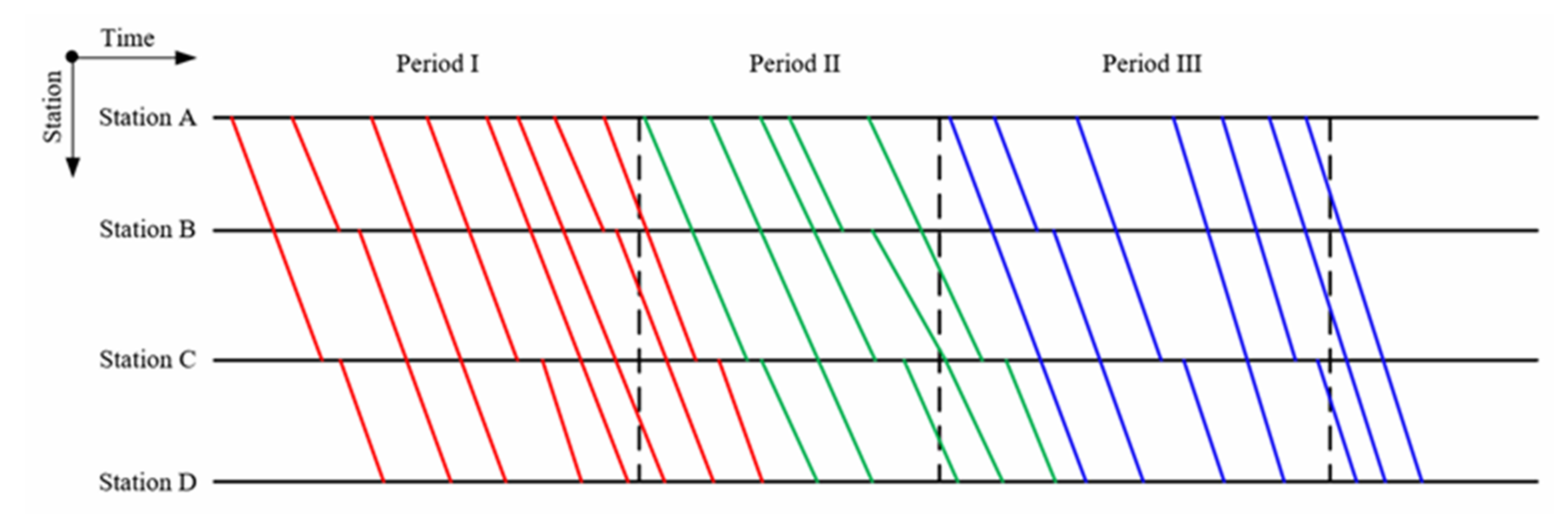
After the space decomposition, we divide the whole day into several periods and generate a service plan for each period in the time dimension, according to the fluctuation of passenger travel demands. In this way, the timetable scheduling of each period will be an independent sub-problem.
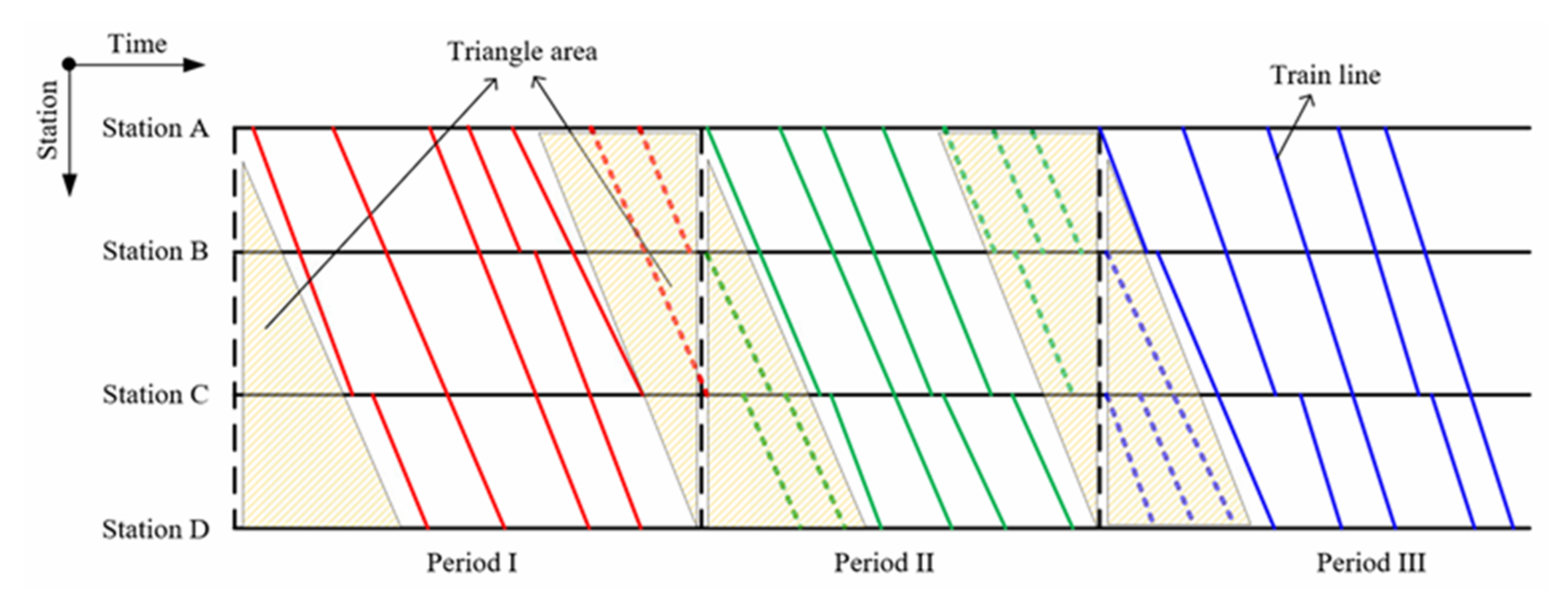
Firstly, for long-distance HSR, we do not require all trains to operate in a period strictly. If we do so, only a few trains can be operated in the period. It takes a long time for a train to run through the whole journey; thus, a lot of time would be wasted at the junction of two adjacent time periods. As shown in Figure 4, there are still some trains that could be scheduled in the yellow space; we call it the “triangle area”. If it takes 5 h for a train to run through the whole journey, for example, the triangle area will be huge.
Of course, we can schedule some trains with short running distances to fill the triangle area, such as the dotted line in Figure 4. However, the passengers may need to transfer between trains and we may need more trainsets to carry out the schedule.
We do not require all trains to operate in a period strictly, so we can schedule trains with long running distance in the triangle area, as shown in Figure 5. However, we would have to deal with unavoidable conflicts between the trains after obtaining the sub-timetables, because we solve the sub-problems independently.
When dealing with the conflicts, we have to do some adjustments on the trains, such as adjust the arrival time, departure time of the train, or cut the train’s running distance short, in order to meet safety constraints. The process of resolving a conflict between two trains is called an adjustment.
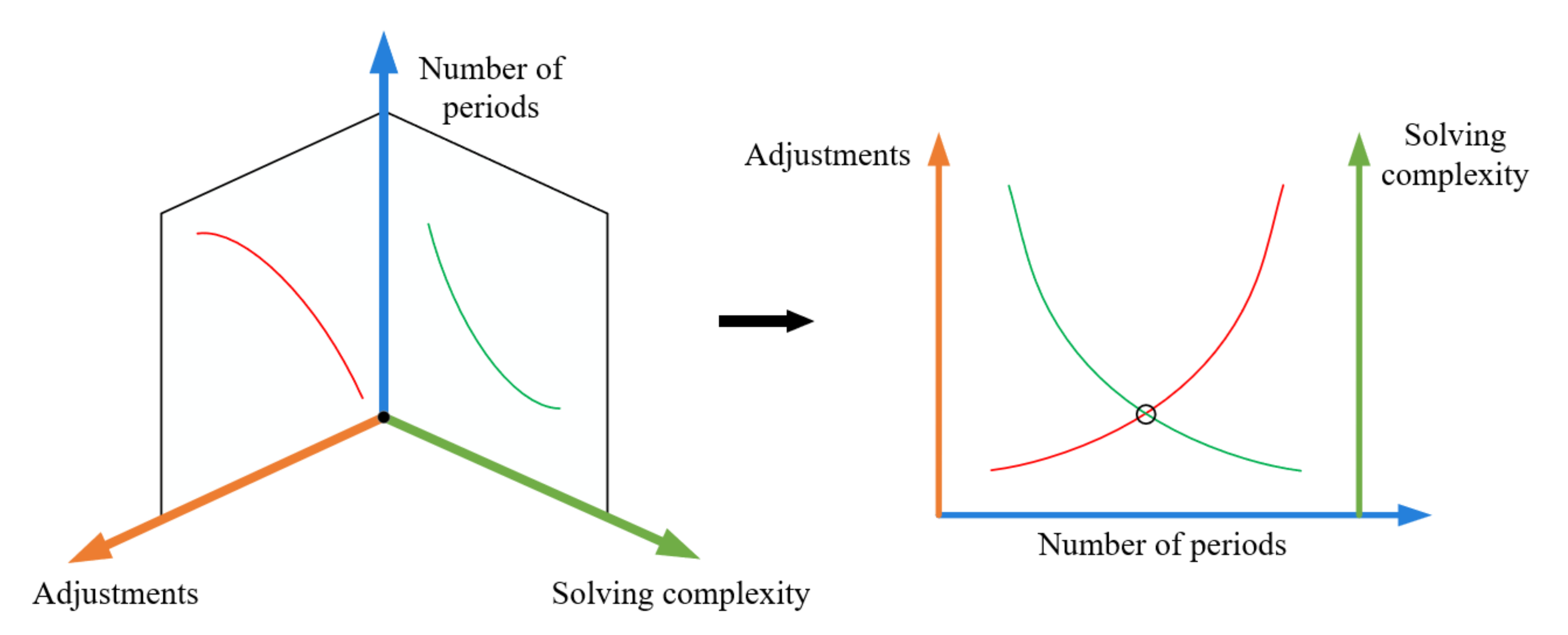
Secondly, we have to decide how many periods to divide. As can be seen from Figure 6, more periods mean more adjustments and less solving complexity. Conversely, less periods mean less adjustments and more solving complexity. We want to achieve the balance between the number of adjustments and the solving complexity by controlling the number of periods, to ensure the quality of the timetable, while spending as little solving time as possible, which is also shown on the right of Figure 6.
Thirdly, after the number of periods is determined, the service plan for each period shall be formulated according to the travel demands of passengers.
The calculation method for the quantity of trains at station in period , is as follows:
is the number of passengers in period , is the total number of passengers and is the quantity of trains at station .
If station is a hub station, the quantity of trains at station in period , should be calculated as follows:
The calculation method for the number of trains in the group in period is as follows:
is the number of passengers in period , and is the capacity of a train.
4. Sub-Problem Mathematical Model
4.1. Model Description
For now, we have obtained a group of trains for each period and the minimum quantity of train service for each station in the period. We have to schedule the departure time, arrival time, and stop strategy of each train, at each station, to optimize the sub-timetable. We present an integer programming model for the sub-problem and use CPLEX to solve sub-problems in parallel.
4.2. Model Preprocessing
Before setting the mathematical model to solve the train timetable, something needs to be done to reduce the solving complexity.
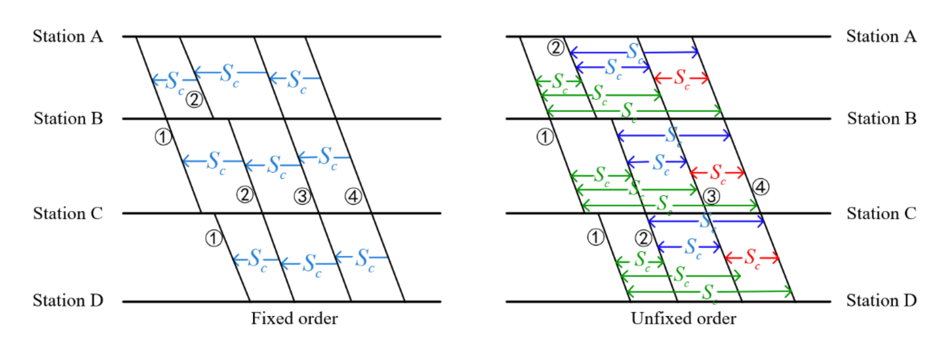
Firstly, we should determine the order of the trains. When we schedule the train timetable, one method is to arrange trains in fixed order. Another method is to not fix the order of trains; it means that the arrival time and departure time of each train must be restrained with each other. The comparison of the two constraint modes is shown in Figure 7.
As shown in Figure 8, if we schedule a train timetable with a fixed train order, we need to make sure that the adjacent trains meet the safety constraints. The safety constraints is a collection of constraints, including the constraints in section and the constraints in station, and so on. As shown in the left half of Figure 8, train 2 only needs to keep a safety interval with train 1, and train 3 only needs to keep a safety interval with train 2. The constraints are liner. If the train order is unfixed, these trains need to keep a safety interval from all the other trains. As shown in the right half of Figure 8, train 1 needs to keep a safety interval with train 2, train 3, and train 4, for example. Because we do not know which train is ahead when setting constraints, absolute values need to be introduced to keep the trains at a safe distance. Thus, the constraints are nonlinear
For example, if the order is fixed, the departure interval constraint of train and train at station is:
Moreover, if the order is not fixed, the constraint will be:
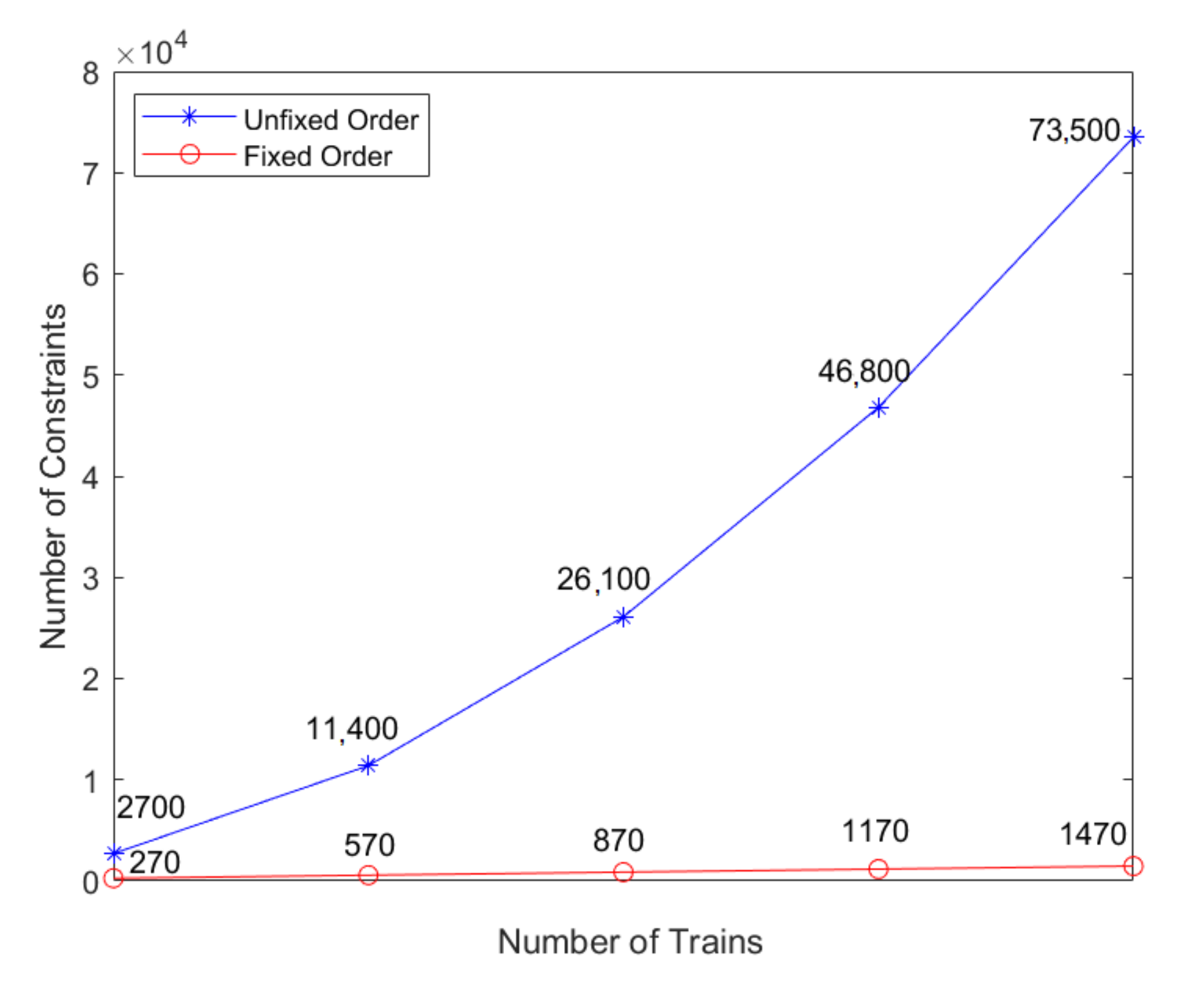
where is the number of stations and is the number of trains. The number of constraints of unfixed order and fixed order is shown in Table 1.
We can see from Figure 8 that, if , as the number of trains grows, the number of constraints of unfixed order increases faster. Thus, in this paper we schedule trains in fixed order.
4.3. Notation
4.4. Functions and Constraints
The objective function. From the passenger perspectives, they want to reach their destinations as soon as possible. From the operator perspectives, in order to improve the transport efficiency, and improve the train set utilization, they also want to reduce the train running time. Thus, we set the objective function to minimize the sum of train running time. If the train timetable scheduling problem has been divided into periods, the amount of trains in period is , we get the objective function as follow:
Departure time constraints. In a HSR system, the railroad and other facilities need periodic inspection. Maintenance workers must overhaul the whole system in non-operation hours, called the “maintenance skylight”. Thus, the HSR only operates during the operating hours, and the length is . If means the starting time of the operation hours, and we generate periods, there will be a time constrain for each train’s departure time in period :
Interval constraints. There is a time interval between trains in order to make the operation safe. They are departure interval, arrival interval, and headway. The departure interval should be constrained as follows:
The arrival interval should be constrained as follows:
Similarly, the departure time interval and the arrival time interval should also be longer than the headway:
Considering the robustness of the timetable and the solving complexity, the above constraints can be rewritten in the following form:
Dwell time constraints. If a train stops at a station along its journey, the dwell time should be longer than a minimum dwell time standard, because it takes time for the passengers to get on or get off the train. Let be the minimum dwell time of station , and let , if train stops at station , , otherwise . Thus, the dwell time should be constrained as follow:
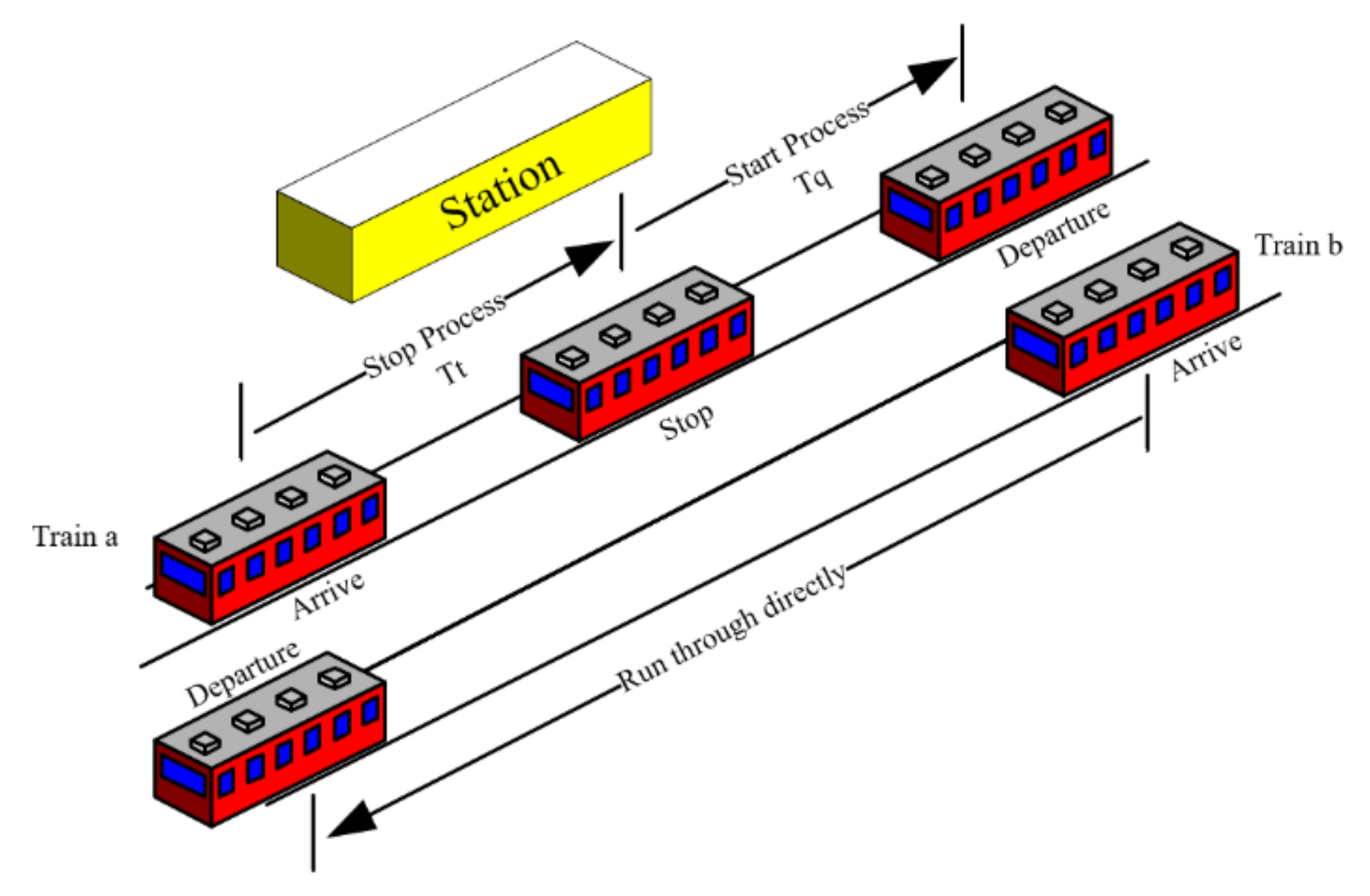
Running time constraints. A train does not run at a constant speed. It accelerates or decelerates when getting in or out of the station. As shown in Figure 9, train stops at the station and does not stop. Train needs to decelerate to stop before entering the station, and needs to accelerate to the normal operating speed when exiting. The two processes of stopping and starting are longer than train . Thus, there must be start additional time and stop additional time with the train running time in the section.
The quantity of train service constraints. According to the service plan, each station needs a certain number of trains to satisfy the travel demands of passengers. Thus, the train service constraints are as follows:
Maximum number of stop constraints. If the train stops too many times, the running time will be too long, affecting the travel efficiency of passengers. The impact is particularly strong on long-distance railway lines, where it takes a much longer time for the trains to complete the journey. In order to ensure the running time of a single train is not too long, the maximum number of stops for a train should be constrained as follows:
Station capacity constraints. The capacity of the station is limited; we need to consider the constraints of station capacity. If is the capacity of station , the station capacity constraints shall be as follows:
5. Sub-Problem Combination
After the sub-problems are solved independently and the sub-timetable is obtained, we need to combine the sub-timetables to obtain the timetable of a day.
5.1. Combinations Based on Local Search
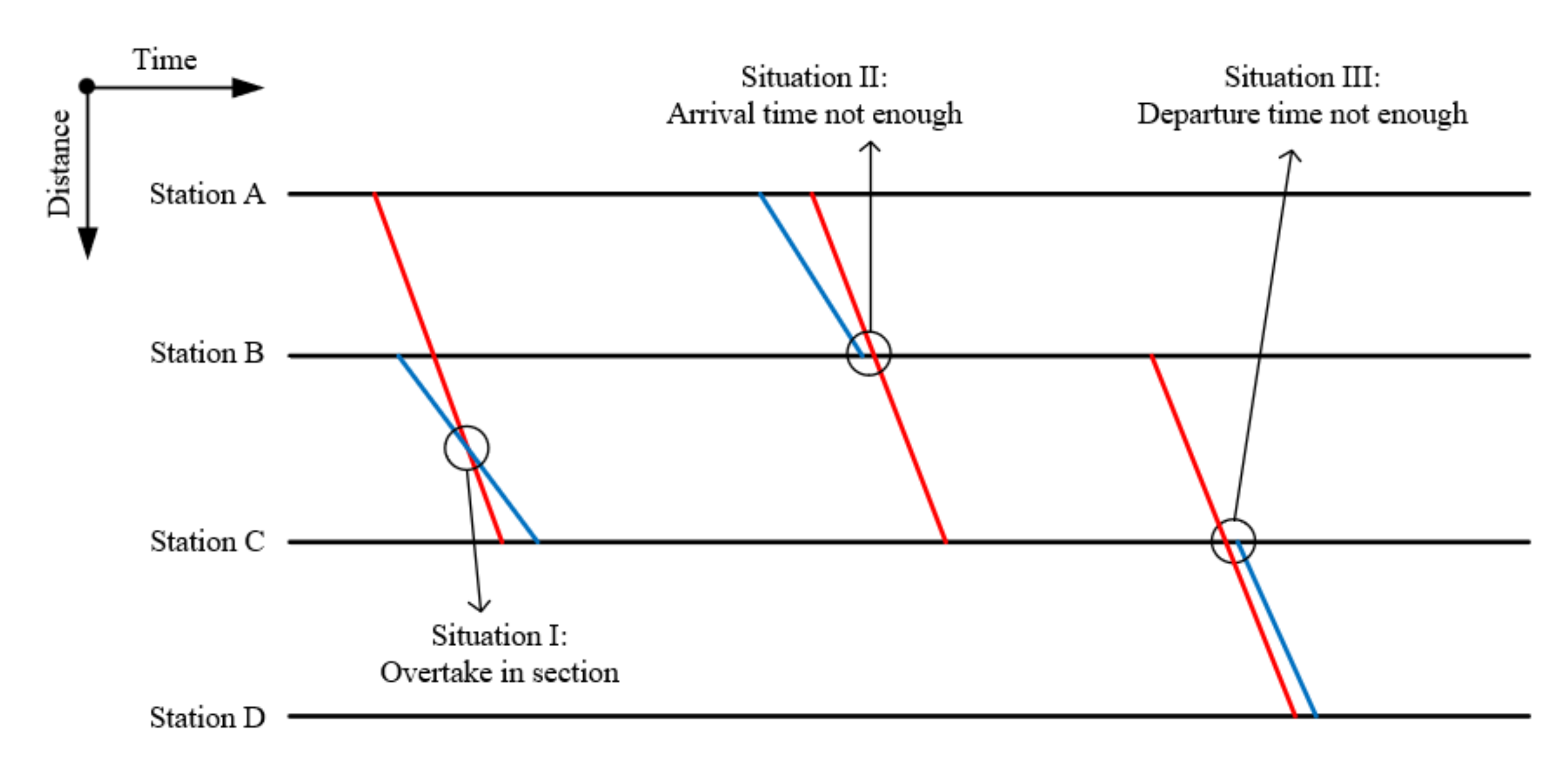
As mentioned above, because the sub-problems are solved independently, there will be conflicts between adjacent periods. Three situations do not meet the safe operation constraints, as shown in Figure 10.
The first situation is that two trains cross at a section. This is impossible in practice because there is only one track in the same operational direction between the stations, and the train behind cannot overtake another train in the section.
The second situation is that the interval of arrival times of adjacent trains does not meet the safety constraints.
The third situation is that the interval of departure times of adjacent trains does not meet the safety constraints.
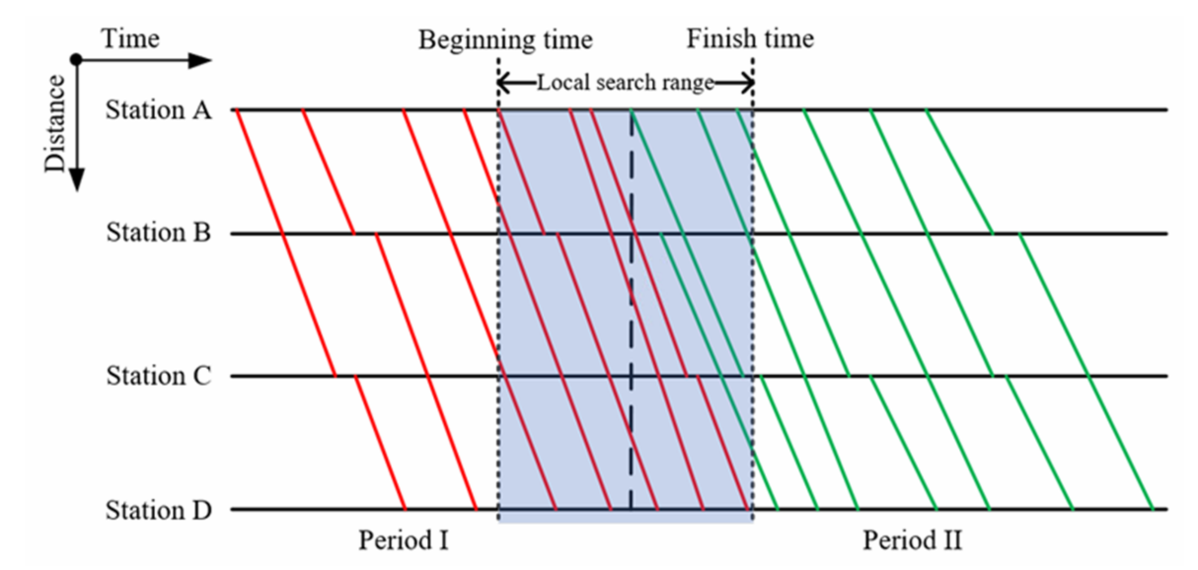
Apparently, there is no conflict between the trains in the same period, because we solve the sub-timetable with safety constraints. Conflicts only occur at the junction of adjacent sub-timetables. We propose a search and adjustment method based on local search, to adjust the conflicts between sub-timetables. The beginning time of the local search range is the departure time of the first train, whose arrival time at the terminal station exceeds the period it belongs to. The finish time of the local search range is the arrival time of the last train, whose arrival time at the terminal station exceeds the period it belongs to, as shown in Figure 11.
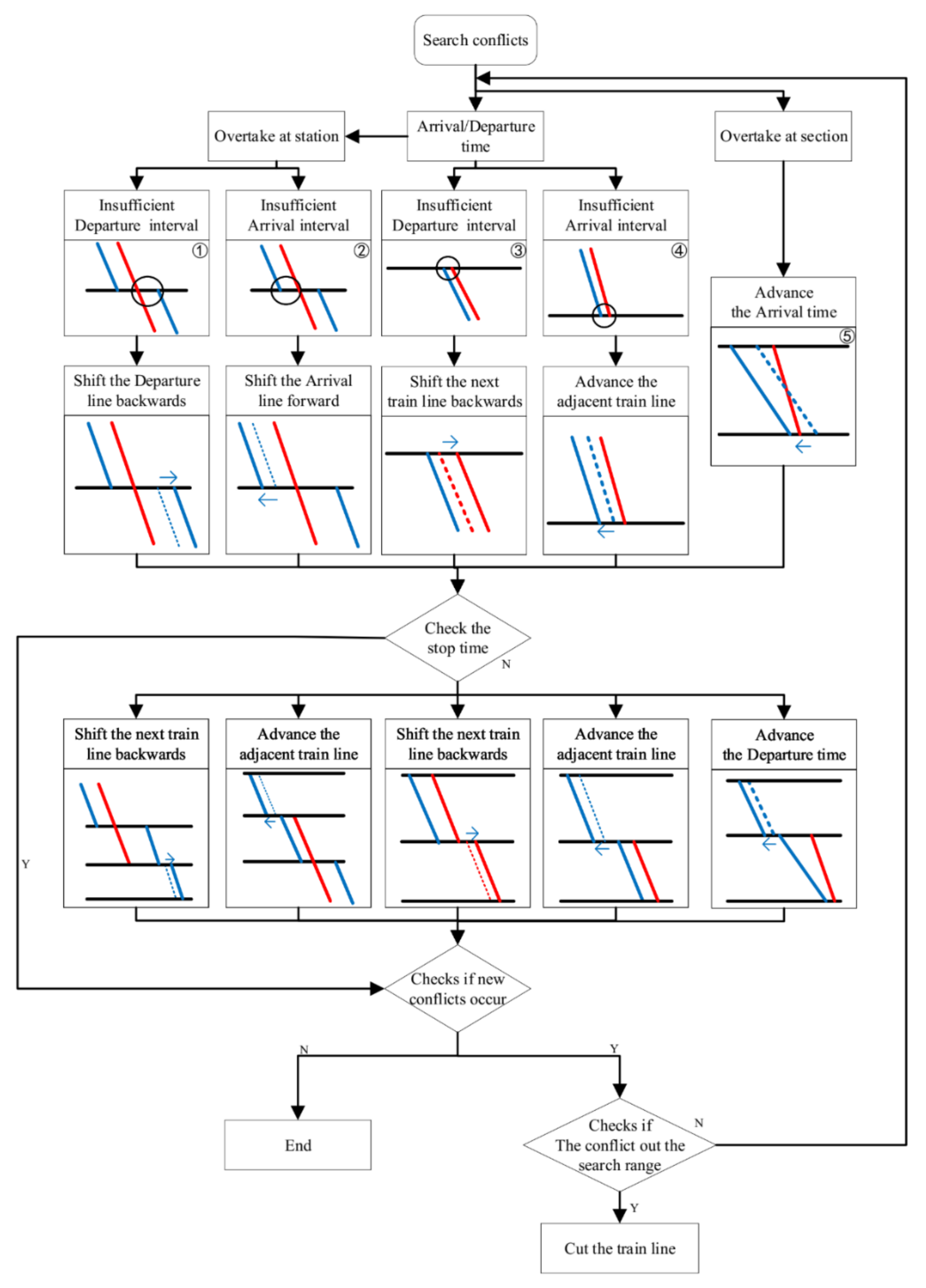
We propose a set of principles for adjusting the trains to resolve the conflicts, as shown in Figure 12.
For conflict 1 and conflict 3, under insufficient departure times, we delay the departure train line. For conflict 2 and conflict 4, under insufficient arrival times, we advance the arrival train line. For conflict 5, we advance the departure time of the train, where departure time is earlier. These adjustments may result in insufficient dwell times at stations connected by the adjusted train line, according to Equation (15). We solve this problem by moving forward or backward on the train line connected by the stop.
After all of the above adjustments are complete, it is necessary to check whether there are any new conflicts during the adjustment process. If not, the adjustment is complete. If there are new conflicts, we repeat the adjustment according to the above principles in the search range. If such adjustments still fail to meet the safety constraints, the operating line will be cut the train running distance short (or be deleted) to meet the safety operation constraints.
The train line is not cut at the nearest station. Some stations cannot be used as terminals, considering the train set depot locations. It should be cut at a station that can be used as a terminal.
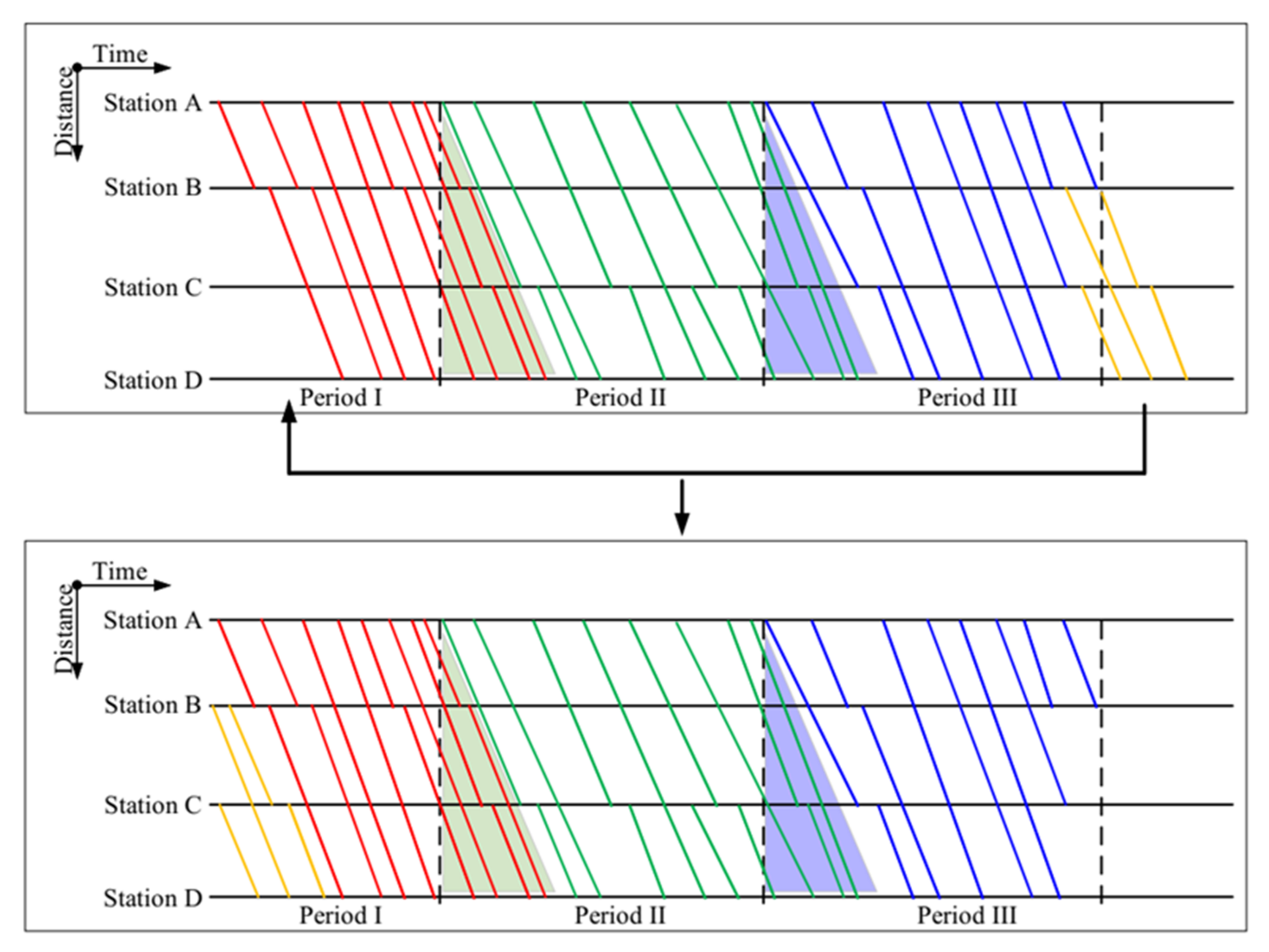
5.2. Triangle Area Train Supplement Method
The triangle area, introduced in section II, is also a part that we should make full use of, in order to operate as many trains as possible and serve more passengers. We proposed a method to fill the triangle area, as shown in Figure 13.
Because we do not limit the arrival times of trains in each period, there will be some trains running out of the period. Thus, we can fill the triangle area by this part of trains. As shown in Figure 13, period II is filled by part of the train line in period I. Moreover, the triangle area of period III is also filled by part of the train line in period II.
For the triangle area in period I, we fill it by the train line, running out of the range of period III. We cut the train line into two parts at the station, which can be a terminal, and move the train line to period I.
6. Case Study
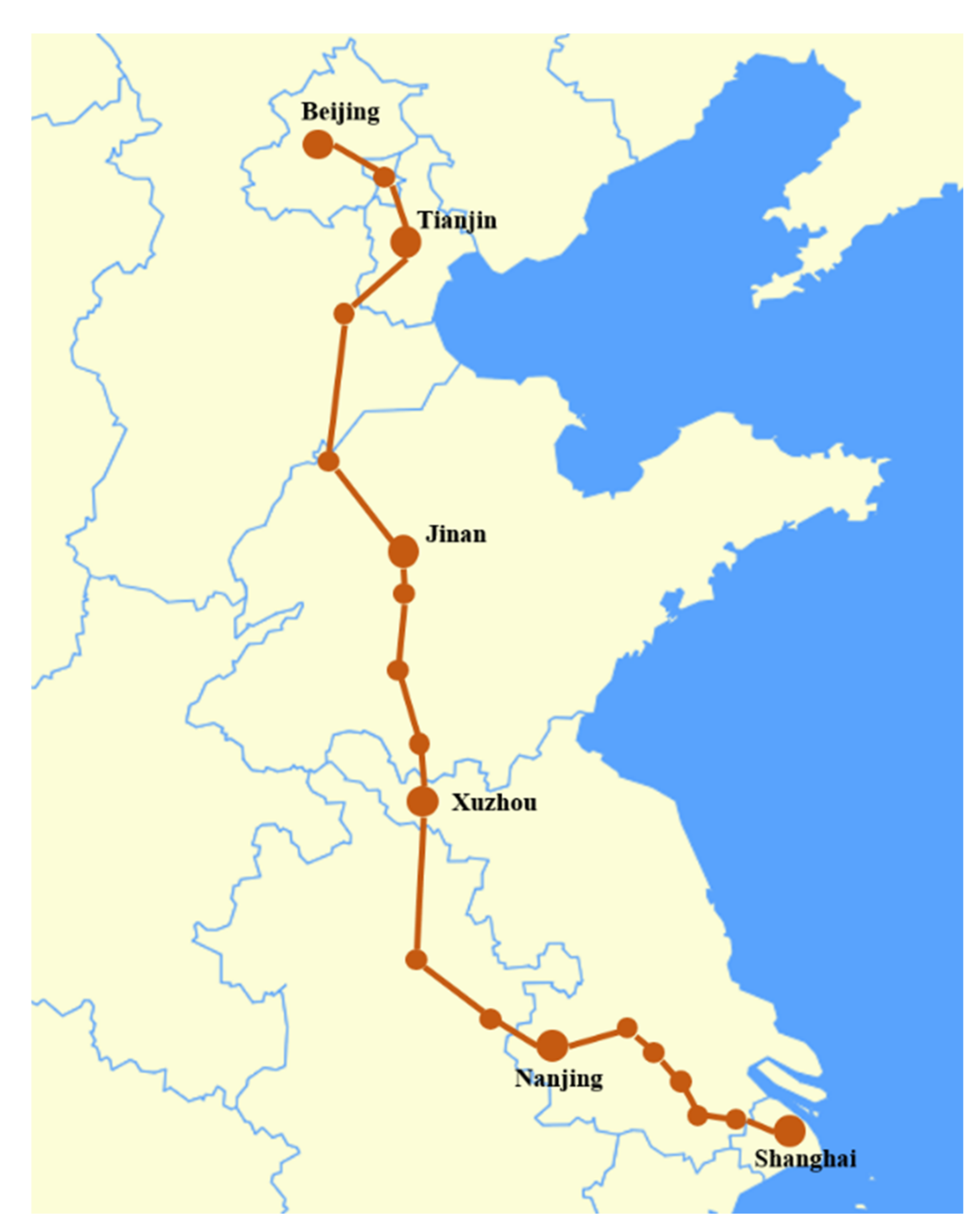
In order to verify the feasibility of the model and algorithm, the real-world data of Beijing–Shanghai HSR was used as an example to analyze. The Beijing–Shanghai HSR starts from Beijing Nan Railway Station, passes through Beijing, Tianjin, Hebei, Shandong, Anhui, Jiangsu, and Shanghai, and ends at Shanghai Hongqiao Station. It is one of the four mainly vertical HSR lines in China with a total length of 1318 km. The maximum operational speed of this line is 350 km/h, and the train can run through the whole journey within 5 h. There are 23 stations along the railway line. Figure 14 shows the Beijing–Shanghai HSR line.
6.1. Parameters and Model Processing
According to the space–time decomposition method, we calculate the quantity of the train service based on the number of passengers of the Beijing–Shanghai HSR. The quantity of trains and the dwell time standards at each station is shown in Table 4. Dwell time is the minimum time required for passengers to get on and off the train, if the train stops at a station along its journey. It should be noted that, we do not constrain the minimum dwell time for the trains at Beijing Nan station or at Shanghai Hongqiao station, because Beijing Nan is the starting station and Shanghai Hongqiao is the terminal station of the railway line. Trains only depart from Beijing Nan and terminal arrive at Shanghai Hongqiao. As explained above, the dwell time is the minimum time required for passengers to get on and off the train, if the train stops at a station along its journey, so there is no value in the corresponding cells. It should also be noted that trains at the two stations need some time for passengers to get on or get off; the required time is closely related with the train set shunting plan scheduling or the train set utilization scheduling. When scheduling the train timetable, we do not take the dwell time at the two stations into consideration. The number of trains, and other operation parameters, are shown in Table 5.
According to the operation time of Beijing–Shanghai HSR (6:00 a.m.–12:00 a.m.), we set the total operation hours from the following formula.
6.2. Results and Analysis
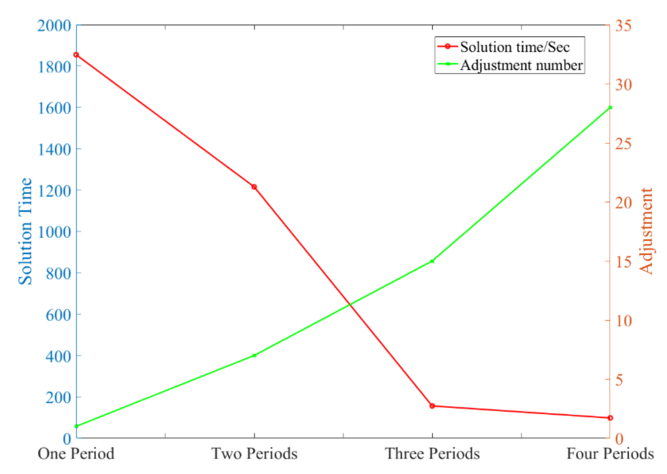
Comparing the solving efficiency of different periods. We divide the operation times into different periods and solve their respective train timetables using the algorithm in the fourth section. Then, we compare their solution times and the number of adjustments. Apparently, the less time it takes, the higher the solving efficiency the case has. The more adjustments it has, the more time it will take to obtain a feasible solution, and will reduce the quality of the original optimized solution, as mentioned before.
Figure 15 shows the comparison of the solution time and the number of adjustments. Table 6 shows the specific data of solving time and the number of adjustments for different periods.
It is obvious that, if we do not divide the operation time into periods, in case I, it is just an aperiodic model case.
According to these results, we can see that there is only one adjustment in case I, but it consumes about 30 min to get a feasible train timetable. It is not suitable for quickly scheduling the timetable, because the solution time is too long. This problem also occurs in case II, it takes about 20 min to obtain a feasible timetable, and its adjustment number is more than case I. In case III, the solution time is decreased significantly compared to case I, it only takes 2.5 min to schedule the train timetable, which is 91.7% lower. As for case IV, the solution time is shorter, but the number of adjustments is 1.87 times that of case III.
We can see that when the number of periods is more than two, the solution time is decreased significantly. From the solving efficiency point of view, they are both acceptable in case III and case IV, because their solution times are less than 3 min.
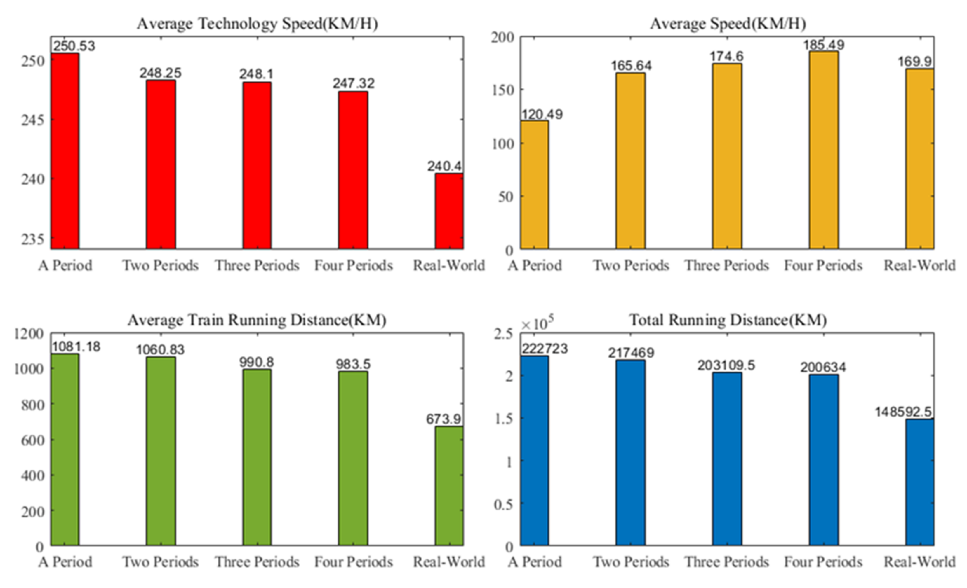
Comparing the solution quality with the real-world train timetable. The results of comparing the obtained train timetables with the real-world train timetables in different aspects are shown as Figure 16. We consider four aspects when comparing. They are average technology speed, average speed, average train running distance, and total running distance.
The average technology speed means the average speed of trains in a section. The higher the average technology speed, the higher the efficiency of the train’s utilization of the section. In terms of the average technology speed, the real-world timetable is the slowest among these timetables, 4% less than case I. The average technology speed of case I is the fastest, but compared with case II, case III, and case IV, the advantages are not obvious, only about 0.4%. Moreover, the average technology speed of case II, case III, and case IV is similar. Therefore, from the perspective of the utilization efficiency of the section, the timetable obtained by the approach in this paper is better than the real-world timetable. If the railway operation department hopes to have a higher efficiency of section utilization and a short solution time, dividing the operation time into three periods (case III) is a good choice. If there is no limit for the solution time, they do not divide the operation time (case I).
The average speed is the average speed that trains run through the whole journey, including the start addition time, the stop addition time, and the dwell time. It means the efficiency of trains run through the journey. A higher average speed means higher quality of service for passengers. Concerning average speed, we can see that the timetable in case I is about 25% lower than case II, case III, and case IV. It should also be noted that, only the two timetables in case III and in case IV are better than the real-world timetable. If the railway operation department considers passenger satisfaction as the main consideration, they can divide the operation time like case III or case IV.
In terms of the average train running distance—the longer the average train running distance means we utilize the train set more efficiently (the longer the better). Efficient utilization of the train set can save the cost of the operating department, while reducing the consumption of resources, making it more environmentally friendly. We can see that the average train running distance decreases as the number of periods increases, and each of the four cases is better than the real-world timetable.
In terms of the total running distance, a longer total running distance means more passengers could be served by trains. We can also see that the total running distance decreases as the number of periods increases, and each of the four cases is better than the real-world timetable.
Thus, from a quality solution point of view, we can see that only the two timetables in case III and in case IV are better than the real world timetables, considering all four technical aspects. Moreover, three aspects for the timetable in case III are better than the timetable in case IV, so case III is the best choice.
Overall, considering the solving efficiency and the quality solution, we can see that the case III is the best choice, because the solution quality is better, and the solving time is acceptable. Of cause, if a railway operation department only considers one main aspect, the choice may be different.
7. Conclusions
In this paper, we proposed a hybrid approach to schedule a train timetable for a long-distance high-speed railway, quickly and efficiently. The hybrid approach combines the advantages of the periodic model and the aperiodic model, provides the possibility for flexible adjustment of the timetable, according to the fluctuations of travel demands of passengers, to reduce the waste of resources and achieve sustainable development.
Firstly, inspired by the periodic train timetable scheduling model, we designed a space–time decomposition method, converting the complex passenger travel demands into service plans, and decomposing the original problem into several sub-problems. It can reduce the solving complexity of the original TTP.
Secondly, we designed an integer programming model for the sub-problems, and then solved the sub-problems in parallel with CPLEX in a very short time, compared with the aperiodic train timetable scheduling methods.
Thirdly, we designed a local search algorithm to combine the sub-timetables and deal with the conflicts between adjacent periods. We designed a rolling filling method to make full use of the triangle area, in order to operate as many trains as possible, to serve more passengers.
Fourthly, real-world data of the Beijing–Shanghai HSR was taken as an example to analyze. The results show that the timetable scheduled by the method we proposed has better performance compared with the real-world timetable, on the solving speed perspective and the evaluation indexes perspective.
It should be noted that, dividing the operation time into three periods (case III) is suitable for the Beijing–Shanghai HSR. For other railway lines, the best number of periods may be different, considering that the passenger travel demands, the operational parameters, and the total length of railway line is different. Researchers may need to test the best number of periods for their own studies, considering the solving efficiency and the solution quality.
In terms of practical applications, we did not consider the coordination of the timetable of this railway line with the timetable of other lines in the network. Thus, we will study TPP of a railway network in future research, which will be more complex and challenging, but meaningful, because the HSR has combined into a network in China and the operational influence between different railway lines is rarely studied. We would also study the train timetable rescheduling problem under some special operation scenarios, such as extreme weather or accidents. In these scenarios, the operators also need some methods or tools to reschedule the train timetable quickly and efficiently, to adapt the passenger demand fluctuations better, and minimize the negative impacts.
Author Contributions
Conceptualization, Z.W. and L.Z.; methodology, Z.W. and B.G.; software, Z.W.; data, B.G. and X.C.; writing—original draft preparation, Z.W.; writing—review and editing, Z.W., B.G., and H.Z. All authors have read and agreed to the published version of the manuscript.
Funding
This research was funded by the Fundamental Research Funds for the Central Universities, grant number 2018RC012.
Institutional Review Board Statement
Not applicable.
Informed Consent Statement
Not applicable.
Data Availability Statement
Not applicable.
Acknowledgments
The authors would like to express great appreciation to editors and reviewers for their positive and constructive comments.
Conflicts of Interest
The authors declare no conflict of interest.
References
- Szkopiński, J. The certain approach to the assessment of interoperability of railway lines. Arch. Transp. 2014, 29, 65–75. [Google Scholar] [CrossRef]
- Kuznetsov, V.G.; Sablin, O.I.; Chornaya, A.V. Improvement of the regenerating energy accounting system on the direct current railways. Arch. Transp. 2015, 36, 35–42. [Google Scholar] [CrossRef] [Green Version]
- Kozachenko, D.; Vernigora, R.; Kuznetsov, V.; Lohvinova, N.; Rustamov, R.; Papahov, A. Resource-saving technologies of railway transportation of grain freights for export. Arch. Transp. 2018, 45, 53–64. [Google Scholar] [CrossRef] [Green Version]
- Chen, X.; Zhou, L. Data-driven method to estimate the maximum likelihood space–time trajectory in an urban rail transit system. Sustainability 2018, 10, 1752. [Google Scholar] [CrossRef] [Green Version]
- Hou, T.; Guo, Y.-Y.; Niu, H.-X. Research on speed control of high-speed train based on multi-point model. Arch. Transp. 2019, 50, 35–46. [Google Scholar] [CrossRef]
- Gasparik, J.; Dedik, M. Estimation of Transport Potential in Regional Rail Passenger Transport by Using the Innovative Mathematical-Statistical Gravity Approach. Sustainability 2020, 12, 3821. [Google Scholar] [CrossRef]
- Serafini, P.; Ukovich, W. A mathematical model for periodic scheduling problems. SIAM J. Discret. Math. 1989, 2, 550–581. [Google Scholar] [CrossRef]
- Voorhoeve, M. Rail Scheduling with Discrete Sets; Unpublished Report; Eindhoven University of Technology: Eindhoven, The Netherlands, 1993. [Google Scholar]
- Odijk, M.A. A constraint generation algorithm for the construction of periodic railway timetables. Transp. Res. Part B Methodol. 1996, 30, 455–464. [Google Scholar] [CrossRef]
- Kroon, L.G.; Peeters, L.W.P. A Variable Trip Time Model for Cyclic Railway Timetabling. Transp. Sci. 2003, 37, 198–212. [Google Scholar] [CrossRef]
- Kroon, L.; Peeters, L.; Wagenaar, J.; Zuidwijk, R. Flexible Connections in PESP Models for Cyclic Passenger Railway Timetabling. Transp. Sci. 2014, 48, 136–154. [Google Scholar] [CrossRef] [Green Version]
- Liebchen, C.; Schachtebeck, M.; Schöbel, A.; Stiller, S.; Prigge, A. Computing delay resistant railway timetables. Comput. Oper. Res. 2010, 37, 857–868. [Google Scholar] [CrossRef]
- Jamili, A.; Shafia, M.; Sadjadi, S.; Tavakkoli-Moghaddam, R. Solving a periodic single-track train timetabling problem by an efficient hybrid algorithm. Eng. Appl. Artif. Intell. 2012, 25, 793–800. [Google Scholar] [CrossRef]
- Sparing, D.; Goverde, R.M. A cycle time optimization model for generating stable periodic railway timetables. Transp. Res. Part B Methodol. 2017, 98, 198–223. [Google Scholar] [CrossRef]
- Zhang, Y.; Peng, Q.; Yao, Y.; Zhang, X.; Zhou, X. Solving cyclic train timetabling problem through model reformulation: Extended time-space network construct and Alternating Direction Method of Multipliers methods. Transp. Res. Part B Methodol. 2019, 128, 344–379. [Google Scholar] [CrossRef]
- Heydar, M.; Petering, M.E.; Bergmann, D.R. Mixed integer programming for minimizing the period of a cyclic railway timetable for a single track with two train types. Comput. Ind. Eng. 2013, 66, 171–185. [Google Scholar] [CrossRef]
- Petering, M.E.H.; Heydar, M.; Bergmann, D.R. Mixed-Integer Programming for Railway Capacity Analysis and Cyclic, Combined Train Timetabling and Platforming. Transp. Sci. 2016, 50, 892–909. [Google Scholar] [CrossRef]
- Sels, P.; Dewilde, T.; Cattrysse, D.; Vansteenwegen, P. Reducing the passenger travel time in practice by the automated construction of a robust railway timetable. Transp. Res. Part B Methodol. 2016, 84, 124–156. [Google Scholar] [CrossRef]
- Zhou, W.; Tian, J.; Xue, L.; Jiang, M.; Deng, L.; Qin, J. Multi-periodic train timetabling using a period-type-based Lagrangian relaxation decomposition. Transp. Res. Part B Methodol. 2017, 105, 144–173. [Google Scholar] [CrossRef]
- Zhou, W.; You, X. A Mixed Integer Linear Programming Method for Simultaneous Multi-Periodic Train Timetabling and Routing on a High-Speed Rail Network. Sustainability 2020, 12, 1131. [Google Scholar] [CrossRef] [Green Version]
- Robenek, T.; Azadeh, S.S.; Maknoon, Y.; De Lapparent, M.; Bierlaire, M. Train timetable design under elastic passenger demand. Transp. Res. Part B Methodol. 2018, 111, 19–38. [Google Scholar] [CrossRef] [Green Version]
- Higgins, A.; Kozan, E.; Ferreira, L. Optimal scheduling of trains on a single line track. Transp. Res. Part B Methodol. 1996, 30, 147–161. [Google Scholar] [CrossRef] [Green Version]
- Ghoseiri, K.; Szidarovszky, F.; Asgharpour, M.J. A multi-objective train scheduling model and solution. Transp. Res. Part B Methodol. 2004, 38, 927–952. [Google Scholar] [CrossRef]
- Zhou, X.; Zhong, M. Bicriteria train scheduling for high-speed passenger railroad planning applications. Eur. J. Oper. Res. 2005, 167, 752–771. [Google Scholar] [CrossRef]
- Zhou, X.; Zhong, M. Single-track train timetabling with guaranteed optimality: Branch-and-bound algorithms with enhanced lower bounds. Transp. Res. Part B Methodol. 2007, 41, 320–341. [Google Scholar] [CrossRef]
- Sun, Y.; Cao, C.; Wu, C. Multi-objective optimization of train routing problem combined with train scheduling on a high-speed railway network. Transp. Res. Part C Emerg. Technol. 2014, 44, 1–20. [Google Scholar] [CrossRef]
- Yue, Y.; Wang, S.; Zhou, L.; Tong, L.; Saat, M.R. Optimizing train stopping patterns and schedules for high-speed passenger rail corridors. Transp. Res. Part C Emerg. Technol. 2016, 63, 126–146. [Google Scholar] [CrossRef]
- Zhou, L.; Tong, L.C. Joint optimization of high-speed train timetables and speed profiles: A unified modeling approach using space-time-speed grid networks. Transp. Res. Part B Methodol. 2017, 97, 157–181. [Google Scholar] [CrossRef] [Green Version]
- Wang, J.; Zhou, L. Column Generation Accelerated Algorithm and Optimisation for a High-Speed Railway Train Timetabling Problem. Symmetry 2019, 11, 983. [Google Scholar] [CrossRef] [Green Version]
Figure 1.
The schematic of a train timetable.

Figure 2.
Comparison of stop modes.

Figure 3.
Framework of the approach.

Figure 4.
Condition of junction capacity waste and triangle area.

Figure 5.
The long journey trains operated in the triangle area.

Figure 6.
Solving complexity, periods, and adjustments.

Figure 7.
The comparison of the two constraint modes.

Figure 8.
The comparison of the two constraint modes.

Figure 9.
Start additional time and stop additional time.

Figure 10.
The situation of conflicts at junction.

Figure 11.
The local search ranges.

Figure 12.
Framework of local search combination method.

Figure 13.
Filling method.

Figure 14.
Diagram of the Beijing–Shanghai high-speed railway (HSR) line.

Figure 15.
Solution time and adjustment number comparison.

Figure 16.
Comparison of timetables.


Table 1.
Solving scale comparison.
| Mode | Number of Constraints | Number of Decision Variables | Model Feature |
|---|---|---|---|
| Unfixed order | Nonlinear | ||
| Fixed order | Linear |
Table 2.
General subscripts.
| Subscripts | Description |
|---|---|
| i | Period where I is the set of sub-timetable, . |
| j | Train where is the set of trains in period , . |
| k | Station where is the set of stations, . |
Table 3.
Description of the parameters.
| Parameters | Description |
|---|---|
| The departure time of train of period in station . | |
| The arrival time of train of period in station . | |
| Whether train stop at station in period | |
| The minimum number of train service at station in period . | |
| The maximum number of stops of a train . | |
| The capacity of station . | |
| The starting time of the operation hours. | |
| The service time range. | |
| The minimum departure interval. | |
| The minimum arrival interval. | |
| The minimum headway. | |
| The start additional time. | |
| The stop additional time. | |
| The minimum dwell time of station . | |
| The shortest running time from station to . |
Table 4.
Service plan and dwell time.
| Station | Dwell Time (Minutes) | Train Service Quantity |
|---|---|---|
| Beijing Nan | - | 157 |
| Langfang | 2 | 22 |
| Tianjin Nan | 2 | 51 |
| Cangzhou Xi | 2 | 32 |
| Dezhou Dong | 2 | 35 |
| Jinan Xi | 4 | 128 |
| Taian | 2 | 32 |
| Qufu Dong | 2 | 26 |
| Tengzhou Dong | 2 | 31 |
| Zaozhuang | 2 | 26 |
| Xuzhou Dong | 2 | 101 |
| Suzhou Dong | 2 | 29 |
| Bengbu Nan | 3 | 34 |
| Dingyuan | 2 | 21 |
| Chuzhou | 2 | 38 |
| Nanjing Nan | 4 | 159 |
| Zhenjiang Nan | 2 | 24 |
| Danyang Bei | 2 | 24 |
| Changzhou Bei | 3 | 27 |
| Wuxi Dong | 2 | 26 |
| Suzhou Bei | 2 | 32 |
| Kunshan Nan | 2 | 17 |
| Shanghai Hongqiao | - | 135 |
Table 5.
Operation parameters.
| Parameters | Value |
|---|---|
| The number of trains | 205/pairs |
| Start additional time | 2/min |
| Stop additional time | 3/min |
| Headway | 3/min |
| Departure interval | 4/min |
| Arrival interval | 4/min |
Table 6.
Specific data of solving time and adjustments.
| Case | Period Number | Solution Time (Seconds) | Adjustments Number |
|---|---|---|---|
| Case I (Aperiodic model) | 1 | 1896 | 1 |
| Case II | 2 | 1262 | 7 |
| Case III | 3 | 155 | 15 |
| Case IV | 4 | 93 | 28 |
Publisher’s Note: MDPI stays neutral with regard to jurisdictional claims in published maps and institutional affiliations. |
© 2021 by the authors. Licensee MDPI, Basel, Switzerland. This article is an open access article distributed under the terms and conditions of the Creative Commons Attribution (CC BY) license (http://creativecommons.org/licenses/by/4.0/).
Share and Cite
MDPI and ACS Style
Wang, Z.; Zhou, L.; Guo, B.; Chen, X.; Zhou, H. An Efficient Hybrid Approach for Scheduling the Train Timetable for the Longer Distance High-Speed Railway. Sustainability 2021, 13, 2538. https://0-doi-org.brum.beds.ac.uk/10.3390/su13052538
AMA Style
Wang Z, Zhou L, Guo B, Chen X, Zhou H. An Efficient Hybrid Approach for Scheduling the Train Timetable for the Longer Distance High-Speed Railway. Sustainability. 2021; 13(5):2538. https://0-doi-org.brum.beds.ac.uk/10.3390/su13052538
Chicago/Turabian StyleWang, Zeyu, Leishan Zhou, Bin Guo, Xing Chen, and Hanxiao Zhou. 2021. "An Efficient Hybrid Approach for Scheduling the Train Timetable for the Longer Distance High-Speed Railway" Sustainability 13, no. 5: 2538. https://0-doi-org.brum.beds.ac.uk/10.3390/su13052538
Note that from the first issue of 2016, this journal uses article numbers instead of page numbers. See further details here.