
Multimodal Data Based Regression to Monitor Air Pollutant Emission in Factories


School of Economics and Management, China University of Petroleum (East China), Qingdao 266580, China
*
Author to whom correspondence should be addressed.
Sustainability 2021, 13(5), 2663; https://0-doi-org.brum.beds.ac.uk/10.3390/su13052663
Submission received: 25 December 2020
/
Revised: 4 February 2021
/
Accepted: 5 February 2021
/
Published: 2 March 2021
Abstract
:Air pollution originating from anthropogenic emission, which is an important factor for environmental policy to regulate the sustainable development of enterprises and the environment. However, the missing or mislabeled discharge data make it impossible to apply this strategy in practice. In order to solve this challenge, we firstly discover that the energy consumption in a factory and the air pollutants are linearly related. Given this observation, we propose a support vector regression based Single-location recovery model to recover the air pollutant emission by using the energy consumption data in a factory. To further improve the precision of air pollutant emission estimation, we proposed a Gaussian process regression based multiple-location recovery model to estimate and recover the missing or mislabeled air pollutant emission from surrounding available air quality readings, collected by the government’s air quality monitoring station. Moreover, we optimally combine the two approaches to achieve the accurate air air pollutant emission estimation. To our best of knowledge, this is the first paper for monitoring the air pollutant emission taking both a factory’s energy consumption and government’s air quality readings into account. The research model in this article uses actual data(10,406,880 entries of data including weather, PM 2.5, date, etc.) from parts of Shandong Province, China. The dataset contains 33 factories (5 types) and we use the co-located air quality monitoring station as ground truth. The results show that, our proposed single-location recovery, multi-location recovery, and combined method could acquire the mean absolute error of 8.45, 9.69, and 7.25, respectively. The method has consistent accurate prediction behavior among 5 different factory types, shows a promising potential to be applied in broader locations and application areas, and outperforms the existing spatial interpolation based methods by 43.8%.
1. Introduction
Global pollution has become a severe issue for the human being over decades. The aggravation of the global pollution is mainly caused by the excessive pollutant emission. Especially in the developing countries, which prioritizes economic growth over the environment, many low-tech factories are built close to cities, inevitably contaminating the air. The World Health Organization (WHO) [1,2] reveals that more than four million people die because of the cancer caused by PM2.5 and pollution gas penetrating into lung, heart and blood per year, especially those living in the highly polluted industrial cities.
Different countries have issued many policies to control the emission of exhaust gas, and have also adopted institutions to monitor the emission of the corresponding pollutant. Government installs the continuous emissions monitoring system at the outlets of the exhaust gas to collect real-time and fine-grained data for monitoring the status of pollution emitted by the factories. As Figure 1 depicts, the monitor system consisting of 33 sensors and information system is installed in the 33 factories.
In this paper, we focus on estimating PM 2.5 (a major and harmul air pollutant) emitted from a factory. This is not trival because the PM 2.5 sensors installed in the factory are easily modified by the factory owners. To overcome this practical issue, we smartly estimate the PM 2.5 emission from the indirect information including the energy consumption in a factory and PM 2.5 readings collected by the government’s PM 2.5 monitoring stations. To our best of knowledge, this is the first paper, considering both a factory’s energy consumption and government’s air quality readings, proposed to monitor a factory’s air pollutant emission given the unrealiable. Our detailed contributions are as follows:
- Our paper firstly discovers the linear relationship between the air pollutant (PM 2.5) and the energy consumption in a factory (Section 3 Preliminary Study), which is monitored by the power plant and government and cannot be modified by factory owners. Despite the difficulty to collect the true emission of pollutants, the indirect factors (energy consumption) are usually easy to obtain. The intuition is that we could recover the missing or mislabeled air quality values from those indirect features, which is referred to as Single-location recovery. Supporting vector regression (SVR) model is used to establish the relationship between the emission of pollutants and the indirect factors of energy consumption and material balance. Specifically, we use the data to train the SVM model and then apply this model to estimate the emission of pollutants of a factory given the indirect factors of this factory.
- To further improve the precision of air pollutant emission estimation, we combine the spatial interpolation based multiple-location recovery model and the single-location recovery model to obtain the precise air pollutant emission estimation. Specifically, we apply the gaussian process regression (GPR) model to generate an accurate air quality map at each timestamp and recover the missing or mislabeled air quality values at unknown locations. To combine the recovered air quality values from the above mentioned two models, a weighted scheme is applied.
- We evaluate the proposed models using real-world data in Shandong Province, China, which contains 33 factories categorized into 5 types and each has a co-located air quality monitoring station. We also compare our model with the existing spatial interpolation based models and evaluate our model under different seasons. To the best of our knowledge, this paper is the first data-driven pollution emission estimation model for Chinese factories.
The paper will first give the review of related works, then follows a Preliminary Study to show the opportunity of estimating air quality values based on indirect factors and the motivation to use spatial interpolation for air quality recovery task. To solve the above-mentioned problems and challenges, our SVR based, GPR based and combined models are described in the method section. Finally, we will give the experiment evaluation results on the real-world dataset and give the suggestions.
2. Literature Review
In order to control the pollutant discharge of factories, governments of various countries have formulated different pollutant discharge ranges and rigid systems for severe penalties for excessive discharge according to their national conditions. However, researchers believe that compared with simple punishments, the key to resolving contradictions is to formulate flexible policies that can guide the coordinated development of the environment and the economy [3,4,5]. Empirical research shows that environmental taxes, as representatives of flexible policies that promote energy conservation, emission reduction, and green technology development, play an important role in preventing pollution [6] and improving environmental quality [7]. Onofrei [8] analyzed the data of 20 European countries from 1994 to 2012 and found that environmental taxes can effectively reduce greenhouse gas emissions. Agnolucci [9] did research on Germany and Paris and showed that environmental tax reform can substantially reduce energy consumption and carbon emissions.
Researchers have provided many references for the government to adjust environmental policies in a timely manner by analyzing the impact of pollutant discharge on the environment [10]. In order to quantify the air environmental policy, Chalabi et al. [11] established a corresponding system framework. Boyce et al. [12] believed that by reducing the emission of common pollutants such as fossil fuel combustion, co-benefits of air quality can be produced. At the same time, studies have shown that traffic control policies can reduce air pollution in the short term [13]. Gao et al. [14] proposed that compared with rigid commanded emission reduction policies, flexible-oriented policies can better improve the environment. Yang et al. [15] taking Beijing residents as an example, traced the PM 2.5 footprint and driving factors.
It is worth noting that no matter what kind of environmental policy is, it needs to be based on real pollution data to play its corresponding effect. To this end, many researchers have done a lot of research from the perspective of pollutant emission monitoring technologies and methods [16,17,18,19,20]. Satellite monitoring can not only reflect the current surface conditions from time to time, but also monitor pollution problems in the ocean. Eronat [21] pointed out that in order to detect pollution in time, the use of satellites is necessary to monitor the bay. Aliyu & Botai [22] collected urban features through satellites and effectively assessed the content of certain gas components in the urban atmosphere. Khaki & Awange [23] invented a portable air quality testing device and used Nigeria as an experimental sample, the results show that the device is stable and reliable. The air quality sensor can detect the air quality of the surrounding environment. Li et al. [24] found that mining PM sensor data can not only retain the characteristics of pollutants, but also greatly enhance the spatial distribution of pollutants. Through research, Dewinter et al. [25] introduced the change of PM 2.5 concentration within 20 m on both sides of the road.
The factories, however, might modify the monitoring system, including attaching fans at the air quality sensors, to fake the data of emissions for maximizing the benefits. According to China Statistical Yearbook 2019, the emission of exhaust gas is about 29 million tons in China. Meanwhile, according to the People’s Daily, the Chinese State media, 10% of the more than 10,000 companies investigated by the Ministry of Environmental Protection had faked emissions data in 2015. If the true emissions of pollutants are conservatively accounted as 5% of the reported data, at least 1.45 million tons of exhaust gas is illegally emitted by the factories in China, causing economic loss up to 2 billion US dollars. Unfortunately, despite the severe punishments are issued, it is very hard for the government to prevent this totally since the cost to employ personnel to monitor the factories is not affordable. Thus, it is urgent to find an effective approach to monitor the true emissions of pollutants in a factory.
Despite the lacking of research on monitoring the air pollutant emission given the unreliable air pollutant sensor data, there are many spatial interpolation based models were proposed to monitor the air quality. Cheng et al. [26,27] evaluate different kinds of spatial interpolation methods and concludes that Gaussian Process (GP) Regression are most accurate PM 2.5 interpolation method. Gao et al. [28] using atmospheric chemistry models to quantitatively analyze the effects of electricity generation in China and India on PM 2.5 concentrations. However, their approach merely rely on the local sensor readings, which may not be reliable and accurate. Our proposed method is different from state-of-art PM 2.5 spatial interpolation works: (i) We first predict the PM 2.5 values from local indirect energy consumption facots to improve the accuracy of PM 2.5 values; (ii) we then combine the single-location recovery with the multilocation recovery readings with a trade-off parameter.
In summary, the research on environmental pollution control mainly focuses on the impact of macro-policy and macro-emission control [29,30,31]. In order to ensure the effectiveness of the policy, the authenticity of emissions data is very critical. Although the monitoring equipment can directly reflect the state of pollutant discharge [32,33,34], it is impossible to distinguish the illegal discharge behavior that bypasses the monitoring point [35,36,37,38,39]. The lack or distortion of micro-level data not only leads to the failure of environmental policies, but also produces the effect of bad money driving out good money, allowing factories that illegally discharge pollutants to occupy the market share of legitimate factories [40,41,42,43,44]. If this continues, it will not only cause a lot of environmental pollution, but also disrupt the market order.
3. Preliminary Study
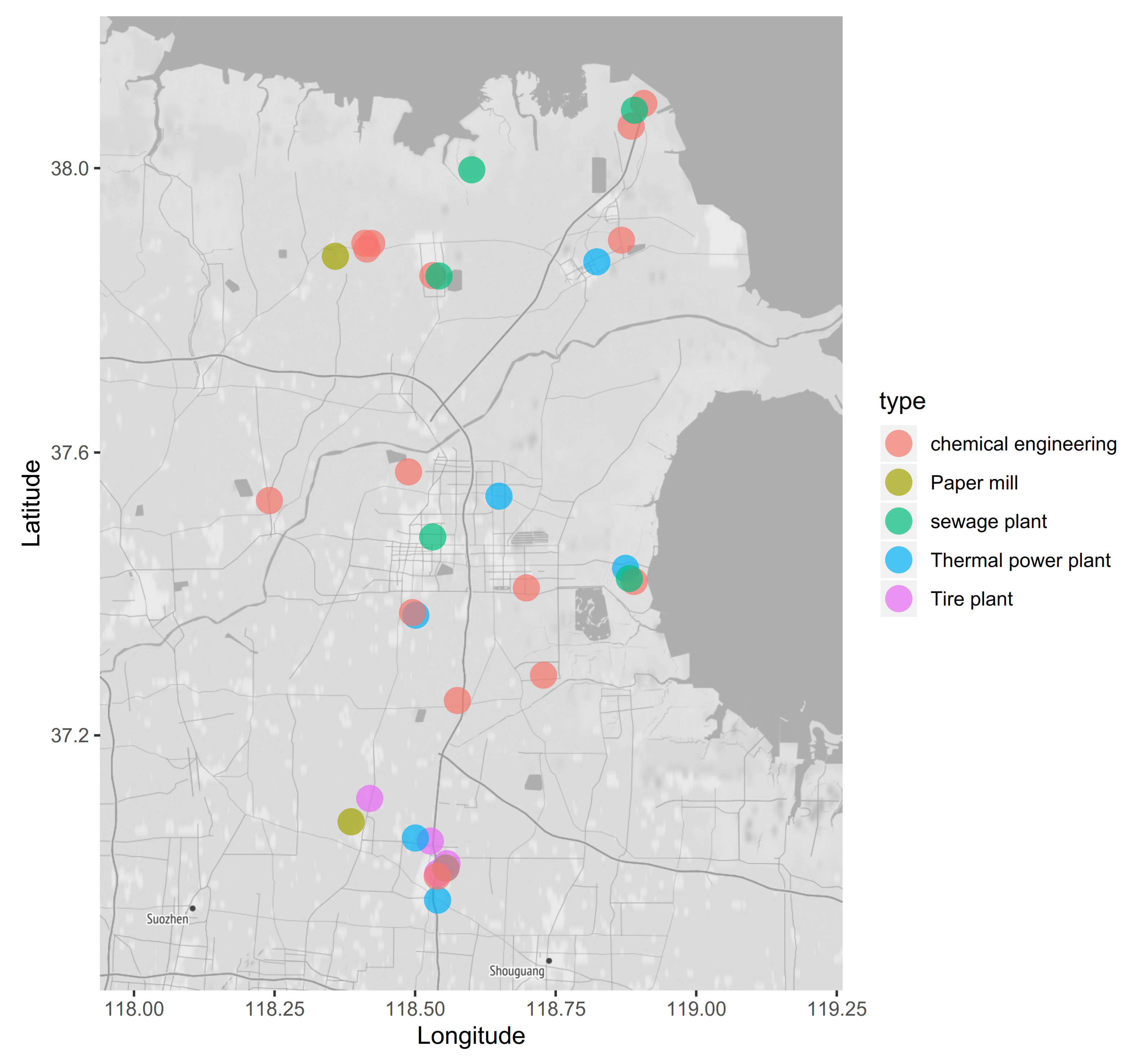
Our study area is located in Shandong Province, China and contains 33 factories as shown in Figure 2. To improve the generalization of analysis results, we select 5 different kinds of factories, which are chemical engineering, paper mill, sewage plant, thermal power plant and tire plant. For each factory, one co-located air quality monitoring system is also installed to measure and record the real-time air quality readings, such as PM 2.5. Now assume that the air quality readings from one factory are missing or wrong and we would like to recover the true air quality measurements from other indirect factors, such as energy consumption values, etc. or from the measurements from surrounding air quality stations. The questions then become that whether it is possible to do the accurate estimation from those indirect factors and what’s the candidate approaches to achieve this goal.
Intuitively, we can recover the air quality readings at a target location from the data of either local or surrounding remote locations:
- Single-location recovery. Given the local factory production data, such as Total energy consumption, Water, Desalted water, Electricity, Steam, Plant-wide fuel, Natural gas, Refinery dry gas, etc., we can find a function to estimate the air pollution levels from those indirect data. Namely, Predicting the missing air quality readings at a target location from those indirect factory production features, which are strongly correlated to the local air pollution emission. We denote this approach as Single-location recovery.
- Multiple-location recovery. We can also borrow the idea from the air quality spatial interpolation research area. Assuming that the air quality readings at a target location are missing, but accurate air quality readings from surrounding locations are available, we can apply the spatial interpolation method to predict the air quality readings from all other available and accurate data. Based on this intuition, we name this method as Multiple-location recovery.
To show the opportunity of recovering the PM 2.5 emission by Single-location recovery.
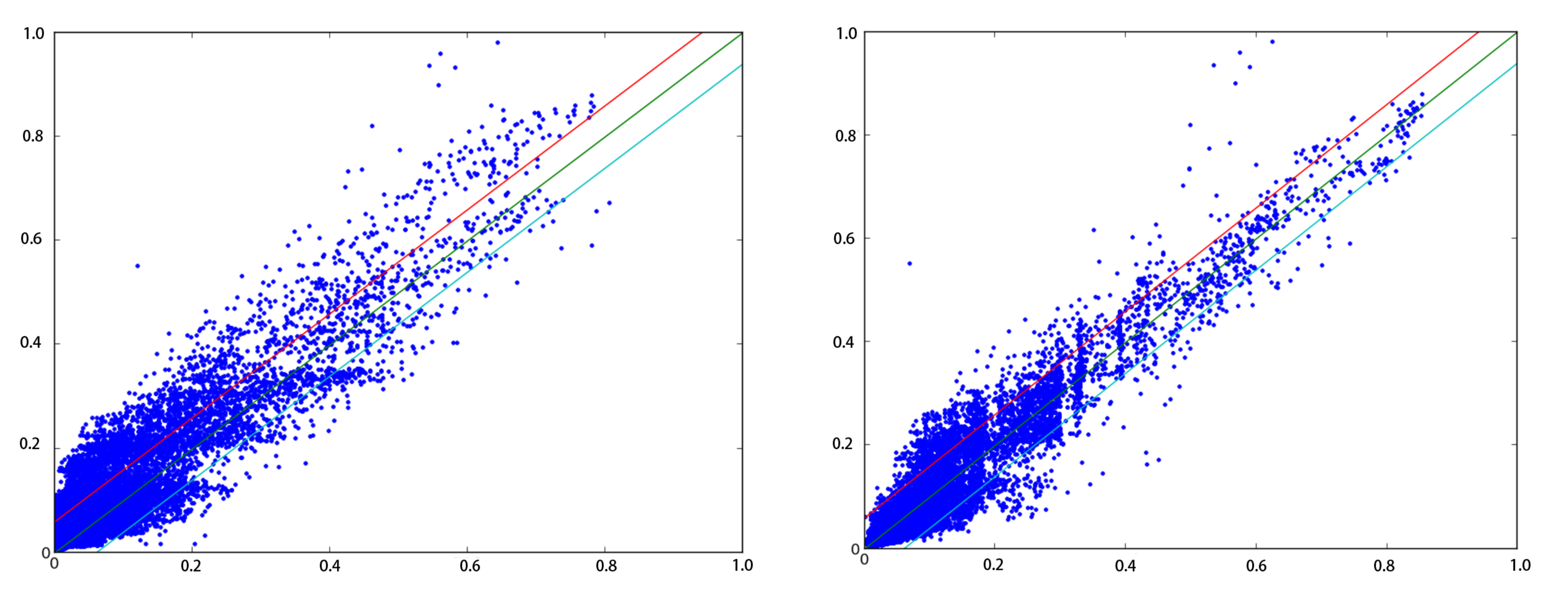
We collect the air quality readings and energy consumptions values over three year, and plot the relationship between them from two different factory types in Figure 3. From the results, we can see that:
- The overall relationship between PM 2.5 and energy consumption is positive-related, namely, more energy consumption leads to more produced air pollution.
- Using single-location indirect features, such as energy consumtion, is not enough to recover the air quality readings accurately and reliably.
If we fit a linear regression model to the data, the between the estimated values and ground truth is above 0.85, which shows that it is possible to recover the air quality readings from those indirect features.
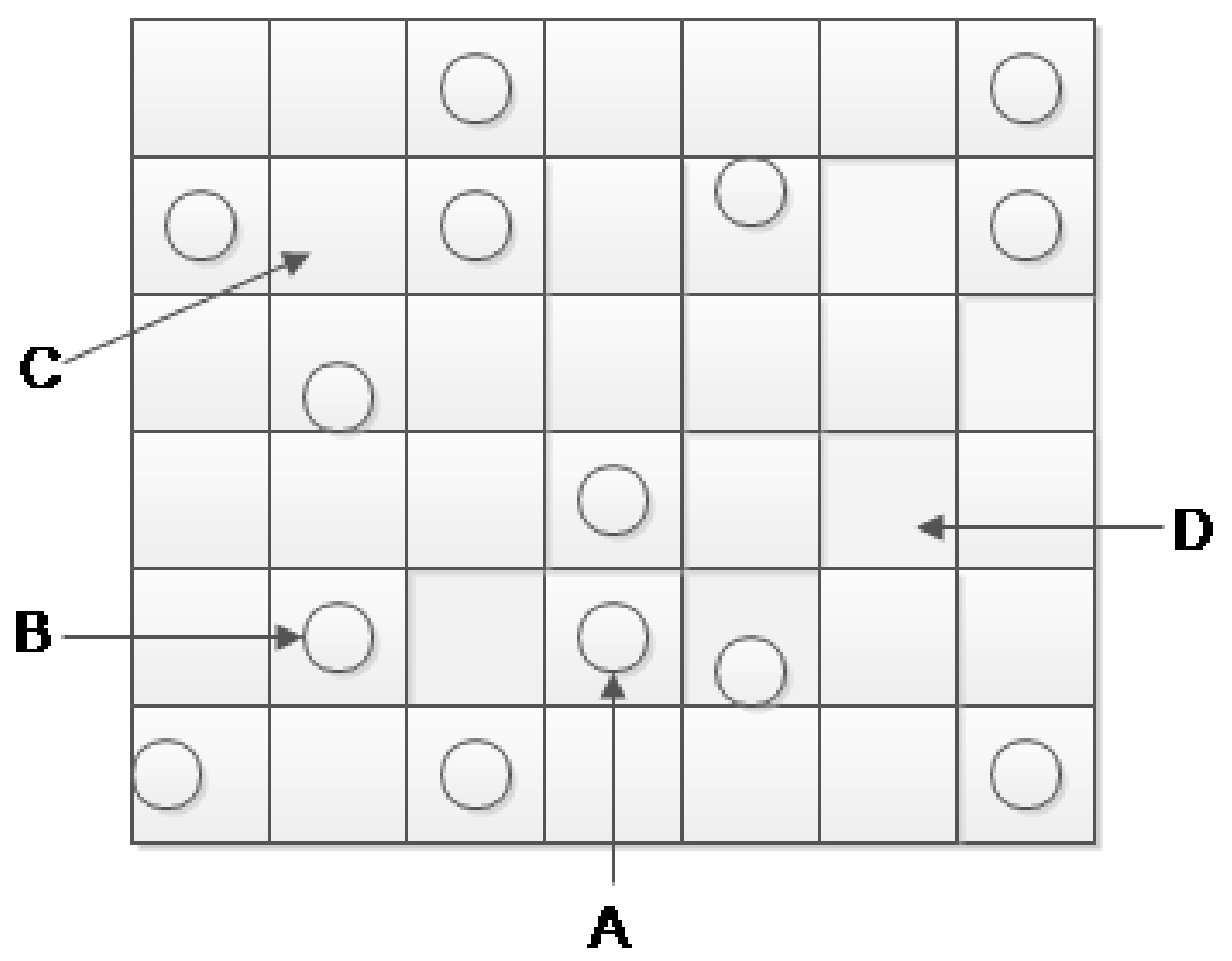
Another possibility of recovering local air quality readings is to predict them from surrounding air quality stations. In order to ensure the authenticity of the selected data, we specially select the government owned air quality monitoring stations as main source of data. Since the factory owners cannot obtain the permission to modify the data collected from government owned air quality monitoring stations, the data integrity is guaranteed. Figure 4 shows the intuition of such Multiple-location recovery. For example, we try to recover the missing ( location C) or wrong readings ( location A or B ) at target locations, we could do the spatial interpolation using surrounding accurate air quality readings. However, if we would like to recover the readings in location D, it’s hard to generate accurate spatial predictions due to the missing surrounding air quality stations, in such scenario, the Single-location recovery may be more accurate than Multiple-location recovery, which motivates that the final optimal approach should be a balanced method between the above two mentioned recovery methods.
4. Methods
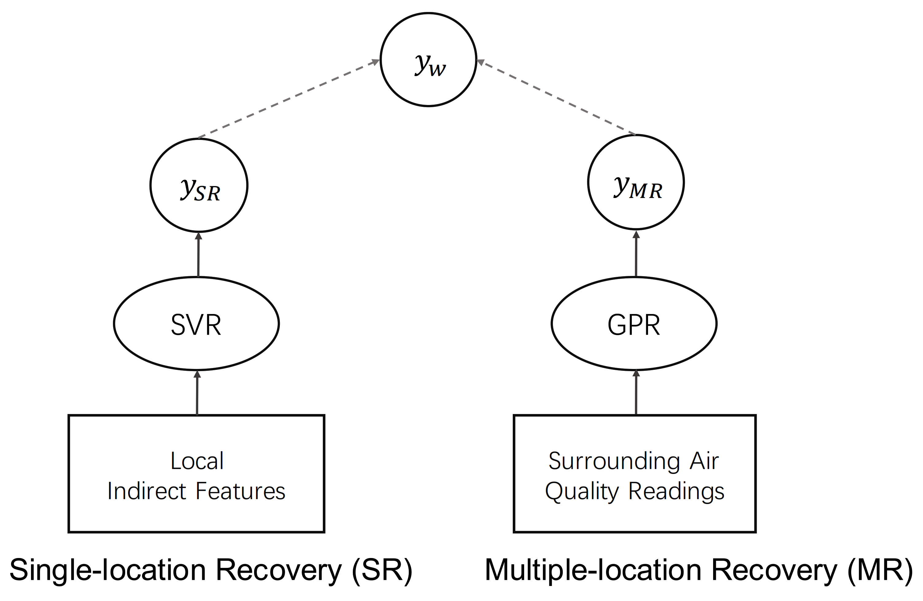
Figure 5 shows the overall framework of our proposed approach. Firstly, to do the Single-location recovery, support vector regression (SVR) is used to learn the relationship between the air quality readings and other indirect features from the factory, its prediction values are referred as . Then, given the surrounding air quality readings, Gaussian Process Regression (GPR) is applied to do the spatial interpolation and predict the air quality readings in our target location, which is Multiple-location recovery. Finally, a weighted mechanism is applied to balance the importance between Single-location recovery and Multiple-location recovery. is then used as the final recovery results of the air quality readings.
In this section, we will first describe our proposed methods for Single-location recovery and multiple-location recovery, then follows the overall combined approach.
4.1. Support Vector Regression for Single-Location Recovery
Given local indirect features (X) of the factory, we could apply Support Vector Regression to estimate the air quality readings (y) from those indirect features.
Support Vector Machine can also be used as a regression method, maintaining all the main features that characterize the algorithm (maximal margin). Although similar logic principle, but unlike the Support Vector Machines (SVM) for two classification problems, Support Vector Regression (SVR) classifies the sample results into one category. For this research, it is very difficult to convert the prediction result into a real number under a variety of data information conditions. Therefore, the tolerance setting in the regression process should be similar to that in SVM. At the same time, this formula design has also greatly increased the complexity. However, due to both the same logic principle, part of the error is negligible. Specially, we try to:
where w is the weights of SVR, with the following constraints:
here is the threadhold. Then, through kernel function operations, the data is divided into high-dimensional feature spaces to achieve linear separation.
In our method, we choose a polynomial kernel due to its simplicity and ability to capture the underlying relationship. More details will be shown in the experiment section.
4.2. Gaussian Process Regression for Multiple-Location Recovery
To further improve the accuracy of the recovered values, apart from the single-location recovery method described in the previous section, we also propose to derive the underlying patterns from surrounding sensor readings. The intuition is that the air quality readings normally have a smooth distribution in an outdoor environment and the air quality value in a target location can be inferred from its surrounding station’s values. Also, this approach is helpful to solve the outlier issues and provide more stable and reliable results. In related works, Gaussian Process (GP) is widely used for the air quality spatial interpolation, which is capable of inferring air quality readings in each grid cell of a monitoring region. In the following section, we will first give a preliminary of the Gaussian Process and then follows the description of how it is used in our problem.
Gaussian Process with random characteristics, which also led to a subset of all random variables must comply with multivariate Gaussian distribution [26,45]. According to the definition, if and fit the following distribution, we say that is drawn from a Gaussian Process with mean function and covariance function .
The simplification can be expressed as:
In our problem, for the kernel function , we find that the squared exponential function as shown below is appropriate for the air quality spatial interpolation problem, so we apply this as our kernel function for Gaussian Process.
where is the meta-information variables of each location. For example, the GPS locations of each location and the Point-of-interest types of each location, etc. Specifically, is the meta-information variables in our target location and x is the meta-information variables in surrounding nearby locations. According to the formula, the kernel function is used to measure the similarity between the target location and all other surrounding locations.Therefore, , regression through Gaussian process can be expressed as
where the error term is that the disturbance variable obeys an independent distribution.
Given the available meta-information variables and air quality readings in all surrounding locations . We can derive the relationship between those variables. Now suppose we have the same meta-information variables in our target location, namely follows the same Gaussian Process distribution, we could infer by computing the posterior predictive distribution as [46]
where is , is , and is . Calculated as follows:
The posterior distribution is shown as
In our problem, each location has the following meta-information variables: the GPS coordinates, humidity, temperature, POI (points of interest). The Gaussian Process Regression model will apply the kernel function to learn the similarity between surrounding locations and our target one, then predict the air quality readings in the target location by using Equation (10), also Equation (11) gives the uncertainty of each prediction.
Generally speaking, the air quality difference between the grids within the monitoring range is not very large [27]. In our scenario, we only use the prediction data with bigger than some threshold (e.g., ). then, the accurate predictions with high certainty are used as the values of Multiple-location recovery.
4.3. Combined Model
Now suppose we get the values from Single-location recovery and from Multiple-location recovery, then for each timestamp i, the optimal recovery reading should be a weighted combination of those two values:
where is a tradeoff valus between 0 and 1, which indicates the importance of those two recovery algorithm. Closer to 1 means that we should pay more attention on the Single-location recovery results, while closer to 0 means that Multiple-location recovery has more accurate and robust results and should be considered.
5. Results
5.1. Dataset and Setup
We collect the air quality readings data and factories’ indirect features data over 3 years from Jan 2016 to Jan 2020 in the research area as shown in Figure 2. Among all the 33 factories, we select 5 of them as test factories and suppose there are missing or mislabeled air quality readings, our goal is to recover the accurate air quality readings based on local indirect features and surrounding air quality readings.
For SVR algorithm, all the input features are described in Table 1, apart from the factory indirect features , we also include the time series features, such as hour of day, day of week, etc. and the weather factors , such as temperature, humidity, etc. Because those DateTime features and weather factors are both important indicators for air pollution emission [47,48,49,50].
The hyper-parameters for our model are selected as follows. For SVR model, we use a polynomial kernel due to its ability to learn complex relationship and set dimension to 2. For Gaussian Process Regression (GPR), we set the covariance parameter to 12. We use Mean Absolute Error (MAE) to evaluate our algorithm. To determine the tradeoff parameter used in Equation (12), we apply the Leave-One-Out Cross-Validation method to evaluate the overall recovery performance by using different . After the evaluation, we set due to its ability to acquire overall highest recovery accuracy for the validation dataset. All our experiments are conducted in a PC with Intel(R) Core(TM) i7-7600U CPU and all the code is implemented in python.
5.2. Single-Location Recovery
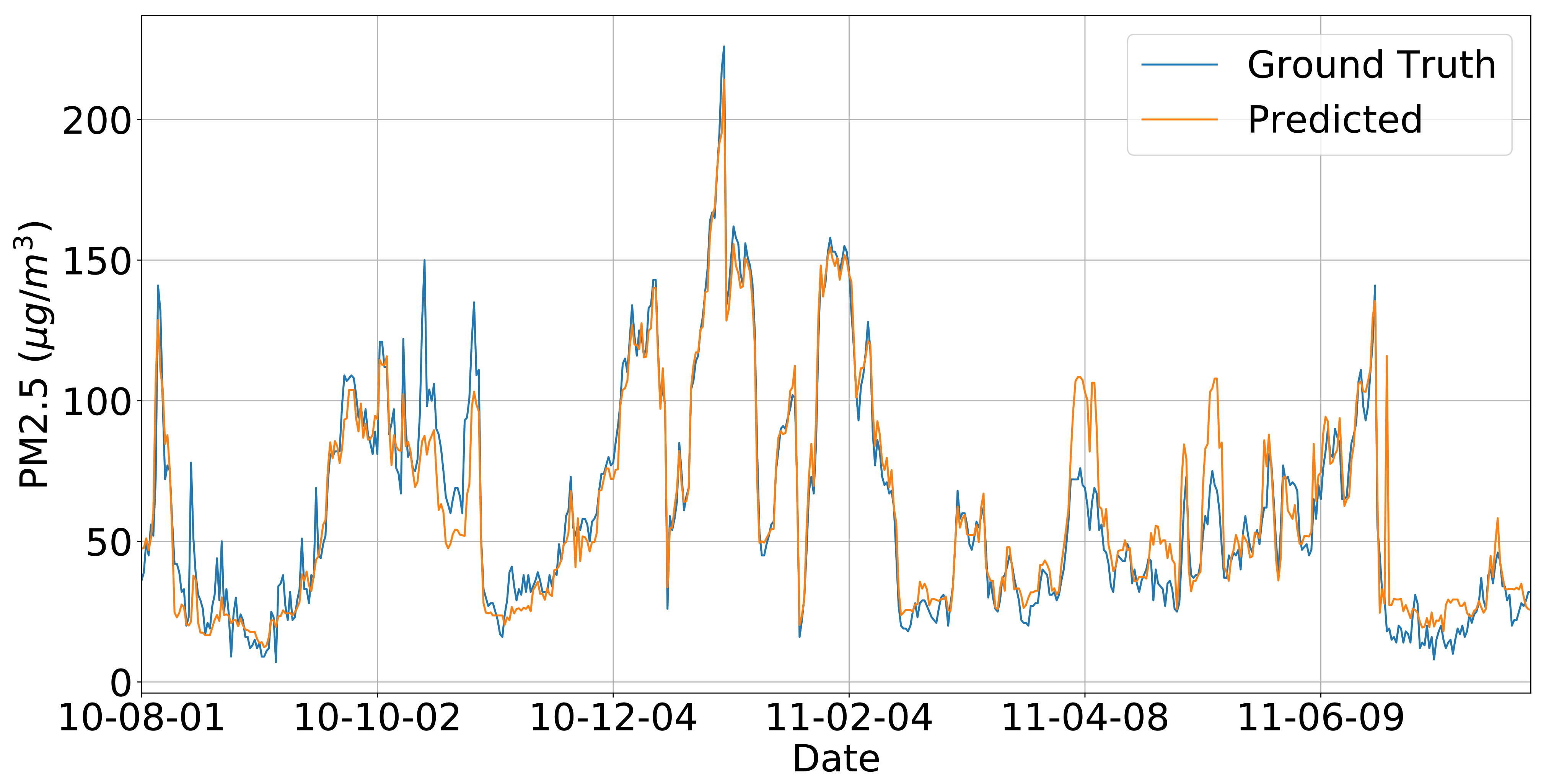
Figure 6 shows the SVR prediction results, the predicted values fit quite well with the ground truth air quality monitoring measurements, which means that the SVR model could successfully recover the air quality readings from other indirect features.
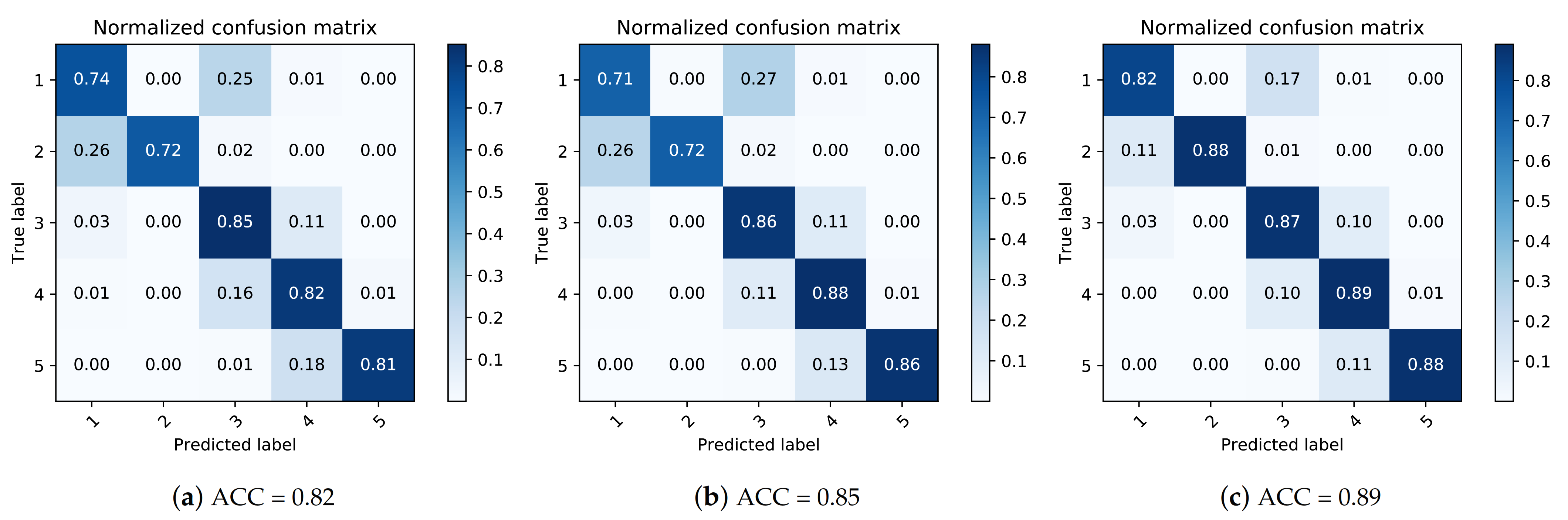
In order to evaluate the effectiveness and importance of all the features used in SVR model, we sequentially add factory indirect features, DateTime features and meteorological features, and compare the prediction results using confusion matrices as shown in Figure 7. The results show that the prediction accuracy is by using only the factory indirect features. After adding DateTime features and weather features to the SVR model sequentially, the prediction accuracy improves to and , respectively.
The above results show that: (i) The SVR model is promising to recover the missing or mislabeled air quality readings from other indirect factors; (ii) Apart from factory indirect factors, such as energy consumption, etc. Datetime features and weather features are also important indicators for accurate predictions.
5.3. Multiple-Location Recover
As we have shown in the previous section, Single-location recovery is capable to predict the air quality readings accurately from indirect factors. However, in some cases, those indirect features may be missing for some factories, which makes it impossible to recover the air quality readings accurately and reliably anymore.
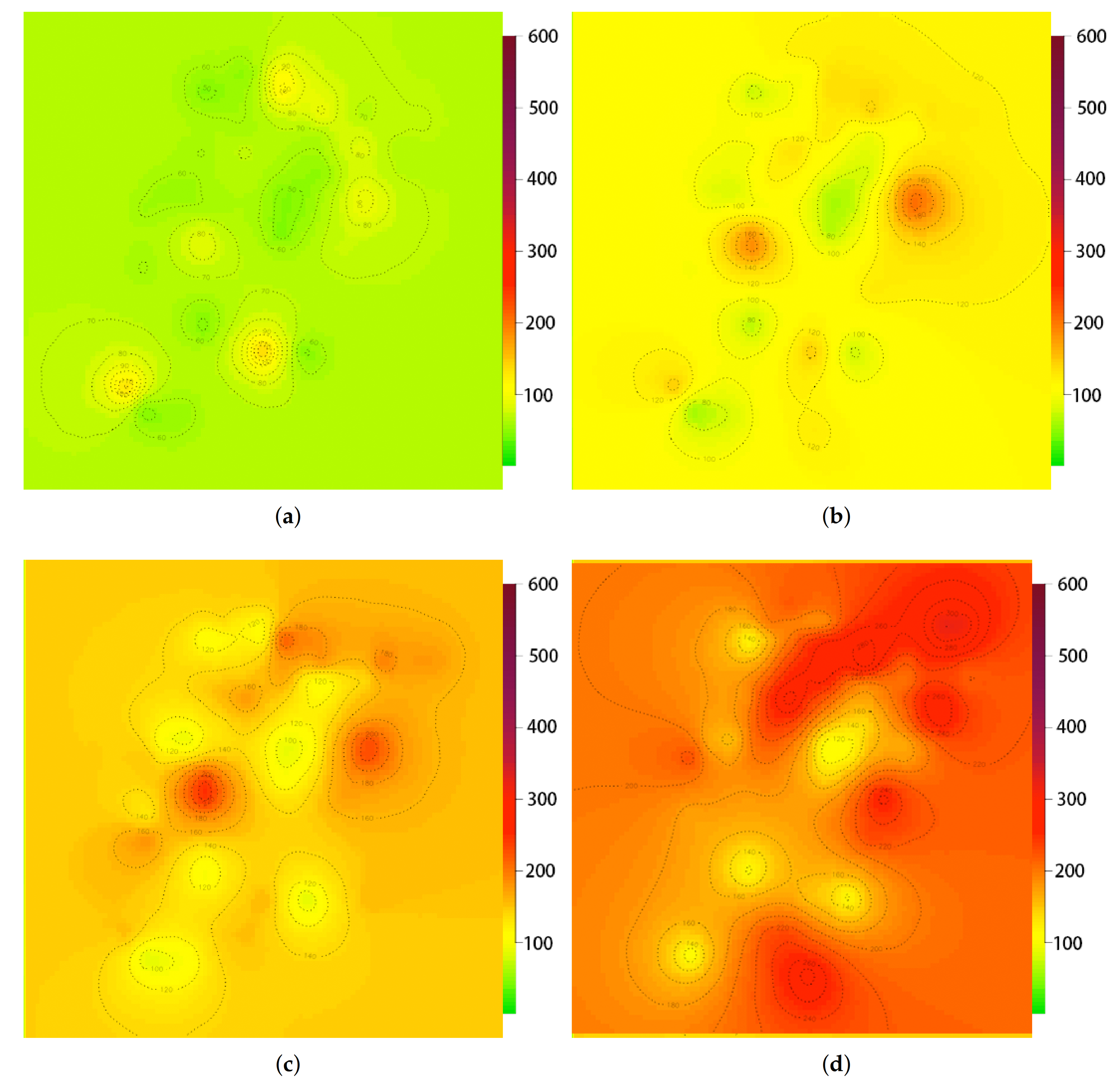
To solve this challenge, we use a widely used spatial interpolation method called GPR to generate air quality maps at each timestamp using all the available air quality readings and recover values at unknown locations. Figure 8 shows the examples of generated air quality maps in different pollution levels. Specifically, Figure 8a demonstrates that the most of the PM 2.5 density is below 100 μg/m for the mild pollution. And, the Figure 8d depicts that the PM 2.5 density is between 300 to 400 μg/m for the severe pollution level. We can see that the spatial prediction is smoothing and promising to recover accurate air quality readings for those unknown locations.
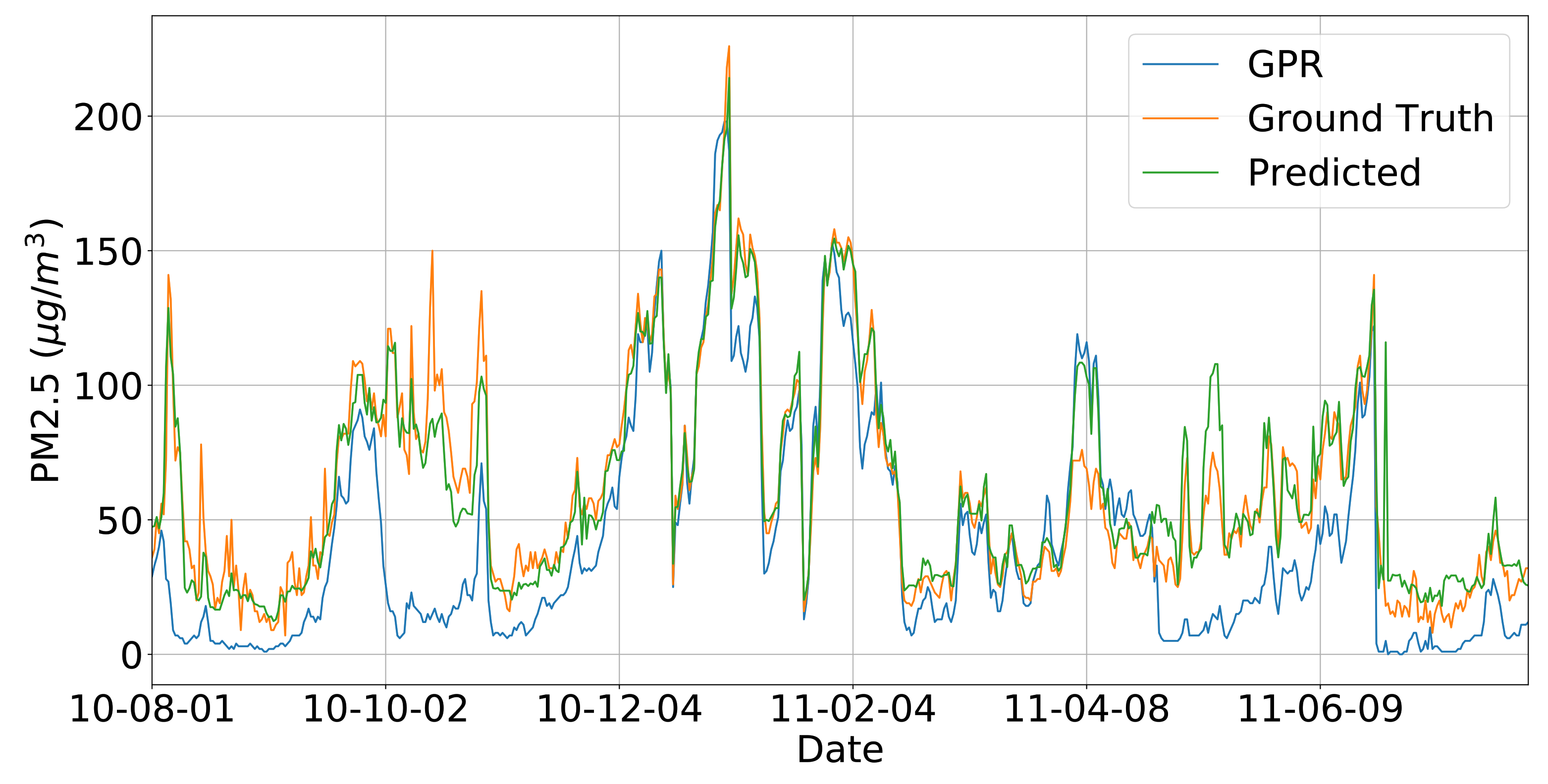
Figure 9 shows the predicted time series results by using different methods: SVR (if all indirect features are available) or GPR. From the comparison with the ground truth air quality readings, we can conclude that: (i) SVR is more accurate compared with GPR method if all indirect features are available and can be used as inputs to the model; (ii) In extreme cases, such as missing indirect features, GPR is also acceptable to be used as an indicator for the air quality concentrations in our target locations.
5.4. Impact of Season
Our experiment is performed to estimate the air pollutant emission over a year. The results shown in Figure 6 and Figure 9 reflect the seasonal change of the estimated results and the ground truth. That is PM 2.5 increases from autumn and the highest value in the winter because of two reasons: (i), most of the factories receive more orders prior to the Lunar new year eve and therefore their energy consumption and the corresponding air pollutant emission increase from automn to winter. (ii), the factories burn more coal to heat the factory in the winter, thereby emitting more air polutants. For spring and summer, the factories usually receive less number of orders and therefore emit less ait pollutant.
5.5. Overall Recovery
Table 2 shows the overall evaluation results using a single component or the weighted combination of Single-location recovery and Multiple-location recovery. From the results, we can see that, for each single component method, SVR or GPR both have accurate predictions and unpromising prediction results, however, after combining them together with a weighted factor, the overall Mean Absolute Error (MAE) is below 9, which is small and can be used in other related research areas [51]. We also compare our method with state-of-art PM2.5 spatial interpolation method AirCloud [27], which also use GPR as the spatial interpolation method, but with a default setting. The results show that our method, which fine-tunes the parameters instead of using the default ones, outperforms AirCloud by , ,, and , showing its ability to improve the data accuracy and reliability in single-location.
Also, we compared the prediction results from 5 different factory types. The results show that our proposed model is robust enough to generate reasonable recovery air quality readings in different scenarios and promising to be used in real practice.
6. Discussion and Suggestion
With the rapid development of Internet technology, e-government has long become an important means for Chinese government departments to perform their functions. From information collection to data archiving, various departments have established electronic databases with various types and complete information. For air pollution monitoring, although these databases have improved work efficiency, due to the independence of departmental supervision, a large number of related data (such as energy consumption data, material data, etc.) have not been thoroughly explored. These data are an important basis for screening factory exhaust emissions. Under such circumstances, relevant government departments (such as the Development and Reform Commission, the Bureau of Industry and Information Technology, and the Environment Bureau, etc.) should establish a full-time department for mining the relationship between various data and pollutant emissions on the basis of the existing big data center. The specific plan is as follows:
- Prepare a multi-departmental collaborative implementation plan for related information such as supporting equipment, information processing, information technology, human resources, and implementation procedures.
- Establish a multi-source database covering basic enterprise information, industrial chain information, and enterprise emergency environmental accident cases, based on which the factories are classified and managed to improve the quality and efficiency of exhaust emission supervision.
- Adjust pollutant discharge management institutions according to the nature of the industry, implement refined and standardized management of pollution discharge surveys, inspections and assessments, and discharge volume verification in key industries, generate discharge data supervision reports on schedule, and conduct dynamic management and evaluation of supervision content.
- Establish a data sharing platform among multiple government departments such as the Environment Bureau, the Taxation Bureau, and the Bureau of Industry and Information Technology to break the phenomenon of “information islands” and “data conflicts”, and realize real-time sharing of data related to surrounding monitoring point sources and corporate pollution.
Up to now, the environmental department has only installed pollutant emission monitoring equipment in large-scale enterprises, and has not involved small and micro enterprises. The monitoring network that is not tight enough cannot achieve comprehensive monitoring of pollutant emission point sources. Therefore, how to increase the layout of pollutant monitoring equipment and form an effective data transmission network is an engineering problem that needs to be solved urgently. At the same time, engineers have to think about how to capture, clean and calculate data in a timely and accurate manner in the face of massive cloud data after forming a pollutant monitoring network.
As the paper [52] suggests, the PM 2.5 concentration is highly related with the local economy. Specifically, the price of the energy source varies with the different types. For instance, the factories using the renewable energy, including wind and tide, often get subsidies from local governments while factories using fossil energy have to pay more according to the local governments’ policies [53]. Nevertheless, such penalty policies cannot contribute to reducing the PM 2.5 emission. As [53] describes, coal consumption, which is the main cause of PM 2.5, grew by 214% from 2000 to 2012, regardless of the strict price control imposed by the government. This observation shows the difficulty of reducing the consumption of fossil energy by controlling the price, further indicating the challenges of controlling PM 2.5 emission. Therefore, we would like to leave the research of how industries adapt their consumption according to energy price and thus affect PM 2.5 concentrations to the future work.
7. Conclusions
This paper introduces a novel approach to monitor the air pollutant emission (PM 2.5) taking both a factory’s energy consumption and government’s air quality readings into account. Firstly, we use a primary study to show the possibility and challenges of using the above-mentioned features to accurately estimate the air quality readings. Then, to solve the challenges, we proposed Single-location recovery and Multiple-location recovery algorithm. Support Vector Regression (SVR) is applied to recover the missing or mislabeled air quality values from indirect factors in Single-location recovery model, and Gaussian Process Regression (GPR) is used to do the spatial interpolation and predict the air quality readings in the target location in Multiple-location recovery. Finally, a combined model is proposed to combine both models and do a meaningful tradeoff between them.
The experiments on SVR performance show that SVR is powerful enough to produce accurate prediction results given all indirect factory features, Datetime features, and weather features. We also evaluate the feature importance on the overall prediction accuracy by sequentially adding them to the model. Then, we evaluate the recovery performance by using GPR model under the missing indirect factory features scenario, the results show that GPR model is also promising to generate accurate air quality maps and give reasonable recovered air quality readings. Finally, the overall weighted scheme is evaluated on 5 different kinds of factory types, the results show that our proposed approach is accurate and robust to be applied to different scenarios and used in practice.
Author Contributions
X.G. conceived and designed the research framework; H.W. wrote the paper and performed the experiments and analyzed the data. All authors have read and agreed to the published version of the manuscript.
Funding
This research is supported by The National Social Science Fund of China (Grant NO. 20BTJ060), And Shandong Provincial Natural Science Foundation, China (Grant NO. ZR2020MG065).
Institutional Review Board Statement
Not applicable.
Informed Consent Statement
Not applicable.
Data Availability Statement
Data is available on request from the corresponding author of the manuscript.
Acknowledgments
We sincerely thank the anonymous editors and reviewers for their valuable comments and suggestions. We also appreciate Phoenixlab for the efforts in revising this paper.
Conflicts of Interest
The authors declare no conflict of interest.
References
- Boretti, A.; Rosa, L. Reassessing the projections of the world water development report. NPJ Clean Water 2019, 2, 1–6. [Google Scholar] [CrossRef]
- Li, X.; Jin, L.; Kan, H. Air pollution: A global problem needs local fixes. Nature 2019, 570, 437–439. [Google Scholar] [CrossRef] [Green Version]
- Boamah, K.B.; Du, J.; Boamah, A.J.; Appiah, K. A study on the causal effect of urban population growth and international trade on environmental pollution: Evidence from China. Environ. Sci. Pollut. Res. 2017, 25, 5862–5874. [Google Scholar] [CrossRef] [PubMed]
- He, P.; Sun, Y.; Shen, H.; Jian, J.; Yu, Z. Does Environmental Tax Affect Energy Efficiency? An Empirical Study of Energy Efficiency in OECD Countries Based on DEA and Logit Model. Sustainability 2019, 11, 3792. [Google Scholar] [CrossRef] [Green Version]
- Krass, D.; Nedorezov, T.; Ovchinnikov, A. Environmental taxes and the choice of green technology. Prod. Oper. Manag. 2013, 22, 1035–1055. [Google Scholar] [CrossRef]
- Kemp, R.; Pontoglio, S. The innovation effects of environmental policy instruments—A typical case of the blind men and the elephant? Ecol. Econ. 2011, 72, 28–36. [Google Scholar] [CrossRef]
- Choi, T. Local sourcing and fashion quick response system: The impacts of carbon footprint tax. Transp. Res. Part E Logist. Transp. Rev. 2013, 55, 43–54. [Google Scholar] [CrossRef]
- Onofrei, M.; Vintilă, G.; Dascalu, E.D.; Roman, A.; Firtescu, B.N. The impact of environmental tax reform on greenhouse gas emissions: Empirical evidence from European countries. Environ. Eng. Manag. J. 2017, 16, 2843–2849. [Google Scholar] [CrossRef]
- Agnolucci, P. The effect of the German and British environmental taxation reforms: A simple assessment. Energy Policy 2009, 37, 3043–3051. [Google Scholar] [CrossRef]
- Gulia, S.; Khanna, I.; Shukla, K.; Khare, M. Ambient air pollutant monitoring and analysis protocol for low and middle income countries: An element of comprehensive urban air quality management framework. Atmos. Environ. 2019, 222, 117120. [Google Scholar] [CrossRef]
- Chalabi, Z.; Milojevic, A.; Doherty, R.M.; Stevenson, D.S.; MacKenzie, I.A.; Milner, J.; Vieno, M.; Williams, M.; Wilkinson, P. Applying air pollution modelling within a multi-criteria decision analysis framework to evaluate UK air quality policies. Atmos. Environ. 2017, 167, 466–475. [Google Scholar] [CrossRef]
- Boyce, J.K.; Pastor, M. Clearing the air: Incorporating air quality and environmental justice into climate policy. Clim. Chang. 2013, 120, 801–814. [Google Scholar] [CrossRef]
- Cai, H.; Xie, S. Traffic-related air pollution modeling during the 2008 beijing olympic games: The effects of an odd-even day traffic restriction scheme. Sci. Total Environ. 2011, 409, 1935–1948. [Google Scholar] [CrossRef] [PubMed]
- Gao, J.; Yuan, Z.; Liu, X.; Xia, X.; Huang, X.; Dong, Z. Improving air pollution control policy in China—A perspective based on cost–benefit analysis. Sci. Total Environ. 2016, 543, 307–314. [Google Scholar] [CrossRef]
- Yang, S.; Chen, B.; Wakeel, M.; Hayat, T.; Alsaedi, A.; Ahmad, B. PM2.5 footprint of household energy consumption. Appl. Energy 2018, 227, 375–383. [Google Scholar] [CrossRef]
- Wang, S.; Kim, S.M.; He, T. Symbol-level cross-technology communication via payload encoding. In Proceedings of the IEEE 38th International Conference on Distributed Computing Systems (ICDCS), Vienna, Austria, 2–5 July 2018; pp. 500–510. [Google Scholar]
- Chae, Y.; Wang, S.; Kim, S.M. Exploiting wifi guard band for safeguarded zigbee. In Proceedings of the 16th ACM Conference on Embedded Networked Sensor Systems, Shenzhen, China, 4–7 November 2018; pp. 172–184. [Google Scholar]
- Li, K.; Wang, S. Electric vehicle charging station deployment for minimizing construction cost. In Proceedings of the International Conference on Big Data Analytics and Knowledge Discovery, Lyon, France, 28–31 August 2017; pp. 471–485. [Google Scholar]
- Jeong, W.; Jung, J.; Wang, Y.; Wang, S.; Yang, S.; Yan, Q.; Yi, Y.; Kim, S.M. SDR receiver using commodity wifi via physical-layer signal reconstruction. In Proceedings of the 26th Annual International Conference on Mobile Computing and Networking, London, UK, 25–26 March 2020; pp. 1–14. [Google Scholar]
- Ji, Z.; Wang, S. Online truthfully incentive mechanisms with budget constraint for multiple overlapped tasks crowdsourced sensing. In Proceedings of the 2017 IEEE 2nd Information Technology, Networking, Electronic and Automation Control Conference (ITNEC), Chengdu, China, 15–17 December 2017; pp. 999–1003. [Google Scholar]
- Eronat, A.H.; Bengil, F.; Neser, G. Shipping and ship recycling related oil pollution detection in candarh bay (Turkey) using satellite monitoring. Ocean. Eng. 2019, 187, 106157.1–106157.8. [Google Scholar] [CrossRef]
- Aliyu, Y.A.; Botai, J.O. Appraising city-scale pollution monitoring capabilities of multi-satellite datasets using portable pollutant monitors. Atmos. Environ. 2018, 179, 239–249. [Google Scholar] [CrossRef] [Green Version]
- Khaki, M.; Awange, J. The application of multi-mission satellite data assimilation for studying water storage changes over south america. Sci. Total Environ. 2018, 647, 1557–1572. [Google Scholar] [CrossRef]
- Li, J.; Zhang, H.; Chaoa, C.Y.; Chien, C.H.; Biswas, P. Integrating low-cost air quality sensor networks with fixed and satellite monitoring systems to study ground-level pm2.5. Atmos. Environ. 2020, 223, 117293. [Google Scholar] [CrossRef]
- Dewinter, J.L.; Brown, S.G.; Seagram, A.F.; Landsberg, K.; Eisinger, D.S. A national-scale review of air pollutant concentrations measured in the u.s. near-road monitoring network during 2014 and 2015. Atmos. Environ. 2018, 183, 94–105. [Google Scholar] [CrossRef]
- Cheng, Y.; Li, X.; Li, Z.; Jiang, S.; Jiang, X. Fine-Grained Air Quality Monitoring Based on Gaussian Process Regression. In Proceedings of the International Conference on Neural Information Processing, Kuching, Malaysia, 3–6 November 2014. [Google Scholar]
- Cheng, Y.; Li, X.; Li, Z.; Jiang, S.; Li, Y.; Jia, J.; Jiang, X. AirCloud: A cloud-based air-quality monitoring system for everyone. In Proceedings of the 12th ACM Conference on Embedded Network Sensor Systems, Memphis, Tennessee, 3–6 November 2014; pp. 251–265. [Google Scholar]
- Gao, M.; Beig, G.; Song, S.; Zhang, H.; Hu, J.; Ying, Q.; McElroy, M.B. The impact of power generation emissions on ambient PM2.5 pollution and human health in China and India. Environ. Int. 2018, 121, 250–259. [Google Scholar] [CrossRef]
- Fahimnia, B.; Sarkis, J.; Choudhary, A.; Eshragh, A. Tactical supply chain planning under a carbon tax policy scheme: A case study. Int. J. Prod. Econ. 2015, 164, 206–215. [Google Scholar] [CrossRef] [Green Version]
- Hariga, M.; As’ ad, R.; Shamayleh, A. Integrated economic and environmental models for a multi stage cold supply chain under carbon tax regulation. J. Clean. Prod. 2017, 166, 1357–1371. [Google Scholar] [CrossRef]
- Chen, Y.J.; Sheu, J. Environmental-regulation pricing strategies for green supply chain management. Transp. Res. Part -Logist. Transp. Rev. 2009, 45, 667–677. [Google Scholar] [CrossRef] [Green Version]
- Keoleian, G.A.; Volk, T.A. Renewable energy from willow biomass crops: Life cycle energy, environmental and economic performance. Crit. Rev. Plant Sci. 2005, 24, 385–406. [Google Scholar] [CrossRef]
- Bjorklund, A.E.; Finnveden, G. Life cycle assessment of a national policy proposal—The case of a Swedish waste incineration tax. Waste Manag. 2007, 27, 1046–1058. [Google Scholar] [CrossRef] [PubMed]
- Wu, K.; Feng, Y.; Yu, G.; Liu, L.; Li, J.; Xiong, Y.; Li, F. Development of an imaging gas correlation spectrometry based mid-infrared camera for two-dimensional mapping of CO in vehicle exhausts. Opt. Express 2018, 26, 8239–8251. [Google Scholar] [CrossRef]
- Li, T.; Winnel, M.; Lin, H.; Panther, J.; Liu, C.; O’Halloran, R.; Zhao, H. A reliable sewage quality abnormal event monitoring system. Water Res. 2017, 121, 248–257. [Google Scholar] [CrossRef] [PubMed]
- Gallardo-Gonzalez, J.; Baraket, A.; Boudjaoui, S.; Metzner, T.; Hauser, F.; Rößler, T.; Bausells, J. A fully integrated passive microfluidic Lab-on-a-Chip for real-time electrochemical detection of ammonium: Sewage applications. Sci. Total Environ. 2019, 653, 1223–1230. [Google Scholar] [CrossRef]
- Marchant, C.; Leiva, V.; Christakos, G.; Cavieres, M.F. Monitoring urban environmental pollution by bivariate control charts: New methodology and case study in Santiago, Chile. Environmetrics 2019, 30, e2551. [Google Scholar] [CrossRef]
- Wang, S.; Jeong, W.; Jung, J.; Kim, S.M. X-MIMO: Cross-technology multi-user MIMO. In Proceedings of the 18th Conference on Embedded Networked Sensor Systems, Yokohama, Japan, 16 November 2020; pp. 218–231. [Google Scholar]
- McKercher, G.R.; Vanos, J.K. Low-cost mobile air pollution monitoring in urban environments: A pilot study in Lubbock, Texas. Environ. Technol. 2018, 39, 1505–1514. [Google Scholar] [CrossRef]
- Hswen, Y.; Qin, Q.; Brownstein, J.S.; Hawkins, J.B. Feasibility of using social media to monitor outdoor air pollution in London, England. Prev. Med. 2019, 121, 86–93. [Google Scholar] [CrossRef] [PubMed]
- Pourshahabi, S.; Rakhshandehroo, G.; Talebbeydokhti, N.; Nikoo, M.R.; Masoumi, F. Handling Uncertainty in Optimal Design of Reservoir Water Quality Monitoring Systems. Environ. Pollut. 2020, 266, 115211. [Google Scholar] [CrossRef]
- Martin, C.; Parkes, S.; Zhang, Q.; Zhang, X.; McCabe, M.F.; Duarte, C.M. Use of unmanned aerial vehicles for efficient beach litter monitoring. Mar. Pollut. Bull. 2018, 131, 662–673. [Google Scholar] [CrossRef] [PubMed] [Green Version]
- Bian, X.; Li, X.; Qi, P.; Chi, Z.; Ye, R.; Lu, S.; Cai, Y. Quantitative design and analysis of marine environmental monitoring networks in coastal waters of China. Mar. Pollut. Bull. 2019, 143, 144–151. [Google Scholar] [CrossRef]
- Ripoll, A.; Viana, M.; Padrosa, M.; Querol, X.; Minutolo, A.; Hou, K.M.; García-Vidal, J. Testing the performance of sensors for ozone pollution monitoring in a citizen science approach. Sci. Total Environ. 2018, 651, 1166–1179. [Google Scholar] [CrossRef]
- Rasmussen, C.E. Gaussian processes in machine learning. In Summer School on Machine Learning; Bousquet, O., von Luxburg, U., Rätsch, G., Eds.; Springer: Berlin, Germany, 2003; pp. 63–71. [Google Scholar]
- Murphy, K.P. Machine learning: A probabilistic perspective. In Machine Learning: A Probabilistic Perspective; Springer: Boston, MA, USA, 2012. [Google Scholar]
- Cheng, Y.; He, X.; Zhou, Z.; Thiele, L. MapTransfer: Urban Air Quality Map Generation for Downscaled Sensor Deployments. In Proceedings of the 2020 IEEE/ACM Fifth International Conference on Internet-of-Things Design and Implementation (IoTDI), Sydney, Australia, 21–24 April 2020; pp. 14–26. [Google Scholar]
- Cheng, Y.; Li, X.; Li, Y. Finding dynamic co-evolving zones in spatial-temporal time series data. In Proceedings of the Joint European Conference on Machine Learning and Knowledge Discovery in Databases, Riva del Garda, Italy, 19–23 September 2016; pp. 129–144. [Google Scholar]
- Cheng, Y.; He, X.; Zhou, Z.; Thiele, L. Ict: In-field calibration transfer for air quality sensor deployments. In Proceedings of the ACM on Interactive, Mobile, Wearable and Ubiquitous Technologies, Austin, TX, USA, 9–13 November 2019; pp. 1–19. [Google Scholar]
- Einsiedler, J.; Cheng, Y.; Papst, F.; Saukh, O. Interpretable and Transferable Models to Understand the Impact of Lockdown Measures on Local Air Quality. arXiv 2020, arXiv:2011.10144. [Google Scholar]
- Bellinger, C.; Mohomed Jabbar, M.S.; Zaïane, O.; Osornio-Vargas, A. A systematic review of data mining and machine learning for air pollution epidemiology. BMC Public Health 2017, 17, 907. [Google Scholar] [CrossRef] [Green Version]
- Chen, J.; Zhou, C.; Wang, S.; Li, S. Impacts of energy consumption structure, energy intensity, economic growth, urbanization on PM2. 5 concentrations in countries globally. Apply Energy 2018, 230, 94–105. [Google Scholar] [CrossRef]
- Xie, X.; Ai, H.; Deng, Z. Impacts of the scattered coal consumption on PM2.5 pollution in China. J. Clean. Prod. 2020, 245, 118922. [Google Scholar] [CrossRef]
Figure 1.
An illustration of the factory with the continuous emissions monitoring system installed to monitor the status of emission of pollutants.
Figure 1.
An illustration of the factory with the continuous emissions monitoring system installed to monitor the status of emission of pollutants.

Figure 2.
Factories locations in our study area.

Figure 3.
The relationship between normalized PM2.5 and the energy consumption from two factories.

Figure 4.
Illustration of the spatial pattern between current location and surround locations where monitoring stations are marked in the circle and four represented locations from A to D are selected.
Figure 4.
Illustration of the spatial pattern between current location and surround locations where monitoring stations are marked in the circle and four represented locations from A to D are selected.

Figure 5.
The overall framework.

Figure 6.
The SVR prediction of PM 2.5 from August 2010 to July 2011.

Figure 7.
Confusion matrices of prediction accuracy of is illustrated here. Specifically, (a) shows the result of using only indirect features , (b) also takes the datetime features into account, and (c) considers indirect features , the datetime features , and the meteorological features .
Figure 7.
Confusion matrices of prediction accuracy of is illustrated here. Specifically, (a) shows the result of using only indirect features , (b) also takes the datetime features into account, and (c) considers indirect features , the datetime features , and the meteorological features .

Figure 8.
Gaussian Process Regression of PM 2.5 (μg/m) under different pollution levels. Specifically, (a–d) show the regression results under the PM 2.5 ≤ 100 μg/m, 100–200 μg/m, 200–300 μg/m, and 300–400 μg/m respectively while (a) represents the mild pollution and (d) represents the severe pollution.

Figure 9.
The GP Predictionof PM 2.5 from August 2010 to July 2011.


Table 1.
Features for SVR.
| Categories | Features | No. |
|---|---|---|
| hour of day, day of week, month and is Holiday | 4 | |
| temperature, humidity, pressure, wind speed and wind power | 5 | |
| Factory Indirect Features: Total energy consumption, Water, Desalted water, Electric, Steam, Plant-wide fuel, Natural gas, Refinery dry gas, etc. | 20 |
Table 2.
Overall results MAE (μg/m).
| Chemical Engineering | Paper Mill | Sewage Plant | Thermal Power Plant | Tire Plant | |
|---|---|---|---|---|---|
| SVR | 8.12 | 9.43 | 10.14 | 9.22 | 10.22 |
| GPR | 12.15 | 14.33 | 9.23 | 10.21 | 9.21 |
| AirCloud | 12.83 | 14.52 | 9.31 | 10.62 | 9.32 |
| Combined | 7.21 | 8.64 | 8.34 | 7.29 | 8.09 |
Publisher’s Note: MDPI stays neutral with regard to jurisdictional claims in published maps and institutional affiliations. |
© 2021 by the authors. Licensee MDPI, Basel, Switzerland. This article is an open access article distributed under the terms and conditions of the Creative Commons Attribution (CC BY) license (http://creativecommons.org/licenses/by/4.0/).
Share and Cite
MDPI and ACS Style
Wu, H.; Gao, X. Multimodal Data Based Regression to Monitor Air Pollutant Emission in Factories. Sustainability 2021, 13, 2663. https://0-doi-org.brum.beds.ac.uk/10.3390/su13052663
AMA Style
Wu H, Gao X. Multimodal Data Based Regression to Monitor Air Pollutant Emission in Factories. Sustainability. 2021; 13(5):2663. https://0-doi-org.brum.beds.ac.uk/10.3390/su13052663
Chicago/Turabian StyleWu, Hao, and Xinwei Gao. 2021. "Multimodal Data Based Regression to Monitor Air Pollutant Emission in Factories" Sustainability 13, no. 5: 2663. https://0-doi-org.brum.beds.ac.uk/10.3390/su13052663
Note that from the first issue of 2016, this journal uses article numbers instead of page numbers. See further details here.