
Land Use Dynamics and Optimization from 2000 to 2020 in East Guangdong Province, China
by
 ,
,
Yong Lai
1,2,3 ,
,
Guangqing Huang
2,3,*, 
Shengzhong Chen
2,
Shaotao Lin
2,
Wenjun Lin
2 and
Jixin Lyu
2 1
Guangzhou Institute of Geochemistry, Chinese Academy of Sciences, Guangzhou 510640, China
2
Key Lab of Guangdong for Utilization of Remote Sensing and Geographical Information System, Guangdong Open Laboratory of Geospatial Information Technology and Application, Guangzhou Institute of Geography, Guangdong Academy of Sciences, Guangzhou 510070, China
3
University of Chinese Academy of Sciences, Beijing 100049, China
*
Author to whom correspondence should be addressed.
Sustainability 2021, 13(6), 3473; https://0-doi-org.brum.beds.ac.uk/10.3390/su13063473
Submission received: 17 February 2021
/
Revised: 9 March 2021
/
Accepted: 17 March 2021
/
Published: 21 March 2021
(This article belongs to the Special Issue Land Cover/Land-Use Changes Impacts on Ecosystem)
Abstract
:Anthropogenic land-use change is one of the main drivers of global environmental change. China has been on a fast track of land-use change since the Reform and Opening-up policy in 1978. In view of the situation, this study aims to optimize land use and provide a way to effectively coordinate the development and ecological protection in China. We took East Guangdong (EGD), an underdeveloped but populous region, as a case study. We used land-use changes indexes to demonstrate the land-use dynamics in EGD from 2000 to 2020, then identified the hot spots for fast-growing areas of built-up land and simulated land use in 2030 using the future land-use simulation (FLUS) model. The results indicated that the cropland and the built-up land changed in a large proportion during the study period. Then we established the ecological security pattern (ESP) according to the minimal cumulative resistance model (MCRM) based on the natural and socioeconomic factors. Corridors, buffer zones, and the key nodes were extracted by the MCRM to maintain landscape connectivity and key ecological processes of the study area. Moreover, the study showed the way to identify the conflict zones between future built-up land expansion with the corridors and buffer zones, which will be critical areas of consideration for future land-use management. Finally, some relevant policy recommendations are proposed based on the research result.
1. Introduction
Humans are simultaneously confronting environmental problems on multiple fronts, such as climate change, loss of biodiversity, soil degradation, water pollution, and loss of ecosystem services, and each of these is caused either directly or indirectly by land-use changes [1,2,3,4,5,6,7]. It is estimated that ~60% of global land-use changes are directly associated with human land-use activities and 40% with indirect drivers, such as climate change [4]. The expansion of built-up land in urban and rural areas, agricultural intensification, energy, and material consumption are the primary drivers of land-use change.
Land-use and land cover change (LULC) is a global subject of study. Most studies have focused on metropolitan areas [8,9,10], and other environmental targets of interest, such as the tropics [11,12], karsts [13], coastal zones [14], ecosystem services [5,15], climate change [16,17,18], etc. As a developing country, China has been on a fast track of land-use change since the Reform, and Opening-up Policy was established in 1978, an essential part of China becoming one of the fastest global economies [19,20,21,22,23]. In particular, rapid urban and rural expansion plays an important role in China’s land-use change over the past 40 years. Although built-up land expansion is considered a sign of prosperity; however, it also has created severe environmental problems. Land erosion, cropland reduction, air pollution, loss of wetlands have been documented across the most ecologically sensitive regions of China [20,24,25,26,27,28], yet only recently attracted federal attention. China is now in the transformation period of a “new normal/New Era” [29], and the former extensive, inefficient land-use practices will not satisfy China’s demand for a more sustainable economic development.
With the reformation of various ministries of the central government, the Ministry of Natural Resources (MNR) is in charge of the new territorial spatial planning strategies. Instead of the former general land use and city planning, the territorial spatial planning policies will guide the framework for future land use until 2030. Land-use simulation models are commonly adapted to support planning and management [30,31,32,33,34]. A cellular automata (CA)-based future land-use simulation (FLUS) model was developed by GeoSOS-FLUS (http://www.geosimulation.cn/flus.html (28 September 2020)). An integrated model for multitype land-use scenario simulations by coupling human and natural effects [35,36,37,38,39,40], it is capable of simulating future land use based on past patterning.
Guangdong Province has maintained the highest gross domestic product (GDP) in China since the National Bureau of Statistics of China released started recording GDP by region in 1999. It also has been the most populous province in China since 2007 [41]. East Guangdong Province (EGD) includes two municipal cities, Chaozhou and Shantou. Historically, EGD has had intense population-land conflicts [42]. Previous studies have shown that EGD had the highest population density in Guangdong 450 years ago during the Ming Dynasty and the amount of cropland per person in Guangdong decreased to its lowest value during this period [43,44]. Over 8.32 million people live in EGD, with an average population density in 2019 of 1446 people·km−2, more than double that of all Guangdong Province, 640 people, ·km−2 [45]. According to the statistics from the local governments in Chaozhou and Shantou, the two cities’ private economy was responsible for >70% of each city’s GDP in 2019. Chaozhou City is famous for the pottery manufacture, and the small business for food manufacturers is also thriving in Chaozhou City. Shantou City focuses on toy manufacture, the clothing and printing industry. Because of the spontaneity of the private economy, it is crucial to regulate the economic growth of EGD by the built-up land expansion.
The 2019 GDP of EGD is ~37.75 billion Yuan, 3% of Guangdong Province, an indicator that EGD is a less developed region of the province. Development of the local economy and prosperity via industrialization and urbanization is a shared goal by both the EGD local government and residents alike. Simultaneously, ecological civilization, which means an important component of the millennial plan for China’s sustainable development [46], should be the foundation of all territorial spatial planning; thus, it is necessary to identify the most important areas of ecological significance.
The ecological security pattern (ESP), which refers to the elements of the landscape, such as the ecological sources and corridors, is critical to the security and health of the ecological process [47,48]. ESP is the basic spatial guarantee of regional ecological security, and it provides the means to effectively coordinate regional development and ecological protection [47]. The minimum cumulative resistance model (MCRM) is commonly used to identify the ESP [49,50,51]. Hence, MCRM was applied in our study to establish the ESP by extracting the key nodes and corridors. Combining FLUS and MCRM, useful insights were gained for the optimization of land-use change in 2030 of EGD.
The land-use dynamics studies in China have usually focused on areas like the Pearl River Delta [27,52,53], Beijing–Tianjian–Hebei region [54,55,56,57,58], the Yangtze River Delta [18,59], or other major cities, provincial capitals, or special economic zones [60]. The land-use simulation model usually focused on the mechanism to improve the precision of prediction, and few of them considered the landscape-related factors. To the best of the authors’ knowledge, few scholars have studied city-groups like those observed in EGD, high population density and relatively less developed. On the other hand, studies about the dynamics of land use and ESP usually focused on the methods to build the ESP [61,62,63,64,65] or concerning the main factors that affect the land use or the ESP [47,64,66,67,68,69]. Few studies focus on the spatial conflict between the ESP and the future built-up land expansion. Therefore, it is crucial to study the land-use dynamics of EGD to optimize future sustainable development, with the potential to also inform regions facing similar problems. In this study, we: (1) analyzed the land-use dynamics of EGD and summarized the land-use problems encountered over the past two decades; (2) simulated land use in 2030 using the FLUS model; (3) establishing the ESP through the MCRM; and (4) distinguish the spatial conflicts areas between the ESP and the future built-up land expansion, optimized the land use according to the MCRM.
2. Materials and Methods
2.1. Study Area
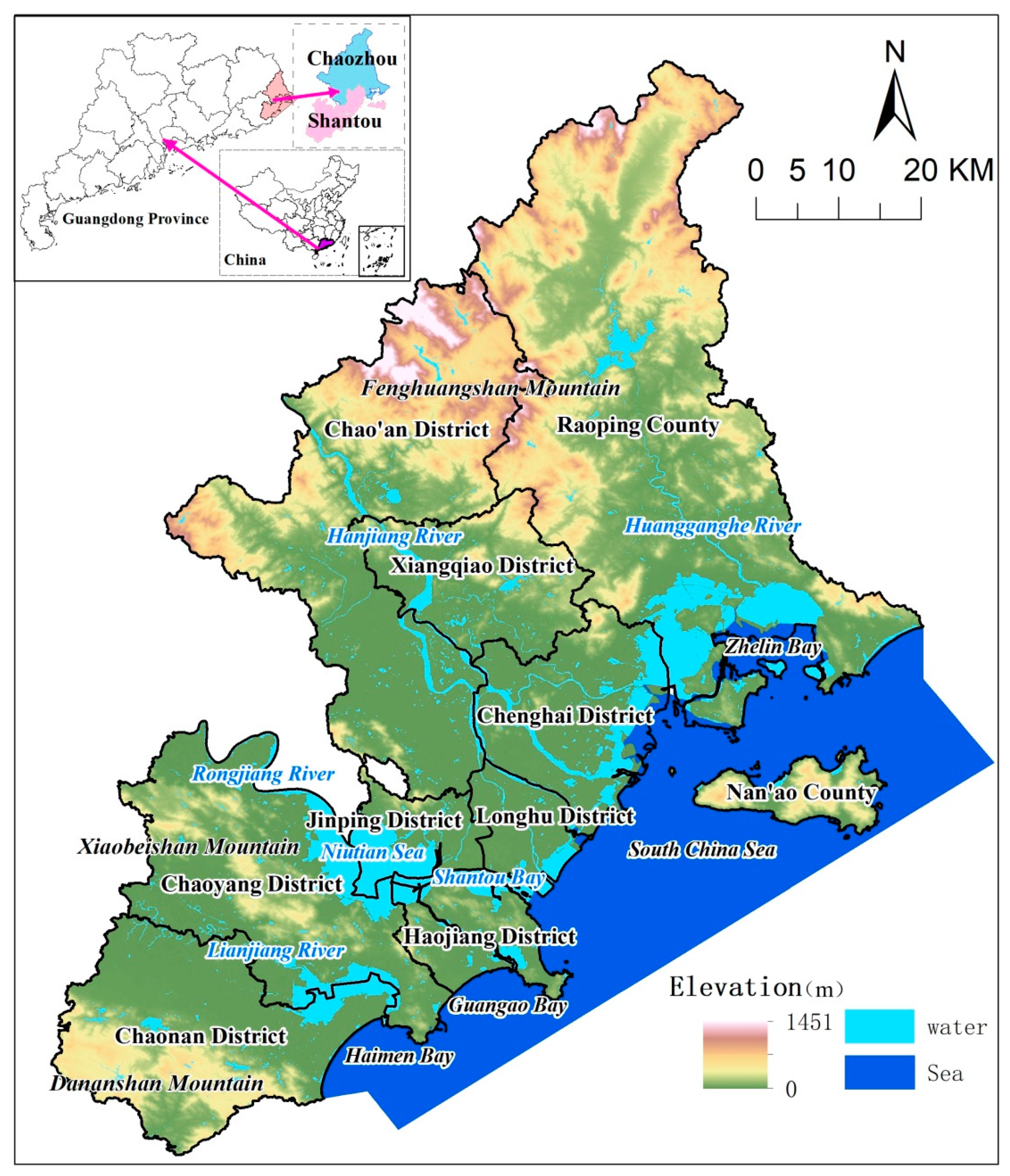
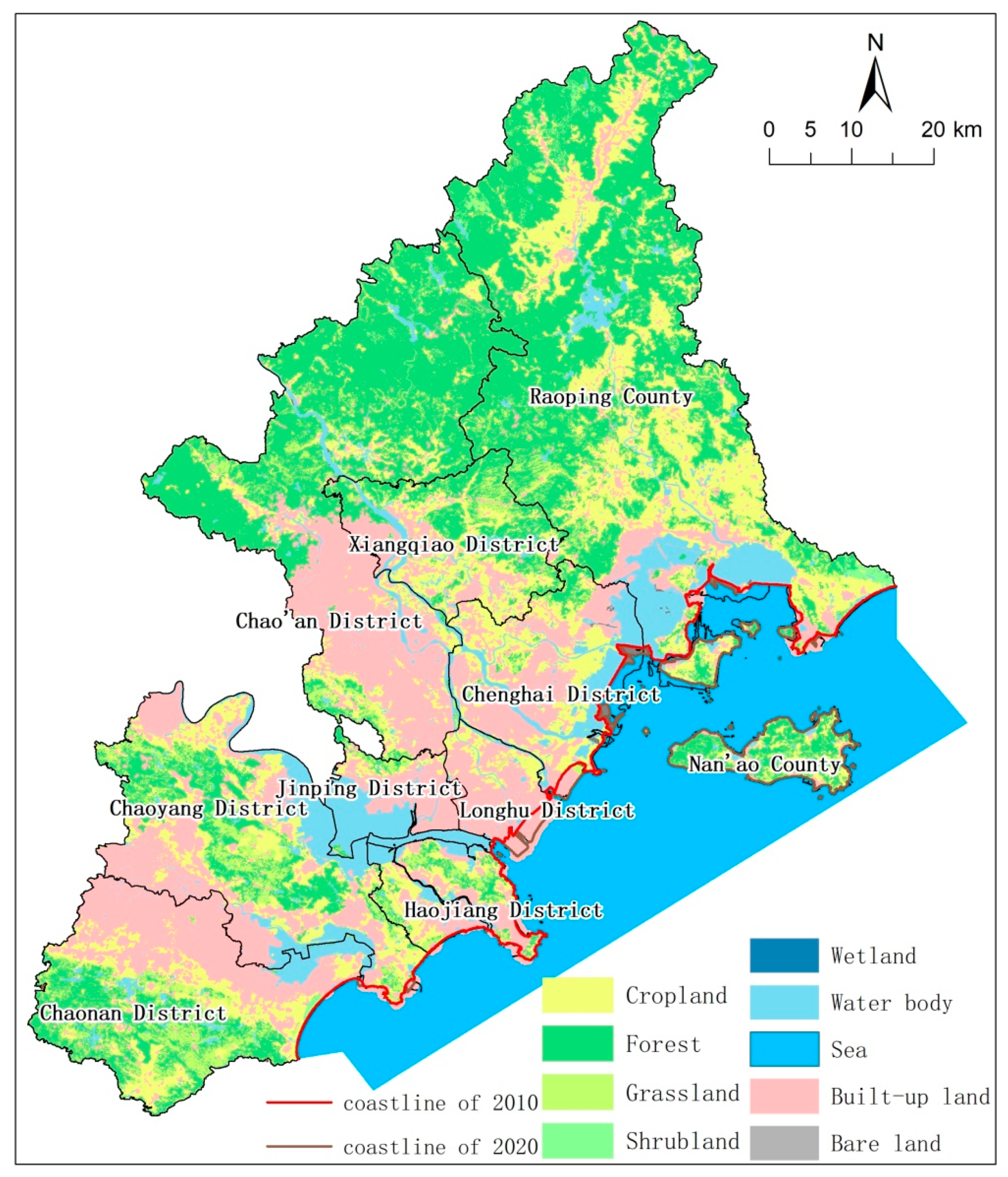
Chaozhou and Shantou are located in the east of the Guangdong Province (23°21′ N–24°14′ N, 116°14′ E–117°16′ E), where the coastline is facing the South China Sea (Figure 1). This region encompasses the unique, local Chao-Shan culture; people in this region share a similar lifestyle, the same cuisine, and the same Chao-Shan dialect. The total combined area of these two cities is 6632 km2 (including the sea territory), with a population of 8.32 million. Chaozhou is in the northeast of the EGD, while Shantou lays in the southwest. Chaozhou has three administrative regions at the county-level: Raoping County, Chao’an, and Xiangqiao Districts, while Shantou city has seven county-level regions, which are the districts of Jinping, Longhu, Haojiang, Chenghai, Chaoyang, Chaonan, and Nan’ao County. Even though the EGD is one of the most populous regions of the Guangdong Province, and many counties and towns are considered to be peri-urban areas, when comparing GDPs with the Pearl River Delta, it is apparent that EGD is the lesser developed area [70,71].
The terrain of the montane north and northwest regions in EGD is >1000 m and slopes gently down towards the southeast. There are three important rivers in the EGD—the Huanggang, Hanjiang, and Lianjiang—and the croplands and primary settlements concentrate along the Huanggang River valley, Hanjiang River plain, and Liangjiang River valley.
2.2. Data Sources
The land-use land cover data for 2000, 2010, and 2020 were obtained from the GLOBELAND30 platform (http://www.globallandcover.com (28 September 2020)), at a 30 m resolution [72]. In the GLOBELAND30 platform, the classification system is as follows: cropland, forest, grassland, shrubland, wetland, water bodies, tundra (subclass are shrub tundra, grass tundra, wetland tundra and bare land tundra), artificial surfaces (built-up land), bare land, permanent snow and ice. The following classifications were found for EGD: cropland, forest, grassland, shrubland, wetland, waterbody, artificial surfaces (built-up land), bare land, and seawater. A 30 m digital elevation model (DEM) was acquired from the 91Weitu website (www.91weitu.com (25 September 2020)). Vectors of the EGD administrative region were drawn by the authors according to the regional maps of the Department of the Natural Resources of Guangdong Province’s website (http://nr.gd.gov.cn/gdlr_public/map/3/index.html (25 September 2020)).
Normalized difference vegetation index (NDVI) data were composed [73,74] using Landsat 8 data (the images downloaded from www.earthexplorer.usgs.gov (30 September 2020), image date: October 2019, images resolution: 30 m, path/row: 120/43 and 120/44, respectively, product level: L1T). The correlations were processed by the software ENVI 5.2, and the correlation parameters were obtained from the MTL file in the product [75,76].
Vectors of regional railways, roads, highways, town centers, and ecologically sensitive areas were obtained by the master city planning of Chaozhou and Shantou. Socioeconomic statistics were derived from provincial and municipal level data. All raster data were rescaled to 30 m.
2.3. Methods
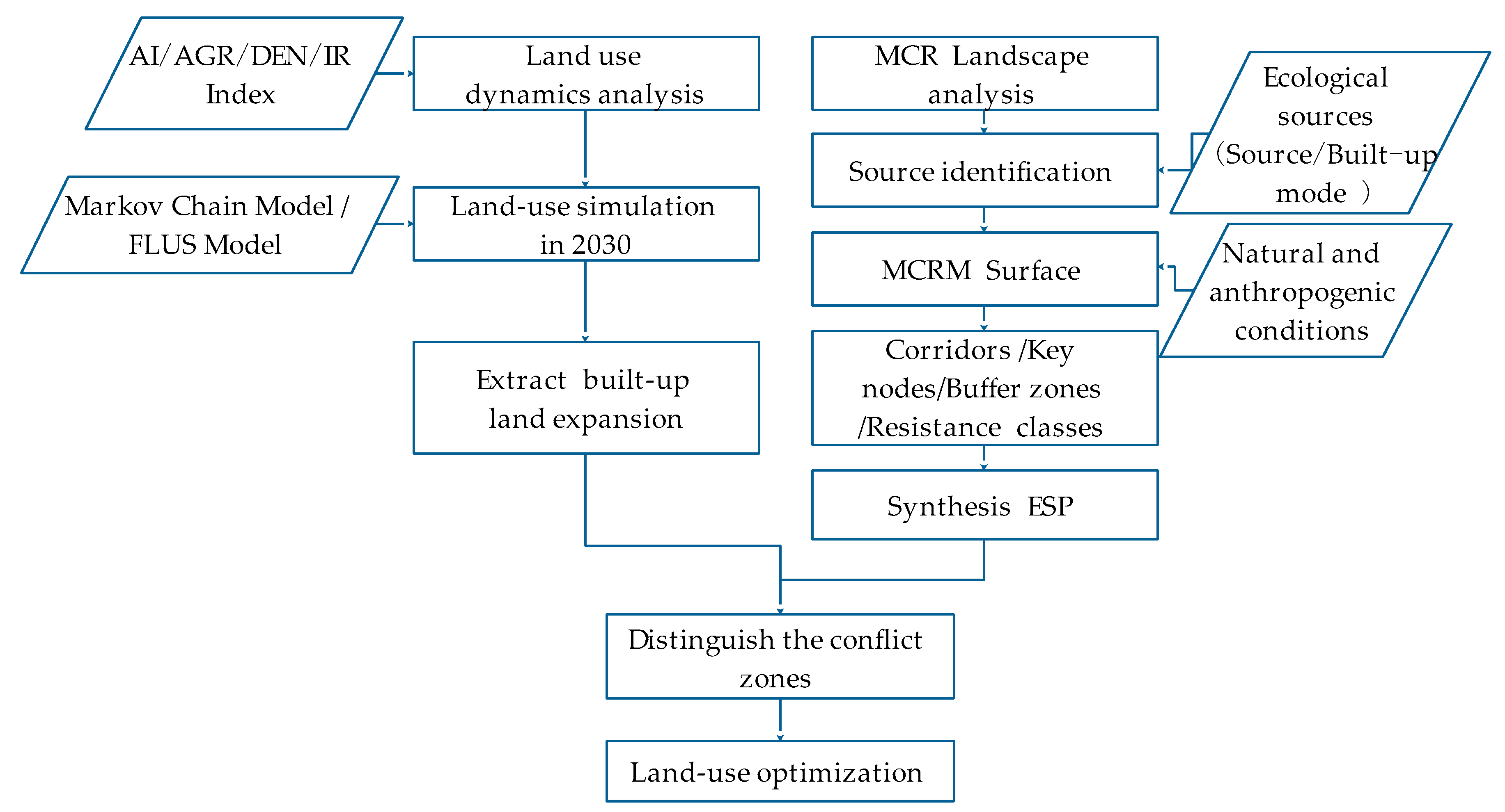
First, we used four indexes to analyze the land-use dynamics in EGD. Second, the methods of the land-use simulation process were demonstrated. The Markov chain model, which predicted the quantity of land-use types in 2030, was introduced. Then the detail of the FLUS model and the validation process were presented. Third, the concept and the process of establishing the MCR model were also presented. Finally, the ESP can be synthesized.
The schematic methodology is shown in Figure 2.
2.3.1. Land Use Dynamics Analysis
With the characteristic of land-use change [42], two indices, the annual increase (AI, km2·y−1, Equation (1)), and annual growth rate of croplands and built-up land (AGR, %, Equation (2)) were introduced to reveal the dynamics of these four typical and signature land-use types of EGD [77,78,79,80]:
where and are the areas of crop- (built-up) land at the initial and end times, respectively, and d is the analysis period in years (one decade). DEN stands for the proportion of built-up land in the study area. In Equation (3), denotes an artificial surface area, and A denoted the total area. The warning threshold for identification of “overdevelopment” according to international criteria are areas where DEN is >30%. Then we analyzed the increase in DEN increased rate (IR) where and are the DEN values in 2010 and 2020, respectively.
2.3.2. Markov Chain Model
To predict the quantity of each land-use type, a Markov chain model was introduced. Commonly used to predict geographical characteristics lacking after-effect events [81,82,83], this model has become an important prediction method in geographical research [84]. In this study, the Markov chain model calculated the probability matrix of land conversion and then analyzed the mutual transformation relationship of the different land-use types. By using a module integrated within FLUS software, the total amount of future land-use types in 2030 were predicted with a decade-long step of the transformation matrix.
2.3.3. FLUS Model
The FLUS model is software that combines the “top to bottom” system dynamics (SD) model and “bottom to top” CA model [36] and provided a multiple CA allocation model for simulating land-use change and scenario analysis. The “top to bottom” represents macroscale demands, such as political planning and background climate influences, while the “bottom to top” determines the system’s evolution from a local perspective [36]. By considering various socioeconomic and natural environmental factors, the SD model was used to project the land-use scenario demands, while the CA model processed complex interactions among the different land-use types [36,37]. FLUS has shown to have a higher simulation accuracy than the CA and CLUE-S models [36]. The model and further information can be found online (http://www.geosimulation.cn/flus.html (28 October 2020)).
In this study, nine classes of land-use were used (Section 2.2), and for an ANN-based suitability probability estimation module, a random sampling of 1‰ of the land-use raster was selected with 10 hidden layers. The driving factors included environmental and socioeconomic factors: DEM, NDVI, ecologically sensitive areas, town centers, railways, and main roads. Moreover, the factors were trained by the model and land-use data to obtain a probability distribution map. Then self-adaptive inertia and competition mechanism CA module were used to simulate the land-use change in 2030 based on the starting year of 2020.
Simulation results were validated using both Cohen’s Kappa coefficient and figures of merit (FoM) provided in the FLUS model. Some studies have shown that FoM is superior to the Kappa coefficient in assessing the accuracy of simulated changes [85,86,87]. The FoM is the ratio of the intersection of the observed change and predicted change to the union of the observed change and predicted change [86,88]. Equation (5) of FoM is as follows:
where B is the area of correct due to observed change predicted as change, A is the area of error from observed change predicted as persistence, C is the area of error from predicted change to an incorrect category, and D is the area of error from observed persistence predicted as change. Our study focused on the validation by the FoM method, while the kappa coefficient was still demonstrated for references.
2.3.4. MCR Landscape Analysis
In MCR landscape analysis, we used three steps: defining the ecological source, building the ecological resistance surface and identifying key ecological corridors. In the second step, the ecological resistance surface was established according to the MCRM.
Source Identification
Ecological source originally identified the habitat that species most relied upon [48,89], and recently this definition has been expanded to include those patches, which plays a crucial role in overall ecosystem health and are important for urban/regional ecological security [49]. In the present study, sources represent the main core areas for a particular ecological or artificial process. Two kinds of processes were acknowledged: natural or ecological processes and the expansion of human activity, categorized into the ecological sources (sources mode) and built-up modes, respectively. Ecological sources were obtained from the Chaozhou and Shantou master planning data, which identified the ecologically important and sensitive regions. Ecological sources included: forests of protected regions, protected drinking water reservoirs, and some important habitats for certain species. For sources of the built-up mode, we chose the built-up land from the 2020 land-use map >10 hm2.
MCRM Surface
Resistance means the difficulty for the species or ecological flows the move or travel to other places [89,90]. In the MCRM, the space of the study area was considered as a surface with different resistance values, and the resistance values were calculated in different evaluation systems. The MCRM is a mainstream assessment method, and it was widely applied to landscape design, which aims to protect natural ecosystems within specific secure borders [47], biodiversity conservation, and urban planning [62,90,91].
The MCRM calculates the required cost of species’ moving from the source to the destination. It reflects the potential possibility and tendency of species’ movement [48]. The MCRM can also be used to simulate different ecological flows across different landscape surfaces by establishing a minimum cumulative resistance path [49,92,93].
In our study, the MCRM surface was evaluated, and the evaluation contained two primary factors: natural and anthropogenic conditions. The natural factors included: DEM, NDVI, land-use types, geological hazards, risk (i.e., landslide or debris flow) and distance from water (rivers, ponds, reservoirs). Anthropogenic influences included: distance from built-up land, distance from roads (main city roads and highways). Elevation and NDVI data were standardized as the following equation [94]:
where represents the standardized value, x represents the original pixel value, max and min represent the maximum and minimum pixel value, respectively.
Geological hazard data were obtained from Chaozhou and Shantou geological planning, which defined risk into four levels: comparatively safe, low, medium, and high-risk. Using previous studies [48,49,91,94,95] and the conditions of the EGD, all factors were assigned scores from 0 to 100, where a higher score indicates a higher resistance. The weight of each factor was calculated using the analytic hierarchy process (AHP) method.
The equation of the MCRM is as follows (Equation (7)):
where f represents the relative function to the minimal resistance; represents the spatial distance of a target unit from the source point j to the land-use type i; and represents the ecological resistance of the spatial unit i to a target’s migration.
The MCRM contains two parts described as follows (Equation (8)) [94]:
where the MCR represents the total MCR, represents the MCRM based on the ecological sources, and represents the MCRM based on the built-up land expansion. and represent the difficulty for the land-use type to expand or develop from the center of the source to the surrounding areas. The higher the MCR, the more difficult the expansion, and details of the factors and scores with the weight can be seen in Table 1.
Determining Ecological Corridors, Key Nodes, Buffer Zones, and Conflict Zones
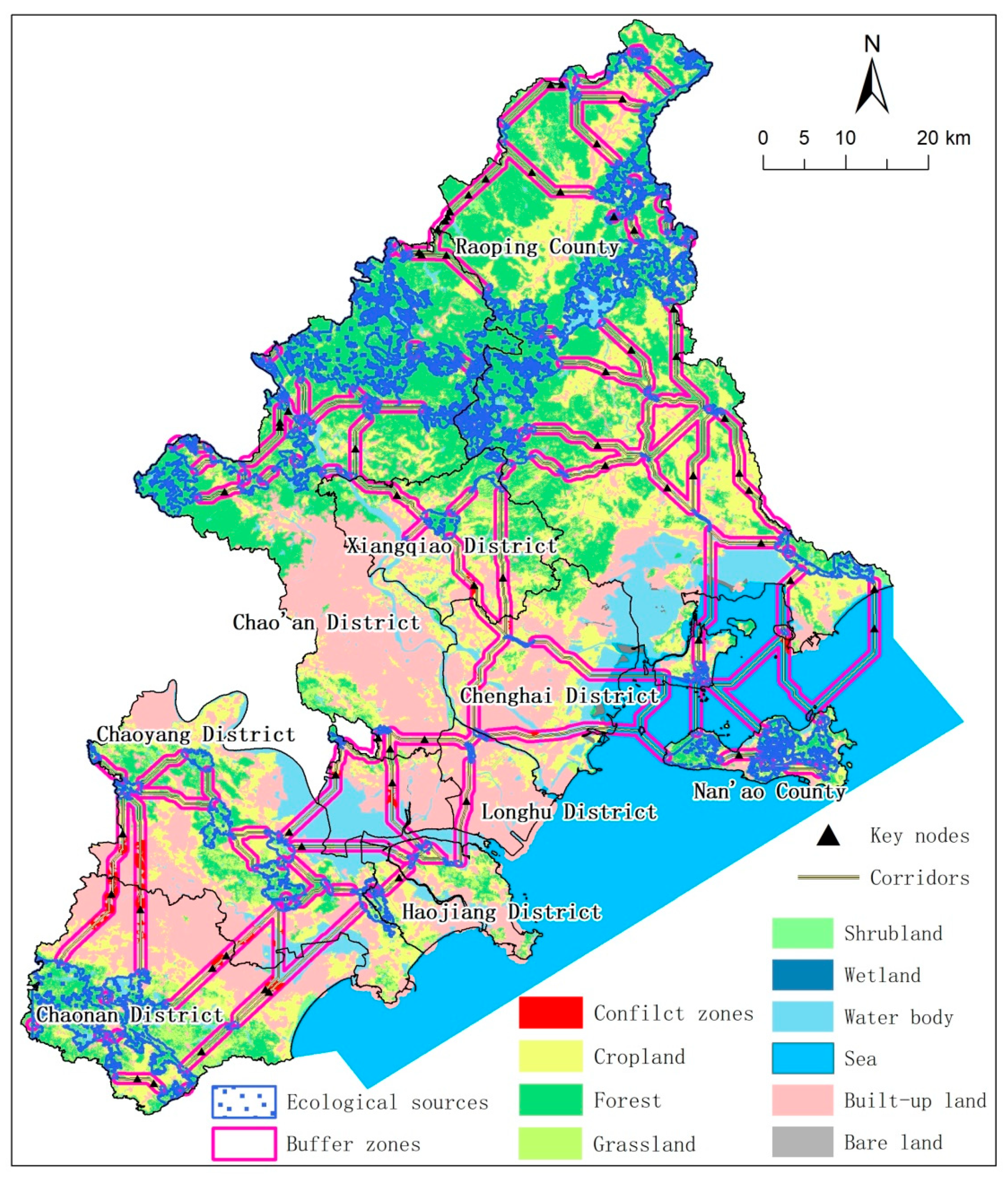
After identifying the ecological sources and setting up the resistance surface, it was necessary to connect them based on the MCRM surface analysis. The least-cost path method was applied to establish the corridors, and the corridors connect the ecological sources. In our study, the least cost path was calculated by the tool of linkagemapper (https://circuitscape.org/linkagemapper/ (14 January 2021)) in ESRI ArcGIS (v.10.2), and the linkagemapper is a commonly used tool in ecological and habitat studies [96,97]. A 40 km threshold was used to truncate corridors between sources, with a maximum number of connected nearest neighbors set to four after tested. Key nodes, which represent the place that had equal resistance values between every two ecological sources, were considered to be crucial to the process of maintenance and migration of species [48]. Moreover, the key nodes were identified through the watershed method toolbox in ArcGIS. Buffer zones of 600 m were set up around the center of each corridor. Conflict zones are the most sensitive and fragile regions in need of future protection. We simulated the increase in built-up land for 2030 using the FLUS model and labeled the intersection of areas where new built-up land occurred and buffer zones as conflict zones. The conflict zones are the concern for future land-use management.
Synthesize the ESP
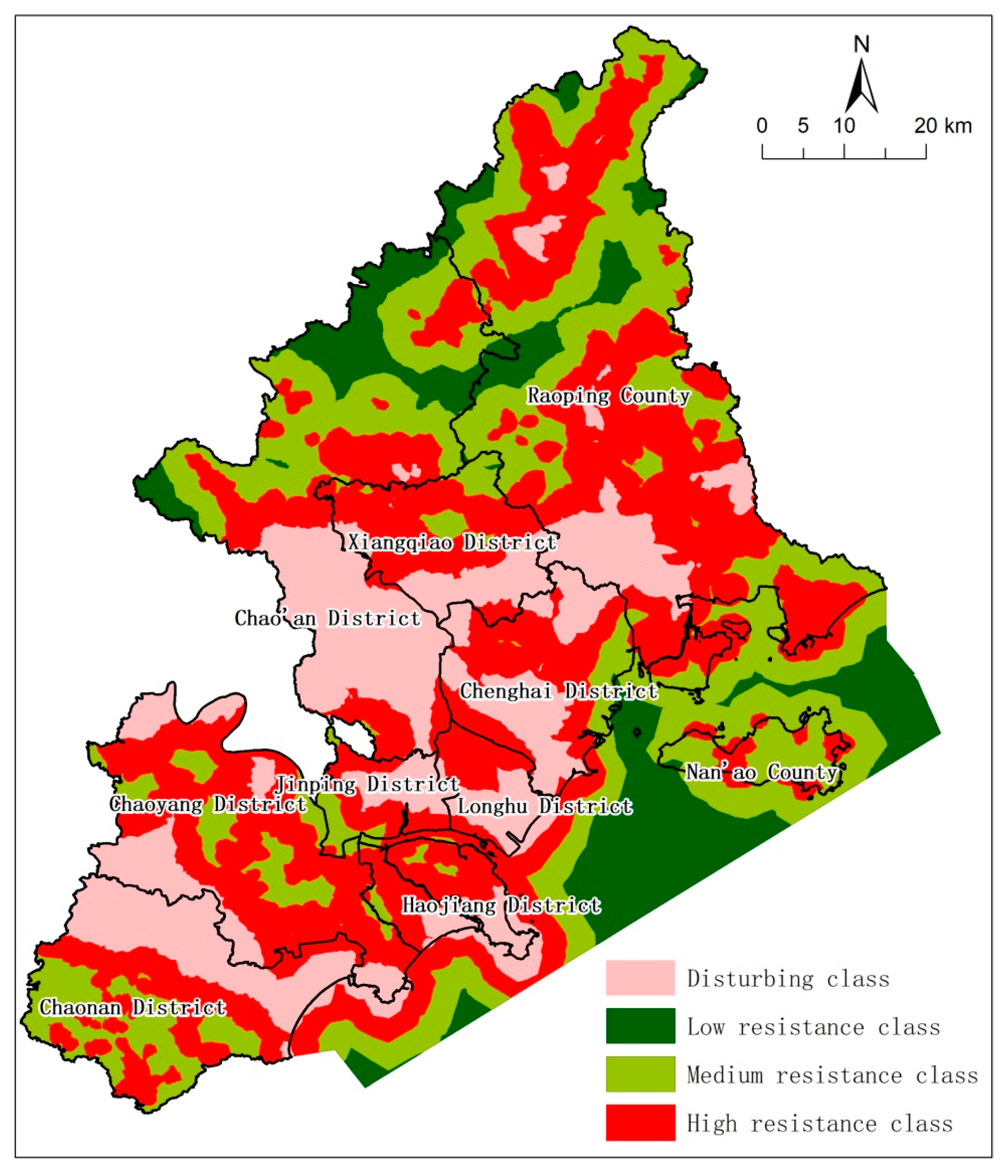
Apart from the built-up land (artificial surface) of 2020, the MCRM surface result was classified into four classes with natural breaks (Jenks) using ArcGIS, each representing the relative ecological importance: disturbed class, where the most frequent human activities occur; low resistance class, the most important areas, which may require protection any time; medium resistance class, average importance of the EGD; and high-resistance class, areas that need the least protection.
With the ecological sources, corridors, buffer zones, and key nodes ad the resistance classes, an ecological security pattern (ESP) was established. By analyzing the ESP, the corridors, key nodes and the spatial conflict between the land-use simulation results in 2030 of the FLUS model with these patterns, ecologically sensitive and fragile regions were identified, presenting the optimized land use.
3. Results
3.1. Land Use Dynamics in EGD
3.1.1. Spatial and Temporal Changes in EGD
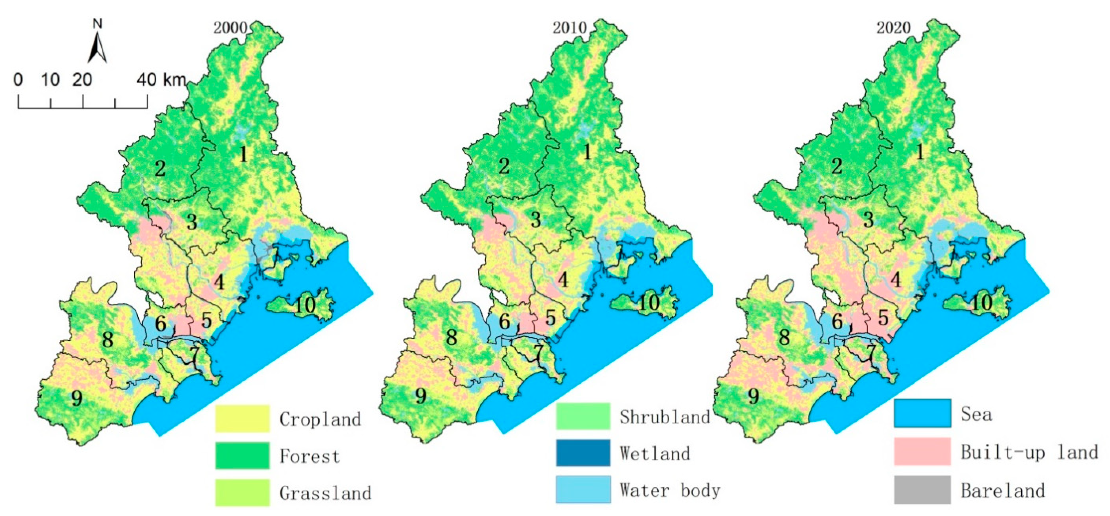
Table 2 shows the areas and proportion of land use for the three time periods. As shown in Figure 3, forests are the most distributed land-use type in EGD, located primarily in the north and southwest. Cropland is the second most distributed land-use type, mainly found in the north, east, central, and southeast of EGD.
Croplands and built-up land received the most attention from previous studies of EGD land-use [42,98]. Although the quantity increased, the proportion of cropland remained nearly the same in the first decade (Table 2). Cropland AI and AGR were 239.67 hm2·y−1 and 0.14%, respectively, from 2000 to 2010, while its quantity dropped down by ~5% from 2010 to 2020, where AI was −3856.44 hm2·y−1, and AGR was −2.52%. Built-up land was stable from 2000 to 2010, with an AI and AGR of −219.12 hm2·y−1 and −0.37%, respectively, but it increased from 8.67% to 15.31% from 2010 to 2020, with an AI and AGR of 4386.82 hm2·y−1 and 5.85%, respectively (Table 3). Since EGD is located along the South China Sea, the study here also focused on the coastline and the sea. Seawater area dropped to 19.75%, indicating that EGD acquired land from the sea during 2010–2020 (Table 2).
3.1.2. Land Use Transition Matrix Analyses
In the first analysis period (2000–2010), the most significant transformation was from built-up land to cropland, accounting for 5400 hm2 (Table 4). The transformation from cropland to a water body (4821 hm2), and the reverse (4360 hm2), were also high. The amount of area converted from grassland to forest was also nearly equal to the opposite conversion.
Table 5 shows the transformation areas from 2010 to 2020, where the strongest pattern was cropland becoming built-up land (36,050 hm2). Croplands were also being encroached upon by water bodies (>4500 hm2). Over the same period, the sea area was also diminished by built-up land, at a scale of 1242 hm2.
Table 2, Table 3, Table 4 and Table 5 show that during the two decades of analysis, croplands in EGD decreased from built-up land expansion and conversion to water bodies, where the latter can be explained by local farmers changing focus from traditional agriculture to aquaculture. Built-up land gains were derived primarily from croplands, and the sea and total conversion into built-up land took up a large proportion of all the land-use transformations. The tradeoff between cropland and built-up land was the most significant problem of the EGD over the past two decades, and it will likely continue to be a central priority of territorial planning for the future.
3.1.3. Land Use Change Characteristic Analysis
Two typical land-use types—built-up land and cropland—were chosen to analyze their changing spatial characteristics.
Over the previous two decades, transitioning into built-up land was the most significant land-use change of the EGD. From 2000 to 2010, built-up land expansion was scattered throughout EGD, and the relatively small-scale expansions were located in the central and southern Chao’an District, south of the Chenghai District, along the Lianjiang River valley in the southeast of EGD, and road construction in the south of Raoping County. In the second decade of analysis, built-up land expansion was at a significantly larger scale and distributed more broadly. The largest expansion during this period was located along the sea, in a reclamation area from Shantou. The south and middle of Chao’an County, the north and west of Chenghai District, and expansion along the Lianjiang River valley were also quite high.
The amount of cropland decreased during these two decades. From 2000 to 2010, the decrease in cropland was relatively small and mainly occurred around the Chaoyang and south of Chao’an Districts. For the second period, the decrease in cropland was broadly located throughout the entire study area, and these spatial distributions were highly consistent with the expansion of built-up land in the south and central Chao’an District, west and south of the Chenghai District, the center of Shantou, and along the Lianjiang valley. In the southwest of Raoping County, the decrease in cropland derived from conversion into water boded for the aquaculture.
3.1.4. Development Intensity
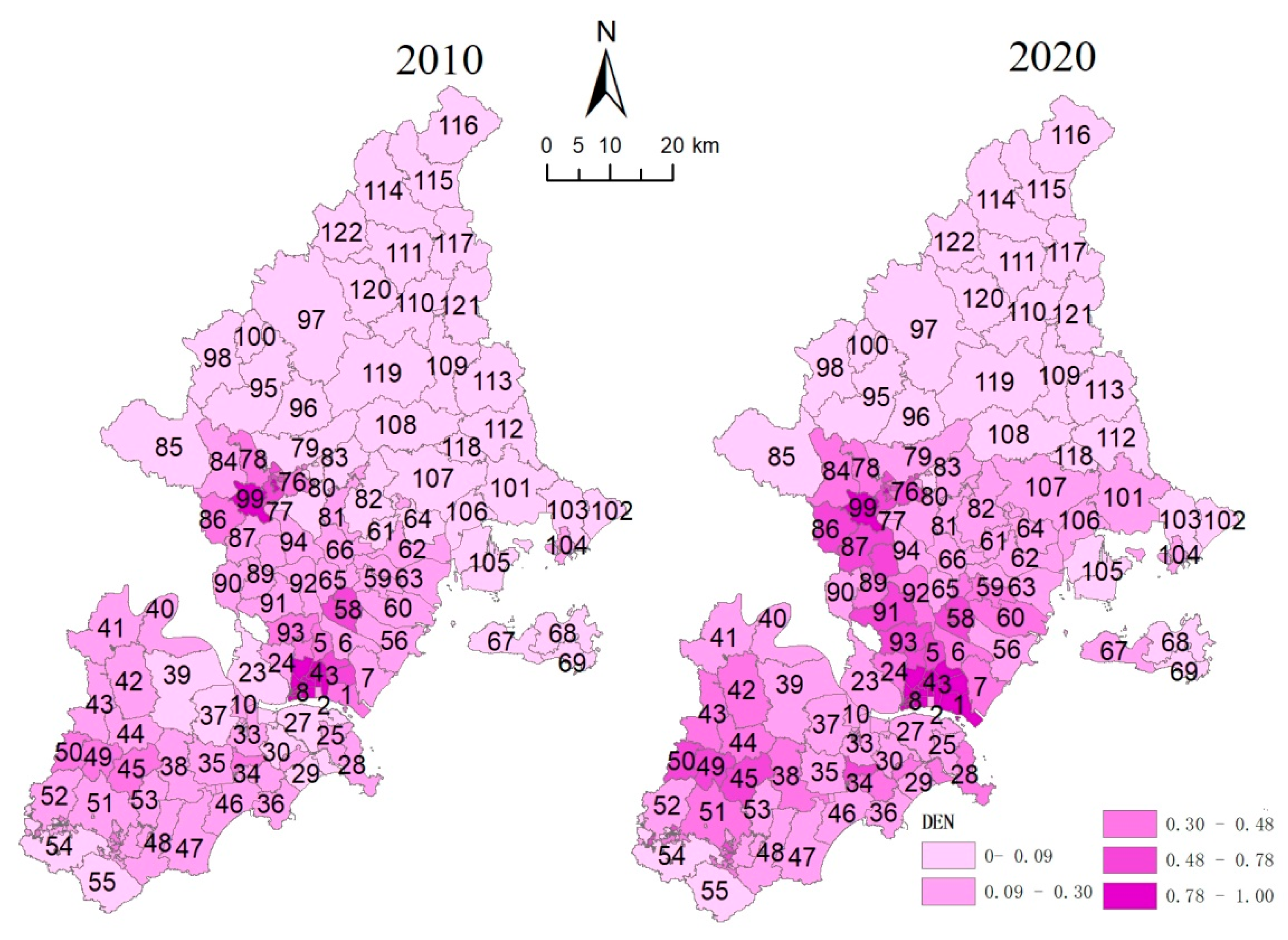
It was found that built-up land expanded significantly from 2010 to 2020. According to E (3), the DEN of the entire EGD in 2010 and 2020 were 10.73% and 18.92%, respectively. The DEN of all county levels was from 2.15% to 33.19% in 2010, with the highest intensities occurring mainly in the center of Shantou, particularly in the Longhu and Jinping Districts (Table 6). At the same time, the Chaoyang and Chaonan Districts were also in a relatively high-intensity location. In 2020, it was apparent that the DEN increased at a rapid pace, where Longhu and Jinping Districts still maintained the largest two DEN values, and five other district/counties were also >20%. Haojiang District and Nan’ao County increased by >200%, indicating that these two administrative regions developed at a significant pace.
DEN at the township-level was also analyzed (Figure 4). In 2010, 37 of the 122 towns in EGD exceeded 30%. These towns are mainly distributed in the center of Shantou, south of the Chenghai District, the center of Chao’an District, and north of Chao’an District. In 2020, 57 of the 122 towns exceeded the international criteria, distributed from the central Chao’an District to the southeast of Shantou and along the Lianjiang River valley. Meanwhile, there were 16 additional towns > 20%, together indicating that the built-up land expansion was intensive over the previous decade. Table 6 demonstrates the DEN of each district/county in 2000 to 2010 and 2010 to 2020 periods.
3.2. Land Use Prediction and Simulation Results
Based on the land-use data of 2000 and 2010, a Markov chain prediction module in the FLUS software was used to predict land use in 2030. For validation, the kappa coefficient and FoM were calculated as 0.86 and 0.35, respectively, which were the precision validation parameters of 2020 [35,36,87]. The parameters indicated that 2030 predictions were reliable, and the simulation results can be seen in Table 7.
The simulated results shown in Figure 5 indicated that the expansion of built-up land continued to take over cropland s of the EGD, particularly in the Lianjiang River valley, south and central Chao’an District, south Raoping County, and east of Shantou, all of which are presently occupied by tremendous croplands. Furthermore, the built-up land encroached upon the sea for all districts and counties along the South China Sea. Far fewer land-use changed were predicted in the north and central EGD.
3.3. MCRM Results and Ecological Security Pattern (ESP) Establishment
3.3.1. Source Distribution and MCRM Results
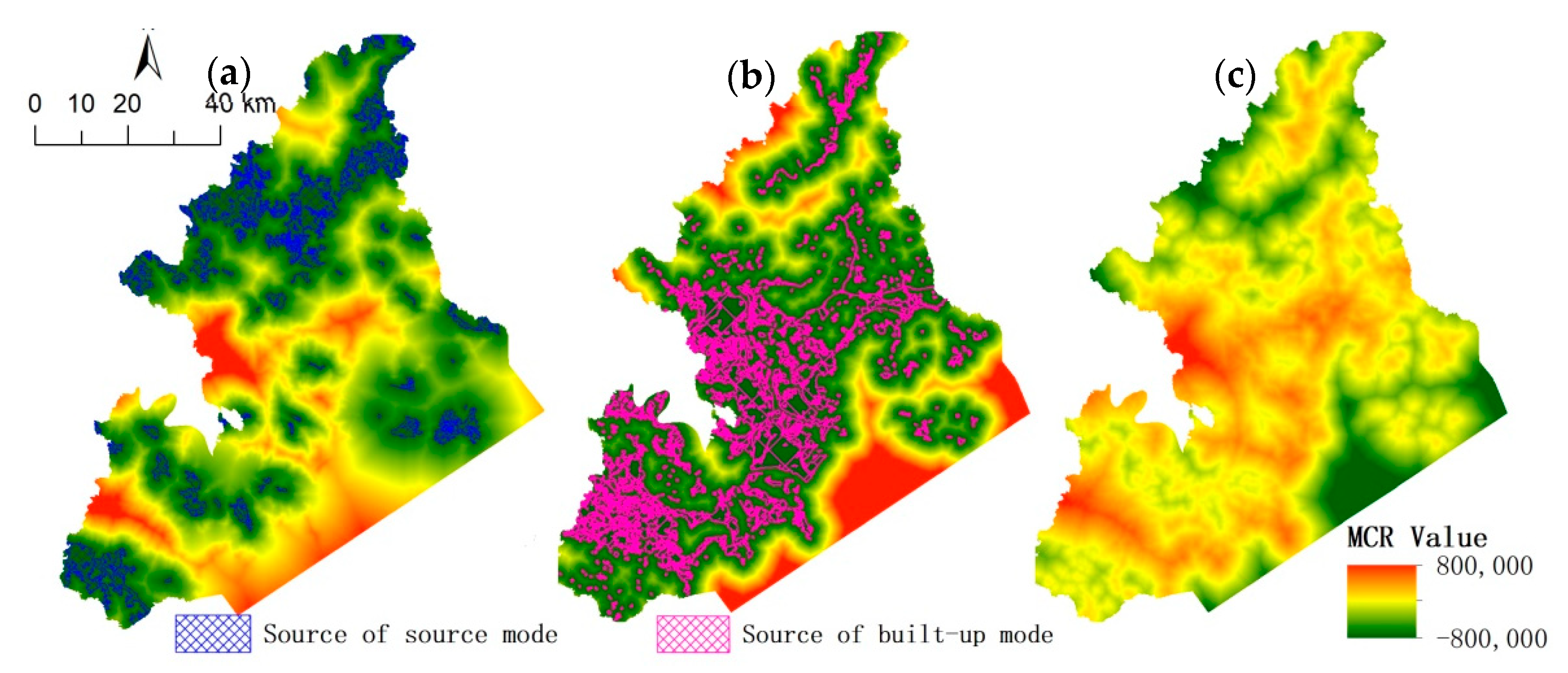
As mentioned above, the ecological sources were obtained from the Chaozhou and Shantou city master plans. According to the land-use types, the primary ecological sources were forests and water bodies (i.e., rivers and reservoirs) scattered throughout EGD. Spatially, both were concentrated in the north and southeast, such as the northern Chao’an District, northern and central Raoping County, southern Chaonan District, central Chaoyang District, and two-thirds of Nan’ao County. These resources are currently protected by law and cannot be destroyed or encroached upon by any authorities or persons. Built-up mode sources were readily recognized in Figure 6, showing the MCRM calculation results of the two modes.
The disturbing layer accounted for ~21.13% of the total study area (1401.34 km2), located mainly around the Lianjiang River valley, the center of Shantou, southern and central Chao’an and Xiangqiao Districts, and a belt along the coastal sea (Figure 7). The low class accounted for ~10.67% of the study area (707.63 km2) and was mainly concentrated in the north and southwest, corresponding to the montane and pelagic regions of EGD. The medium class proportion was 28.82% (1911.34 km2), and located adjacent to the low class south of Chaonan District, central Chaoyang and Chao’an Districts, and northern Raoping County. The high class accounted for the greatest proportion of the EGD, 39.37% (2611.02 km2), and surrounded the disturbing layer. This phenomenon showed that the high class had a strong correlation with human activities, and any further expansion of built-up land would encroach the high-resistance areas first.
3.3.2. Ecological Corridors, Key Nodes, and Buffer Zones
One hundred seventeen corridors were established by the linkagemapper based on the MCRM surface analysis, and the lengths of the corridors were between 30 and 22,245 m (Figure 8). The mountainous regions of the north, the southeast, and the southwest were concentrated with a greater number of corridors, which were also more curved than in the plain regions; whereas the plains, like the center of Raoping County, the south and center of Chao’an District, and the center of Shantou, maintained fewer corridors with a more direct morphology. The key nodes were mainly distributed in the middle and the north of Raoping County, the border between Chao’an District and Raoping County, north of Chao’an District, the center of Shantou, the south of Chaonan District and the Lianjiang River valley. Using the corridors as the center, 600 m buffer zones were also created and can be seen in Figure 8.
3.4. Optimization of Future Land Use
3.4.1. Conflict and Fragile Zone Identification
After obtaining the buffer zones, we analyzed the spatial relationship between the ESPs and the buffer zones and found that the low-resilience, medium resilience, high-resistance and disturbing classes accounted for 6.16%, 35.20%, 48.22%, and 10.42%, respectively. The buffer zones in conflict with the low-class ESPs were mainly distributed in the north of Raoping County and connected to Na’nao County. The medium class conflict zones were mainly located in the north of Chao’an District, the northeast of Raoping County, the areas between Raoping and Na’nao Counties, and the middle of Chaoyang District.
To optimize future ecological land use, it is important to identify conflicts between the buffer zones and human interface; to this end, we extracted the increase in built-up land from 2020 to 2030 based on the simulated results of the FLUS model and analyzed the spatial fragility and conflict areas. The buffer zones with increasing built-up land were mainly distributed in the areas around the Lianjiang River valley in the Chaoyang and Chaonan Districts (Figure 9). The statistics indicated that the Chaoyang-Chaonan areas represented > 80% of the conflict zones in the whole study area (35.32% and 45.21%, respectively). For the remainder of the conflict zones, the Jinping, Xiangqiao, and Chenghai Districts maintained > 8.61%, 5.38%, and 3.75%, respectively. The Longhu District and Raoping County maintained 1.53% of the conflict zones of the whole study area. 89.97% of the increased built-up land were within the disturbed ESP zones, while 9.04% and 0.99% were within the high and medium ESP classes, respectively.
3.4.2. Land Use Optimization in EGD
Conflict and fragile zones of the corridors, as well as built-up land (including 2020 measurements and 2030 simulated results), which encroached upon the low class of the ESP, should be reclaimed or remain in their original land-use type to best preserve ecological resources. There were 24.4 hm2 of built-up land in the low class observed in 2020 scattered in the northern Chao’an District and central Raoping County. There were 369.70 hm2 and 94.32 hm2 of built-up land in the medium class of 2020 and 2030, respectively. The transitional nature of the medium class implies that they are also important to protect. Thus, the areas mentioned above should be the focus of land conservation plans in all future efforts.
The simulated results showed built-up land expansion into the water along the coastal South China Sea (Figure 8), with the greatest changes located on coastlines of Chaoyang, Haojiang, Longhu Districts, and Raoping County; however, in 2015, the MNR enacted a policy to ban reclamation from the sea to protect the pelagic and coastal ecology. Thus, the simulated results are not plausible, and all planned reclamation of the sea in the predicted territorial planning can be ignored if the present conditions are upheld.
We also analyzed the spatial relationship between the ecological sources and the built-up land. No simulated built-up land was found to occupy the ecological sources in 2030, while 129.01 hm2 were recorded in 2020. Although the patch scales were relatively small (average area, 1.6 hm2), they were scattered nearly throughout the entire study area: 44.83% located in the Chaonan District, primarily in the south and montane regions; 15.66% in Chaoyang District, which were also confined to the mountains; patches of the Chao’an District, Nan’ao, Raoping Counties, and Haojiang District were also in the mountainous areas, with proportions of 10.17%, 7.38%, 6.69%, and 4.81%, respectively; and in Chenghai and Longhu Districts, the patches occupied the protected drinking water reservoirs, comprising 3.16% and 5.19% of all patches observed. The results indicated that all of these patched areas should be reclaimed to their non-artificial surface conditions in future territorial plans to best preserve the region’s ecological resources (Figure 8).
4. Discussion
4.1. EGD Built-Up Land Expansion and Management
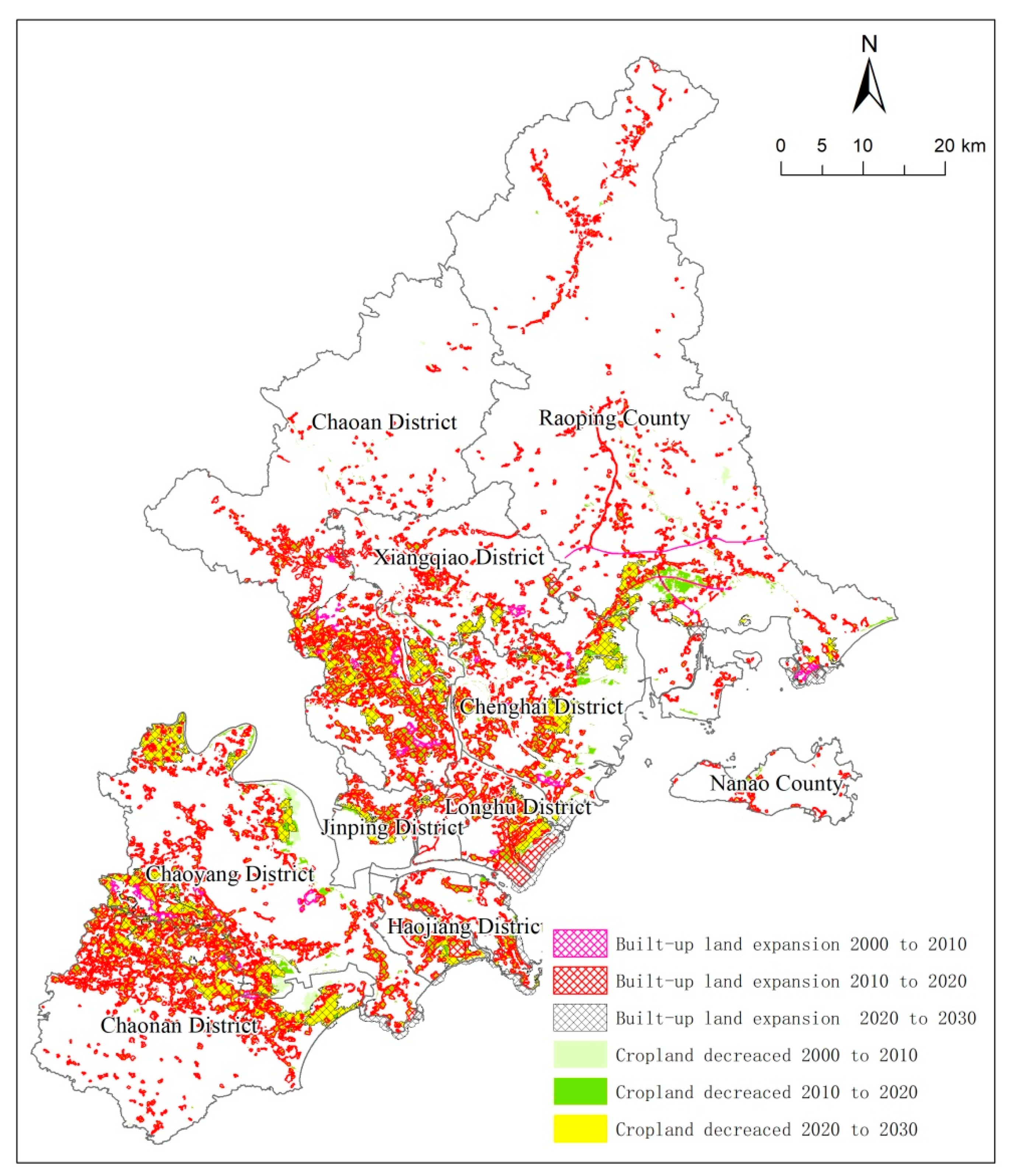
As shown in the previous section and from Figure 9, many areas in EGD underwent intensive built-up land expansion over the past decade. Many towns exceeded development intensity by 30%, some located in the city centers, but many others in rural areas. For example, some of the towns in Chao’an and Chaonan Districts were close to exceeding 60% development. By combining the development intensity of built-up land and the land-use map of EGD, we revealed three hotspots of built-up land: (1) the spread and sprawl belt of built-up land from the middle of the Chao’an District to the southeast towards Shantou’s city center; (2) the intensive development along the Lianjiang River valley, located north of Chaonan and Chaoyang Districts, starting from the west of the Chaonan District and spreading east to the South China Sea coastline; and (3) starting from the south of Shantou Bay, and traveling along the coastline until reaching the northeast of Raoping County. These vibrant belts are the focus of EGD’s manufacturing industry, most of which belong to small businesses or private companies. The primary industry of Chaozhou City and the surrounding suburbs is pottery. The south of Chao’an District, to the west of Shantou, is dominated by food industries, package printing, and machine manufacturing. The north of Shantou, like the Chenghai District, is a center of toy manufacture and assembly. To the south of Shantou, such as the Chaonan and Chaoyang Districts, the main industries are textiles and printing.
After analyzing the development intensity of the EGD over the past decade, we concluded that built-up land expansion was mainly concentrated in the suburban areas around the cities of Shantou and Chaozhou (Figure 9). It is widely acknowledged that the greater the intensity of built-up land expansion, the greater the correlated ecological and social problems [10,99,100]. Empirical studies have indicated that the scale of built-up land in these areas should be constrained [52,53,101,102] and restored to natural land cover types whenever possible for a more sustainable level of development.
The rapid expansion of built-up land allowed the economy to thrive in these areas over the past decade; however, it came at the sacrifice of the cropland area, as revealed by the land-use transition matrix. These plains areas made a significant contribution to the local agricultural industry and essential to China’s policy of protecting croplands, especially those of high productivity. Thus, it is essential to prevent the further spread of built-up land encroaching on the high-quality croplands of the EGD.
Built-up lands also encroached upon on the South China Sea, and during 2010–2020, the conversion from sea to built-up land was > 1242 hm2, with an additional > 800 hm2 of grassland converted from the sea as well. According to the master city plans of Chaozhou and Shantou, conversion from the sea was one of the major paths to increase built-up land. The conversion of the sea in Shantou occurred in three areas: Chaoyang-Chaonan, Haojiang, and the Longhu-Chenghai. For Chaozhou, sea conversion occurred exclusively in Raoping County. Reclamation in Chaoyang-Chaonan and Raoping County was mainly for the manufacturing industry, whereas conversion in Longhu, Haojiang, and Chenghai were for the construction of the new Shantou city center.
Studies showed that the sea reclamation had a negative impact on the coastline. First, it slows down the flow of the sea, and the self-purification capability of the sea would also go down. Second, the sea reclamation destroys the natural coastline, and it lowers the capability facing the tides and storm [103]. Historical, Shantou City lost over 500 hm2 from 1950s to 1980s due to the sea reclamation, and it affected the biodiversity around the coast [104,105]. All planned reclamation projects from the sea before 2020 were carried out; however, the simulated results from 2030 showed that sea reclamation was still a hotspot for the increase of built-up land, despite the Chinese federal government, the MNR, and the Guangdong provincial government announced that reclamation from the sea is prohibited except in special circumstances. Moving forward, it will be nearly impossible for the EGD to reclaim any further area from the sea.
New policies regarding the renewal of old and low-efficiency neighborhoods will be necessary for future, sustainable spatial planning. It is recommended that the governments conduct full investigations to find these low-efficiency, dated, and built-up areas, which lack necessary facilities and are in need of increased residences. The specific policy for renewal and land consolidation should be formulated so as to meet the needs of the local residential demand. Old and inefficient areas usually are located within the city center, county, or towns, such as the southwest center of Shantou, south of Chao’an District, the center of Chaozhou, and the south of Raoping County.
4.2. EPS Optimization and Ecological Conservation
Environmental problems, such as water, soil, and air pollution, have had negative impacts on the EGD due to unsustainable developmental practices [106,107,108,109], and some of their negative impacts may be irreversible. In the background of the New Era, ecological civilization, and rapid expansion of the built-up land in EGD, it is crucial to protect the environment and preserve the ecological resources. The ESP, which was established according to the MCRM, demonstrated the spatial distribution of different ecological security levels. It provides basic regional protection for the necessary ecological areas and also guides the future built-up land expansion. The spatial management rules and the optimization in the study area should be categorized according to the resistance classes and the elements of the ESP (i.e., the corridors, the buffer zones or the areas around them).
The MCRM, which combined the natural conditions and anthropogenic factors, showed that the highest resistance areas are focused on the cluster of built-up lands. After establishing the ESP of the region, the low and medium resistance classes were identified that require prioritized protection and preservation. Low resistance areas, such as the north and middle of Chao’an District and Raoping County, the coastline around Na’nao County should be prioritized. This will present certain challenges based on the disturbances caused by human activities. We suggest that these areas should be strictly protected from any future land-use change or disturbance, and regulations should be set up to protect these areas. The present built-up land in the low resistance areas and the conflict zones should be identified in the consolidation plan. The medium resistance areas, especially the mountainous areas in Chaoyang District and Chaonan District, and the middle of Chao’an District should also be monitored by the local government. In addition, construction or potentially harmful activities should be constrained, as the preservation of these areas with low-resistance is vital. Negative impacts on high-resistance areas should also be regulated, although less strictly. Due to the critical importance of the corridors and buffer zones, they should be treated as low-resistance areas of the ESP.
The corridors play an important role in maintaining the landscape. In our study, the buffer zones were also identified. These two elements improve landscape connectivity, and landscape connectivity is a key factor in protecting regional ecosystem stability [110].
Conflict zones should be restricted from conversion to built-up land, thus preserving their original land-use type. This optimization can prevent anthropogenic interference and maintain landscape connectivity to promote ecological management. Local governments should strictly monitor and enforce any illegal encroachment into these areas because these areas are hotspots for built-up land expansion, and the likelihood of encroachment is greatest in these areas.
We should emphasize that the low-resistance class of the ESP, corridors, and the conflict zones should be considered as the ecological baselines in territorial planning. This does not mean, however, that these should be the only areas that are protected. All future built-up land expansion should be considered carefully to avoid negative ecological effects.
The built-up and low-resistance lands in 2020 should be categorized into the land consolidation and spatial territorial plans. Initially, the local governments should conduct ownership investigations and establish the ownership timeline of these areas, to distinguish any illegal claims under the current laws. Then, all applicable areas should be reclaimed to their pre-built-up status to preserve the ecological importance while fining the owners for illegal operations and encouraging the legal owners to move to less ecologically sensitive areas. Finally, the governments can also install specific reclamation plans according to the specific characteristics of these areas.
4.3. Study Limitations and Future Prospects
Our study used the MCRM to classify the ESP, combining natural and socioeconomic factors. Although we had eight factors included in the MCRM, due to the limitation of the data, additional environmental parameters, such as pollution and meteorological data, would likely increase the accuracy of the model.
The restricted area of the FLUS model provides users an option to restrict land-use changes in certain areas with additional spatial data input. In this study, the ecological resources were used as this restriction, implying they cannot be changed to other land-use types. Permanent basic farmlands are included in the cropland area, and they are relatively high-quality cropland. These croplands are protected by law and should not be encroached on under any circumstances. The permanent basic farmlands should also be considered as restricted areas in the FLUS model. If we can obtain this data, the simulation of cropland dynamics would be more accurate.
In this study, the quantity of built-up land in 2030 was predicted by the Markov chain model based on the land-use dynamics pattern in the past. However, the predicted result neglected other factors, such as the built-up land per person in the region, which was an important index in territorial spatial planning, the spatial unbalance of development and so on. In the future, further studies should focus on multiobjective decision prediction in the quantity of land-use types, which can be applied in spatial territorial planning.
5. Conclusions
Using the land-use land cover products from GlobeLand30, we analyzed the land-use dynamics of the EGD, including the cities of Chaozhou and Shantou, from 2000 to 2020. The conversion matrix showed that from 2000 to 2010, the quantity of cropland and built-up land was stable, whereas from 2010 to 2020, cropland dropped dramatically, and built-up land increased by 5.85%. The coastlines were also encroached upon by built-up land during the same period. We simulated land use in 2030 using a FLUS, and based on an MCRM, revealed the following distributions of ESPs in EGD: the disturbed class, 21.13%; low resistance class, 10.67%; middle-resistance class, 28.82%; and high-resistance class, 39.37%. The ecological resource locations were obtained from the master city plans for both urban areas, and a least-cost path to establishing the corridors and the buffer zones was proposed to improve landscape connectivity. By comparing the increased built-up land of 2030, the corridors, and the buffer zones, we have outlined an optimization plan by focusing on the hotspots for future built-up land expansion for the EGD; this can be applied in the spatial territorial planning. Additional measures and policies, such as preservation of the ecological sources, protection of cropland and coastlines, and consolidation of built-up land with low-resistance, were proposed for this and other similar areas in China with comparable development levels.
Supplementary Materials
The following are available online at https://0-www-mdpi-com.brum.beds.ac.uk/2071-1050/13/6/3473/s1, Table S1: the DEN and increased rate (IR) of EGD in townships.
Author Contributions
Conceptualization, Y.L.; methodology, Y.L.; formal analysis, G.H.; supervision, G.H. and S.C.; writing—original draft preparation, Y.L.; writing—review and editing, Y.L. and G.H.; visualization, S.L., W.L. and J.L.; software, S.L., W.L. and J.L. All authors have read and agreed to the published version of the manuscript.
Funding
This research was funded by the GDAS Project of Science and Technology Development of China, grant number 2019GDASYL-0105001; National Natural Science Foundation of China (4177012472).
Institutional Review Board Statement
Not applicable.
Informed Consent Statement
Not applicable.
Data Availability Statement
The data presented in this study are available in the supplementary material.
Acknowledgments
We would like to thank Xiaojun Feng (Guangzhou Institute of Geography, Guangdong Academy of Sciences (GGIG)), Yali Dai (GGIG) and Shiting Li (GGIG) for providing the data and material of the Master Plan of Chaozhou and Shantou City. We also would like to thank Editage (www.editage.cn (28 September 2020)) for English language editing.
Conflicts of Interest
The authors declare no conflict of interest.
References
- Meyfroid, P.; Chowdhury, R.R.; de Bremond, A.; Ellis, E.C.; Erb, K.H.; Filatova, T.; Garrett, R.D.; Grove, J.M.; Heinimann, A.; Kuemmerle, T.; et al. Middle-range theories of land system change. Glob. Environ. Change Human Policy Dimens. 2018, 53, 52–67. [Google Scholar] [CrossRef]
- Foley, J.A.; DeFries, R.; Asner, G.P.; Barford, C.; Bonan, G.; Carpenter, S.R.; Chapin, F.S.; Coe, M.T.; Daily, G.C.; Gibbs, H.K.; et al. Global consequences of land use. Science 2005, 309, 570–574. [Google Scholar] [CrossRef] [PubMed] [Green Version]
- Turner, B.L., II; Lambin, E.F.; Reenberg, A. The emergence of land change science for Glob. Environ. Change and sustainability. Proc. Natl. Acad. Sci. USA 2007, 104, 20666–20671. [Google Scholar] [CrossRef] [Green Version]
- Song, X.-P.; Hansen, M.C.; Stehman, S.V.; Potapov, P.V.; Tyukavina, A.; Vermote, E.F.; Townshend, J.R. Global land change from 1982 to 2016. Nature 2018, 560, 639–643. [Google Scholar] [CrossRef] [PubMed]
- Peters, M.K.; Hemp, A.; Appelhans, T.; Becker, J.N.; Behler, C.; Classen, A.; Detsch, F.; Ensslin, A.; Ferger, S.W.; Frederiksen, S.B.; et al. Climate-land-use interactions shape tropical mountain biodiversity and ecosystem functions. Nature 2019, 568, 88–92. [Google Scholar] [CrossRef]
- Keesstra, S.; Nunes, J.; Novara, A.; Finger, D.; Avelar, D.; Kalantari, Z.; Cerda, A. The superior effect of nature based solutions in land management for enhancing ecosystem services. Sci. Total. Environ. 2018, 610, 997–1009. [Google Scholar] [CrossRef] [PubMed] [Green Version]
- Costanza, R.; de Groot, R.; Sutton, P.; van der Ploeg, S.; Anderson, S.J.; Kubiszewski, I.; Farber, S.; Turner, R.K. Changes in the global value of ecosystem services. Glob. Environ. Change 2014, 26, 152–158. [Google Scholar] [CrossRef]
- Luo, Y.; Lu, Y.; Liu, L.; Liang, H.; Li, T.; Ren, Y. Spatiotemporal scale and integrative methods matter for quantifying the driving forces of land cover change. Sci. Total. Environ. 2020, 739, 139622. [Google Scholar] [CrossRef]
- Abhishek, G.; Michael, L.; Marianne, A.; Henry, L.; Chang, S.; Allan, F.; Salamanca, P.F.; Yujia, Z. Effects of using different urban parametrization schemes and land-cover datasets on the accuracy of WRF model over the City of Ottawa. Urban Clim. 2021, 35, 100737. [Google Scholar] [CrossRef]
- Dadashpoor, H.; Azizi, P.; Moghadasi, M. Land use change, urbanization, and change in landscape pattern in a metropolitan area. Sci. Total. Environ. 2019, 655, 707–719. [Google Scholar] [CrossRef] [PubMed]
- Cunha, E.R.d.; Santos, C.A.G.; Silva, R.M.d.; Bacani, V.M.; Pott, A. Future scenarios based on a CA-Markov land use and land cover simulation model for a tropical humid basin in the Cerrado/Atlantic forest ecotone of Brazil. Land Use Policy 2021, 101, 105141. [Google Scholar] [CrossRef]
- Lunyolo, L.D.; Khalifa, M.; Ribbe, L. Assessing the interaction of land cover/land use dynamics, climate extremes and food systems in Uganda. Sci. Total. Environ. 2021, 753, 142549. [Google Scholar] [CrossRef] [PubMed]
- Liu, Y.; Chen, G.; Meyer-Jacob, C.; Huang, L.; Liu, X.; Huang, G.; Klamt, A.-M.; Smol, J.P. Land-use and climate controls on aquatic carbon cycling and phototrophs in karst lakes of southwest China. Sci. Total. Environ. 2021, 751, 141738. [Google Scholar] [CrossRef]
- Abdullah, A.M.; Masrur, A.; Adnan, M.S.G.; Al Baky, M.A.; Hassan, Q.K.; Dewan, A. Spatio-Temporal Patterns of Land Use/Land Cover Change in the Heterogeneous Coastal Region of Bangladesh between 1990 and 2017. Remote Sens. 2019, 11, 790. [Google Scholar] [CrossRef] [Green Version]
- Sun, X.; Crittenden, J.C.; Li, F.; Lu, Z.; Dou, X. Urban expansion simulation and the spatio-temporal changes of ecosystem services, a case study in Atlanta Metropolitan area, USA. Sci. Total. Environ. 2018, 622, 974–987. [Google Scholar] [CrossRef] [PubMed]
- Howells, M.; Hermann, S.; Welsch, M.; Bazilian, M.; Segerstrom, R.; Alfstad, T.; Gielen, D.; Rogner, H.; Fischer, G.; van Velthuizen, H.; et al. Integrated analysis of climate change, land-use, energy and water strategies. Nat. Clim. Change 2013, 3, 621–626. [Google Scholar] [CrossRef]
- Buhne, H.S.T.; Tobias, J.A.; Durant, S.M.; Pettorelli, N. Improving Predictions of Climate Change-Land Use Change Interactions. Trends Ecol. Evol. 2021, 36, 29–38. [Google Scholar] [CrossRef] [PubMed]
- Xu, L.T.; Chen, S.S.; Xu, Y.; Li, G.Y.; Su, W.Z. Impacts of Land-Use Change on Habitat Quality during 1985-2015 in the Taihu Lake Basin. Sustainability 2019, 11, 3513. [Google Scholar] [CrossRef] [Green Version]
- Qian, J.; Peng, Y.F.; Luo, C.; Wu, C.; Du, Q.Y. Urban Land Expansion and Sustainable Land Use Policy in Shenzhen: A Case Study of China’s Rapid Urbanization. Sustainability 2016, 8, 16. [Google Scholar] [CrossRef] [Green Version]
- Wei, Y.H.D.; Li, H.; Yue, W.Z. Urban land expansion and regional inequality in transitional China. Landsc. Urban Plan. 2017, 163, 17–31. [Google Scholar] [CrossRef]
- Liu, Y. Introduction to land use and rural sustainability in China. Land Use Policy 2018, 74, 1–4. [Google Scholar] [CrossRef]
- Bai, X.M.; Shi, P.J.; Liu, Y.S. Realizing China’s urban dream. Nature 2014, 509, 158–160. [Google Scholar] [CrossRef] [PubMed] [Green Version]
- Zhou, Y.; Li, X.; Asrar, G.R.; Smith, S.J.; Imhoff, M. A global record of annual urban dynamics (1992–2013) from nighttime lights. Remote Sens. Environ. 2018, 219, 206–220. [Google Scholar] [CrossRef]
- Wu, Y.Y.; Xi, X.C.; Tang, X.; Luo, D.M.; Gu, B.J.; Lam, S.K.; Vitousek, P.M.; Chen, D.L. Policy distortions, farm size, and the overuse of agricultural chemicals in China. Proc. Natl. Acad. Sci. USA 2018, 115, 7010–7015. [Google Scholar] [CrossRef] [Green Version]
- Mao, D.H.; Wang, Z.M.; Wu, J.G.; Wu, B.F.; Zeng, Y.; Song, K.S.; Yi, K.P.; Luo, L. China’s wetlands loss to urban expansion. Land Degrad. Dev. 2018, 29, 2644–2657. [Google Scholar] [CrossRef]
- Liu, Z.F.; Ding, M.H.; He, C.Y.; Li, J.W.; Wu, J.G. The impairment of environmental sustainability due to rapid urbanization in the dryland region of northern China. Landsc. Urban Plan. 2019, 187, 165–180. [Google Scholar] [CrossRef]
- Meng, L.; Sun, Y.; Zhao, S. Comparing the spatial and temporal dynamics of urban expansion in Guangzhou and Shenzhen from 1975 to 2015: A case study of pioneer cities in China’s rapid urbanization. Land Use Policy 2020, 97, 11. [Google Scholar] [CrossRef]
- Liu, J.Y.; Kuang, W.H.; Zhang, Z.X.; Xu, X.L.; Qin, Y.W.; Ning, J.; Zhou, W.C.; Zhang, S.W.; Li, R.D.; Yan, C.Z.; et al. Spatiotemporal characteristics, patterns, and causes of land-use changes in China since the late 1980s. J. Geogr. Sci. 2014, 24, 195–210. [Google Scholar] [CrossRef]
- Liu, Y.; Li, J.; Yang, Y. Strategic adjustment of land use policy under the economic transformation. Land Use Policy 2018, 74, 5–14. [Google Scholar] [CrossRef]
- Hyandye, C.; Martz, L.W. A Markovian and cellular automata land-use change predictive model of the Usangu Catchment. Int. J. Remote Sens. 2017, 38, 64–81. [Google Scholar] [CrossRef]
- Wickramasuriya, R.C.; Bregt, A.K.; van Delden, H.; Hagen-Zanker, A. The dynamics of shifting cultivation captured in an extended Constrained Cellular Automata land use model. Ecol. Model. 2009, 220, 2302–2309. [Google Scholar] [CrossRef]
- Tong, X.H.; Feng, Y.J. A review of assessment methods for cellular automata models of land-use change and urban growth. Int. J. Geogr. Inf. Sci. 2020, 34, 866–898. [Google Scholar] [CrossRef]
- Arsanjani, J.J.; Fibaek, C.S.; Vaz, E. Development of a cellular automata model using open source technologies for monitoring urbanisation in the global south: The case of Maputo, Mozambique. Habitat Int. 2018, 71, 38–48. [Google Scholar] [CrossRef]
- Li, X.; Liu, X. An extended cellular automaton using case-based reasoning for simulating urban development in a large complex region. Int. J. Geogr. Inf. Sci. 2006, 20, 1109–1136. [Google Scholar] [CrossRef]
- Liang, X.; Liu, X.; Li, D.; Zhao, H.; Chen, G. Urban growth simulation by incorporating planning policies into a CA-based future land-use simulation model. Int. J. Geogr. Inf. Sci. 2018, 32, 2294–2316. [Google Scholar] [CrossRef]
- Liu, X.; Liang, X.; Li, X.; Xu, X.; Ou, J.; Chen, Y.; Li, S.; Wang, S.; Pei, F. A future land use simulation model (FLUS) for simulating multiple land use scenarios by coupling human and natural effects. Landsc. Urban Plan. 2017, 168, 94–116. [Google Scholar] [CrossRef]
- Liang, X.; Liu, X.; Li, X.; Chen, Y.; Tian, H.; Yao, Y. Delineating multi-scenario urban growth boundaries with a CA-based FLUS model and morphological method. Landsc. Urban Plan. 2018, 177, 47–63. [Google Scholar] [CrossRef]
- Liang, X.; Liu, X.; Chen, G.; Leng, J.; Wen, Y.; Chen, G. Coupling fuzzy clustering and cellular automata based on local maxima of development potential to model urban emergence and expansion in economic development zones. Int. J. Geogr. Inf. Sci. 2020, 34, 1930–1952. [Google Scholar] [CrossRef]
- Lin, W.; Sun, Y.; Nijhuis, S.; Wang, Z. Scenario-based flood risk assessment for urbanizing deltas using future land-use simulation (FLUS): Guangzhou Metropolitan Area as a case study. Sci. Total. Environ. 2020, 739. [Google Scholar] [CrossRef] [PubMed]
- Xu, X.; Guan, M.; Jiang, H.; Wang, L. Dynamic Simulation of Land Use Change of the Upper and Middle Streams of the Luan River, Northern China. Sustainability 2019, 11, 4909. [Google Scholar] [CrossRef] [Green Version]
- National Bureau of Statistics of China, China Statistical Yearbook. Available online: http://www.stats.gov.cn/english/Statisticaldata/AnnualData/ (accessed on 8 November 2020).
- Chen, C.; Cai, R.; Xu, Z. The Economy of Chao-Shan Plain; Guangdong People’s Press: Guangzhou, China, 1994; Volume 1. [Google Scholar]
- Chen, Y. The Influences of Geographical Environment upon the Fine Characteristics of the Traditional Chaozhou-Shantou Culture. Shantou Univ. J. 2002, 18, 93–99. [Google Scholar] [CrossRef]
- Chen, H. Population Migration, Region Circumstance and Cultural Character: A Research on Historicity of Chaozhou-Shantou Cultural Character. J. Hanshan Norm. Univ. 2011, 32, 1–7. [Google Scholar] [CrossRef]
- Bureau, G.S. Guangdong Statistical Yearbook 2020; China Statistics Press: Beijing, China, 2020. [Google Scholar]
- Du, Y.; Qin, W.; Sun, J.; Wang, X.; Gu, H. Spatial Pattern and Influencing Factors of Regional Ecological Civilisation Construction in China. Chin. Geogr. Sci. 2020, 30, 776–790. [Google Scholar] [CrossRef]
- Peng, J.; Pan, Y.J.; Liu, Y.X.; Zhao, H.J.; Wang, Y.L. Linking ecological degradation risk to identify ecological security patterns in a rapidly urbanizing landscape. Habitat Int. 2018, 71, 110–124. [Google Scholar] [CrossRef]
- Yu, K.J. Security patterns and surface model in landscape ecological planning. Landsc. Urban Plan. 1996, 36, 1–17. [Google Scholar] [CrossRef]
- Peng, J.; Yang, Y.; Liu, Y.; Hu, Y.; Du, Y.; Meersmans, J.; Qiu, S. Linking ecosystem services and circuit theory to identify ecological security patterns. Sci. Total Environ. 2018, 644, 781–790. [Google Scholar] [CrossRef] [PubMed] [Green Version]
- Li, Y.; Shi, Y.; Qureshi, S.; Bruns, A.; Zhu, X. Applying the concept of spatial resilience to socio-ecological systems in the urban wetland interface. Ecol. Indic. 2014, 42, 135–146. [Google Scholar] [CrossRef]
- Huck, M.; Jędrzejewski, W.; Borowik, T.; Jędrzejewska, B.; Nowak, S.; Mysłajek, R.W. Analyses of least cost paths for determining effects of habitat types on landscape permeability: Wolves in Poland. Acta Theriologica 2011, 56, 91–101. [Google Scholar] [CrossRef] [PubMed] [Green Version]
- Zhang, J.; Yu, L.; Li, X.; Zhang, C.; Shi, T.; Wu, X.; Yang, C.; Gao, W.; Li, Q.; Wu, G. Exploring Annual Urban Expansions in the Guangdong-Hong Kong-Macau Greater Bay Area: Spatiotemporal Features and Driving Factors in 1986-2017. Remote Sens. 2020, 12, 2615. [Google Scholar] [CrossRef]
- Liu, W.; Zhan, J.Y.; Zhao, F.; Yan, H.M.; Zhang, F.; Wei, X.Q. Impacts of urbanization-induced land-use changes on ecosystem services: A case study of the Pearl River Delta Metropolitan Region, China. Ecol. Indic. 2019, 98, 228–238. [Google Scholar] [CrossRef]
- Yang, Y.Y.; Liu, Y.S.; Li, Y.R.; Li, J.T. Measure of of urban-rural transformation in Beijing-Tianjin-Hebei region in the new millennium: Population-land-industry perspective. Land Use Policy 2018, 79, 595–608. [Google Scholar] [CrossRef]
- Xu, K.; Chi, Y.; Wang, J.; Ge, R.; Wang, X. Analysis of the spatial characteristics and driving forces determining ecosystem quality of the Beijing-Tianjin-Hebei region. Environ. Sci. Poll. Res. 2021, 28, 12555–12565. [Google Scholar] [CrossRef] [PubMed]
- Tang, Z.; Zhang, Z.; Zuo, L.; Wang, X.; Hu, S.; Zhu, Z. Spatial Econometric Analysis of the Relationship between Urban Land and Regional Economic Development in the Beijing-Tianjin-Hebei Coordinated Development Region. Sustainability 2020, 12, 8451. [Google Scholar] [CrossRef]
- Chen, M.; Zhou, Y.; Hu, M.; Zhou, Y. Influence of Urban Scale and Urban Expansion on the Urban Heat Island Effect in Metropolitan Areas: Case Study of Beijing-Tianjin-Hebei Urban Agglomeration. Remote Sens. 2020, 12, 3491. [Google Scholar] [CrossRef]
- Li, X.C.; Gong, P.; Liang, L. A 30-year (1984–2013) record of annual urban dynamics of Beijing City derived from Landsat data. Remote Sens. Environ. 2015, 166, 78–90. [Google Scholar] [CrossRef]
- Jiang, Q.; He, X.; Wang, J.; Wen, J.; Mu, H.; Xu, M. Spatiotemporal Analysis of Land Use and Land Cover (LULC) Changes and Precipitation Trends in Shanghai. Appl. Sci. 2020, 10, 7897. [Google Scholar] [CrossRef]
- Zhao, S.; Zhou, D.; Zhu, C.; Qu, W.; Zhao, J.; Sun, Y.; Huang, D.; Wu, W.; Liu, S. Rates and patterns of urban expansion in China’s 32 major cities over the past three decades. Landsc. Ecol. 2015, 30, 1541–1559. [Google Scholar] [CrossRef]
- Su, Y.X.; Chen, X.Z.; Liao, J.S.; Zhang, H.O.; Wang, C.J.; Ye, Y.Y.; Wang, Y. Modeling the optimal ecological security pattern for guiding the urban constructed land expansions. Urban For. Urban Green. 2016, 19, 35–46. [Google Scholar] [CrossRef]
- Kong, F.; Yin, H.; Nakagoshi, N.; Zong, Y. Urban green space network development for biodiversity conservation: Identification based on graph theory and gravity modeling. Landsc. Urban Plan. 2010, 95, 16–27. [Google Scholar] [CrossRef]
- Tong, H.-L.; Shi, P.-J. Using ecosystem service supply and ecosystem sensitivity to identify landscape ecology security patterns in the Lanzhou-Xining urban agglomeration, China. J. Mt. Sci. 2020, 17, 2758–2773. [Google Scholar] [CrossRef]
- Huang, Q.; Peng, B.; Elahi, E.; Wan, A. Evolution and Driving Mechanism of Ecological Security Pattern: A Case Study of Yangtze River Urban Agglomeration. Integr. Environ. Assess. Manag. 2020. [Google Scholar] [CrossRef] [PubMed]
- Liang, J.; He, X.; Zeng, G.; Zhong, M.; Gao, X.; Li, X.; Li, X.; Wu, H.; Feng, C.; Xing, W.; et al. Integrating priority areas and ecological corridors into national network for conservation planning in China. Sci. Total Environ. 2018, 626, 22–29. [Google Scholar] [CrossRef] [PubMed]
- Wen, M.; Zhang, T.; Li, L.; Chen, L.; Hu, S.; Wang, J.; Liu, W.; Zhang, Y.; Yuan, L. Assessment of Land Ecological Security and Analysis of Influencing Factors in Chaohu Lake Basin, China from 1998–2018. Sustainability 2021, 13, 358. [Google Scholar] [CrossRef]
- Jiao, M.; Wang, Y.; Hu, M.; Xia, B. Spatial deconstruction and differentiation analysis of early warning for ecological security in the Pearl River Delta, China. Sustain. Cities Soc. 2021, 64. [Google Scholar] [CrossRef]
- Sun, M.; Li, X.; Yang, R.; Zhang, Y.; Zhang, L.; Song, Z.; Liu, Q.; Zhao, D. Comprehensive partitions and different strategies based on ecological security and economic development in Guizhou Province, China. J. Clean Prod. 2020, 274. [Google Scholar] [CrossRef]
- Wang, C.; Yu, C.; Chen, T.; Feng, Z.; Hu, Y.; Wu, K. Can the establishment of ecological security patterns improve ecological protection? An example of Nanchang, China. Sci. Total. Environ. 2020, 740. [Google Scholar] [CrossRef] [PubMed]
- Tian, L.; Ge, B.Q.; Li, Y.F. Impacts of state-led and bottom-up urbanization on land use change in the peri-urban areas of Shanghai: Planned growth or uncontrolled sprawl? Cities 2017, 60, 476–486. [Google Scholar] [CrossRef]
- Jia, R.; Liu, Y. Exploring on Chinese Periurban Problems. Urban Dev. Stud. 2002, 2, 19–23. [Google Scholar]
- Jun, C.; Ban, Y.F.; Li, S.N. Open access to Earth land-cover map. Nature 2014, 514, 434. [Google Scholar] [CrossRef] [Green Version]
- Hill, M.J.; Vickery, P.J.; Furnival, E.P.; Donald, G.E. Pasture Land Cover in Eastern Australia from NOAA-AVHRR NDVI and Classified Landsat TM. Remote Sens. Environ. 1999, 67, 32–50. [Google Scholar] [CrossRef]
- Yuan, F.; Bauer, M.E. Comparison of impervious surface area and normalized difference vegetation index as indicators of surface urban heat island effects in Landsat imagery. Remote Sens. Environ. 2007, 106, 375–386. [Google Scholar] [CrossRef]
- Zhong, H.; Bian, J.; Ainong, L. Radiometric Consistency between Landsat 8 OLI and Sentinel-2 MSI Imagery in Mountainous Terrain. Remote Sens. Technol. Appl. 2018, 33, 428–438. [Google Scholar] [CrossRef]
- Shen, W.; Li, M.; Huang, C. Review of Remote Sensing algorithms for monitoring forest disturbance from time series and multi-source data fusion. J. Remote Sens. 2018, 22, 1005–1022. [Google Scholar] [CrossRef]
- Fei, W.; Zhao, S. Urban land expansion in China’s six megacities from 1978 to 2015. Sci. Total Environ. 2019, 664, 60–71. [Google Scholar] [CrossRef]
- Yang, C.; Li, Q.; Hu, Z.; Chen, J.; Shi, T.; Ding, K.; Wu, G. Spatiotemporal evolution of urban agglomerations in four major bay areas of US, China and Japan from 1987 to 2017: Evidence from Remote Sensing images. Sci. Total Environ. 2019, 671, 232–247. [Google Scholar] [CrossRef] [PubMed]
- Wu, W.; Zhao, S.; Zhu, C.; Jiang, J. A comparative study of urban expansion in Beijing, Tianjin and Shijiazhuang over the past three decades. Landsc. Urban Plan. 2015, 134, 93–106. [Google Scholar] [CrossRef]
- Wang, X.; Bao, Y. Study on the methods of land use dynamic change research. Prog. Geogr. 1999, 18, 81–87. [Google Scholar]
- Wu, H.; Li, Z.; Clarke, K.C.; Shi, W.Z.; Fang, L.C.; Lin, A.Q.; Zhou, J. Examining the sensitivity of spatial scale in cellular automata Markov chain simulation of land use change. Int. J. Geogr. Inf. Sci. 2019, 33, 1040–1061. [Google Scholar] [CrossRef] [Green Version]
- Kavian, A.; Javidan, N.; Bahrehmand, A.; Gyasi-Agyei, Y.; Hazbavi, Z.; Rodrigo-Comino, J. Assessing the hydrological effects of land-use changes on a catchment using the Markov chain and WetSpa models. Hydrological Sciences Journal 2020, 65, 2604–2615. [Google Scholar] [CrossRef]
- Gaur, S.; Mittal, A.; Bandyopadhyay, A.; Holman, I.; Singh, R. Spatio-temporal analysis of land use and land cover change: A systematic model inter-comparison driven by integrated modelling techniques. Int. J. Remote Sens. 2020, 41, 9229–9255. [Google Scholar] [CrossRef]
- Liu, Y.S.; Lu, S.S.; Chen, Y.F. Spatio-temporal change of urban-rural equalized development patterns in China and its driving factors. J. Rural. Stud. 2013, 32, 320–330. [Google Scholar] [CrossRef]
- Foody, G.M. Explaining the unsuitability of the kappa coefficient in the assessment and comparison of the accuracy of thematic maps obtained by image classification. Remote Sens. Environ. 2020, 239, 111630. [Google Scholar] [CrossRef]
- Pontius, R.G.; Boersma, W.; Castella, J.-C.; Clarke, K.; de Nijs, T.; Dietzel, C.; Duan, Z.; Fotsing, E.; Goldstein, N.; Kok, K.; et al. Comparing the input, output, and validation maps for several models of land change. Ann. Reg. Sci. 2008, 42, 11–37. [Google Scholar] [CrossRef] [Green Version]
- Pontius, R.G.; Millones, M. Death to Kappa: Birth of quantity disagreement and allocation disagreement for accuracy assessment. Int. J. Remote Sens. 2011, 32, 4407–4429. [Google Scholar] [CrossRef]
- Perica, S.; Foufoula-Georgiou, E. Model for multiscale disaggregation of spatial rainfall based on coupling meteorological and scaling descriptions. J. Geophys. Res. Atmos. 1996, 101, 26347–26361. [Google Scholar] [CrossRef]
- Knaapen, J.P.; Scheffer, M.; Harms, B. Estimating habitat isolation in landscape planning. Landsc. Urban Plan. 1992, 23, 1–16. [Google Scholar] [CrossRef]
- Yu, K. Ecological Security Patterns in Landscapes and GIS Application. Annals GIS 1995, 1, 88–102. [Google Scholar] [CrossRef]
- Dai, L.; Liu, Y.; Luo, X. Integrating the MCR and DOI models to construct an ecological security network for the urban agglomeration around Poyang Lake, China. Sci. Total Environ. 2021, 754, 141868. [Google Scholar] [CrossRef] [PubMed]
- Liu, D.; Chang, Q. Ecological security research progress in China. Acta Ecologica Sinica 2015, 35, 111–121. [Google Scholar] [CrossRef]
- Zeller, K.A.; Nijhawan, S.; Salom-Pérez, R.; Potosme, S.H.; Hines, J.E. Integrating occupancy modeling and interview data for corridor identification: A case study for jaguars in Nicaragua. Biol. Conserv. 2011, 144, 892–901. [Google Scholar] [CrossRef]
- Yang, S. Ecological Security Pattern Construction of Jiangxi Province Nanjing University of Information Science and Technology Nanjing; Nanjing University: Nanjing, China, 2015. [Google Scholar]
- Wu, X.; Zhang, J.; Geng, X.; Wang, T.; Wang, K.; Liu, S. Increasing green infrastructure-based ecological resilience in urban systems: A perspective from locating ecological and disturbance sources in a resource-based city. Sustain. Cities Soc. 2020, 61. [Google Scholar] [CrossRef]
- Dickson, B.G.; Albano, C.M.; Anantharaman, R.; Beier, P.; Fargione, J.; Graves, T.A.; Gray, M.E.; Hall, K.R.; Lawler, J.J.; Leonard, P.B.; et al. Circuit-theory applications to connectivity science and conservation. Conserv. Biol. 2019, 33, 239–249. [Google Scholar] [CrossRef]
- Naidoo, R.; Kilian, J.W.; Du Preez, P.; Beytell, P.; Aschenborn, O.; Taylor, R.D.; Stuart-Hill, G. Evaluating the effectiveness of local- and regional-scale wildlife corridors using quantitative metrics of functional connectivity. Biol. Conserv. 2018, 217, 96–103. [Google Scholar] [CrossRef]
- Li, Y.; Wu, F.; Hay, I. City-region integration policies and their incongruous outcomes: The case of Shantou-Chaozhou-Jieyang city-region in east Guangdong Province, China. Habitat Int. 2015, 46, 214–222. [Google Scholar] [CrossRef]
- Xia, C.; Yeh, A.G.O.; Zhang, A.Q. Analyzing spatial relationships between urban land use intensity and urban vitality at street block level: A case study of five Chinese megacities. Landsc. Urban Plan. 2020, 193, 18. [Google Scholar] [CrossRef]
- Rounsevell, M.D.A.; Pedroli, B.; Erb, K.H.; Gramberger, M.; Busck, A.G.; Haberl, H.; Kristensen, S.; Kuemmerle, T.; Lavorel, S.; Lindner, M.; et al. Challenges for land system science. Land Use Policy 2012, 29, 899–910. [Google Scholar] [CrossRef]
- Xiong, C.; Lu, J.; Niu, F. Urban Industrial Land Expansion and Its Influencing Factors in Shunde: 1995–2017. Complexity 2020, 2020. [Google Scholar] [CrossRef]
- Xing, H.F.; Meng, Y. Measuring urban landscapes for urban function classification using spatial metrics. Ecol. Indic. 2020, 108, 12. [Google Scholar] [CrossRef]
- Xie, L.; Wang, F.; Liu, H. Study on the Process of the Sea Reclamation and Its Environmental Impact in Guangdong Province. Jiangsu Sci. Technol. Inf. 2015, 37, 67–70. [Google Scholar] [CrossRef]
- Peng, Y.; Li, H.; Zeng, Y.; Peng, S.; Xiao, H. Current Status and Site Conditions of Mangrove Forest Community in Hanjiang River Delta of guangdong Province. Scientia Silvae Sinicae 2015, 51, 103–112. [Google Scholar] [CrossRef]
- Chen, S.; Liang, Z.; Deng, Y. The mangrove in coast of east Guangdong Province. Acta Phytoecologica et Geobotanica Sinica 1985, 9, 59–63. [Google Scholar]
- Cao, B.; Li, C.; Liu, Y.; Zhao, Y.; Sha, J.; Wang, Y. Estimation of contribution ratios of pollutant sources to a specific section based on an enhanced water quality model. Environ. Sci. Poll. Res. 2015, 22, 7569–7581. [Google Scholar] [CrossRef] [PubMed]
- Wong, C.S.; Wu, S.C.; Duzgoren-Aydin, N.S.; Aydin, A.; Wong, M.H. Trace metal contamination of sediments in an e-waste processing village in China. Environ. Pollut. 2007, 145, 434–442. [Google Scholar] [CrossRef] [Green Version]
- Chen, D.; Bi, X.; Zhao, J.; Chen, L.; Tan, J.; Mai, B.; Sheng, G.; Fu, J.; Wong, M. Pollution characterization and diurnal variation of PBDEs in the atmosphere of an E-waste dismantling region. Environ. Pollut. 2009, 157, 1051–1057. [Google Scholar] [CrossRef] [PubMed]
- Qiao, Y.; Yang, Y.; Gu, J.; Zhao, J. Distribution and geochemical speciation of heavy metals in sediments from coastal area suffered rapid urbanization, a case study of Shantou Bay, China. Mar. Pollut. Bull. 2013, 68, 140–146. [Google Scholar] [CrossRef] [PubMed]
- Taylor, P.D.; Fahrig, L.; Henein, K.; Merriam, G. Connectivity is a Vital Element of Landscape Structure. Oikos 1993, 68, 571–573. [Google Scholar] [CrossRef] [Green Version]
Figure 1.
Study area in China, Administrative division of East Guangdong (EGD) within the Guangdong Province and the topography of EGD.
Figure 1.
Study area in China, Administrative division of East Guangdong (EGD) within the Guangdong Province and the topography of EGD.

Figure 2.
Framework for the study.

Figure 3.
EGD land use in 2000, 2010, 2020. 1: Raoping County, 2: Chao’an District, 3: Xiangqiao District, 4: Chenghai District, 5: Longhu District, 6: Jinping District, 7: Haojiang District, 8: Chaoyang District, 9; Chaonan District, 10: Nan’ao County.
Figure 3.
EGD land use in 2000, 2010, 2020. 1: Raoping County, 2: Chao’an District, 3: Xiangqiao District, 4: Chenghai District, 5: Longhu District, 6: Jinping District, 7: Haojiang District, 8: Chaoyang District, 9; Chaonan District, 10: Nan’ao County.

Figure 4.
Township—level development intensity (DEN) of 2010 and 2020. Numbers on the map indicate the series number of the towns (see Supplementary Table S1).
Figure 4.
Township—level development intensity (DEN) of 2010 and 2020. Numbers on the map indicate the series number of the towns (see Supplementary Table S1).

Figure 5.
Simulated land use for 2030.

Figure 6.
Minimal cumulative resistance model (MCRM) results of the source and the built-up modes, based on (a) sources of ecological surfaces, (b) built-up land, and (c) the results of (a,b).
Figure 6.
Minimal cumulative resistance model (MCRM) results of the source and the built-up modes, based on (a) sources of ecological surfaces, (b) built-up land, and (c) the results of (a,b).

Figure 7.
MCRM results and the corresponding resistance classes.

Figure 8.
Simulated results of the ecological corridors, key nodes, buffer zones, and conflict zones of the EGD in 2030.
Figure 8.
Simulated results of the ecological corridors, key nodes, buffer zones, and conflict zones of the EGD in 2030.

Figure 9.
Observed and simulated cropland and built-up land dynamics from 2000 to 2030.


Table 1.
Evaluation index system of ecological resistance.
| Factors | Score Assignment | Weight | |||||||||||||
|---|---|---|---|---|---|---|---|---|---|---|---|---|---|---|---|
| 0 | 10 | 20 | 30 | 40 | 50 | 60 | 70 | 80 | 90 | 100 | |||||
| Source mode | Land-use type | Forest | Wetland | Waterbody | Shrubland | Grassland | Cropland | - | Bare land | Built-up land | 0.35 | ||||
| DEM | Standardized results | 0.15 | |||||||||||||
| NDVI | Standardized results | 0.1 | |||||||||||||
| Geological hazard risk | Relatively safe | Low | Medium | High | 0.05 | ||||||||||
| Distance from roads (km) | ≥10 | (5, 10) | (2, 5) | (1, 2) | (0.5, 1) | <0.5 | 0.1 | ||||||||
| Distance from built-up land (km) | >1 | (0.5, 1) | (0.2, 0.5) | (0.1, 0.2) | <0.1 | 0.15 | |||||||||
| Distance from water body (km) | <0.1 | (0.1, 0.2) | (0.2, 0.5) | (0.5, 1) | ≥1 | 0.1 | |||||||||
| Built-up mode | Distance from water body (km) | <0.1 | (0.1, 0.2) | (0.2, 0.5) | (0.5, 1) | ≥1 | 0.1 | ||||||||
| Land-use type | 0 | 0 | 0 | - | - | 0 | 0 | <0.1 | 0 | 0.35 | |||||
| Geological hazard risk | Relatively safe | Low | Medium | High | 0.05 | ||||||||||
| Distance from built-up land (km) | <0.1 | (0.1, 0.2) | (0.2,0.5) | (0.5, 1) | >1 | 0.4 | |||||||||
| Distance from roads (km) | >0.5 | (0.5, 1) | (1, 2) | (2, 5) | (5, 10) | ≥10 | 0.1 | ||||||||
Table 2.
Land-use types, areas, and proportion of EGD.
| Land Use Type | Year 2000 | Year 2010 | Year 2020 | |||
|---|---|---|---|---|---|---|
| Area (hm2) | Prop. (%) | Area (hm2) | Prop. (%) | Area (hm2) | Prop. (%) | |
| Cropland | 169,019.28 | 25.58 | 171,416.16 | 25.94 | 132,851.79 | 20.10 |
| Forest | 202,320.45 | 30.62 | 202,237.11 | 30.61 | 198,063.9 | 29.97 |
| Grassland | 39,315.69 | 5.95 | 39,174.57 | 5.93 | 38,088.27 | 5.76 |
| Shrubland | 5589.36 | 0.85 | 5431.05 | 0.82 | 5168.97 | 0.78 |
| Wetland | 3193.47 | 0.48 | 371.97 | 0.06 | 1166.04 | 0.18 |
| Water body | 47,956.86 | 7.26 | 50,925.78 | 7.71 | 53,746.74 | 8.13 |
| Seawater | 133,566.48 | 20.21 | 133,917.12 | 20.27 | 130,500.09 | 19.75 |
| Built-up land | 59,511.78 | 9.01 | 57,320.55 | 8.67 | 101,188.71 | 15.31 |
| Bare land | 320.94 | 0.05 | 0 | 0 | 19.8 | 0 |
Table 3.
Land-use dynamics of croplands and built-up land.
| Land Use Type | 2000–2010 | 2010–2020 | Average (hm2·y−1) | ||
|---|---|---|---|---|---|
| AI (hm2·y−1) | AGR (%) | AI (hm2·y−1) | AGR (%) | ||
| Cropland | 239.688 | 0.14% | −3856.44 | −2.52% | −1808.37 |
| Built-up land | −219.123 | −0.37% | 4386.82 | 5.85% | 2083.85 |
Table 4.
Land-use transformation matrix between 2000 to 2010 (hm2).
| Land Use | Cropland | Forest | Grassland | Shrub-Land | Wetland | Water Body | Sea | Built-Up Land | Bare Land |
|---|---|---|---|---|---|---|---|---|---|
| Cropland | 158,712.16 | 1075.59 | 530.55 | 35.28 | 12.15 | 4821.67 | 129.78 | 3702.09 | 0 |
| Forest | 1350.91 | 196,224.20 | 3287.15 | 528.21 | 0.99 | 728.73 | 11.34 | 188.73 | 0 |
| Grassland | 739.35 | 3213.00 | 34,357.32 | 210.33 | 8.19 | 537.84 | 83.43 | 166.23 | 0 |
| Shrubland | 53.64 | 577.89 | 163.08 | 4448.61 | 0.18 | 317.70 | 14.40 | 13.86 | 0 |
| Wetland | 358.56 | 161.82 | 230.76 | 26.01 | 172.71 | 2052.27 | 164.34 | 27.00 | 0 |
| Water body | 4360.15 | 634.95 | 358.92 | 144.99 | 152.91 | 41,560.10 | 339.21 | 405.63 | 0 |
| Sea | 277.47 | 6.75 | 27.27 | 6.39 | 5.31 | 149.49 | 133,079.76 | 14.04 | 0 |
| Built-up land | 5498.13 | 342.72 | 213.30 | 31.14 | 10.62 | 607.77 | 17.19 | 52,790.91 | 0 |
| Bare land | 65.79 | 0.18 | 6.21 | 0.09 | 8.91 | 150.12 | 77.58 | 12.06 | 0 |
Table 5.
Land-use transformation matrix between 2010 to 2020 (hm2).
| Land Use | Cropland | Forest | Grassland | Shrub-Land | Wetland | Water Body | Sea | Built-Up Land | Bare Land |
|---|---|---|---|---|---|---|---|---|---|
| Cropland | 130,716.94 | 44 | 47.95 | 0.04 | 1.71 | 4532.82 | 2.95 | 36,050.64 | 19.08 |
| Forest | 608.52 | 197,875.05 | 157.93 | 0.80 | 3.60 | 436.05 | 0.01 | 3154.28 | 0.45 |
| Grassland | 41.74 | 78.61 | 36,998.46 | 0.26 | 0.36 | 342.43 | 8.77 | 1703.64 | 0.27 |
| Shrubland | 43.50 | 4.03 | 24.98 | 5167.81 | 1.08 | 89.89 | 0.01 | 99.73 | 0 |
| Wetland | 6.93 | 1.26 | 0.00 | 0.00 | 179.08 | 179.56 | 0 | 5.13 | 0 |
| Water body | 1001.83 | 29.57 | 39.84 | 0.04 | 173.43 | 47,465.62 | 0.02 | 2215.40 | 0 |
| Sea | 60.25 | 14.23 | 818.68 | 0.01 | 806.77 | 486.91 | 130,488.20 | 1242.01 | 0 |
| Built-up land | 372.03 | 16.80 | 0.40 | 0.01 | 0 | 213.43 | 0 | 56,717.87 | 0 |
| Bare land | 0 | 0 | 0 | 0 | 0 | 0 | 0 | 0 | 0 |
Table 6.
Development intensity (DEN) of EGD from 2000 to 2010 and 2010 to 2020.
| District/County | 2010 | 2020 | Increased Rate (IR) |
|---|---|---|---|
| Chao’an District | 11.75% | 20.59% | 75.21% |
| Chaonan District | 14.67% | 26.07% | 77.75% |
| Chaoyang District | 14.64% | 24.19% | 65.21% |
| Chenghai District | 16.61% | 27.50% | 65.55% |
| Haojiang District | 8.64% | 26.52% | 206.75% |
| Jinping District | 28.35% | 39.52% | 39.39% |
| Longhu District | 33.19% | 63.18% | 90.35% |
| Nan’ao County | 2.15% | 6.80% | 216.07% |
| Raoping County | 3.11% | 6.24% | 100.63% |
| Xiangqiao District | 13.52% | 21.22% | 56.97% |
Table 7.
Markov chain prediction and future land-use simulation (FLUS) simulation of land-use results for 2030 (hm2).
Table 7.
Markov chain prediction and future land-use simulation (FLUS) simulation of land-use results for 2030 (hm2).
| Cropland | Forest | Grassland | Shrub-Land | Wetland | Water Body | Sea | Built-Up Land | Bare Land | Description |
|---|---|---|---|---|---|---|---|---|---|
| 103,794.66 | 193,991.76 | 37,030.14 | 4919.67 | 1536.93 | 55,869.93 | 127,173.33 | 136,477.98 | 0 | Prediction |
| 106,887.24 | 195,290.82 | 37,306.44 | 4919.67 | 1122.66 | 55,869.93 | 127,173.33 | 132,219.81 | 4.41 | Simulation |
Publisher’s Note: MDPI stays neutral with regard to jurisdictional claims in published maps and institutional affiliations. |
© 2021 by the authors. Licensee MDPI, Basel, Switzerland. This article is an open access article distributed under the terms and conditions of the Creative Commons Attribution (CC BY) license (http://creativecommons.org/licenses/by/4.0/).
Share and Cite
MDPI and ACS Style
Lai, Y.; Huang, G.; Chen, S.; Lin, S.; Lin, W.; Lyu, J. Land Use Dynamics and Optimization from 2000 to 2020 in East Guangdong Province, China. Sustainability 2021, 13, 3473. https://0-doi-org.brum.beds.ac.uk/10.3390/su13063473
AMA Style
Lai Y, Huang G, Chen S, Lin S, Lin W, Lyu J. Land Use Dynamics and Optimization from 2000 to 2020 in East Guangdong Province, China. Sustainability. 2021; 13(6):3473. https://0-doi-org.brum.beds.ac.uk/10.3390/su13063473
Chicago/Turabian StyleLai, Yong, Guangqing Huang, Shengzhong Chen, Shaotao Lin, Wenjun Lin, and Jixin Lyu. 2021. "Land Use Dynamics and Optimization from 2000 to 2020 in East Guangdong Province, China" Sustainability 13, no. 6: 3473. https://0-doi-org.brum.beds.ac.uk/10.3390/su13063473
Note that from the first issue of 2016, this journal uses article numbers instead of page numbers. See further details here.