Development and Assessment of Watershed Management Indicators Using the Budyko Framework Parameter

Abstract

This study aims to introduce the Budyko curve’s parameter (w) as a watershed quality indicator and establish criteria. Basin-specific (w) was calculated in 183 watersheds based on land use in 2013. Weather data and runoff data were used, and runoff data were calculated using Hydrological Simulation Program-Fortran (HSPF). An estimation model was developed to estimate the w of the unmeasured watershed, and the R² of the developed model was 0.917, showing that the modeled value was reliable. A cluster analysis between basin-specific w and impervious area ratio in 2013 was performed to classify watershed quality. w was classified into four grades according to the dendrogram and impervious cover model. Watershed quality in 1975 and 2013 was evaluated using the developed indicators and criteria. The quality grades of 30 watersheds deteriorated, and the deteriorated watershed increased built-up and decreased forest and grass. To evaluate the indicators’ applicability, the low impact development (LID) method was applied to HSPF to confirm the indicator and criteria changes. It showed that the watershed to which LID was applied has improved indicator and reduced grade. The indicator developed in this study is expected to be useful for watershed quality assessment and analysis of improvement effects according to watershed management.

1. Introduction

The global hydrological system has constantly been changing due to climate change and land-use changes that result from various human activities [1,2,3,4,5,6,7]. For sustainable development, understanding changes in the hydrological systems is essential for policymakers, and various hydrological and ecological indicators that have been determined scientifically have facilitated the understanding of such changes [8,9,10,11,12,13]. Hydrological indicators have been developed and utilized to explore the magnitude, frequency, duration, timing, and rate of change of flow events. Olden and Poff [8] analyzed such indicators using principal component analysis and reduced the Indicators of Hydrologic Alteration (IHAs) to 33. Since then, IHAs have been used to identify hydrological changes in various countries and watersheds [9,10,11,12,13]. Black et al. [9] classified such indicators into five grades (without impact, low risk of impact, moderate risk of impact, high risk of impact, and severe impact) and evaluated the degree of hydrological change they generated. Although the IHAs can be used to identify changes in the hydrological systems, their capacity to identify and quantify the causes of such changes, which are influenced by various factors, is limited. To develop effective policies for the recovery of degraded hydrological systems, it is necessary to derive a novel indicator capable of identifying the causes of the changes in the hydrological systems under study.

Climate change is one of the key factors influencing change in hydrological systems. Climate is changing due to both natural factors and human activities (such as increased carbon dioxide emissions), which further influence evaporation, precipitation, and snowfall [6], and in turn, change in the global hydrological system. Consequently, conventional hydrological indicators exhibit large variations due to climate change. In other words, it is not easy to evaluate the effectiveness of watershed management every year using existing indicators.

To achieve effective watershed management, research is being conducted to identify and isolate hydrological system changes based on their causes (e.g., human activities such as climate change and land-use change) [14]. To this end, climate elasticity modeling- (mainly Budyko) and hydrological modeling-based approaches have been applied.

The hydrological modeling-based approach is to analyze changes using hydrological models such as the Soil and Water Assessment Tool (SWAT), Hydrological Simulation Program-Fortran (HSPF), Geomorphology-Based Hydrological Model (GBHM), and simplified version of the HYDROLOG (SIMHYD). In the hydrological modeling-based approach, simulation results are compared and analyzed at the baseline, which means before the change, with the target line, which means the target time point. The result of the target line is simulated by applying scenarios such as climate change and land-use change to the corrected model, followed by a comparison with the baseline result. Each scenario is quantified using indicators such as annual runoff. In addition, since the hydrological model can simulate a scenario in which the change factor is limited, it can easily evaluate the impact of each change. It can also be applied to watersheds where there is no long-term data monitoring, and future forecasting using climate change scenarios is also possible. However, the selection of an appropriate baseline is challenging. The correction process of the hydrological model for each watershed is extremely time-consuming.

The climate elasticity model mainly uses the Budyko curve, which is a curve derived based on the Budyko hypothesis. At the watershed scale, the long-term water-energy balance is used to partition precipitation (P, mm) into actual evapotranspiration (AE, mm) and runoff if water storage change is ignored [14,15]. Budyko [16] proposed the relationship between the ratio of the actual evaporation amount to the annual precipitation (AE/P, called the evaporative index) and the ratio of the potential evaporation (PE, mm) amount to the annual precipitation (PE/P, called the dryness index or aridity index) based on data obtained from numerous watersheds [5]. The Budyko curve is different for each watershed, and the point on the curve moves due to climate change. Therefore, it is possible to predict when climate changes. It has the advantage of quantitatively evaluating the effect of improving the hydrological system by watershed management. Fu [17] and Choudhury [18] developed a single parameter (w)-based Budyko equation by supplementing the initial Budyko curve, which is given as follows:

$$\frac{\mathrm{AE}}{\mathrm{P}}=1+\frac{\mathrm{PE}}{\mathrm{P}}-{\left[1+{\left(\frac{\mathrm{PE}}{\mathrm{P}}\right)}^{\mathrm{w}}\right]}^{1/\mathrm{w}}$$

(1)

$$\frac{\mathrm{AE}}{\mathrm{P}}=\frac{\mathrm{PE}/\mathrm{P}}{{\left[1+{\left(\frac{\mathrm{PE}}{\mathrm{P}}\right)}^{\mathrm{w}}\right]}^{1/\mathrm{w}}}$$

(2)

where P is the annual precipitation, AE is the actual evapotranspiration, PE is the potential evapotranspiration, and w is the single parameter of the Budyko curve. The parameter is reported to be related to land surface characteristics and soil types [19,20,21,22,23,24].

It is important for watershed managers to use indicators to understand the status and changes of hydrology in the watershed. However, it was difficult to determine whether the impact of the change was due to watershed management or climate change, as the indicators in the past were largely influenced by influences such as precipitation. In a watershed, Budyko parameter w is only constant when climate change exists and tends to vary when there are changes in land use, vegetation, and soil type. In other words, the change in w can express watershed development and recovery. Furthermore, since the w of the Budyko curve can be evaluated based on the monitored data, it can effectively evaluate change in watersheds annually.

The main purpose of this study was to introduce the parameter (w) of the Budyko curve as an indicator for evaluating watershed quality that is not influenced by climate change. The developed indicator is applied for each watershed to derive the current watershed quality value, which is graded according to cluster analysis and previous studies. The developed indicator is evaluated as a watershed evaluation indicator through the verification of w changes in the course of watershed management practice.

2. Materials and Methods

In the present study, we introduce the Budyko framework parameter as a watershed hydrological system management index and develop the criteria for evaluating the water cycle quality of the watershed. The procedure applied in the present study is as follows:

(1)

Securing insufficient historical data for each basin using a hydrological model,

(2)

Estimation of unique w for watersheds using historical data (basin-specific w),

(3)

Development of a regression model for estimating the w of an uncalibrated watershed,

(4)

Development of evaluation criteria for a hydrological system,

(5)

Evaluation of applicability of evaluation criteria using a hydrological model,

2.1. Study Area

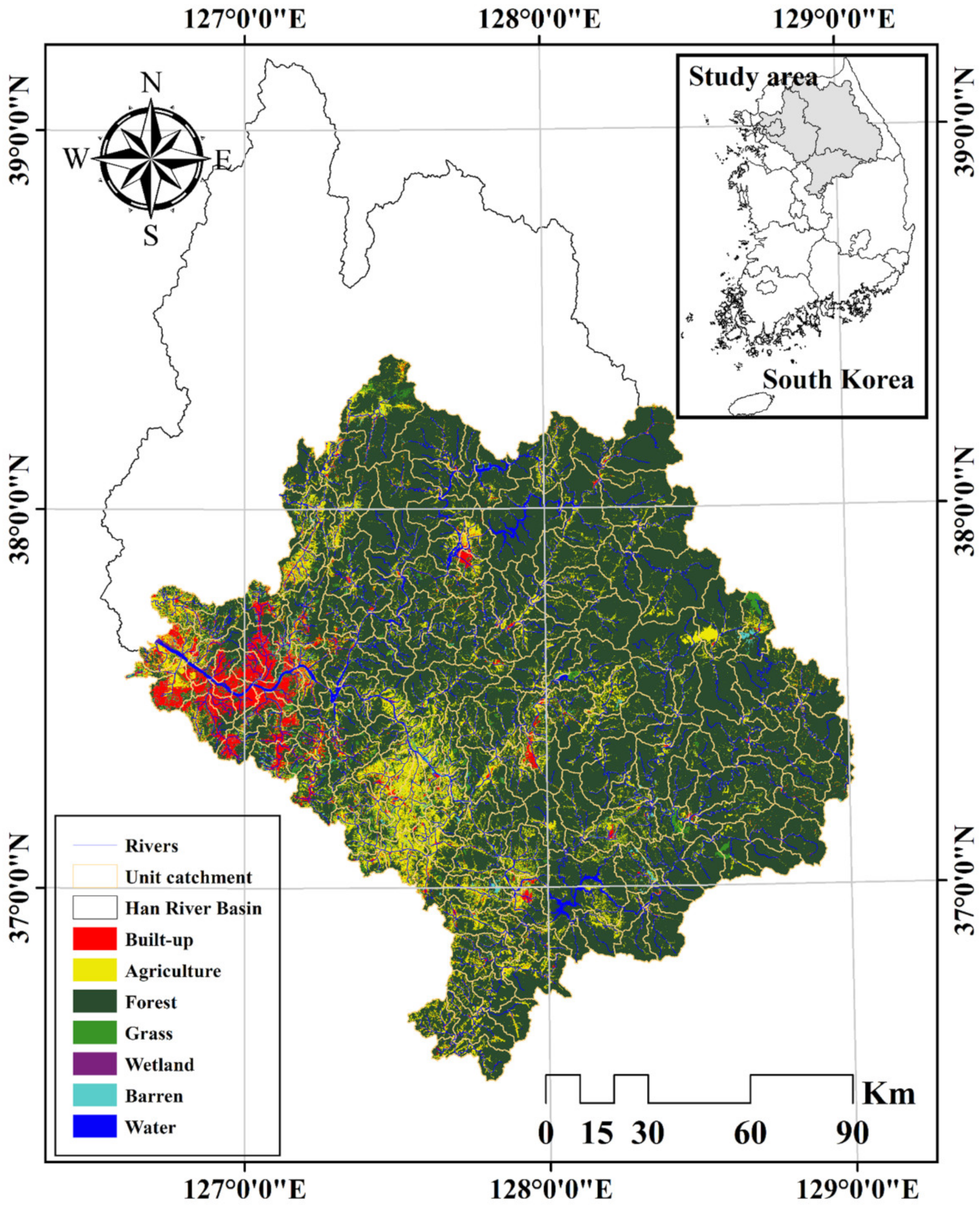
The Han River basin in Korea, which consists of 24 sub-basins and 237 unit catchments (Figure 1), was selected as the study area. Among the 24 sub-basins, 7 sub-basins and 54 unit catchments are located in North Korea, making it difficult to obtain data; therefore, only 183 unit catchments were used for analysis. Within the basin, there are 48 flow measurement points of the Ministry of Environment (MOE) in Korea and 27 meteorological stations of the Meteorological Administration. The flow measurement data for 2011–2015 were collected and used to calibrate the hydrological model. Meteorological observation data were collected for 1970–2015 and were used for hydrological modeling, and potential evapotranspiration and aridity index calculation, etc.

Table 1. Summary characteristics of 183 catchments.

Watershed Characteristics	Min	Max	Average	Standard Deviation
Annual average precipitation (mm)	586.8	2991.8	1291.8	346.8
Annual average evapotranspiration (mm)	675.7	1103.8	850.4	64.3
Aridity index (PE/P)	0.2	1.8	0.7	0.2
Watershed area (km2)	39.2	449.5	126.9	66.9
Built-up (%)	0.2	70.1	7.7	13.5
Agriculture (%)	0.0	60.8	14.5	10.8
Forest (%)	2.9	96.6	68.5	21.2
Grass (%)	0.0	16.8	3.7	2.6
Wetland (%)	0.0	13.8	0.7	1.1
Barren (%)	0.1	59.1	2.5	5.5
Water (%)	0.1	20.4	2.5	3.3

presents a summary of characteristics in the 183 unit catchments. Potential evapotranspiration was calculated using the FAO-56 Penman–Monteith equation. The range of aridity index was 0.2–1.8, with an average of 0.7. The climate of the study site, which was classified according to the criteria in a previous study [25], was humid or semi-humid. The watershed area was 39.2–449.75 km², which was smaller than those in previous studies [22,23,24]. For the land use, the data from the MOE created in 2013 were used. The unit catchment located in the upper reaches of the Han River basin has a high proportion of forests, while that located downstream is urbanized. In the Han River basin middle stream, several unit catchments with a high proportion of agricultural areas are distributed. As such, the Han River basin is suitable for analyzing various land-use type watersheds.

2.2. HSPF Simulation for Data Source of Basin-Specific Budyko Parameters

To derive basin-specific Budyko parameters, calculating AE/P from long-term runoff or actual evaporation data according to weather conditions is necessary in the same watershed environment. However, flow rate observation points are not located within all unit catchments in the study site. Moreover, AE is challenging to predict due to vegetation change; due to the heterogeneity of the basin environment, such as land use and vegetation change, the value of w of the Budyko parameter changes annually. In the present study, HSPF was used to make up for insufficient data and derive highly accurate basin-specific w values for the current status of the basin.

HSPF is a process-based, conceptual, and continuous simulation watershed model for quantifying hydrology and water quality. It can simulate runoff and pollutant loadings for watersheds and perform flow and water quality routing in the watershed reaches [26,27]. HSPF uses time-series data such as rainfall, temperature, and solar radiation as well as land-use data such as land-use patterns and land management practices [28]. HSPF has three modules: pervious land segment, impervious land segment, and free-flowing reach [26,27]. HSPF computes hydrological cycle components (evapotranspiration, surface detention, surface runoff, infiltration, interflow, base flow, and percolation to deep groundwater) in the pervious land segment. It only computes surface components of the hydrological cycle in the impervious land segment, while in the free-flowing reach, HSPF computes hydraulic behavior using kinematic assumption.

Sub-watershed, topographic, and hydrological data were constructed for use in the simulation of HSPF (Figure 1). A sub-watershed is a unit catchment that has been partially divided for calibration. Topographic data are used for the digital elevation model (DEM) and land-use map, following the conversion of altitude img files provided by the National Geographic Information Institute (NGII) into a grid (10 m × 10 m). Land use was constructed with data provided by the MOE as of 2013 and classified into seven land-use types (

Table 2. Classification and description of land-use data.

Classification	Description
Built-up	Buildings such as residential facilities, commercial and industrial facilities, and transportation facilities
Agriculture	Agricultural areas for plowing paddy fields and upland, areas for cultivating fruit trees and street trees, and facilities used for livestock and dairy farming
Forest	Land where trees grow collectively
Grass	Land covered with herbaceous plants, natural grasslands, and artificial grasslands formed
Wetland	Moist and humid land where moisture is always maintained by the natural environment
Barren	Bare ground with no vegetation cover
Water	Low areas with pooled water, such as lakes, reservoirs, and swamps

). Weather data were constructed as hydrological data from 1970 to 2015 observed at the automated surface observing systems (ASOS) site, such as precipitation, average temperature, and insolation. Moreover, to reflect the artificial flow, dams, beams, and sewage treatment plant discharge data from 2010 to 2014 were used.

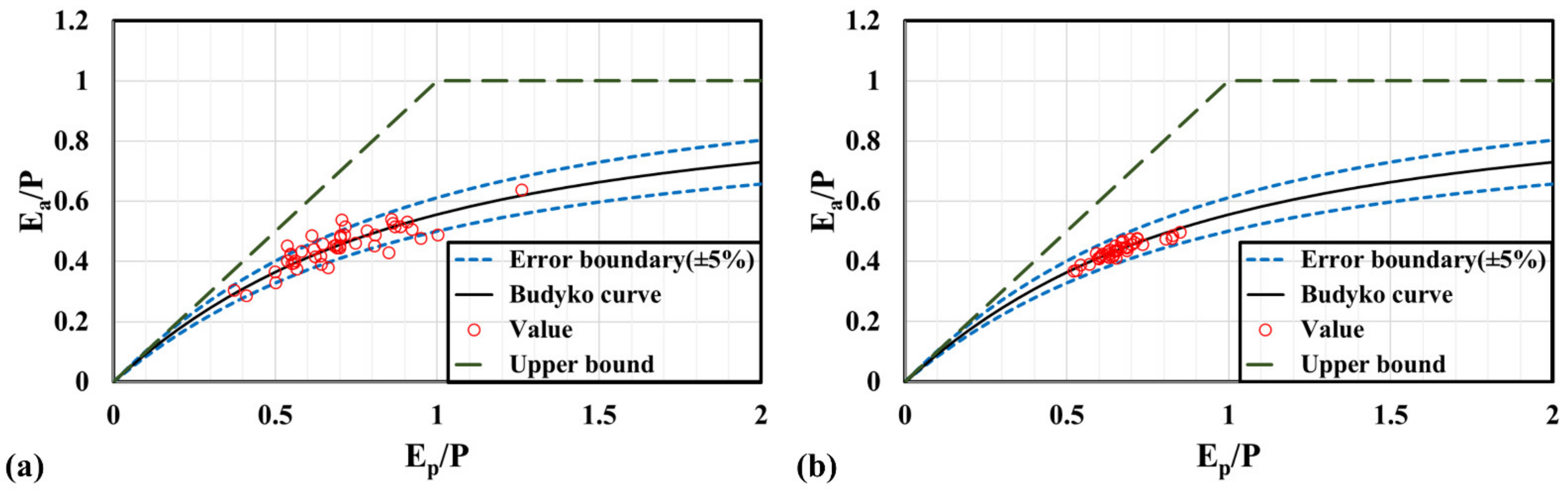
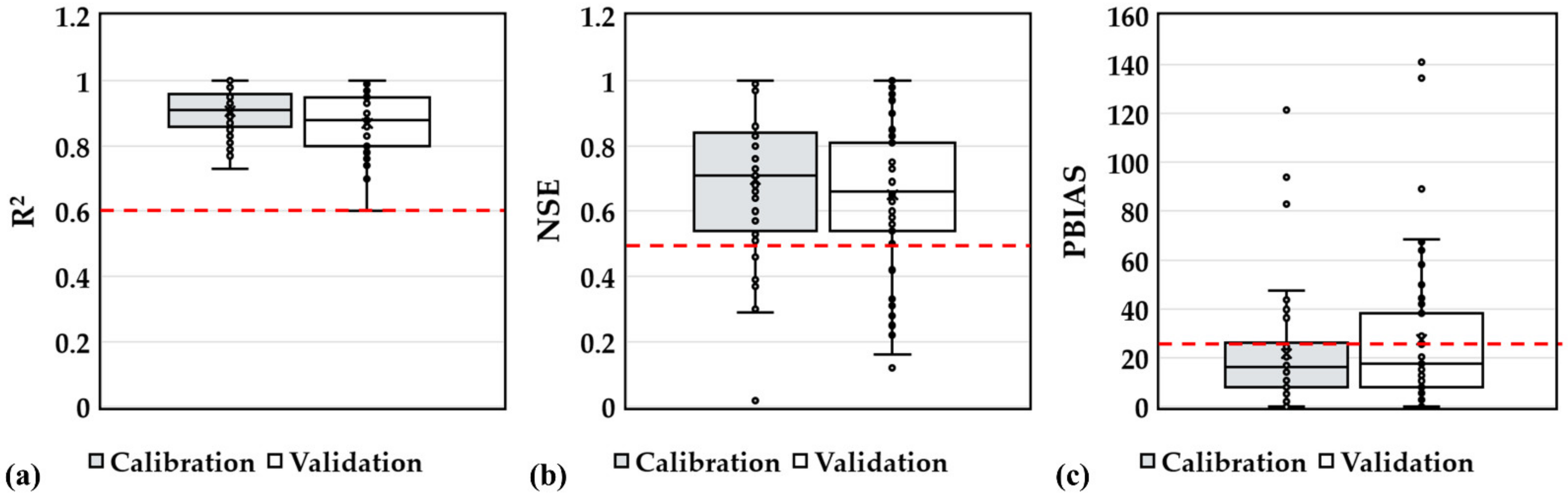
The model was calibrated and validated using the trial and error method for 48 points, and observed data were acquired using the water resources management information system (WAMIS). Calibration of the model was performed for 2010–2012, and validation was done for 2013–2014. For the evaluation of the calibrated results, the criteria proposed by [29] were applied, which are shown in

Table 3. Performance evaluation criteria for recommended statistical performance measure for a watershed-scale model [29].

Statistical Indicator	Performance Evaluation Criteria
	Very Good	Good	Satisfactory	Not Satisfactory
R2	R2 > 0.85	0.75 < R2 ≤ 0.85	0.60 < R2 ≤ 0.75	R2 ≤ 0.60
NSE	NSE > 0.75	0.65 < NSE ≤ 0.75	0.50 < NSE ≤ 0.65	NSE ≤ 0.50
PBIAS	PBIAS < ±10	±10 ≤ PBIAS < ±15	±15 ≤ PBIAS < ±25	PBIAS ≥ ±25

.

2.3. w Estimated Model Development and Watershed Quality Criteria Established

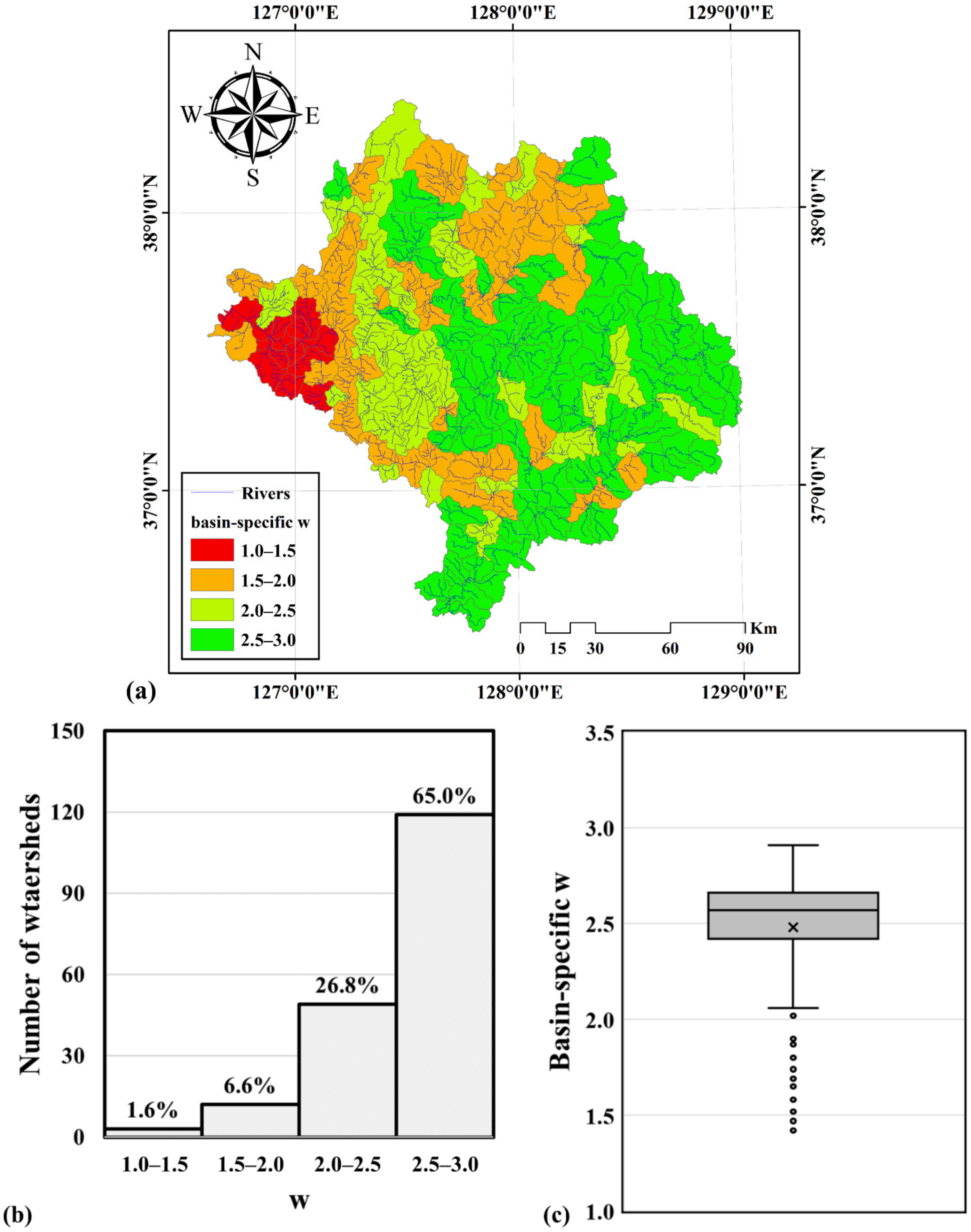
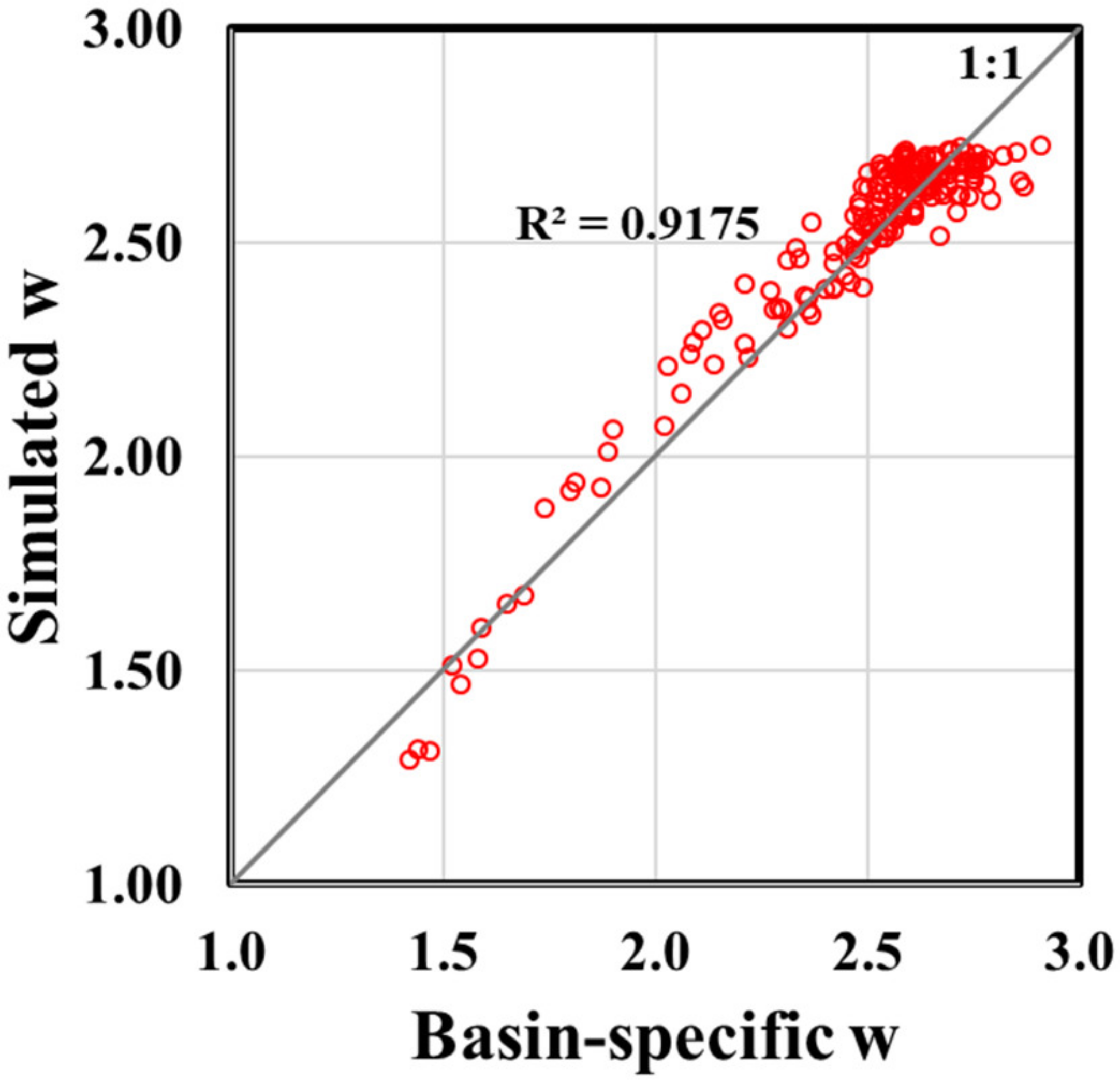
The Budyko parameter for each watershed (basin-specific w) was corrected to minimize the root mean square error (RMSE) of Budyko-simulated and model-simulated AE/P values on the annual scale. The AE of the model-simulated AE/P was derived as AE = P − Q by assuming P = Q + AE according to the long-term water-energy balance at the basin scale. Data from 1970 to 2015 were used, and basin-specific w of 183 watersheds was derived.

The w estimation model was developed using stepwise multiple regression analysis to evaluate change in w due to changes in the watershed environment. As an independent variable for estimating w, the area ratios of the seven land-use classifications in Table 2 were used, and data from 183 watersheds were used for the multiple regression analysis.

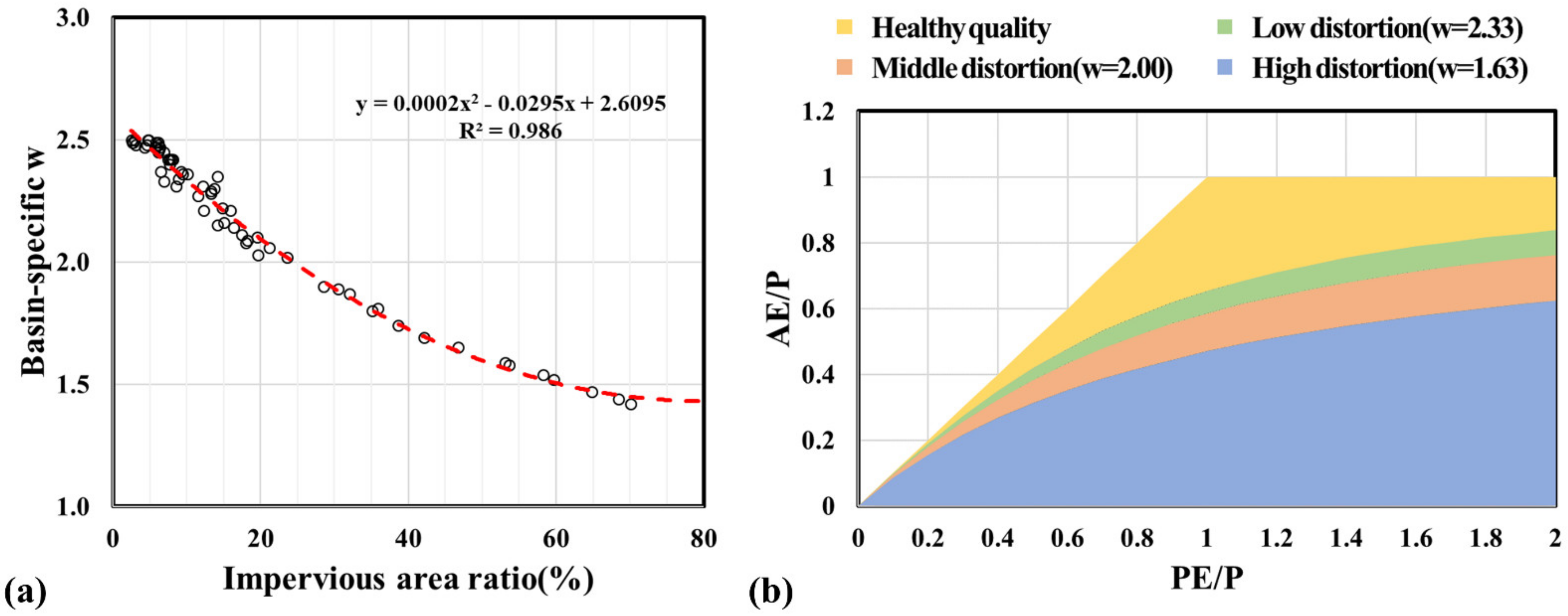
Correlation and cluster analyses were used to develop watershed quality evaluation criteria using w. Pearson correlation analysis was performed to extract factors with a high correlation with w, and factors with high correlation were used for cluster analysis. Cluster analysis was used to create classes for classifying watershed quality. An appropriate number of clusters was derived from a dendrogram, and K-means cluster analysis was performed according to the number.

2.4. HSPF LID Tool for Watershed Quality Criteria Applicability Assessment

The applicability of watershed quality criteria was analyzed using HSPF applied to the watershed management technique. HSPF’s low impact development (LID) Tool was used, and the Gulpocheon unit catchment with a large change in w in 2013 compared to that in 1975 was selected as the study area. The LID was applied to the calibrated HSPF, and the runoff was calculated. The LID tool has been used in many studies, and a detailed explanation is described in the study of Mohamoud et al. [30].

3. Results

3.1. HSPF Calibration and Validation

The parameters of HSPF were calibrated and validated at 48 flow measurement points. The parameters shown in

Table 4. Hydrological Simulation Program-Fortran (HSPF) parameters related to runoff simulation and calibrated value.

Parameter		Initial Value	Calibrated Value	Explanation	Unit
PWAT-PARM2	LZSN	4.0–6.5	4.0–6.5	lower zone nominal soil moisture storage	inches
	INFILT	0.16	0.01–0.30	index to infiltration capacity	in/h
	LSUR	150–250	150–350	Length of overland flow	feet
	KVARY	0	0.0–3.0	Variable groundwater recession	1/inches
	AGWRC	0.98	0.920–0.998	Base groundwater recession	none
	SLSUR	-	0.001–0.885	Slope of overland flow plane	none
PWAT-PARM3	DEEPFR	0.1	0.00–0.45	Fraction of GW inflow to deep recharge	none
	BASETP	0.02	0.01–0.05	Fraction of remaining ET from baseflow	none
	AGWETP	0	0.0–0.1	Fraction of remaining ET from active GW	none
PWAT-PARM4	UZSN	1.128	0.100–1.228	Upper zone nominal soil moisture storage	none
	INTFW	0.75	3	Interflow inflow parameter	none
	IRC	0.5	0.5–0.8	Interflow recession parameter	none

were calibrated using trial and error methods, and SLSUR was applied by calculating the slope for each land use of the sub-watershed with DEM. To properly simulate the infiltration, parameters considering the area and infiltration rate of hydrological soil groups were used for INFILT using the soil map of the National Institute of Agricultural Science (NIAS). For statistical variables such as R², NSE, and PBIAS, most watersheds were better than or equal to the “Satisfactory” criteria proposed by [29] (Figure 2). The “Not Satisfactory” criterion was associated with some watersheds for some indicators. However, the remaining indicators appeared as “Satisfactory”, and for one of the calibration or calibration periods, “Satisfactory” appeared, and parameter calibration was deemed to be well done.

3.2. Basin-Specific w Estimation

The runoff data from 1970–2015 were simulated using the calibrated model. AE/P was calculated annually for each watershed using the AE = P − Q equation. AE/P was found to be in the 0.2–0.9 range with an average of 0.5. If the unique characteristics of the watershed do not change due to human activity, the water and energy balance of the watershed is maintained. In other words, the water balance simulated by the hydrological model to which the same land use is applied must move on a constant Budyko curve every year. In particular, the water balance in the watershed is generally closed at the annual level; therefore, it must move on a basin-specific Budyko curve in the annual analysis. However, since quantifying hydrological circulation accurately is challenging, annual results cannot be accurately positioned on the basin-specific Budyko curve even in the annual analysis [31]. In the present study, however, the time scale of the water balance analysis was set from 1 year to 10 years to reduce the error. The longer the time scale, the lower the error rate, and the maximum error rate is less than 10% for time scales of ≥5 years (

Table 5. Number of watersheds within the maximum error rate range of the Budyko curve time scale.

Time Scale	<5%	5–10%	10–15%	>15%	Time Scale	< 5%	5–10%	10–15%	>15%
1 year	0	1	2	180	6 year	92	91	0	0
2 year	0	45	130	8	7 year	61	122	0	0
3 year	1	155	26	1	8 year	63	120	0	0
4 year	10	141	32	0	9 year	91	92	0	0
5 year	54	129	0	0	10 year	146	37	0	0

and Figure 3). In the present study, five years was selected as the time scale.

The basin-specific w for each watershed was estimated by converting the 45-year modeled data of 183 watersheds into the 5-year average. It was found that 65.0% of the total watersheds were in the 2.5–3.0 range, 26.8% were in the 2.0–2.5 range, and 8.2% were in the 1.0–2.0 range (Figure 4). A previous study [24] conducted on 206 watersheds in China revealed that the most distributed watersheds were in the 1.5–2.0 range, followed by 2.0–2.5 and 2.5–3.0, showing different trends from the one observed in the present study. This is thought to be due to the higher annual average precipitation, smaller dryness index, and smaller watershed area. In the present study, the range of w was 1.42–2.91. Peng et al. [24] reported the w range as 1.3–4.9, and Zhang et al. [19] reported the w range as 1.7–5.0. Therefore, the w calculated in this study fell within the w range calculated in previous studies. Meanwhile, Zhang et al. [19] reported that the average w of the forest watershed was 2.84, and in the present study, most of the watersheds with w values of 2.5–3.0 had forest area ratios of almost 80%. The results of the present study are consistent with the trends reported in prior research. The average w was 2.48, and the median value was 2.57. Considering the original Budyko curve default w of Fu [17] was 2.6, the w value corrected by Zhang et al. [19] was 2.63, and the mean w value of Xu et al. [23] was 2.5, the mean of w in the present study was similar to that of previous studies. Moreover, it has been reported that the smaller the watershed area, the smaller the deviation of w [23]. In the present study, the deviation (0.30) of w was low because it was studied on a watershed relatively smaller than that of previous studies.

3.3. Estimation Model for w

w is reportedly affected by land surface characteristics, vegetation, soil types, and topography, and estimation models were developed in consideration of some characteristics [19,20,22,23,24]. Such models were developed with a normalized difference vegetation index (NDVI) as the main factor, and some watershed characteristics were added. Furthermore, since obtaining data for estimating w in small watersheds is challenging, it was developed for large watersheds. As a result, the accuracy of the model reduced as the size of the watershed decreased [22]. In the present study, land-use data were used as they are easy to acquire, and their resolution is low, so that accuracy can be improved even in small watersheds. The relationship between land-use area ratio and w was analyzed, and a w estimation model was developed. As a result of the correlation analysis between w and land-use area, w had a high negative correlation (−0.946) with the built-up area ratio and a high positive correlation (0.790) with the forest (

Table 6. Pearson correlation analysis result of w and land-use area ratio.

Parameter	Built-Up	Agriculture	Forest	Grass	Wetland	Barren	Water
w	−0.946 **	−0.058	0.790 **	−0.513 **	0.072	−0.241 **	−0.312 **

** The correlation is significant at the 0.01 level (bilateral).

). Other factors such as grass, water, and barren areas also had high correlations with the characteristics of Peng et al. [24]. Land-use area ratio could be used in the regression model for w estimation. The model used multiple linear regression (MLR) analysis techniques, and a regression model for w estimation was derived by performing stepwise multiple regression analysis. Land use for predicting w was selected from built-up, forest, grass, and wetlands, and the estimated regression equation is as follows:

w (simulated w) = 2.444 − 0.017 × Built-up (%) + 0.003 × Forest (%) − 0.007 × Grass (%) + 0.013 × Wetland (%)

(3)

For simulated w and basin-specific w, R² was 0.918, and the RMSE was 0.088, indicating that the regression model-simulated w had a good fit (Figure 5).

3.4. Establishment and Application of Watershed Quality Criteria

3.4.1. Establishment of Watershed Quality Criteria

To use the Budyko parameter w as the criterion for evaluating the watershed hydrological system, we tried to establish a standard based on the relationship with impervious area ratio, which is reported to be harmful to hydrological systems. The Pearson correlation coefficient between w and the built-up area ratio was highly negative, at −0.946. Since residential, commercial, industrial facilities, and transportation facilities corresponding to the impervious area are included in the built-up area, a direct connection between the two factors indicated it would be possible. A cluster analysis was performed using w and impervious area ratio to create the evaluation criteria. As a result of hierarchical clustering, clusters of six hierarchies were created, and each hierarchical division is shown in

Table 7. Cluster analysis results according to the number of clusters (case).

	Classification	Count	w	Impervious Area Ratio (%)
Case 1	1	3	1.42–1.47	64.80–70.07
	2	5	1.52–1.65	46.71–59.65
	3	7	1.69–1.90	28.48–42.11
	4	18	2.02–2.35	12.21–23.58
	5	35	2.27–2.61	4.26–11.48
	6	115	2.48–2.91	0.21–3.99
Case 2	1	7	1.42–1.59	53.13–70.07
	2	8	1.65–1.90	28.48–46.71
	3	23	2.07–2.37	8.92–23.58
	4	145	2.31–2.91	0.21–8.54

. As a result of cluster analysis, w could be properly classified according to the impervious area ratio. However, since the data used in the analysis were not distributed over all sections, there was a limit to clearly dividing the boundaries among clusters using a specific impervious area ratio.

The evaluation boundary was established using an impervious cover model (ICM) to establish the criteria for the cluster boundary and watershed quality. ICM is a tool for watershed management in urban watersheds developed by Schueler et al. [32,33], which classifies urban rivers into four categories (sensitive, impacted, non-supporting, and urban drainage) according to the impervious area ratio. The clusters between w and impermeable area ratio were adjusted and classified into four categories using the results of previous watershed evaluation studies using ICM. The classification results are represented in case 2 (Table 7). Excluding the examples of clusters 1 and 2, cluster boundaries were similar to those of ICM (0–10, 10–25, 25–60, and 60–100). The four categories for evaluating watershed quality were suggested by combining the two results, as shown in

Table 8. Watershed quality criteria development result.

Watershed Quality	Parameter w	Impervious Area Ratio
High distortion	<1.63	50<
Middle distortion	1.63–2.00	25–50
Low distortion	2.00–2.33	25–10
Healthy quality	2.33<	<10

. The w, which is the boundary of each category, was derived as a quadratic polynomial between w and the impervious area ratio. To improve the prediction accuracy, only w values less than 2.5 were used for data analysis, and the predicted results are shown in Figure 6.

3.4.2. Application of Watershed Quality Criteria

To evaluate the applicability of the developed indicator, change in watershed quality was evaluated by comparing previous and present w values. The w value in the past was used to select the period when the damage caused by the development was low, and 1975 data were calculated as the oldest data among the land-use data provided by the MOE. Land-use data in 1975 were deemed to reflect the state before damage to the watershed because the ratio of built-up was lower than that of the present, and the ratio of agriculture and forest was high (Figure 7).

The w of the study area ranged from −0.72 to 0.20, and decreased by 0.12 on average. Between 1975 and 2013, the grade changed in 31 watersheds, deteriorating in 30 watersheds (

Table 9. The number of watersheds in watershed quality criteria at the past and present.

Watershed Quality	1975	2013
High distortion	2	7
Middle distortion	1	8
Low distortion	5	17
Healthy quality	166	142

). The w in the watershed with deteriorated grades ranged from −0.72 to −0.20 and decreased by 0.47 on average. The w of the grade watersheds with deteriorated grades was 2.40 on average in 1975 but decreased to 2.05 by 2013. In this case, built-up, agriculture, and forest land use increased from 7.86%, 35.16%, and 49.44%, respectively, in 1975, to 28.12%, 15.40%, and 40.43%, respectively, in 2013. It is thought that change in w reflects deterioration in watershed quality due to land-use change.

3.5. Applicability Assessment of Watershed Quality Criteria

Watershed quality grade changes were analyzed by applying watershed management techniques to the evaluation criteria developed in the present study. LID was applied as the watershed management technique, and the LID application scenario was the management of 50% of the built-up area.

Table 10. Changes in characteristics of Gulpocheon unit catchment in the past, present, and after LID.

Category	Past	Present	Watershed Management (LID)
w	2.26	1.58	1.81
Watershed quality	Low distortion	High distortion	Middle distortion
Annual runoff (mm)	530.5	714.3	631.1
Built-up (%)	53.65	13.89
Agriculture (%)	15.60	53.02
Forest (%)	2.80	1.08
Grass (%)	16.95	26.87
Wetland (%)	9.38	4.60
Barren (%)	0.72	0.00
Water (%)	0.90	0.54

shows changes in the past, present, and after LID application. The Gulpocheon basin had a good grade in the past (w = 2.26), which changed to a poor grade in 2015 (w = 1.58). Built-up land use increased from 13.89% in the past to 53.65%, while agriculture decreased from 53.02% to 15.60%; forestland and grassland decreased from 26.87% to 16.75%, and 4.60% to 9.38%, respectively. It was simulated during 1970–2015 to derive accurate w reflecting various weather conditions. As a result of the simulation, the average annual runoff increased from 530.5 mm in the past to 714.3 mm in the present, but decreased to 631.1 mm when LID was applied. w recovered to 1.81, and watershed quality exhibited a poor grade. Therefore, the indicator developed in the present study can derive w from meteorological data and runoff and can be applied in watershed quality evaluation. It also demonstrates that predicting future watershed quality change based on runoff is possible.

4. Conclusions

In the present study, we used the Budyko curve parameters as watershed management indices and attempted to establish watershed quality grades. Fu’s equations for the Budyko curve and a single parameter, w, were used, and basin-specific w was calculated for 183 sub-basins. A w estimation model was developed by multiple regression analysis of land-use data and basin-specific w. Cluster analysis was used to establish watershed quality standards, in addition to a dendrogram and an ICM. Finally, the indicator’s applicability was evaluated by applying the watershed management technique to the hydrological model HSPF.

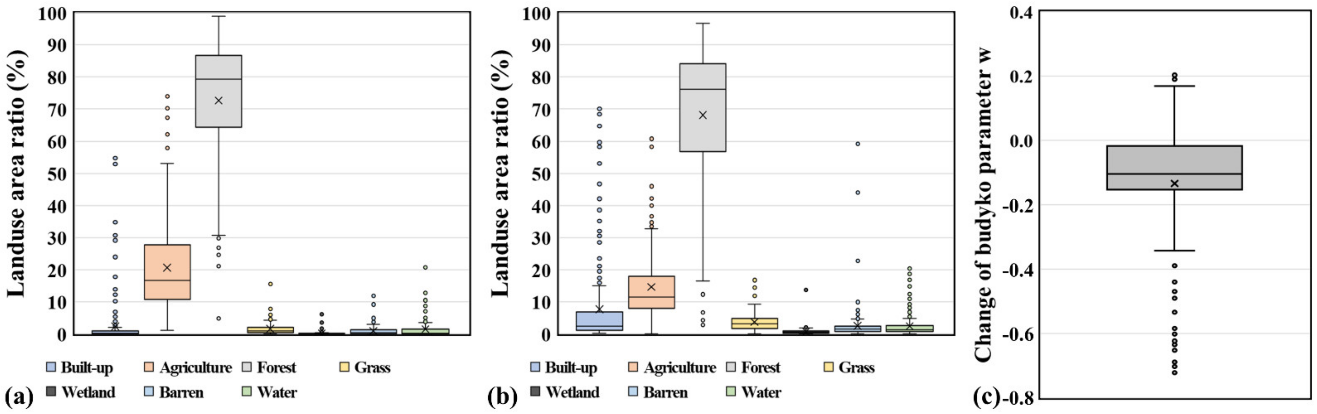
The results of the present study showed that the parameter w of the Budyko curve parameter could facilitate the evaluation of watershed quality. w showed a high correlation with the percentage of land-use area in the watershed, especially with built-up area and forestland uses. Cluster analysis was performed on w with the impervious area ratio, which is related to the built-up area and has been extensively used as a watershed management indicator. Based on the dendrogram and ICM, w was classified into four grades, and changes in watershed quality in the past and present were analyzed. With urbanization, the built-up area ratio increased compared to that of the past, and the watershed quality deteriorated in 31 watersheds. In addition, watershed quality criteria changed with w, which was calculated as a result of the simulation of LID application as a watershed management technique in HSPF. At the same time, we confirmed that w can be used as an indicator for the evaluation of watershed quality in watersheds where the LID technique, which is an example of sustainable development, is applied.

In conclusion, the indicator w developed in the present study can be easily utilized by policymakers for watershed quality assessment and hydrological system identification. Since the watershed quality can be evaluated by the ratio of land-use area, it will be possible to assess the quality in the past and present easily and can be used to predict changes in watershed quality according to the watershed development plans. In addition, since it is possible to evaluate it in connection with hydrological modeling through the application of watershed management techniques, it will be possible to identify changes in watershed quality, including development plans and watershed management plans, and use them to establish optimal strategies for quality improvement. The developed indicator is judged to be a valuable result in that it is possible to easily evaluate only the results of watershed management regardless of the various climates of the hydrology system, which is highly affected by rainfall.

Nevertheless, the indicator in the present study has two limitations. First, in some watersheds, the point on the Budyko curve cannot be determined using the observed stream discharge. Some watersheds have reservoirs and sewage treatment plants, and the flow of streams changes due to the discharge from such facilities. Because the Budyko hypothesis explains natural water-energy balance, the developed indicator did not consider the effect of artificial discharge. Therefore, the current watershed quality cannot be evaluated using the monitored discharge. If the reservoir’s effect is also considered with the model used in other studies [34,35], and the other artificial flow is considered, the indicator is expected to improve. Secondly, complex hydrological modeling was included for evaluation including watershed management plans. If additional elements such as the subdivision of land-use types and the application of LID management areas are supplemented in the indicator estimation model through further research, it would be more effectively used to assess watershed quality.

References

1. Barnett, T.P.; Pierce, D.W.; Hidalgo, H.G.; Bonfils, C.; Santer, B.D.; Das, T.; Bala, G.; Wood, A.W.; Nozawa, T.; Mirin, A.A. Human-induced changes in the hydrology of the western United States. Science 2008, 319, 1080–1083. [Google Scholar] [CrossRef] [Green Version]
2. Milly, P.C.D.; Betancourt, J.; Falkenmark, M.; Hirsch, R.M.; Kundzewicz, Z.W.; Lettenmaier, D.P.; Stouffer, R.J. Stationarity is dead: Whither water management? Science 2008, 319, 573–574. [Google Scholar] [CrossRef]
3. Wagener, T.; Sivapalan, M.; Troch, P.A.; McGlynn, B.L.; Harman, C.J.; Gupta, H.V.; Kumar, P.; Rao, P.S.C.; Basu, N.B.; Wilson, J.S. The future of hydrology: An evolving science for a changing world. Water Resour. Res. 2010, 46. [Google Scholar] [CrossRef]
4. Vogel, R.M. Hydromorphology. Water Resour. Plan. Manag. 2011, 137, 147–149. [Google Scholar] [CrossRef]
5. Wang, D.B.; Mohanmad, H. Quantifying the relative contribution of the climate and direct human impacts on mean annual streamflow in the contiguous United States. Water Resour. Res. 2011, 47. [Google Scholar] [CrossRef] [Green Version]
6. Pumo, D.D.; Arnone, E.; Francipane, A.; Caracciolo, D.; Noto, L.V. Potential implications of climate change and urbanization on watershed hydrology. J. Hydrol. 2017, 554, 80–99. [Google Scholar] [CrossRef]
7. Oudin, L.; Salavati, B.; Furusho-Percot, C.; Ribstein, P.; Saadi, M. Hydrological impacts of urbanization at the catchment scale. J. Hydrol. 2018, 559, 774–786. [Google Scholar] [CrossRef] [Green Version]
8. Olden, J.D.; Poff, N.L. Redundancy and the choice of hydrologic indices for characterizing stream flow regimes. River Res. Appl. 2003, 19, 101–121. [Google Scholar] [CrossRef]
9. Black, A.R.; Rowan, J.S.; Duck, R.W.; Bragg, O.M. DHRAM: A method for classifying river flow regime alterations for the EC Water Framework Directive. Aquat. Conserv. Mar. Freshw. Ecosyst. 2005, 15, 427–446. [Google Scholar] [CrossRef]
10. Gao, Y.; Vogel, R.M.; Kroll, C.N.; Poff, N.L.; Olden, J.D. Development of representative indicators of hydrologic alteration. J. Hydrol. 2009, 374, 136–147. [Google Scholar] [CrossRef]
11. Chaves, H.M.L.; Alipaz, S. An integrated indicator based on basin hydrology, environment, life, and policy: The watershed sustainability index. Water Resour. Manag. 2007, 21, 883–895. [Google Scholar] [CrossRef]
12. Cortés, A.E.; Oyarzún, R.; Kretschmer, N.; Chaves, H.; Soto, G.; Soto, M.; Amézaga, J.; Rötting, T.; Señoret, M.; Maturana, H. Application of the Watershed Sustainability Index to the Elqui river basin, North-Central Chile. Obras Proy. 2012, 12, 57–69. [Google Scholar] [CrossRef] [Green Version]
13. Zhang, Q.; Gu, X.; Singh, V.P.; Chen, X. Evaluation of ecological instream flow using multiple ecological indicators with consideration of hydrological alterations. J. Hydrol. 2015, 529, 711–722. [Google Scholar] [CrossRef]
14. Wang, X. Advances in separating effects of climate variability and human activity on stream discharge: An overview. Adv. Water Resour. 2014, 71, 209–218. [Google Scholar] [CrossRef]
15. Dey, P.; Mishra, A. Separating the impacts of climate change and human activities on streamflow: A review of methodologies and critical assumptions. J. Hydrol. 2017, 548, 278–290. [Google Scholar] [CrossRef]
16. Budyko, M.I. Climate and Life; Academic Press: New York, NY, USA, 1974. [Google Scholar]
17. Fu, B.P. The calculation of the evaporation from land surface. Sci. Atmos. Sin. 1981, 5, 23–31. [Google Scholar]
18. Choudhury, B. Evaluation of an empirical equation for annual evaporation using field observations and results from a biophysical model. J. Hydrol. 1999, 216, 99–110. [Google Scholar] [CrossRef]
19. Zhang, L.; Hickel, K.; Dawes, W.R.; Chiew, F.H.S.; Western, A.W.; Briggs, P.R. A rational function approach for estimating mean annual evapotranspiration. Water Resour. Res. 2004, 40, W02502. [Google Scholar] [CrossRef]
20. Yang, D.; Sun, F.; Liu, Z.; Cong, Z.; Ni, G.; Lei, Z. Analyzing spatial and temporal variability of annual water-energy balance in nonhumid regions of China using the Budyko hypothesis. Water Resour. Res. 2007, 43, 436–451. [Google Scholar] [CrossRef]
21. Yang, D.; Shao, W.; Yeh, P.J.-F.; Yang, H.; Kanae, S.; Oki, T. Impact of vegetation coverage on regional water balance in the nonhumid regions of China. Water Resour. Res. 2009, 45. [Google Scholar] [CrossRef] [Green Version]
22. Li, D.; Pan, M.; Cong, Z.; Zhang, L.; Wood, E. Vegetation control on water and energy balance within the Budyko framework. Water Resour. Res. 2013, 49, 969–976. [Google Scholar] [CrossRef]
23. Xu, X.; Liu, W.; Scanlon, B.R.; Zhang, L.; Pan, M. Local and global factors controlling water-energy balances within the Budyko framework. Geophys. Res. Lett. 2013, 40, 6123–6129. [Google Scholar] [CrossRef]
24. Bai, P.; Liu, X.; Zhang, D.; Liu, C. Estimation of the Budyko model parameter for small basins in China. Hydrol. Process. 2020, 34, 125–138. [Google Scholar] [CrossRef]
25. Huang, H.; Han, Y.; Cao, M.; Song, J.; Xiao, H. Spatial-temporal variation of aridity index of China during 1960–2013. Adv. Meteorol. 2016, 31, 1488–1498. [Google Scholar] [CrossRef]
26. Duda, P.B.; Hummel, P.R.; Donigian, A.S., Jr.; Iimhoff, J.C. BASINS/HSPF: Model Use, Calibration and Validation. Trans. ASABE 2012, 55, 1523–1547. [Google Scholar] [CrossRef]
27. Singh, J.; Knapp, H.V.; Arnold, J.G.; Demissie, M. Hydrological Modeling of the Iroquois River Watershed Using HSPF and SWAT. J. Am. Water Resour. Assoc. 2005, 41, 343–360. [Google Scholar] [CrossRef]
28. Lian, Y.; Chan, I.C.; Xie, H.; Demissie, M. Improving HSPF modeling accuracy from FTABLES: Case study for the Illinois River basin. J. Hydrol. Eng. 2010, 15, 642–650. [Google Scholar] [CrossRef]
29. Moriasi, D.N.; Gitau, M.W.; Pai, N.; Daggupati, P. Hydrologic and water quality models: Performance measures and evaluation criteria. Trans. ASABE 2015, 58, 1763–1785. [Google Scholar]
30. Mohamoud, Y.M.; Parmar, R.S.; Wolfe, K.L.; Carleton, J.N. HSPF Toolkit: A New Tool for Stormwater Management at the Watershed Scale. In Proceedings of the Sustainability 2008—Green Practices for the Water Environment Conference, National Harbor, MD, USA, 22–25 June 2008. [Google Scholar]
31. Gentine, P.; D’Odorico, P.; Lintner, B.R.; Sivandran, G.; Salvucci, G. Interdependence of climate, soil, and vegetation as constrained by the Budyjo curve. Geophys. Res. Lett. 2012, 39, L19404. [Google Scholar] [CrossRef] [Green Version]
32. Schueler, T.R. The importance of imperviousness. Watershed Prot. Tech. 1994, 1, 100–111. [Google Scholar]
33. Schueler, T.R.; Fraley-McNeal, L.; Cappiella, K. Is impervious cover still important? Review of recenty research. J. Hydrol. Eng. 2009, 14, 309–315. [Google Scholar] [CrossRef] [Green Version]
34. Bracht-Flyr, B.; Istanbulluoglu, E.; Fritz, S. A hydro-climatological lake classification model and its evaluation using global data. J. Hydrol. 2013, 486, 376–383. [Google Scholar] [CrossRef] [Green Version]
35. Demertzi, K.; Papadimos, D.; Aschonitis, V.; Papamichail, D. A Simplistic Approach for Assessing Hydroclimatic Vulnerability of Lakes and Reservoirs with Regulated Superficial Outflow. Hydrology 2019, 6, 61. [Google Scholar] [CrossRef] [Green Version]
Figure 1. Locations and land use of the 183 unit catchments in this study.
Sustainability 13 03864 g001
Figure 2. Statistical indices of calibration and validation: (a) R2; (b) Nash-sutcliffe efficiency (NSE); (c) Percent bias (PBIAS).
Sustainability 13 03864 g002
Figure 3. Variation of Budyko curve values according to time scale for water balance analysis: (a) Time scale—1 year; (b) Time scale—5 year.
Sustainability 13 03864 g003
Figure 4. (a) Spatial distribution of basin-specific w in Han River basin; (b) frequency histogram of the basin-specific w in 183 unit catchment; (c) box-plot of the basin-specific w in 183 unit catchment.
Sustainability 13 03864 g004
Figure 5. Analysis of the relationship between simulated w by MLR model and basin-specific w.
Sustainability 13 03864 g005
Figure 6. (a) Relationship between basin-specific w and impervious area ratio for setting watershed quality criteria; (b) Budyko curve area according to watershed quality set in four grades (high distortion, middle distortion, low distortion, healthy quality).
Sustainability 13 03864 g006
Figure 7. (a) Land-use area ratio box-plot by type using land-use data in 1975, (b) land-use area ratio box-plot by type using land-use data in 2013, (c) box-plot of Budyko parameter w variation from 1975 to 2013.
Sustainability 13 03864 g007