Article

Sustainability of Energy-Induced Growth Nexus in Brazil: Do Carbon Emissions and Urbanization Matter?

by
Tomiwa Sunday Adebayo
1,
Abraham Ayobamiji Awosusi
2,
Jamiu Adetola Odugbesan
1,
Gbenga Daniel Akinsola
3,
Wing-Keung Wong
4,5,6 and
Husam Rjoub
7,*
1
Department of Business Administration, Faculty of Economics and Administrative Science, Cyprus International University, 99040 Nicosia, Turkey
2
Department of Economics, Faculty of Economics and Administrative Science, Near East University, 99138 Nicosia, Turkey
3
Department of Business Management, Faculty of Economics and Administrative Sciences, Girne American University, 99300 Mersin, Turkey
4
Department of Finance, Fintech & Blockchain Research Center, and Big Data Research Center, Asia University, Taichung City 41354, Taiwan
5
Department of Medical Research, China Medical University, Taichung City 40447, Taiwan
6
Department of Economics and Finance, The Hang Seng University of Hong Kong, Siu Lek Yuen 41354, Hong Kong, China
7
Department of Accounting and Finance, Faculty of Economics and Administrative Sciences, Cyprus International University, Mersin 10, 99040 Haspolat, Turkey
*
Author to whom correspondence should be addressed.
Sustainability 2021, 13(8), 4371; https://0-doi-org.brum.beds.ac.uk/10.3390/su13084371
Submission received: 18 March 2021 / Revised: 6 April 2021 / Accepted: 6 April 2021 / Published: 14 April 2021

Abstract

:
This study assesses the relationship between economic performance and environmental sustainability by taking into account the role of energy consumption, urbanization, and trade openness in Brazil by using data spanning from 1965 to 2019. The study is distinct from previously documented studies in literature in terms of scope for Brazil, where few entries have been recorded. The major objectives are to address the questions: (a) Is there a long-run connection between the variables under consideration? (b) Can CO2 emissions, trade openness, and energy consumption predict economic performance of Brazil? (c) What is the connection between economic growth and the independent variables at different frequencies and time-period? Furthermore, the study utilized dynamic ordinary least square (DOLS), fully modified ordinary least square (FMOLS), Maki Cointegration, and autoregressive distributed lag (ARDL) to capture the long-run association between the variables of interest. Also, we used the Wavelet coherence and Gradual-shift causality tests to capture the causal linkage between economic growth and the regressors. The advantage of the wavelet coherence test is that it can capture causal linkage between series at different frequencies and periods. The outcome of both Maki cointegration and ARDL bounds testing to cointegration affirms the presence of long-run interaction among the parameters of interest. Furthermore, the outcomes of the DOLS and FMOLS revealed that energy consumption, CO2 emissions, and urbanization exert positive impacts on economic growth in Brazil while there is no significant connection between trade openness and economic growth. Moreover, Gradual shift causality test outcomes disclosed that urbanization, trade openness, CO2 emissions and energy usage can predict the economic performance of Brazil. The outcomes of the wavelet coherence test give credence to the FMOLS, DOLS, and Gradual shift causality tests.

1. Introduction

Both industrialized and emerging economies share the aim of achieving economic growth and sustainable development. Despite this drive, several roadblocks stand in the way of achieving such a target. Although environmental deterioration is the most widely argued challenge to achieving the required degree of sustainable development, the association between environmental degradation and economic growth is complex [1]. Environmental deterioration is growing as a consequence of global warming and climate change induced by greenhouse gas (GHG) emissions vis-à-vis CO2 emissions [2,3,4], which has culminated in a myriad of issues like reduced air and water quality, low life expectancy, high child and maternal mortality, and desert incursion. There is strong proof of global warming and climate change all around the planet, and the African continent is not resistant to the latest upsurge of global warming.
Stern et al. [4] opined that GHGs will double by 2035 from the pre-industrial level if adequate actions are not taken. Despite the commitment to control GHGs emissions, the world has not been successful. For instance, the International Energy Agency [5] estimated that carbon dioxide (CO2) emitted constitutes the most significant component of GHG pollution which increased 1.7% by 2018. This record can be traced to the upsurge of the global economy and recent global trends, in combination with higher energy usage. The reality of global warming has become an externality that will have a long time effect on the future of the world. There have been several intergovernmental frameworks implemented to alleviate the disastrous impact of climate change, such as the Kyoto Protocol in Japan and the Paris Agreement in 2015 in France [1,6,7,8,9]. Brazil has the biggest economy in South America, with GDP and GDP Per Capita of US$1.84 trillion and US$8717.19, respectively [10]. When it comes to coping with climate change, Brazil has a special set of conditions. The forestry sector and land-use change are by far the largest sources of pollution in this region, which is home to most of the Amazon. Brazil also utilizes a lot of biofuels in its transportation and gets over 70% of its energy from hydropower. Brazil is one of the five big developing “BRICS” markets, with the sixth highest greenhouse gas (GHG) emissions in the globe. Brazil joined the Paris accord in September 2016. The country’s NDC is targeted at reducing 37% of its 2005 emitted GHG level by 2025. In the run-up to the Paris climate change conference, Brazil raised the commitment of its climate efforts [11]. Nevertheless, recent developments in Brazil, such as a severe economic crisis, massive government bribery scandal, and presidential indictment have raised fears that progress on environment and energy reform is halting. Figure 1 depicts the share of the energy mix for Brazil in 2019. The energy mix of Brazil in 2019 as depicted in Figure 1 comprises oil (38.14%), hydro (28.70%), gas (10.39%), coal (5.29%), wind (4.01%), other renewable energy sources (4.04%), solar (1.16%), and solar (0.40%), respectively [12,13]. The country’s NDC is targeted at reducing 37% of its 2005 emitted GHG level by 2025.
In both theoretical and empirical studies, the effect of trade on GDP remains an area of continuous debate. The lack of consensus was a feature in the contemporary theory framework. Logically, trade is anticipated to impact to economic growth positively [6,8]. Nonetheless, some empirical studies found insignificant connection between trade and economic growth [14,15]. Meanwhile, Adhikary [16] demonstrated a negative interconnection between GDP and trade. In addition, Buhari et al. [17] argued that the connection between economic growth and trade revealed is determined by factors such as the size of the economy and its development level.
Furthermore, increasing population of urban cities especially in emerging countries has led to a strong policy regarding the connection between urbanization and growth [9,18]. The contributions of urban cities to advanced economic growth have drawn the interest of many researchers. However, crucial questions arising on whether rapid urbanization increases the standard of living without causing environmental degradation. The urbanization trends and the essence of development are given inadequate consideration, including sustaining growth and environmental quality. Thus, the mixed findings in the ongoing literature warrant further studies.
It is critical to understand that, as one of the world’s fastest-growing economies, it is imperative to investigate the economy and make relevant economic sustainability recommendations based on empirical findings. A thorough review of the Brazilian economy’s sustainability centered on the findings would enable us to establish effective initiatives to resolve questions such as (a) Will Brazil diversify its energy policies by adopting renewable energy to improve its sustainable economy? (b) Do utilization of energy and trade openness improve economic performance of Brazil? It is also important to note that as Brazil’s economy expands, the country’s place in world CO2 rankings is at risk, and CO2 emissions levels are growing at the same pace as those of other big global emitters including Russia, South Korea, the United States, Japan, and Germany. Nonetheless, given the rapid pace of population development, substantial attempts have been made to mitigate the negative effects of global warming while maintaining GDP growth. This is what inspired the investigators to delve at the variables examined in this study, with the intention of utilizing the results to provide policy suggestions to various policymakers.
This research contributes to the literature by applying the novel wavelet coherence test to investigate the dynamics between variables of interest. The advantage of the wavelet test is that it can capture correlation and causal interconnection between series. To the understanding of the investigators, prior studies did not utilize this technique to assess the connection between these economic indicators. Thus, the present study fills the gap in the ongoing literature. Additionally, the outcomes of this research will be beneficial to policymakers in designing an energy-induced and growth-related policy that will improve environmental sustainability. Thus, the research assesses the impact of urbanization, trade, CO2 emissions, and energy consumption on GDP growth in Brazil.
The organization of the study is as follows: Section 2 presents synopsis of prior studies; Data and methodology are presented in Section 3; Section 4 presents empirical analyses and discussion; Section 5 depicts conclusion and policy recommendation.

2. Literature Review

This section portrays prior studies that analyzed the association between GDP and its regressors: CO2 emissions, urbanization, energy consumption, and trade openness.

2.1. Economic Growth and CO2 Emission Relationship

Bouznit and Pablo-Romero [19] scrutinized the association between GDP and CO2 emissions for Algeria, within the timeframe of 1970 and 2010. The result shows a positive linkage between GDP and CO2 emissions.The study of Lacheheb et al. [20] in Algeria also disclosed positive interconnection between economic growth and CO2 emissions. Bastola and Sapkota [21] assessed the causal interaction between GDP and pollutants in Nepal, employing the Autoregressive distributed lag modelARDL and Johansen cointegration for data covering the period from 1980 to 2011. The result shows a one-way causal from GDP and CO2 emissions. The dynamic panel threshold framework was employed by Aye and Edoja [22] to examine the link between GDP and CO2 for 31 developing economies. The result shows that for a low growth regime, there is a negative linkage between CO2 emissions and GDP while for a high growth regime, there is a positive linkage between GDP and CO2 emissions exists. For MENA nations, Gorus and Aydin [23] also employed the panel data spanning from 1975 to 2014 to scrutinize the interaction between CO2 and GDP. The result shows no causal interaction between CO2 emissionsand GDP. This outcome was also supported by the study of Wang et al. [24] in China. Moreover, Muhammad [25] examined the interaction between GDP and CO2 emissions for 68 nations for the period 2001 to 2017. The 68 countries consist of developed, emerging, and MENA countries. The empirical outcome shows that GDP positively influences CO2 in developed and MENA nations, which is in consonance with the study done by Kirikkaleliand Adebayo [26] for India and He et al. [27] for Mexico. Khobaiand Le Roux [28] scrutinized the interaction between CO2 emissions and GDP growth in South Africa and the outcomes disclosed a unidirectional causal connection from CO2 emissions to GDP which is consistent with the research of Salahuddin et al. [29], Awosusi et al. [30], and Kalmaz, and Adebayo [31], respectively. Acheampong [32] scrutinizes the interconnection between CO2 emissionsand GDP for 116 nations spanning the period 1990 to 2014. The empirical outcomes show no causal interaction between GDP and CO2 emissions but for Latin America and Caribbean region, there is evidence of a negative association between CO2 emissions and economic growth, while in other regions, the association is positive. Mikayilov et al. [33] utilized a multivariate approach to analyze the interaction between GDP and CO2 in Azerbaijan covering the period 1992 to 2013. The empirical outcome shows that the association between GDP and CO2 is positive in Azerbaijan, which agrees with the study done by Adebayo and Odugbesan [7] for South Africa. For 58 countries, Saidi and Hammami [34] employed the GMM technique to uncover a positive interaction between CO2 emissionsand real growth. The study of Begum et al. [35] disclosed a positive connection between GDP and CO2 pollution, which is consistent with the research of Zhang et al. [36] for Malaysia. For BRICS economies, Adedoyin et al. [37] reported a positive interaction between economic growth and CO2 emissions. Meanwhile, Balsalobre-Lorente et al. [38] reported an N-shaped interaction between economic growth and CO2 emissions in 5 European countries. Chen et al. [39] establish positive interaction between GDP and CO2 but the degree of impact differs. Ahmad and Du [40] found a positive linkage between GDP and CO2 in Iran for the period 1971 to 2011.

2.2. Economic Growth and Energy Consumption Relationship

For Nepal, Bouznit and Pablo-Romero [19] revealed a one-way causality interaction from economic growth to energy consumption. The authors assert that policies formulated toward boosting energy consumption cannot promote GDP. Gorus and Aydin [23] assessed the interaction between GDP and energy consumption for MENA nations, utilizing data ranging from 1975 to 2014. The result shows that energy usage Granger cause GDP. Furthermore, in the long run, a negative connection was established but in the short and medium run, the effect is a positive. Khobai and Le Roux [28] scrutinized the causal interaction between GDP and energy consumption in South Africa. The result reveals a two-way causal interconnection between economic growth and energy consumption, which was supported by the study of Wang et al. [24]. Using PVAR and GMM, Acheampong [32] explores the interaction between GDP and energy consumption for 116 nations. The results disclosed no proof of causal interconnection between GDP and energy consumption. Aslan et al. [41] reported a negative interaction between economic growth and energy consumption in G-8 nations. For sub-Saharan Africa, the connection between GDP and energy consumption is positive but the linkage between energy consumption and GDP is negative for Latin America, Caribbean nations, MENA countries, Asia and Pacific nations. Muhammad [25] examined the interaction between energy consumption and GDP for 68 countries for the period 2001 to 2017 using the GMM and seemingly unrelated regression (SUR). The outcome reveals that the connection between energy consumption and GDP is positive in developed and emerging nations but there is negative association in MENA countries. Chen et al. [39] utilized the VECM to scrutinize the interconnection between economic growth and energy usage in 188 countries covering the period from 1993 to 2010. The empirical result reveals a negative association between economic growth and energy usage at the global level and in developing countries while there is no association between GDP and energy usage in developed countries. In Iran, Ahmad and Du [40] found a positive interaction between economic growth and energy usage. Gökmenoğlu and Taspinar [42] found a unidirectional causal linkage between economic growth and energy usage in Turkey. Gozgor et al. [43] utilized the PARDL to scrutinize the relationship between GDP and energy usage for OECD nations. The authors assert that energy consumption is positively related to GDP. The study of Baz et al. [44] disclosed unidirectional causality from energy consumption usage to real growth. Furthermore, Le [45] found a two-way causality between economic growth and energy consumption in 46 nations.

2.3. Economic Growth and Trade Openness Relationship

Iyoha and Okim [16] assessed the connection between trade and GDP in ECOWAS nations from 1990 to 2013 and found a positive connection between trade and GDP. Raghutla [46] found a unidirectional causal association from GDP to trade in emerging economies from 1993 to 2016, which is consistent with the study done by Ahmed [47] for BRICS economies, Le [45] for 46 emerging and developing countries, but the study of Kumari and Malhotra [48] refutes this outcome. The authors assert a bidirectional link between trade and GDP in India. The study of Malefane and Odhiambo [14] disclosed a positive and significant interaction between trade and GDP in Lesotho. Egoro and Obah [49] found a positive interconnection between trade and GDP in Nigeria. Adhikary [15] found a negative interaction between GDP and trade in Bangladesh which implies that trade openness mitigate economic growth. Coulibaly [50] employed the PARDL to examine the association between trade openness and economic growth for 44 sub-Saharan Africa countries, and findings show that the association between trade and GDP is positive. Amna Intisar et al. [51] assessed the interconnection between trade openness and economic growth in Asian nations between 1985 and 2017 and finding confirms a bidirectional causal linkage between trade openness and economic growth in Western Asia, but a one-way causal interconnection from trade openness to GDP was evident in Southern Asia. Zheng and Walsh [52] studied 29 provinces in China and found a mixed outcome.

2.4. Economic Growth and Urbanization Relationship

The study of Nathaniel and Bekun [6] in Nigeria on the interaction between GDP and urbanization employing multivariate technique, and data spanning from 1971 to 2014, revealed a positive interconnection between GDP and urbanization. Another study in Nigeria by Ali et al. [53] established a one-way causal interconnection from urbanization to GDP. This establishes that a significant key contributor to growth in Nigeria is urbanization. Bakirtas and Akpolat [54] examined the causality interaction between GDP and urbanization in emerging economies for the period 1971 to 2014. The result showed a unidirectional causal association from urbanization to GDP. Nguyen [55] investigated ASEAN countries and established a non-linear association between urbanization to GDP. Šatrović and Dağ [56] studied 34 OECD nations from the period from 1996 to 2015 and found a positive interaction between urbanization to GDP. Liddle and Messinis [57] investigated the interaction between urbanization and GDP for 100 countries during the period from 1960 to 2009. These countries were categorized into three based on the income level. For middle-income level countries, it was evident that no causal link between GDP and urbanization. For high-income level countries, a one-way causal interaction from urbanization to GDP whiles a two-way causal interaction between urbanization and GDP in low-income level countries. Solarin et al. [58] scrutinized the connection between GDP and urbanization in Angola using data spanning from 1971 to 2012. The results indicate that urbanization reduces GDP in Angola. In addition, there is one-way causality from urbanization to economic growth in Angola. Table 1 presents summary of related studies.
Based on the reviewed studies, several investigations have been conducted on the association between economic growth, trade openness, CO2 emissions, energy usage, and urbanization. Nonetheless, no prior studies have been conducted investigating these interconnections using the novel wavelet coherence test. The advantage of the wavelet coherence test is that it can capture causal linkage between series at different frequencies and periods.

2.5. Theoretical Framework

This research is constructed on the Environmental Kuznets Curve (EKC), which was originated by Kuznets and Murphy [59] to investigate income inequality. Early scholars like Panayotou [60], Grossman and Krueger [61], and Shafik and Bandyopadhyay [62] followed this theory to scrutinize the effect of economic growth on environmental quality. The EKC is grouped into 3 phases: scale, structural, and composite effects. The scale effect is the first stage, where economic performance is the major priority of the countries without at the expense of environmental quality. This kind of effect is mostly experienced in developing nations whose target is to promote the growth of the economy at the expense of improving her environmental quality. The structural effect is the second stage of the EKC theory, where there is awareness with regards to the impact of their actions on the environment. Economic growth and the environmental quality will at this point be more beneficial, mitigating the consequences of both sides. The composite effect is the final stage, where the majority of the economic activities employed clean technologies that ensure a sustainable economic and environmental quality.

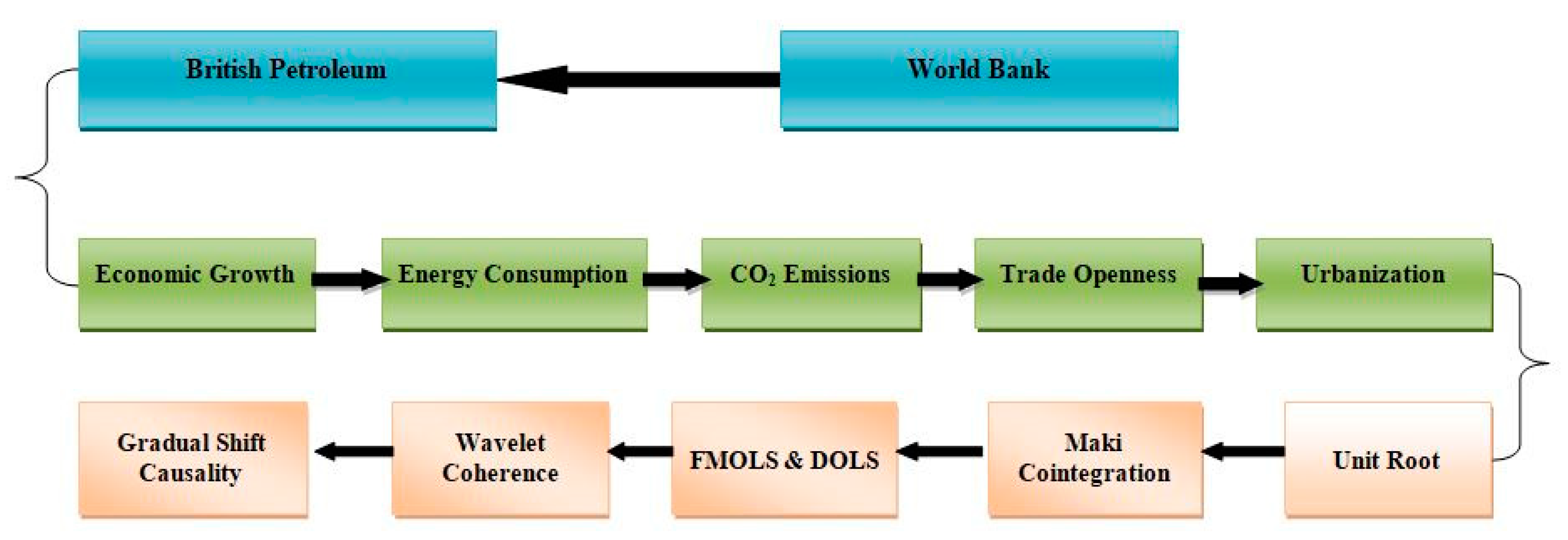
3. Data and Methodology

3.1. Data

This research explores the interaction between CO2 emissions (CO2) and economic growth (GDP) in Brazil, while also accounting for the role of urbanization (URB), trade openness (TR), and energy usage (EC) utilizing data stretching between 1965 and 2019. The empirical modelling is centered on the ARDL technique. This research expands on Nathaniel and Bekun [6] study by including additional growth catalysts ignored in prior literature, such as growth theory triggered by the urban populace. The Solow growth model clearly defines the contribution of labor and capital. For the cases in Brazil that possess similar economic features, urban populations are included in our sample scenario. For the essence of uniformity and the normal distribution, the time series were transmuted to natural logarithm [1,36]. The unit of measurement, sources of the times series and description were clarified in Table 2 and the analysis flow chart is shown in Figure 2. Equations (1) and (2) indicate the economic and econometric model correspondingly.
G D P t = f ( C O 2 t , U R B t , E C t   T R t )
G D P t = ϑ 0 + ϑ 1 C O 2 t + ϑ 2 U R B t + ϑ 3 E C t + ϑ 3 T R t + ε t
In Equation (1), CO2, TR, and EC, URB, and GDP represent CO2 emissions, trade openness, energy usage, urbanization, and economic growth. Additionally, “t” illustrates the study period (1970–2018), the error term is represented by ε , and the parameters are depicted by ϑ 1 ,   ϑ 2 ,   ϑ 3 ,   ϑ 4 ,   and   ϑ 5 .
The present research’s objective is to close this gap in the literature by exploring CO2 emissions (CO2) and GDP in Brazil, while also incorporating the role of energy usage (EN),urbanization (URB), and trade openness (TR) utilizing data stretching between 1965 and 2019. Constant expansion of the economy has contributed to an upsurge in GDP, leading to higher energy demand, which contributes more to emissions [31,63,64]. Furthermore, output expansion and CO2 emissions are positively linked with ecological footprint because of constant natural resource misuse. Thus, CO2 is projected to lead to economic expansion ( β 1 = δ G D P δ C O 2 > 0 ) . Furthermore, authors include that energy usage in the framework in line with the study of Udemba et al. [65], Ali et al. [53], and Bekun and Agboola [66]. Energy usage is anticipated to exert a positive effect on GDP, thus a rise in energy use would increase GDP ( β 2 = G D P E N > 0 ) . In line with the studies of Alam et al. [67], Bekun and Agboola [66], and Ali et al. [53], the current paper introduced urbanization into the model. It is anticipated that urbanization will exert a positive effect on GDP. Hence, a rise in urban population will enhance growth in the economy ( β 3 = G D P U R B > 0 ) . Trade openness was incorporated into the model in line with the studies of AlamandSumon, [68], Kong et al. [69], and Raghutla [46]. The association between trade openness and GDP is anticipated to be positive ( β 4 = G D P T R > 0 ) .

3.2. Methodology

3.2.1. Unit Root Test

This study used the Zivot-Andrews unit root test, proposed by Zivot and Andrews [70], which can detect a stationary property in the presence of a structural break.
Model   A :   Δ y = σ + u ^ y t 1 + β t + γ D U t + j = i t d j Δ y t j +   ε t ,
Model   B :   Δ y = σ + u ^ y t 1 + β t + θ D T t + j = i t d j Δ y t j +   ε t ,
Model   C :   Δ y = σ + u ^ y t 1 + β t + θ D T t γ D U t + j = i t d j Δ y t j +   ε t ,
where: DUt depicts the dummy variable for a mean change that takes place on each potential timebreak (TB); DTt depicts the shift in trend of the variable used. Formally,
D U t = { 1 . i f   t > T B 0 o t h e r w i s e   and   D U t = { t T B i f   t > T B 0 o t h e r w i s e   .

3.2.2. Maki Co-Integration Test

Bearing in mind the structural break (s) in series, the current paper applied Maki co-integration test to explore the cointegration features between CO2, EC, URB, TO, and GDP in Brazil. The study applied this test in contrast to both Hatemi-j [71] and Gregory and Hansen [72] co-integration tests that incorporate breaks because the Maki co-integration test can capture cointegration in series and also captures five breaks simultaneously. The four regression models of the Maki [73] recommendations are stated as follows:
Level shift
Y t = ρ + i = 1 k ρ i D i , t + θ ι Z t + ε t ,
Level shift with trend
Y t = ρ + i = 1 k ρ i D i , t + θ ι Z t + i = 1 k θ ι Z t D i , t + ε t ,
Regime shifts
Y t = ρ + i = 1 k ρ i D i , t + θ ι Z t + σ t + i = 1 k θ ι Z t D i , t + ε t ,
Trend and Regime shifts
Y t = ρ + i = 1 k ρ i D i , t + θ ι Z t + σ t + i = 1 k σ ι D i , t + i = 1 k θ ι Z t D i , t + ε t .
For Equations (7)–(10), subscript t indicate time, which take 1, 2, …, T; Yt denotes dependent variables; Zt denotes independent variables, and ε t denotes error term.

3.2.3. ARDL Approach

The Auto-Regressive Distribution Lag (ARDL) model was employed to capture the long-run cointegration association between the time series. Benefits of the ARDL bounds model over the other conventional or traditional cointegration techniques include: (i) accommodates mixed order of integration [74,75], (ii) it incorporates coefficients in the long and short term simultaneously [74,75], (iii) it is perfectly fit for small sample size [76], (iv) accommodating different lag length [77], and (v) autocorrelation problem is removed. F-distribution and critical value produced by Pesaran and Timmermann [78] and Narayan and Narayan [79] follows the bounds test. The calculated F-statistics is been compared to the critical values (lower and upper) bound. When the calculated F-statistics is below, the null hypothesis is not rejected; the null hypothesis will be rejected when the calculated F-statistics is greater, which shows that long-run connection amongst the variable is evident. Equation (11) below explains the ARDL bounds model:
Δ G D P t = θ 0 + i = 1 t θ 1 Δ G D P t i + i = 1 t θ 2 Δ C O 2 t i + i = 1 t θ 3 Δ E N t i + i = 1 t θ 4 Δ U R B t i + i = 1 t θ 5 Δ T R t i + β 1 G D P t 1 + β 2 C O 2 t 1 +   β 3 E N t 1 +   β 4 U R B t 1 +   β 5 T R t 1 +   ε t .
The null hypothesis denotes absence of co-integration, but the alternative hypothesis denotes co-integration, which is illustrated in Equations (11) and (12).
H 0 = ϑ 1 = ϑ 2 = ϑ 3 = ϑ 4 ,
H a ϑ 1 ϑ 2 ϑ 3 ϑ 4 ,
where: H 0 and H a symbolizes the null and the alternative hypothesis correspondingly.

3.2.4. Fully Modified Ordinary Least Square (FMOLS) and Dynamic ordinary least square DOLS Long-Run Estimators

In capturing the long coefficients of EN, CO2, TO, and URB on GDP in this study, the Fully Modified OLS (FMOLS) and the Dynamic OLS approach were the innovation of Phillips and Hansen [80] and Stock and Watson [81] correspondingly was utilized. The advantage of these methods is the ability to capture serial correlation by allowing asymptotic coherence. The FMOLS and DOL Scan only be undertaken when co-integration amongst these series is evident.
G D P t = ϑ 0 + ϑ 1 C O 2 t + ϑ 2 E C + ϑ 3 U R B t + ϑ 4 T O + i = q q β 1 Δ C O 2 t i + + i = q q β 2 Δ E C 2 t i + i = q q β 3 Δ U R B t i + i = q q β 4 Δ T O t i + ε t ,
where the lag order is depicted by utilizing SIC and time trend is illustrated by t. FMOLS has the benefit of addressing the issue of endogeneity and auto-regression, and also the bias arising from the prejudice of the sample [79].

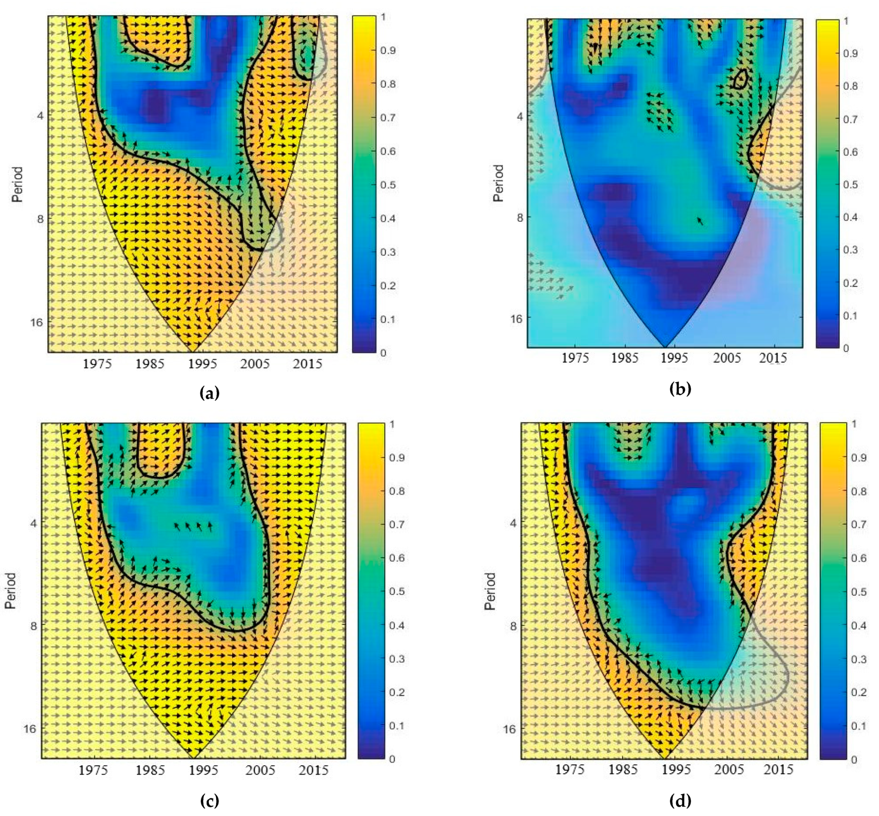
3.2.5. Wavelet Approach

The wavelet approach is utilized in the current research to gather information about the dependency of time-frequency between GDP, urbanization (URB), energy use (EU), CO2 emissions (CO2), and trade openness (TO) in Brazil. Goupillaud et al. [82] initiated the Morlet family. It is commonly accepted that when time series variables are estimated and they are not stationary, the result will yield bias estimates if the conventional time-domain method is not employed [83]. Additionally, in the field of economics and finance, time-series data are prone to break(s); hence conventional causality test outcomes with parameters fixed are susceptible to surface [26]. Contrary to time-domain causality, the standalone frequency domain method is a major concern, also known as Fourier transform. Therefore, to abolish the estimation issues, the wavelet coherence technique is utilized. Morlet wavelet equation is presented below:
ϖ ( t ) π 1 4 e i ϖ t e 1 2 t 2 ,
where: utilizing 𝓌 . on the limited frequency of the time series; i is 1 ; 0, 1, 2, …, N−1 represent p( t ), 𝓃 . Transmuting the time series into the domaintime-frequency and converts into the wavelet changes. In Equation (15), the ϖ is altered as ϖ k ,   f .
ϖ k ,   f ( t ) = 1 h ϖ ( t k f ) ,       k , f ,   f 0 ,
where: frequency and time was defined as f and t respectively. Adebayo and Odugbesan [7] assert that the major parameters of any wavelet approach are f and t . The Equation (17) explains CWT as:
ϖ p ( k ,   f ) = p ( t ) 1 f ϖ ( t k ¯ f ) i d s .
In Equation (17), p(t), which denotes the time series is transform along with 𝓌 .
p ( t ) = 1 C ϖ 0 [ | w p ( a ,   b ) | 2 d a ] d b b 2 .
The times series’ vulnerability can be captured by employing the wavelets power spectrum, which is denoted in Equation (18)
W P S p ( k , f   ) = | W P ( k ,   f ) | 2 .
Furthermore, Equation for the cross wavelets transform (CWT) for two times series is explained as:
W p q ( k ,   f ) = W p ( k , f ) W q ( k ,   f ) ¯   ,
where: W q ( k ,   f ) and W p ( k ,   f ) are the times series of CWT, respectively. Equation (21) gives a clear definition of the wavelet coherence square.
R 2 ( k ,   f ) = | S ( f 1 W p q ( k ,   f ) ) | 2 S ( f 1 | W p ( k ,   f ) | 2 ) S ( f 1 | W q ( k ,   f ) | 2 ) .
The R 2 ( k ,   f ) indicatesthe strength of the association, not considering the recommended nature of this interaction. Phase difference was initiated by Torrence and Compo [84] to indicate the direction of the connection through wavering the time series and is defined in Equation (21).
ϕ p q ( k ,   f ) = tan 1 ( L { S ( f 1 W p j ( k ,   f ) ) } O { S ( f 1 W p j ( k ,   f ) ) } ) ,
where: The real component and imaginary operator are denoted as O and L, respectively.

3.2.6. Gradual Shift Causality

The model developed by Toda and Yamamoto [85], which depends on vector autoregressive (VAR) built by Sims [86]. In calculating for the optimal lag length, p + dmax is added to the lag of dmax (the maximal integrated order of the time series). However, the VAR model outcome can be unreliable since structural shifts are ignored [87,88]. For this reason, to scrutinize the causal association between CO2, GDP, REN, GLO, and FD, this study utilized the Fourier Toda-Yamamoto causality test, an innovation of Nazlioglu et al. [89] to capture the structural shifts in Granger causality analysis and including the gradual and smooth shift. It can also be called the “gradual-shift causality test”. Nazlioglu et al. [89] initiated the Fourier Granger causality test with a single frequency (SF) and cumulative frequencies (CF) respectively, known as Fourier approximation. By adding the TY-VAR analysis and Fourier approximation, the modified Wald test statistic (MWALT) is generated. Assuming the coefficients of the intercept is constant over time, which modifies the VAR model into Equation (23) as follows:
y t =   σ ( t ) +   β 1 y t 1 + + β p + d m a x y t ( p + d m a x ) + ε t ,
where y t denotes CO2, GDP, EC, URB, and TO; σ, β, ε, and t denote intercept, coefficient matrices, error term, and time function correspondingly. To capture the structural change, the following Fourier expansion is introduced and explained as in Equation (24).
σ ( t ) = σ 0 + k = 1 n γ 1 k sin ( 2 π k t T ) + k = 1 n γ 2 k cos ( 2 π k t T ) ,  
where the frequency amplitude and displacement was measured by γ 1 k and γ 2 k correspondingly, and n denotes the number of frequency.
Substituting Equation (24) into Equation (23), the structural shift are thereby put into consideration, defines the Fourier Toda-Yamamoto causality with cumulative frequencies (CF), as follows in Equation (25).
y t = σ 0 + k = 1 n γ 1 k sin ( 2 π k t T ) + k = 1 n γ 2 k cos ( 2 π k t T ) + β 1 y t 1 + + β p + d m a x y t ( p + d m a x ) + ε t
Wherek denoted approximation frequency. The components in single frequency are illustrated in Equation (26) as:
σ ( t ) = σ 0 + γ 1 sin ( 2 π k t T ) + γ 2 cos ( 2 π k t T ) .
Equation (24) into Equation (25) was substituted, which defines the Fourier Toda-Yamamoto causality with single frequencies in Equation (27) as:
y t = σ 0 + γ 1 sin ( 2 π k t T ) + γ 2 cos ( 2 π k t T ) + β 1 y t 1 + + β p + d y t ( p + d ) + ε t
Here, the testing of the null hypothesis of non-causality is zero (H0: β1 = βθ = 0), and the Wald statistic can be used for testing the hypothesis.

4. Findings and Discussion

The present research tends to close this gap in the literature by exploring CO2 emissions (CO2) and real growth (GDP) in Brazil, while also accounting for the role of urbanization (URB), trade openness (TR), and energy usage (EC) utilizing data stretching between 1965 and 2019. Accordingly, the simple summary statistical features illustrated in Table 3 display the central tendencies measure and dispersion indicate that urbanization has the highest average, accompanied by energy usage, real growth, and CO2 emissions and trade openness. The outcomes of skewness illustrates that all the variables of interest affirm to normal distribution. Furthermore, the kurtosis outcomes outline that only TR and URB comply with normal distribution. TO and URB do not conform to normal distribution. Furthermore, the study utilized the Zivot and Andrews [70] test to ascertain the data stationarity characteristics, and the outcomes reveal that the series are integrated at I(0) and I(1)as shown in Table 4. Prior to estimating the relationship between series, it is essential to examine the long-run association among the parameters. Based on this, the current study utilized Maki [73] cointegration which can capture both cointegration and five breaks in series respectively. The study also utilized the conventional bounds test as a robustness check to the Maki cointegration test. The outcomes of the Maki [73] and bounds tests are depicted in Table 5 and Table 6, respectively, and the outcomes revealed evidence of cointegration among the series.
The long and short-run connection between the series of interest was estimated, with the results shown in Table 7. This research proceeds to explore the magnitude of the long-run relationship established. Batteries of analyses were applied for the soundness of coefficients and estimations. Table 8 outlined the FMOLS and DOLS, with the dependent variable as GDP growth while CO2, TO, URB, and EC as explanatory variables. We observe that energy consumption enhances economic growth as we observe that a 1% increase in energy consumption increases economic growth by a magnitude of 0.46%, and 0.47% by FMOLS and DOLS estimators correspondingly. This result lends credence to the energy-induced growth hypothesis that is supported by Ali et al. [53], Awosusi et al. [30], Udemba et al. [64], and Shahbaz et al. [90]. This result implies that the Brazilian economy is energy-driven and that energy-conservation policies will jeopardize economic expansion. Moreover, both regression estimators show that urbanization affects GDP growth in Brazil, which is consistent with an optimistic association between GDP growth and urbanization. According to FMOLS and DOLS outcomes, a 1% rise in urbanization raises GDP by 1.10% and 1%, accordingly. Authors prove the argument centered on empirical evidence that Brazil’s population increase is advantageous to the country’s economic path. That being said, policymakers must exercise vigilance in matching urban facilities and services in rural areas. This is to stop a drive to metropolitan cities, since most government leaders prefer urban development over rural development. Otherwise, urban infrastructure could become overburdened, stifling long-term economic growth. Additionally, government officials need to encourage public–private partnerships (PPP) in terms of building infrastructure in other less urbanized regions to balance the infrastructural deficit in both rural and urban areas. This alludes to the fact that small and medium enterprises (SME) are a key driver of any economy which will have a ripple effect on the pace of other macroeconomic indicators and economic development at large. This outcome complies with the study of Awosusi et al. [30], Adebayo, [91], Ali et al. [53], and Nathaniel and Bekun [6], who established that urbanization enhances economic performance.
Furthermore, there is proof of a long-run connection between GDP and CO2 emissions, with FMOLS and DOLS showing that a 0.24% and 0.26% rise in GDP is related to a 1% upsurge in CO2, accordingly. This is unsurprising considering that the economy of Brazilian is predominantly an industrial and investment-based economy that strongly depends on the usage of energy. Nevertheless, one optimistic outcome of this is the ability to mitigate CO2 pollution by changing the energy mix to incorporate more renewable options, including solar and wind energy (renewables). This outcome is consistent with the studies of Rjoub et al. [1] for Turkey, Kirikkaleli and Adebayo [8] for India, Udemba et al. [65] for India, and Awosusi et al. [30] for South Korea. On the connection between trade openness and GDP, an insignificant relationship was observed. Thus, suggesting that trade in Brazil has an insignificant effect on GDP suggests that openness of the Brazilian economy to the outside world does not promote economic progress. This study aligns with the findings of Hossain [92] for Japan, Udemba et al. [64] for Indonesia, and Awosusi et al. [30] for South Korea who established an insignificant linkage between trade openness and economic growth. Thus, policymakers need to insulate the economy against detrimental economic impact. This further explains the nature of the trade pattern between Brazil and the rest of the world due to Brazil’s economic structure and size. The goodness of fit of the model is presented by the R2 (0.98) and AdjR2(0.97) accordingly.
The correlation and causality between CO2 and its determinants in Brazil are captured simultaneously at different frequencies (low, medium, and high) by utilizing the wavelet coherency. The right-hand side of Figures has a color bar which depicts the frequencies in term of strength of correlation, moving from yellow (high frequency) to blue (low frequency). At the left-side of Figures, the period (scale) can be classified into the long, medium, and short period, which is 8–16, 4–8, and 0–4, respectively. Furthermore, the arrows in the rightward direction depict a positive correlation while the negative correlation is depicted by arrows in the leftward direction. Finally, when the direction of the arrow is rightward (up) and leftward (down), it means the second variable is leading the first variable and also when the movement of the arrow is rightward (down) and leftward (up), it indicates that the first variable is leading the second variable. The blue and yellow colors depict low and high dependence between the series. The WTC between CO2 and GDP is presented in Figure 3a. At medium and low frequencies between 1965 and 2019, the series are in-phase which mirrors positive comovement between CO2 and GDP. Figure 3b depicts the WTC between trade openness and GDP between 1965 and 2019. At different frequencies between 1965 and 2003, there is no proof of a significant comovement between trade openness and GDP, though there is evidence of in-phase connection between trade openness and GDP between 2008 and 2015 at middle frequency. Figure 3c portrays the WTC between energy usage and GDP between 1965 and 2019. At different frequencies, between 1970 and 2017, there is in-phase (positive correlation) between energy usage and GDP mostly in the medium and short frequencies. Figure 3d portrays the WTC between urbanization and GDP between 1965 and 2019. At different frequencies between 1970 and 1985 and between 2005 and 2016, there is positive comovement between urbanization and GDP. The outcomes from the wavelet coherence test are consistent with outcomes of the ARDL, FMOLS, and DOLS.
The study employed the Gradual shift causality test to capture the causal impacts of CO2, EN, URB, and TR on GDP in capturing the causal interaction between series even in the existence of structural break, which is the novelty of the Gradual shift causality. In Table 7, the causality analysis is reported. The Causality results confirm that energy consumption causes GDP in Brazil, thus validating that energy usage is a key contributing factor of GDP. This result resonates with the outcomes of Ali et al. [53] for the case of Nigeria and Shahbaz et al. [90] in Pakistan. Additionally, authors also observe that urbanization and trade openness Granger causes economic growth. These results confirm the finding of Udemba et al. [64] and Ali et al. [53], i.e., urbanization and openness are better predictors to explain economic growth in Brazil over our study period. This finding has consequences for Brazil’s economic growth concerning rapid urbanization, where investment will be harnessed mainly to the vulnerable population with the promise of improvement in welfare. Additionally, there is an indication of unidirectional causality from CO2 to GDP which infers that CO2 is a strong predictor of GDP in Brazil. In this regard, Brazilian policymakers should build policies in line with the nation’s energy portfolio diversification. This outcome complies with the study of Adebayo [92] for Mexico, and Zhang et al. [36] for Malaysia.

5. Conclusions

The global concern for protecting the environment is reflected in a wide range of policy mandate, and development policies concentrate greatly on whether sustainable growth could lead to environmental degradation. This study is distinct from those previously documented in the extant literature in terms of the scope for Brazil, where few entries have been recorded. Furthermore, the research utilized econometrics strategies, namely, DOLS, FMOLS, Maki Cointegration, ARDL bounds, and the robust Wavelet and Gradual-shift causality to capture the connections between these economic indicators. The outcomes of both Maki cointegration and ARDL bounds testing to cointegration affirm the presence of long-run interaction among the parameters of interest, indicating the convergence of the explanatory variables and explaining their growth association. The outcomes from FMOLS and DOLS validate the energy-induced hypothesis. This is very insightful for government officials in Brazil; that is, energy is a key determinant to stimulate sustainable economic growth. The positive impact of urbanization and economic growth is insightful in Brazil, and this suggests that the urban growing population is productive as urbanization is seen to stimulate economic growth. This further implies that the population is productive which is desirable given that Brazil is still an emerging economy is a novel revelation. Nevertheless, caution should be placed to circumvent drift in rural-urban that might put pressure on the urban cities, which might harm economic growth in Brazil. Moreover, the urban-economic growth connection is also validated by the causality analysis where uni-directional causality is found running from urbanization to economic growth. This suggests that urbanization is a good predictor of economic growth in Brazil. Furthermore, the association between economic growth and trade openness is insignificant. The plausible explanation could be that the trade openness is not favorable to the fragile developing economy which should be insulated from such threats to economic progress, especially the infant industries.
Based on the outcomes above, the Brazilian government must preserve its energy sector, as energy is a predictor of GDP growth. Nonetheless, there is concern on the part of the government if external shock hits the energy sector or the country cannot deal with energy cuts and might need to diversify the economy into other growth paths to ameliorate against any unforeseen circumstance. Additionally, the country cannot embark on energy-conservative strategies because such acts will jeopardize economic progress. Furthermore, the statistical relationship between urbanization and economic growth is an indicator for decision-makers. This is a call to sustain such a milestone as it shows the urban population contributes to economic progress. However, caution is needed to strike a balance between rural and urban dwellers to avoid drift to urban cities and overpressure on urban infrastructures, thereby serving as a threat to economic growth which could, in turn, affect the sustainable development of the country. Renewable sources, including hydropower, ocean power, geothermal, wind power, and solar, should be considered cleaner and substitutes to utilize nonrenewable energy in economic activities. In summary, as a nation, Brazil has more prospects to preserve sustainable growth in both environmental and economic operations. The outcomes of this research would impact neighboring nations positively if they were willing to take the steps proposed in this research to reinforce their sustainable growth. Overwhelmingly, this study has examined the linkage between economic performance and environmental sustainability by taking into account the role of energy consumption, urbanization and trade openness in Brazil using data spanning between 1965 and 2019. Nonetheless, more research should be done for other developing economies, taking into account asymmetric econometrics modeling or the usage of micro disaggregated data. Moreover, other research may also take into consideration other drivers of growth not examined in this research.

Author Contributions

T.S.A. designed the experiment and collect the dataset. The introduction and literature review sections are written by A.A.A. and G.D.A. and T.S.A., W.-K.W. and J.A.O. constructed the methodology section and empirical outcomes in the study. T.S.A. and H.R. contributed to the interpretation of the outcomes. All authors have read and agreed to the published version of the manuscript.

Funding

The fifth author would like to thank Robert B. Miller and Howard E. Thompson for their continuous guidance and encouragement. This research has been supported by Asia University, China Medical University Hospital, The Hang Seng University of Hong Kong, Research Grants Council (RGC) of Hong Kong (project number 12500915), and Ministry of Science and Technology (MOST, Project Numbers 106-2410-H-468-002 and 107-2410-H-468-002-MY3), Taiwan.

Institutional Review Board Statement

Not applicable.

Informed Consent Statement

Not applicable.

Data Availability Statement

The data that support the findings of this study are available from World Bank.

Conflicts of Interest

The author declares no competing interests.
Acronyms
ADFAugmented Dickey-Fuller
ARDLAutoregressive Distributed Lag
BRICSBrazil, Russia, India, China, and South Africa
CO2Carbon Dioxide
COP21UN Climate Change Conference in Paris
DOLSDynamic Ordinary Least Square
EKCEnvironmental Kuznets Curve
ENEnergy Consumption
FMOLSFully Modified Ordinary Least Squares
GDPEconomic Growth
GHGsGreenhouse Gas Emissions
GMMGeneralized Method of Moments
IEAInternational Energy Agency
OECDThe Organization for Economic Co-operation and Development
PMG-ARDLPooled Mean Group Autoregressive Distributed Lag
PPPhillips-Perron
R&DResearch and Development
TYToda and Yamamoto
UAEUnited Arab Emirates
VARVector Autoregression
ZAZivot and Andrews
Symbols
θ Coefficient of the Regressors
ρ Speed of adjustment
e t Error term
H 0 Null hypothesis
H a Alternative hypothesis

References

  1. Rjoub, H.; Odugbesan, J.A.; Adebayo, T.S.; Wong, W.K. Sustainability of the Moderating Role of Financial Development in the Determinants of Environmental Degradation: Evidence from Turkey. Sustainability 2021, 13, 1844. [Google Scholar] [CrossRef]
  2. Adebayo, T.S.; Kirikkaleli, D. Impact of renewable energy consumption, globalization, and technological innovation on environmental degradation in Japan: Application of wavelet tools. Environ. Dev. Sustain. 2021, 1–26. [Google Scholar] [CrossRef]
  3. Cioca, L.I.; Ivascu, L.; Rada, E.C.; Torretta, V.; Ionescu, G. Sustainable development and technological impact on CO2 reducing conditions in Romania. Sustainability 2015, 7, 1637–1650. [Google Scholar] [CrossRef] [Green Version]
  4. Stern, N.H.; Peters, S.; Bakhshi, V.; Bowen, A.; Cameron, C.; Catovsky, S.; Zenghelis, D. Stern Review: The Economics of Climate Change; Cambridge University Press: Cambridge, UK, 2006; Volume 30, p. 2006. [Google Scholar]
  5. EIA U Energy Information Administration. International Energy Outlook. US Department of Energy. Available online: https://www.iea.org/countries/brazil (accessed on 1 March 2021).
  6. Nathaniel, S.P.; Bekun, F.V. Electricity consumption, urbanization, and economic growth in Nigeria: New insights from combined cointegration amidst structural breaks. J. Public Aff. 2021, 21, e2102. [Google Scholar] [CrossRef] [Green Version]
  7. Adebayo, T.S.; Odugbesan, J.A. Modeling CO2 emissions in South Africa: Empirical evidence from ARDL based bounds and wavelet coherence techniques. Environ. Sci. Pollut. Res. 2020, 28, 9377–9389. [Google Scholar] [CrossRef] [PubMed]
  8. Kirikkaleli, D.; Adebayo, T.S. Do public-private partnerships in energy and renewable energy consumption matter for consumption-based carbon dioxide emissions in India? Environ. Sci. Pollut. Res. 2021, 1–14. [Google Scholar] [CrossRef]
  9. Odugbesan, J.A.; Rjoub, H. Relationship among Economic Growth, Energy Consumption, CO2 Emission, and Urbanization: Evidence from MINT Countries. SAGE Open 2020, 10, 2158244020914648. [Google Scholar] [CrossRef] [Green Version]
  10. World Bank World Development Indicators. Available online: http://data.worldbank.org/ (accessed on 1 March 2021).
  11. Carbonbrief. Available online: https://www.carbonbrief.org/the-carbon-brief-profile-brazil (accessed on 1 March 2021).
  12. BP. British Petroleum. Available online: https://www.bp.com/en/global/corporate/energy-economics/statistical-review-of-world-energy.html (accessed on 1 March 2021).
  13. Dias, J. Climate Politics: Contemporary Trend to Achieve Energy Security and Environment Sustainability–Case Studies of INDIA and BRAZIL (1972 to 2018). East. Afr. J. 2019, 2, 22–31. [Google Scholar]
  14. Malefane, M.R.; Odhiambo, N.M. Trade Openness and Economic Growth: Empirical Evidence from Lesotho. Glob. Bus. Rev. 2019. [Google Scholar] [CrossRef]
  15. Iyoha, M.; Okim, A. The impact of trade on economic growth in ECOWAS countries: Evidence from panel data. CBNJ Appl. Stat. 2017, 8, 23–49. [Google Scholar]
  16. Adhikary, B.K. FDI, Trade Openness, Capital Formation, and Economic Growth in Bangladesh: A Linkage Analysis. Int. J. Bus. Manag. 2010, 6, 16. [Google Scholar] [CrossRef]
  17. Buhari, D.Ğ.A.; Lorente, D.B.; Nasir, M.A. European commitment to COP21 and the role of energy consumption, FDI, trade and economic complexity in sustaining economic growth. J. Environ. Manag. 2020, 273, 111146. [Google Scholar]
  18. Abbott, J. Green Infrastructure for Sustainable Urban.Development in Africa; Routledge: London, UK, 2013. [Google Scholar]
  19. Bouznit, M.; Pablo-Romero, M.D.P. CO2 emission and economic growth in Algeria. Energy Policy 2016, 96, 93–104. [Google Scholar] [CrossRef]
  20. Lacheheb, M.; Rahim, A.S.A.; Sirag, A. Economic growth and CO2 emissions: Investigating the environmental Kuznets curve hypothesis in Algeria. Int. J. Energy Econ. Policy 2015, 5, 4. [Google Scholar]
  21. Bastola, U.; Sapkota, P. Relationships among energy consumption, pollution emission, and economic growth in Nepal. Energy 2015, 80, 254–262. [Google Scholar] [CrossRef]
  22. Aye, G.C.; Edoja, P.E. Effect of economic growth on CO2 emission in developing countries: Evidence from a dynamic panel threshold model. Cogent Econ. Financ. 2017, 5, 1379239. [Google Scholar] [CrossRef]
  23. Gorus, M.S.; Aydin, M. The relationship between energy consumption, economic growth, and CO2 emission in MENA countries: Causality analysis in the frequency domain. Energy 2019, 168, 815–822. [Google Scholar] [CrossRef]
  24. Wang, S.; Li, Q.; Fang, C.; Zhou, C. The relationship between economic growth, energy consumption, and CO2 emissions: Empirical evidence from China. Sci. Total. Environ. 2016, 542, 360–371. [Google Scholar] [CrossRef]
  25. Muhammad, B. Energy consumption, CO2 emissions and economic growth in developed, emerging and Middle East and North Africa countries. Energy 2019, 179, 232–245. [Google Scholar] [CrossRef]
  26. Kirikkaleli, D.; Adebayo, T.S. Do renewable energy consumption and financial development matter for environmental sustainability? New global evidence. Sustain. Dev. 2020, 4, 23–36. [Google Scholar] [CrossRef]
  27. He, X.; Adebayo, T.S.; Kirikkaleli, D.; Umar, M. Analysis of Dual Adjustment Approach: Consumption-Based Carbon Emissions in Mexico. Sustain. Prod. Consum. 2021, 27, 947–957. [Google Scholar] [CrossRef]
  28. Khobai, H.; Le Roux, P. The relationship between energy consumption, economic growth and carbon dioxide emission: The case of South Africa. Int. J. Energy Econ. Policy 2017, 7, 102–109. [Google Scholar]
  29. Salahuddin, M.; Alam, K.; Ozturk, I.; Sohag, K. The effects of electricity consumption, economic growth, financial development and foreign direct investment on CO2 emissions in Kuwait. Renew. Sustain. Energy Rev. 2018, 81, 2002–2010. [Google Scholar] [CrossRef] [Green Version]
  30. Awosusi, A.A.; Adebayo, T.S.; Kirikkaleli, D.; Akinsola, G.D.; Mwamba, M.N. Can CO2 emissiovns and energy consumption determine the economic performance of South Korea? A time series analysis. Environ. Sci. Pollut. Res. 2021, 1–16. [Google Scholar] [CrossRef]
  31. Adebayo, T.S.; Kalmaz, D.B. Determinants of CO2 emissions: Empirical evidence from Egypt. Environ. Ecol. Stat. 2021, 1–24. [Google Scholar] [CrossRef]
  32. Acheampong, A.O. Economic growth, CO2 emissions and energy consumption: What causes what and where? Energy Econ. 2018, 74, 677–692. [Google Scholar] [CrossRef]
  33. Mikayilov, J.I.; Galeotti, M.; Hasanov, F.J. The impact of economic growth on CO2 emissions in Azerbaijan. J. Clean. Prod. 2018, 197, 1558–1572. [Google Scholar] [CrossRef]
  34. Saidi, K.; Hammami, S. The impact of CO2 emissions and economic growth on energy consumption in 58 countries. Energy Rep. 2015, 1, 62–70. [Google Scholar] [CrossRef] [Green Version]
  35. Begum, R.A.; Sohag, K.; Abdullah, S.M.S.; Jaafar, M. CO2 emissions, energy consumption, economic and population growth in Malaysia. Renew. Sustain. Energy Rev. 2015, 41, 594–601. [Google Scholar] [CrossRef]
  36. Zhang, L.; Li, Z.; Kirikkaleli, D.; Adebayo, T.S.; Adeshola, I.; Akinsola, G.D. Modelling CO2 emissions in Malaysia: An application of Maki cointegration and wavelet coherence tests. Environ. Sci. Pollut. Res. 2021, 1–15. [Google Scholar] [CrossRef]
  37. Adedoyin, F.F.; Gumede, M.I.; Bekun, F.V.; Etokakpan, M.U.; Balsalobre-Lorente, D. Modelling coal rent, economic growth and CO2 emissions: Does regulatory quality matter in BRICS economies? Sci. Total Environ. 2020, 710, 136284. [Google Scholar] [CrossRef]
  38. Balsalobre-Lorente, D.; Shahbaz, M.; Roubaud, D.; Farhani, S. How economic growth, renewable electricity and natural resources contribute to CO2 emissions? Energy Policy 2018, 113, 356–367. [Google Scholar] [CrossRef] [Green Version]
  39. Chen, P.Y.; Chen, S.T.; Hsu, C.S.; Chen, C.C. Modelling the global relationships among economic growth, energy consumption and CO2 emissions. Renew. Sustain. Energy Rev. 2016, 65, 420–431. [Google Scholar] [CrossRef]
  40. Ahmad, N.; Du, L. Effects of energy production and CO2 emissions on economic growth in Iran: ARDL approach. Energy 2017, 123, 521–537. [Google Scholar] [CrossRef]
  41. Aslan, A.; OğuzÖCA, L.; Shahbaz, M. Energy Consumption–Trade Openness–Economic Growth Nexus in G-8 Countries. Kapadokya Akad. 2017, 1, 71–97. [Google Scholar]
  42. Gökmenoğlu, K.; Taspinar, N. The relationship between CO2 emissions, energy consumption, economic growth and FDI: The case of Turkey. J. Int. Trade Econ. Dev. 2015, 25, 706–723. [Google Scholar] [CrossRef]
  43. Gozgor, G.; Lau, C.K.M.; Lu, Z. Energy consumption and economic growth: New evidence from the OECD countries. Energy 2018, 153, 27–34. [Google Scholar] [CrossRef] [Green Version]
  44. Baz, K.; Xu, D.; Ampofo, G.M.K.; Ali, I.; Khan, I.; Cheng, J.; Ali, H. Energy consumption and economic growth nexus: New evidence from Pakistan using asymmetric analysis. Energy 2019, 189, 116254. [Google Scholar] [CrossRef]
  45. Le, H.P. The energy-growth nexus revisited: The role of financial development, institutions, government expenditure and trade openness. Heliyon 2020, 6, e04369. [Google Scholar] [CrossRef]
  46. Raghutla, C. The effect of trade openness on economic growth: Some empirical evidence from emerging market economies. J. Public Aff. 2020, 20, e2081. [Google Scholar] [CrossRef]
  47. Ahmed, K. Revisiting the role of financial development for energy-growth-trade nexus in BRICS economies. Energy 2017, 128, 487–495. [Google Scholar] [CrossRef]
  48. Kumari, D.; Malhotra, N. Export-led growth in India: Cointegration and causality analysis. J. Econ. Dev. Stud. 2014, 2, 297–310. [Google Scholar]
  49. Egoro, S.; Obah, O.D. The impact of international trade on economic growth in Nigeria: An econometric analysis. Asian Financ. Bank. Rev. 2017, 1, 28–47. [Google Scholar] [CrossRef]
  50. Coulibaly, R.G. International trade and economic growth: The role of institutional factors and ethnic diversity in sub-Saharan Africa. Int. J. Finance Econ. 2021. [Google Scholar] [CrossRef]
  51. Amna Intisar, R.; Yaseen, M.R.; Kousar, R.; Usman, M.; Makhdum, M.S.A. Impact of trade openness and human capital on economic growth: A comparative investigation of Asian countries. Sustainability 2020, 12, 2930. [Google Scholar] [CrossRef] [Green Version]
  52. Zheng, W.; Walsh, P.P. Economic growth, urbanization and energy consumption—A provincial level analysis of China. Energy Econ. 2019, 80, 153–162. [Google Scholar] [CrossRef]
  53. Ali, H.S.; Nathaniel, S.P.; Uzuner, G.; Bekun, F.V.; Sarkodie, S.A. Trivariatemodelling of the nexus between electricity consumption, urbanization and economic growth in Nigeria: Fresh insights from Maki Cointegration and causality tests. Heliyon 2020, 6, e03400. [Google Scholar] [CrossRef]
  54. Bakirtas, T.; Akpolat, A.G. The relationship between energy consumption, urbanization, and economic growth in new emerging-market countries. Energy 2018, 147, 110–121. [Google Scholar] [CrossRef]
  55. Nguyen, H.M. The relationship between urbanization and economic growth: An empirical study on ASEAN countries. Int. J. Soc. Econ. 2018, 45, 316–339. [Google Scholar] [CrossRef]
  56. Šatrović, E.; Dağ, M. Energy consumption, urbanization and economic growth relationship: An examination on OECD countries. Dicle Üniversitesi Sosyal Bilimler Enstitüsü Dergisi 2019, 11, 315–324. [Google Scholar]
  57. Liddle, B.; Messinis, G. Which comes first—Urbanization or economic growth? Evidence from heterogeneous panel causality tests. Appl. Econ. Lett. 2014, 22, 349–355. [Google Scholar] [CrossRef]
  58. Solarin, S.A.; Shahbaz, M.; Shahzad, S.J.H. Revisiting the electricity consumption-economic growth nexus in Angola: The role of exports, imports and urbanization. Int. J. Energy Econ. Policy 2016, 6, 501–512. [Google Scholar]
  59. Kuznets, S.; Murphy, J.T. Modern Economic Growth: Rate, Structure, and Spread; Yale University Press: New Haven, CT, USA, 1966; Volume 2. [Google Scholar]
  60. Panayotou, T. Empirical Tests and Policy Analysis of Environmental Degradation at Different Stages of Economic Development; International Labour Organization: Geneva, Switzerland, 1993; No. 992927783402676. [Google Scholar]
  61. Grossman, G.M.; Krueger, A.B. Environmental impacts of a North. In American Free Trade Agreement; (No. w3914); National Bureau of Economic Research: Cambridge, MA, USA, 1991; Available online: https://www.nber.org/system/files/working_papers/w3914/w3914.pdf (accessed on 24 January 2021).
  62. Shafik, N.; Bandyopadhyay, S. Economic Growth and Environmental Quality: Time-Series and Cross-Country Evidence; World Bank Publications: Berlin, Germany, 1992; Volume 904. [Google Scholar]
  63. Bekun, F.V.; Agboola, M.O.; Joshua, U. Fresh Insight into the EKC Hypothesis in Nigeria: Accounting for Total Natural. In Econometrics of Green Energy Handbook: Economic and Technological Development; Springer: Berlin, Germany, 2020; p. 221. [Google Scholar]
  64. Udemba, E.N.; Güngör, H.; Bekun, F.V.; Kirikkaleli, D. Economic performance of India amidst high CO2 emissions. Sustain. Prod. Consum. 2021, 27, 52–60. [Google Scholar] [CrossRef]
  65. Udemba, E.N.; Magazzino, C.; Bekun, F.V. Modeling the nexus between pollutant emission, energy consumption, foreign direct investment, and economic growth: New insights from China. Environ. Sci. Pollut. Res. 2020, 27, 17831–17842. [Google Scholar] [CrossRef]
  66. Bekun, F.V.; Agboola, M.O. Electricity Consumption and Economic Growth Nexus: Evidence from Maki Cointegration. Eng. Econ. 2019, 30, 14–23. [Google Scholar] [CrossRef] [Green Version]
  67. Alam, M.J.; Begum, I.A.; Buysse, J.; Van Huylenbroeck, G. Energy consumption, carbon emissions and economic growth nexus in Bangladesh: Cointegration and dynamic causality analysis. Energy Policy 2012, 45, 217–225. [Google Scholar] [CrossRef]
  68. Alam, K.J.; Sumon, K.K. Causal relationship between trade openness and economic growth: A panel data analysis of asian countries. Int. J. Econ. Financ. Issues 2020, 10, 118–126. [Google Scholar] [CrossRef] [Green Version]
  69. Kong, Q.; Peng, D.; Ni, Y.; Jiang, X.; Wang, Z. Trade openness and economic growth quality of China: Empirical analysis using ARDL model. Finance Res. Lett. 2021, 38, 101488. [Google Scholar] [CrossRef]
  70. Zivot, E.; Andrews, D.W.K. Further Evidence on the Great Crash, the Oil-Price Shock, and the Unit-Root Hypothesis. J. Bus. Econ. Stat. 2002, 20, 25–44. [Google Scholar] [CrossRef]
  71. Hatemi, J.A. Tests for cointegration with two unknown regime shifts with an application to financial market integration. Empir. Econ. 2008, 35, 497–505. [Google Scholar] [CrossRef]
  72. Gregory, A.W.; Hansen, B.E. Residual-based tests for cointegration in models with regime shifts. J. Econ. 1996, 70, 99–126. [Google Scholar] [CrossRef] [Green Version]
  73. Maki, D. Tests for cointegration allowing for an unknown number of breaks. Econ. Model. 2012, 29, 2011–2015. [Google Scholar] [CrossRef]
  74. Odugbesan, J.A.; Rjoub, H. Evaluating HIV/Aids prevalence and sustainable development in sub-Saharan Africa: The role of health expenditure. Afr. Health Sci. 2020, 20, 568–578. [Google Scholar] [CrossRef]
  75. Odugbesan, J.A. The causal relationship between economic growth and remittance in mint countries: An ardl bounds testing approach to cointegration. J. Acad. Res. Econ. 2019, 11, 310–329. [Google Scholar]
  76. Narayan, P.K. Fiji’s tourism demand: The ARDLapproach to cointegration. Tour. Econ. 2004, 10, 193–206. [Google Scholar] [CrossRef]
  77. Ayobamiji, A.A.; Kalmaz, D.B. Reinvestigating the determinants of environmental degradation in Nigeria. Int. J. Econ. Policy Emerg. Econ. 2020, 13, 52–71. [Google Scholar] [CrossRef]
  78. Pesaran, M.H.; Timmermann, A. Small sample properties of forecasts from autoregressive models under structural breaks. J. Econ. 2005, 129, 183–217. [Google Scholar] [CrossRef] [Green Version]
  79. Narayan, P.K.; Narayan, S. Estimating income and price elasticities of imports for Fiji in a cointegration framework. Econ. Model. 2005, 22, 423–438. [Google Scholar] [CrossRef]
  80. Phillips, P.C.B.; Hansen, B.E. Statistical Inference in Instrumental Variables Regression with I(1) Processes. Rev. Econ. Stud. 1990, 57, 99–125. [Google Scholar] [CrossRef]
  81. Stock, J.H.; Watson, M.W. A Simple Estimator of Cointegrating Vectors in Higher Order Integrated Systems. Econometrica 1993, 61, 783. [Google Scholar] [CrossRef]
  82. Goupillaud, P.; Grossmann, A.; Morlet, J. Cycle-octave and related transforms in seismic signal analysis. Geoexploration 1984, 23, 85–102. [Google Scholar] [CrossRef]
  83. Adebayo, T.S.; Akinsola, G.D.; Odugbesan, J.A.; Olanrewaju, V.O. Determinants of Environmental Degradation in Thailand: Empirical Evidence from ARDL and Wavelet Coherence Approaches. Pollution 2021, 7, 181–196. [Google Scholar]
  84. Torrence, C.; Compo, G.P. A practical guide to wavelet analysis. Bull. Am. Meteorol. Soc. 1998, 79, 61–78. [Google Scholar] [CrossRef] [Green Version]
  85. Toda, H.Y.; Yamamoto, T. Statistical inference in vector autoregressions with possibly integrated processes. J. Econ. 1995, 66, 225–250. [Google Scholar] [CrossRef]
  86. Sims, C.A. Macroeconomics and reality. Econometrica 1980, 48, 1–48. [Google Scholar] [CrossRef] [Green Version]
  87. Enders, W.; Lee, J. A Unit Root Test Using a Fourier Series to Approximate Smooth Break. Oxf. Bull. Econ. Stat. 2011, 74, 574–599. [Google Scholar] [CrossRef] [Green Version]
  88. Enders, W.; Jones, P. Grain prices, oil prices, and multiple smooth breaks in a VAR. Stud. Nonlinear Dyn. Econ. 2016, 20, 399–419. [Google Scholar] [CrossRef]
  89. Nazlioglu, S.; Gormus, N.A.; Soytas, U. Oil prices and real estate investment trusts (REITs): Gradual-shift causality and volatility transmission analysis. Energy Econ. 2016, 60, 168–175. [Google Scholar] [CrossRef]
  90. Shahbaz, M.; Lean, H.H.; Shabbir, M.S. Environmental Kuznets Curve hypothesis in Pakistan: Cointegration and Granger causality. Renew. Sustain. Energy Rev. 2012, 16, 2947–2953. [Google Scholar] [CrossRef] [Green Version]
  91. Adebayo, T.S. Revisiting the EKC hypothesis in an emerging market: An application of ARDL-based bounds and wavelet coherence approaches. SN Appl. Sci. 2020, 2, 1–15. [Google Scholar] [CrossRef]
  92. Hossain, S. An Econometric Analysis for CO2 Emissions, Energy Consumption, Economic Growth, Foreign Trade and Urbanization of Japan. Low Carbon Econ. 2012, 3, 92–105. [Google Scholar] [CrossRef] [Green Version]
Figure 1. Share of energy mix by Source.
Sustainability 13 04371 g001
Figure 2. Flow of Analysis.
Sustainability 13 04371 g002
Figure 3. (a) Wavelet Coherence between Economic Growth and CO2 Emissions. (b) Wavelet Coherence between Economic Growth and Trade Openness. (c) Wavelet Coherence between Economic Growth and Energy Consumption. (d) Wavelet Coherence between Economic Growth and Urbanization.
Sustainability 13 04371 g003
Table 1. Synopsis of Studies.
Investigator (s)TimeframeNation (s)Technique(s)Outcomes
GDP, CO2, and EC
Acheampong [32]1990–2014116 nationsPVAR and GMMCO2 → GDP (−)
Adebayo and Odugbesan (2020)1971–2016South AfricaARDL and WCCO2 → GDP (+)
Adebayo et al. [7]1980–2018MINT economiesPARDL and Panel Granger causalityCO2 ≠ GDP
Adedoyin et al. [37]1990–2014BRICSPARDLCO2 → GDP (+)
Ahmad and Du [40]1971–2011IranARDLCO2 → GDP (+)
EC → GDP (+)
Aye andEdoja [22]1971–201331 developing economies.DPTMCO2 → GDP (−)
BastolaandSapkota [21]1980–2011NepalARDLCO2 → GDP (+)
Begum et al. [35]1980–2009MalaysiaMultivariate approachCO2 → GDP (+)
Bouznitand Pablo-Romero [19]1970–2010AlgeriaARDLCO2 → GDP (+)
EC → GDP
Baz et al. [44]1971–2014PakistanNARDLEC → GDP (+)
Chen et al. [39]1993–2010188 countriesVECMEC → GDP (−)
GökmenoğluandTaspinar [42]1974–2010TurkeyT-YCO2 → GDP
GorusandAydin [23])1975–20148 oil-rich MENAPanel causalityCO2 ≠ GDP
Gozgor et al. [43]1990–2013OECD countriesPARDLEC → GDP (+)
Khobaiand Le Roux [28]1971–2013South AfricaVECMCO2 → GDP (+)
EC ↔ GDP
Lacheheb et al. (2015)1971–2009AlgeriaARDLCO2 → GDP (+)
Le [20]1990–201446 developing nationsPanel causalityEC ↔ GDP
Mikayilov et al. [33]1992–2013AzerbaijanMultivariate approachCO2 → GDP (+)
Muhammad [25]2001–2017MENAGMMEC → GDP (−)
CO2 → GDP (+)
SaidiandHammami [34]1990–201258 countriesGMMCO2 → GDP (+)
Salahuddin et al. [29]1980–2013KuwaitARDL and VECMGDP → CO2
Wang et al. [24]1990–2017ChinaVECMCO2 ≠ GDP
Zhang et al. [36]1960–2018MalaysiaMC, T-Y, and Fourier T-YGDP → CO2
GDP and Trade Openness
Adhikary [15]1986–2008BangladeshVECMTR → GDP (−)
Ahmed [47]1991–2013BRICSPanel VECM Granger causalityGDP → TR
Coulibaly [50]1980–201744 sub-Saharan AfricaPARDLTR → GDP (+)
EgoroandObah [49]1981–2015NigeriaOLSTR → GDP (+)
IyohaandOkim [16]1990–2013ECOWASPOLS, fixed and Random effect modelTR → GDP (+)
KumariandMalhotra [48]1980–2012IndiaGranger causalityTR ↔GDP (+)
MalefaneandOdhiambo [14]1979–2013LesothoARDLTR ≠ GDP
Raghutla [46]1993–2016Emerging economiesPanel Granger causalityGDP → TR
GDP and Urban
Ali et al. [53]1971–2014NigeriaFMOLS, CCR and VECM causalityURB → GDP (−)
Nathaniel andBekun [6]1971–2014NigeriaFMOLS, DOLS, CCR and VECM causalityURB↔GDP (−)
Nguyen [55]1971–2014ASEANPMG and D-GMMURB → GDP(+)
Zhengand Walsh [52]2001–201229 provinces in ChinaFE and GMMURB → GDP (+)
ŠatrovićandDağ [56]1996–201534 OECDPVARURB → GDP (+)
Table 2. Variables Units and Sources.
VariableDescriptionUnitsSources
CO2Environmental SustainabilityMetric Tonnes Per CapitaBritish Petroleum
EC Energy ConsumedEnergy consumption per capita (kWh)
GDP Economic GrowthGDP Per Capita Constant $US, 2010World Development Indicators
TR Trade OpennessTrade % of GDP
URBUrbanizationUrban Population
Table 3. Descriptive Statistics.
GDPCO2ENTRURB
Mean3.9027830.1929203.9950301.2884348.022385
Median3.9216600.1866354.0207991.2862978.065876
Maximum4.0789450.4201694.2301801.4724388.263024
Minimum3.567361−0.1697613.5092011.0621287.628913
Std. Dev.0.1315630.1362540.1943130.1126080.191576
Skewness−1.041734−0.680209−1.008270−0.026551−0.516989
Kurtosis3.6358683.3044263.2533161.8364781.999171
Jarque-Bera10.874334.4536549.4659713.1088834.745509
Probability0.0043520.1078700.0088000.2113070.093224
Obs5555555555
Table 4. Zivot and Andrews Unit root Test.
At Level I(0)First Difference I(1)
I and TBreak−TimeI and TBreak−Time
GDP−6.352 ***2008−5.654 **2004
CO2−4.2502005−6.512 *2011
EC−6.744 *1997−7.604 *2003
TO−4.5432001−6.261 *2000
URB−4.1362010−6.326 *2010
Note: *, **, and *** stand for 1%, 5%, and 10% level of significance. I and T stand for intercept and trend.
Table 5. Maki Test.
Table 5. Maki Test.
T−StatisticsCritical Values
Model 5%Break−Years
Trend and Regime shifts
GDP = f(CO2, EC, URB, TO)−7.0670 *−6.9111997
GDP = f(CO2, EC, URB, TO)−8.67253 *−7.6381997, 1978
GDP = f(CO2, EC, URB, TO)−8.67253 *−8.2541997, 1978, 1989
GDP = f(CO2, EC, URB, TO)−11.8168 *−8.8711997, 1978, 1989, 2008
GDP = f(CO2, EC, URB, TO)−11.81687 *−9.4821997, 1978, 1989, 2008, 1971
Note: 5% significance level is signified by *.
Table 6. ARDLbounds Test.
Model EstimatedLag LengthF-StatisticsCointegration
GDP = f(CO2, EC, URB, TO)(2, 2, 0, 2, 0)6.59 *Yes
Significant LevelL-B I(0)U-B I(1)
0.053.254.49
0.13.745.06
Note: 1% level of significance denoted as *. L-B denotes the lower bounds while U-B denotes the upper bound. ARDL denotes autoregressive distributed lag.
Table 7. FMOLS and DOLS Outcomes.
FMOLSDOLS
VariablesCoefficientt-StatisticProbabilityCoefficientt-StatisticProbability
EN0.4610 *4.58400.0000.4798 *3.70960.000
CO20.2472 *3.61160.0000.2682 *2.99640.004
TR0.01350.67780.5010.01820.67720.501
URB1.1039 **1.77350.0831.0044 **2.41960.019
R20.980.98
Adj R20.970.97
S.E. of regression0.00860.009
Note: 1% level of significance denoted as *, 5% level of significance denoted as **. L-B denotes the lower bounds while U-B denotes the upper bound. FMOLS, DOLS denotes Fully Modified Ordinary Least Square and Dynamic ordinary least square.
Table 8. Gradual Shift Causality Outcomes
Causality PathWald-StatNo of Fourierp-ValueDecision
GDP → EN11.9172230.1033Do not Reject Ho
EN → GDP22.3597630.0022 *Reject Ho
GDP → URB3.88324120.7931Do not Reject Ho
URB → GDP14.1827420.0480 **Reject Ho
GDP → TR6.41887430.4917Do not Reject Ho
TR → GDP18.1892030.0111 **Reject Ho
CO2 → GDP21.4262530.0031 *Reject Ho
GDP → CO23.60095430.8244Do not Reject Ho
Note: Significance level of 1% and 5% is depicted by * and **.
Publisher’s Note: MDPI stays neutral with regard to jurisdictional claims in published maps and institutional affiliations.

