Spatiotemporal Distribution Characteristics and Influencing Factors Analysis of Reference Evapotranspiration in Beijing–Tianjin–Hebei Region from 1990 to 2019 under Climate Change

Abstract

Reference evapotranspiration (ET₀) is an important part of the water and energy cycles during crop growth. Understanding the influencing factors and spatiotemporal variations of ET₀ is of positive significance for guiding regional water-saving irrigation and regulating agricultural production. Data for daily meteorological observations of temperature, relative humidity, wind speed, and sunshine hours from 40 surface meteorological stations and the methods of climate tendency rate, Morlet wavelet, M-K mutation, path analysis, sensitivity analysis, and contribution rate analysis were utilized, to analyze the spatiotemporal distribution characteristics and influencing factors in the Beijing–Tianjin–Hebei region from 1990 to 2019. The ET₀ from 1990 to 2019 was 958.9 mm, and there was a significant downward trend in the climate tendency rate of −3.07 mm/10 a. The ET₀ presents a spatial distribution pattern decreasing from southwest to northeast. A change in the Beijing–Tianjin–Hebei region’s interannual ET₀ occurred in 2016, with a decrease of 41.12 mm since then. The ET₀ was positively correlated with temperature, wind speed, and sunshine hours, and negatively correlated with relative humidity; among those, wind speed and temperature are the dominant factors affecting the change of ET₀. This study provides a scientific basis for the regulation and control of agricultural production in the Beijing–Tianjin–Hebei region.

1. Introduction

Crop evapotranspiration refers to the process of leaf water transpiration and soil water evaporation, throughout the whole growth period of crops from sowing to maturity [1]. Reference evapotranspiration (ET₀) is an important indicator for characterizing atmospheric evapotranspiration as well as evaluating climate aridity, vegetation water consumption, production potential, and the balance of water supply and demand [2,3]. It is, also, a significant part of the water and energy cycles during crop growth [4]. The analysis of ET₀ is of significance, for understanding global climate evolution and improving the utilization of agricultural water resources [5].

The value of ET₀ is closely related to meteorological factors and crop conditions. Meteorological factors are the main influences on ET₀ change, and their influence will increase with global climate change [6,7,8]. The temporal and spatial variation characteristics of ET₀ and its influencing factors have become the focus of extensive attention of scholars, within and outside China. From the point of international research, Nam et al. [9] studied the impact of climate change on the change of reference evapotranspiration in Korea during 1973–1992, finding that temperature was the dominant factor. Liu et al. [10] found that the evapotranspiration in the Gulf of Mexico was affected by climate change, with spatial and temporal differences, from 1901 to 2008, and quantitative analysis showed that it had been, especially, affected by precipitation. Prăvălie et al. [11] studied the response of spatial and temporal changes in Romania’s climate water balance to precipitation and reference evapotranspiration trends, from 1961 to 2013. They concluded that rising air temperature and precipitation were the dominant meteorological factors affecting ET₀. Tang et al. [12] found that the potential evapotranspiration in the Siberia basin is, mainly, affected by wind speed and net radiation under climate change, from 1975 to 2014. From the perspective of domestic research in China, Hu et al. [13] studied the change of reference evapotranspiration in Heilongjiang Province under climate change, from 1951 to 2018, and found that the rise in average temperature slowed down, average relative humidity increased, and wind speed decreased, which directly led to the decrease in ET₀. Kang et al. [14] studied the spatio-temporal variations of reference evapotranspiration and its determining climatic factors in the Taihang Mountains in China, during 1973–2016. They found that relative humidity (RH) and sunshine duration (SD) were the dominant climatic factors of ET₀, for most periods and stations in the study area. Guan et al. [15] found that the ET₀ in the Huang–Huai–Hai river basin showed a significant downward trend, and only a few stations indicated that ET₀ in the southeast showed a significant upward trend. ET₀ was most sensitive to the change of mean air temperature. To sum up, the characteristics of ET₀ are affected by meteorological factors, which leads to significant variations. It is of great significance to study changes in ET₀ at different time scales as well as the regional characteristics of ET₀ and the degree of influence of the main meteorological factors on the changes [16,17].

The Beijing–Tianjin–Hebei region is located in the North China Plain, with a warm temperate monsoon climate with instability. As China’s “capital economic circle” and an important agricultural production area, the sown area of grain crops in 2018 reached 70 million hectares, with a total output of nearly 41 million tons [18]. However, its effective irrigated area only accounts for 68.8% of the cultivated land area, the per capita water resources are less than 1/7 of the country’s, the temporal and spatial distribution of precipitation is significantly different, and natural disasters, such as droughts and floods, occur frequently, which adversely affect agricultural production and social and economic development [19,20]. Since the 1990s, the urbanization process of the Beijing–Tianjin–Hebei region has been accelerated, the land structure and resources have been greatly adjusted, and the urban heat island effect has become increasingly prominent. With the coordinated development of Beijing–Tianjin–Hebei integration in 2014, the construction of a world-class urban agglomeration, with the capital as the core, has become a national strategy [21]. During the period of rapid development, the temporal and spatial variation characteristics and influencing factors of ET₀ under climate change were studied. This study is based on the long-sequence observation data of 40 terrestrial meteorological observation stations in the Beijing–Tianjin–Hebei region, from 1990 to 2019, and uses the FAO Penman–Monteith formula to calculate the daily ET₀, using climatic inclinations and Morlet wavelets to analyze ET₀ variation characteristics and conduct a qualitative analysis of the effect of multi-source meteorological parameters on ET₀, by path analysis. The quantitative analysis of ET₀ causes was conducted by combining sensitivity analysis and contribution rate analysis, which can provide a reference basis for understanding the trend of ET₀ change in the Beijing–Tianjin–Hebei region under climate change, so as to better guide the efficient regulation and control of agricultural water resources.

2. Materials and Methods

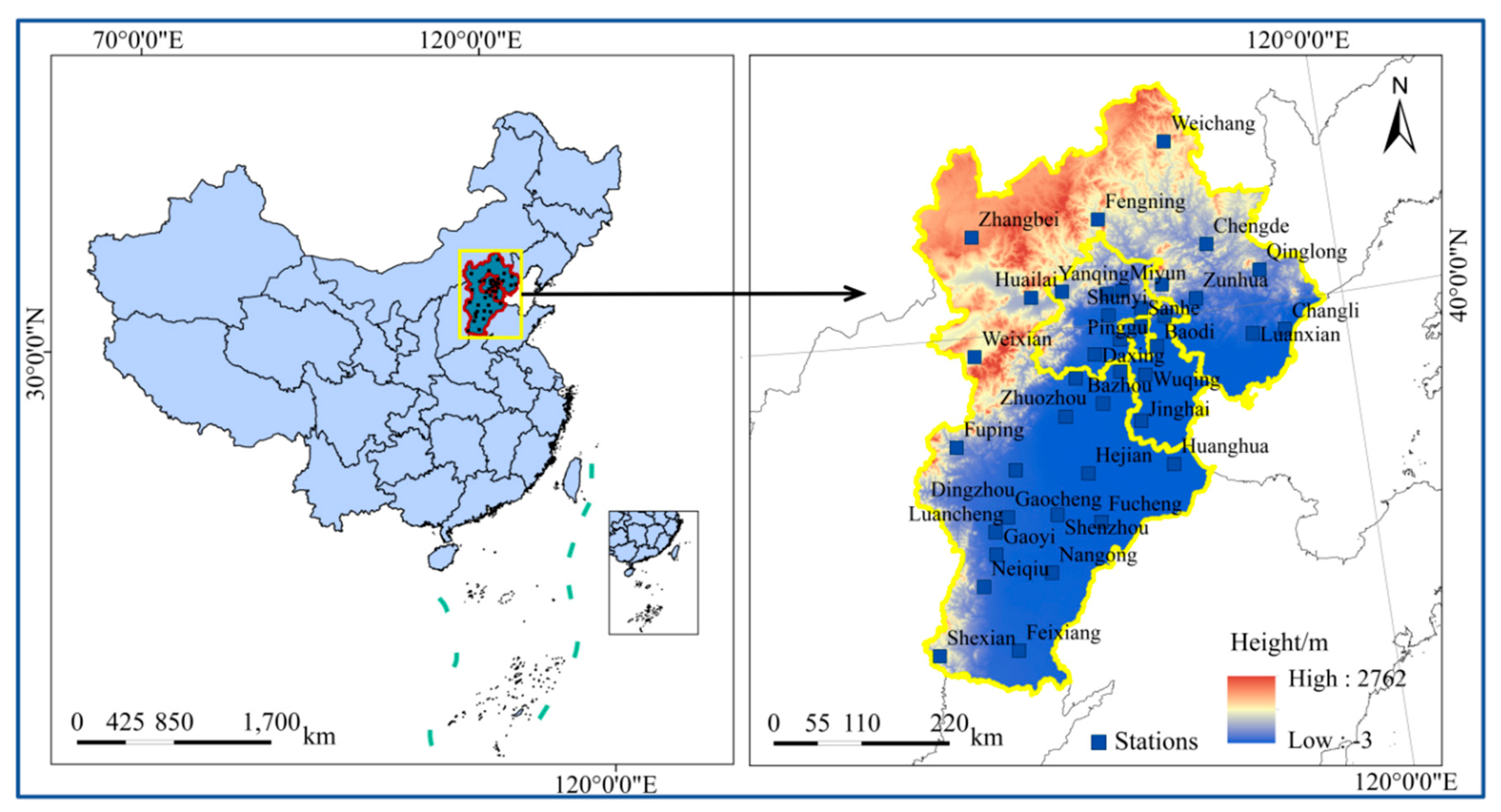
2.1. Overview of the Study Area

The Beijing–Tianjin–Hebei region is the “capital economic circle” of north China, referred to as Jing–Jin–Ji, which surrounds the capital, Beijing. Jing–Jin–Ji, located in the north China plain at 36°01′–42°37′ N, 113°04′–119°53′ E, is bordered from north to south by Neimenggu, Liaoning, Shangdong, Shanxi, and Henan provinces [22]. The climate is a warm temperate monsoon climate, the precipitation and hottest temperatures are concentrated in the summer, the spring and autumn are short, and the winter and summer are long. The research area and site distribution are shown in Figure 1.

2.2. Data Sources and Processing

The meteorological data of this manuscript were obtained from the China Meteorological Data Network (http://data.cma.cn, accessed on 5 July 2021). Daily meteorological data (average temperature, average relative humidity, wind speed, and sunshine daily hours) from 40 meteorological stations in the research area were selected, which are expressed as T, RH, WS, and SSD, respectively. There were 4.38 × 10⁵ data groups. Where parts of the meteorological station daily value data were missing or abnormal, linear interpolation of mean, or median value methods, were used to supplement the missing data, according to the situation. Geographic information include the latitude, longitude, and altitude of each site, as well as the administrative boundaries of the study area. The range of specific meteorological data is shown in

Table 1. Data range of meteorological factors.

Meteorological Factor	T (°C)	RH (%)	WS (m/s)	SSD (h)
Data range	−50~50	0~100	0~20	0~20
Data accuracy	0.1	1	0.1	0.1

.

2.3. FAO-56 Penman–Monteith Equation

The Penman–Monteith formula, recommended in the 1998 FAO-56 paper, was adopted. Based on the principle of energy balance and aerodynamics, the equation has a complete theoretical basis as well as a high calculation accuracy and is widely used across the globe [23]. The Penman–Monteith model is expressed as follows:

$${\mathrm{ET}}_0=\frac{0.408\Delta \left(R_n-G\right)+\gamma \frac{900}{T+273}{U}_2\left(e_s-e_a\right)}{\Delta +\gamma \left(1+0.34U_2\right)},$$

(1)

where ET₀ represents the reference evapotranspiration, mm/d; R_n is the net radiation, MJ/(m²·d); G is the soil heat flux density, MJ/(m²·d); T is the mean air temperature, °C; e_s is the saturated vapor pressure, kPa; e_a is the actual water vapor pressure, kPa; Δ is the slope of the saturation vapor pressure function, kPa/°C; γ is the psychometric constant, kPa/°C; and U₂ represents the wind speed at 2 m height, m/s.

2.4. Climate Tendency Rate

The climate tendency rate reflects the changing trend of climate elements, which can be calculated using linear regression [24]. The calculation formula of the linear regression coefficient (a) sample (Y_i) and time is as follows:

$$Y_i=at+b,$$

(2)

where t, b, and 10 × a are time series, empirical coefficient, and climate tendency rate, respectively.

2.5. Mann-Kendall Trend Testing

The M-K method is a non-parametric statistical test. Compared with parameter tests, the advantage of the M-K trend test is that its sample does not need to follow certain distribution requirements, nor is it affected by a few outliers, so it is more suitable for type variables and sequential variables. The trend analysis method has been used widely in hydrology and meteorology in recent years [25]. In this manuscript, a confidence level of α = 0.05 was used to test the data and find out the change points through the M-K test, and to analyze the trend of meteorological factors and evapotranspiration before, after, and throughout the year.

2.6. Morlet Wavelet Analysis

In time series research, time domain and frequency domain are two commonly used basic forms. Time domain analysis can be calibrated and frequency domain analysis can be used for frequency localization, but neither can reflect the hidden randomness, mutation, and multi-level evolution law with a “multi-time scale” structure in non-stationary sequences. In the early 1980s, Morlet wavelet analysis began to be applied to the study of time series. Morlet wave analysis can, simultaneously, carry out time-frequency domain analysis to reveal various periods of change hidden in time series, reflect the changing trends of the system in different time scales, and make a qualitative estimation of the future development trend of the system [26]. Its function is as follows:

$$\phi \left(t\right)=e^{i{\omega }_{0}t}\cdot e^{-t^2/2},$$

(3)

2.7. Path Analysis

Path analysis is widely used in biological research. This method can not only analyze the relationship between independent variables and dependent variables, but also analyze the mode and degree of the influence of the indirect action between independent variables and dependent variables [27]. In this manuscript, SPSS software was used to determine the direct and indirect path coefficients of each meteorological factor to the ET₀, so as to qualitatively study the main meteorological factors affecting the ET₀. The main calculation formula is:

$$r_{iy}=p_{yi}+{\displaystyle \sum _{j=i+1}^n{r}_{ij}}{p}_{yj},$$

(4)

2.8. Sensitivity Analysis

The relationship between ET₀ and climate factors is very close. In order to quantitatively describe the impact of climate factors on ET₀, the sensitivity coefficient analysis method and contribution rate assessment are, generally, used. Partial derivative sensitivity coefficient analysis is a method of global sensitivity analysis that controls the influence of other parameters and obtains the correlation between input factors and output results [28,29]. The sensitivity analysis was first proposed by McCuen, to calculate the partial derivative of the ET₀ to each meteorological factor, that is, to calculate the ratio of the relative change of the ET₀ to the relative change of a single meteorological factor [30]. The specific calculation formula is:

$$S_{v_i}=\underset{\Delta \to 0}{\lim }\left(\frac{\Delta {\mathrm{ET}}_0}{\Delta v_i}\cdot \frac{{\mathrm{ET}}_0}{\partial v_i}\right)=\frac{\partial {\mathrm{ET}}_0}{\partial v_i}\cdot \frac{v_i}{{\mathrm{ET}}_0},$$

(5)

where v_i is the meteorological factor; S_vi is the sensitivity coefficient; ΔET₀ and Δv_i are the change values of ET₀ and meteorological factors, respectively; and positive or negative S_vi values indicate that ET₀ increases or decreases, respectively, with the increase in meteorological factors. The meteorological factor sensitivity coefficients were expressed as S_T, S_RH, S_WS, and S_SSD, in this study.

2.9. Contribution Rate Analysis

The change in ET₀ is not only affected by the sensitivity of its climate factors, but also relates to the change degree of each climate factor. To determine the cause of the change in ET₀, it is necessary to combine the sensitivity analysis with the actual changes in climate elements. Thus, it is significant to find the contribution rate to ET₀ of a single climate factor. The contribution of meteorological factors to ET₀ can be obtained by multiplying the sensitivity coefficient with the annual relative change rate of the factor [31]:

$$G{X}_{v_i}=S_{v_i}\cdot R{C}_{v_i},$$

(6)

$$R{C}_{v_i}=\frac{n\cdot Tren{d}_{v_i}}{\left|a_{vi}\right|}\times 100\%,$$

(7)

$$R{C}_{{\mathrm{ET}}_0}=\frac{n\cdot Tren{d}_{v_i}}{\left|a_{v{\mathrm{ET}}_0}\right|}\times 100\%,$$

(8)

where GX_vi is the contribution of meteorological factors to ET₀ change; RC_vi is the years of relative rate of change of factors; ${RC}_{\mathrm{E}{\mathrm{T}}_0}$ is the ET₀ years relative rate of change, that is, the actual rate of change; n is the total year; Trend_vi is the annual change rate of the meteorological factor vi; and the linear tendency rate of this factor for many years, which is calculated from the trend analysis of univariate linear regression between vi and n, is a_vi for the multi-year average of the factors. The contribution rates of temperature, relative humidity, wind speed, and sunshine hours to ET₀ change were marked as GX_T, GX_RH, GX_WS, and GX_SSD. The summation of contribution is G_SUM = GX_T + GX_RH + GX_WS + GX_SSD. Through analyzing the contribution rate of each factor to the ET₀, the influence of each meteorological factor on the ET₀ could be quantitatively studied.

2.10. Inverse Distance Weighted Interpolation

The inverse distance weighted interpolation (IDW) method in ArcGIS10.2 (ESRI, Redlands, CA, USA) was used to study the spatial distribution of regional ET₀. IDW is a common and simple spatial interpolation method. It is based on the principle of similarity, that is, the closer two objects are, the more similar their properties are. The distance between the interpolation point and the sample point is a weighted average, and the weight is given to the sample point [32]. The spatial distribution of ET₀ and meteorological factors in the Beijing–Tianjin–Hebei region were analyzed using IDW.

3. Results

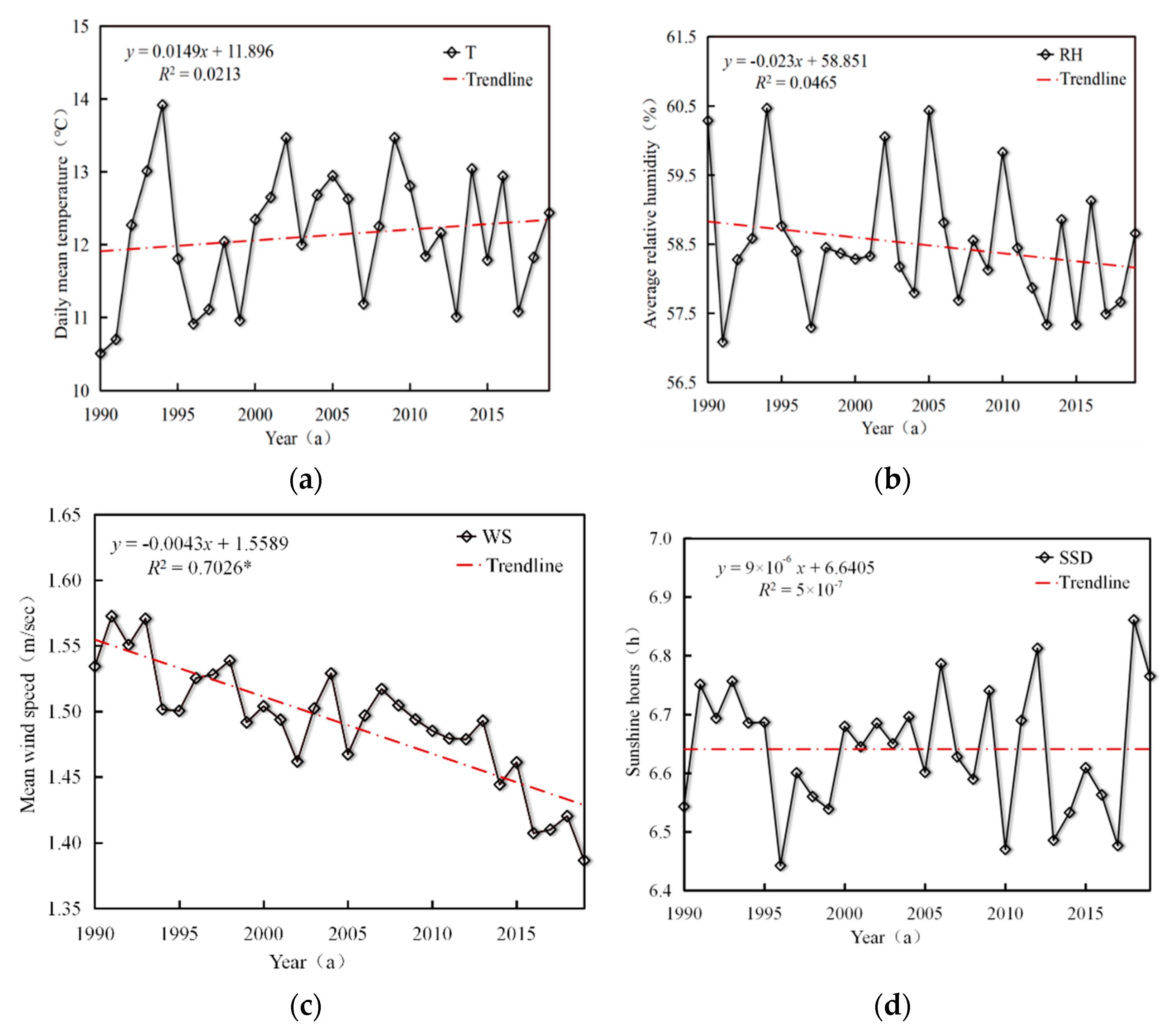
3.1. Temporal Variation of Meteorological Factors

The interannual variation trend of various meteorological factors is shown in Figure 2. It can be seen that the interannual changes of various meteorological factors in the Beijing–Tianjin–Hebei region were uneven, and the curve as a whole showed volatile changes. Except for WS, the change trend of other meteorological factors was not significant. T had an upward trend during the 1990–2019 evolution, with a climatic tendency rate of 0.15 °C/10 a., and the average annual T was 12.1 °C. Overall, the annual average RH was 58.5%, the climate tendency was −0.28%/10 a, and there was no obvious change trend. The overall average WS at 2 m showed a downward trend, below the average of 1.49 m/s at the beginning of the 21st century, with an average reduction of 0.043 m/s per 10 a. The overall change in SSD was not significant. The maximum SSD was 6.86 h in 2018, the minimum was 6.44 h in 1994, and the average over the years was 6.64 h, with a change range of 0.22.

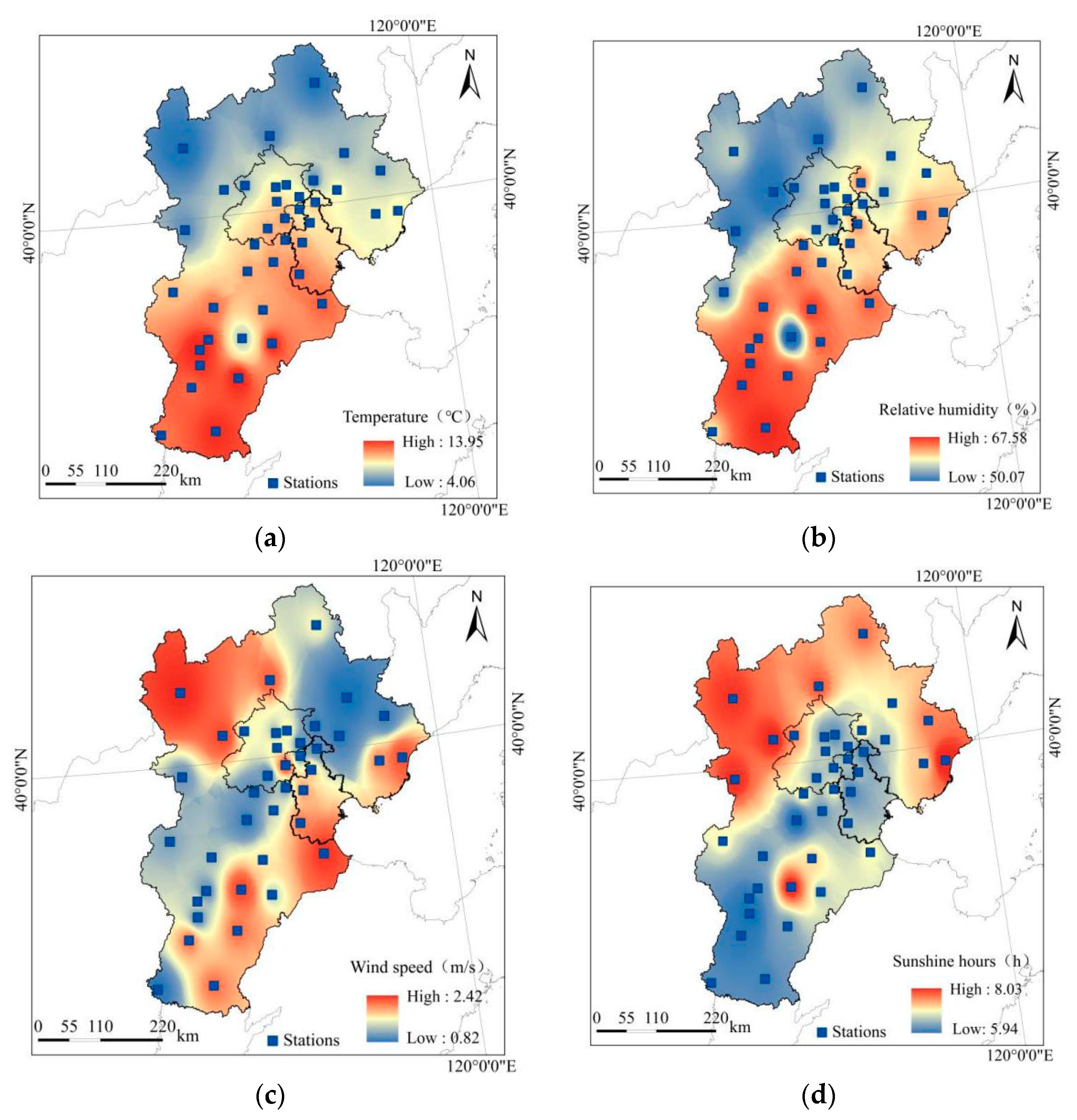
3.2. Spatial Distribution of Meteorological Factors

It can be seen from Figure 3 that the distribution of meteorological factors in the Beijing–Tianjin–Hebei region was spatially variable. The WS distribution had longitudinal zonal characteristics, and the T, RH, and SSD differed with latitude. Specific analysis shows the average T range was 4.1–14.0 °C, which is relatively large. The highest-value areas were in southern Hebei as well ascentral and southern Beijing and Tianjin, with an average of 14.3 °C. The T in the Weichang area was relatively low, due to its high altitude and monsoon plateau mountain climate. The average T in the Zhangbei area was only 4.1 °C, since it is located on the dam on the southern edge of the Inner Mongolia Plateau. The RH ranged from 50.1% to 67.6%, the difference between high and low values was 17.5%, showing a relatively large difference. The high-value areas were, mainly, distributed in Feixiang and Gaoyi in southern Hebei province, at 67.6% and 65.3%, respectively. The low-value centers were distributed in Huailai and Fengning in northern Hebei as well as Shenzhou in southern Hebei, at an average of 51.2%. The average WS ranged between 0.82 m/s and 2.42 m/s. Zhangbei and Huailai stations had a high WS because of their high altitude, while the other high-value centers appeared in the southeast of the Beijing–Tianjin–Hebei region, especially Changli, Tongzhou, and Jinghai, with WS of 1.88 m/s, 1.86 m/s, and 1.67 m/s, respectively. The total range of SSD was 5.9–8.0 h. The highest value locations were 8.03 h, 7.90 h, and 7.89 h in Changli, Hailai, and Shenzhou, respectively, while Neiqiu, Gaoyi, and Rongcheng had lower annual SSD, with an average of 6.02 h.

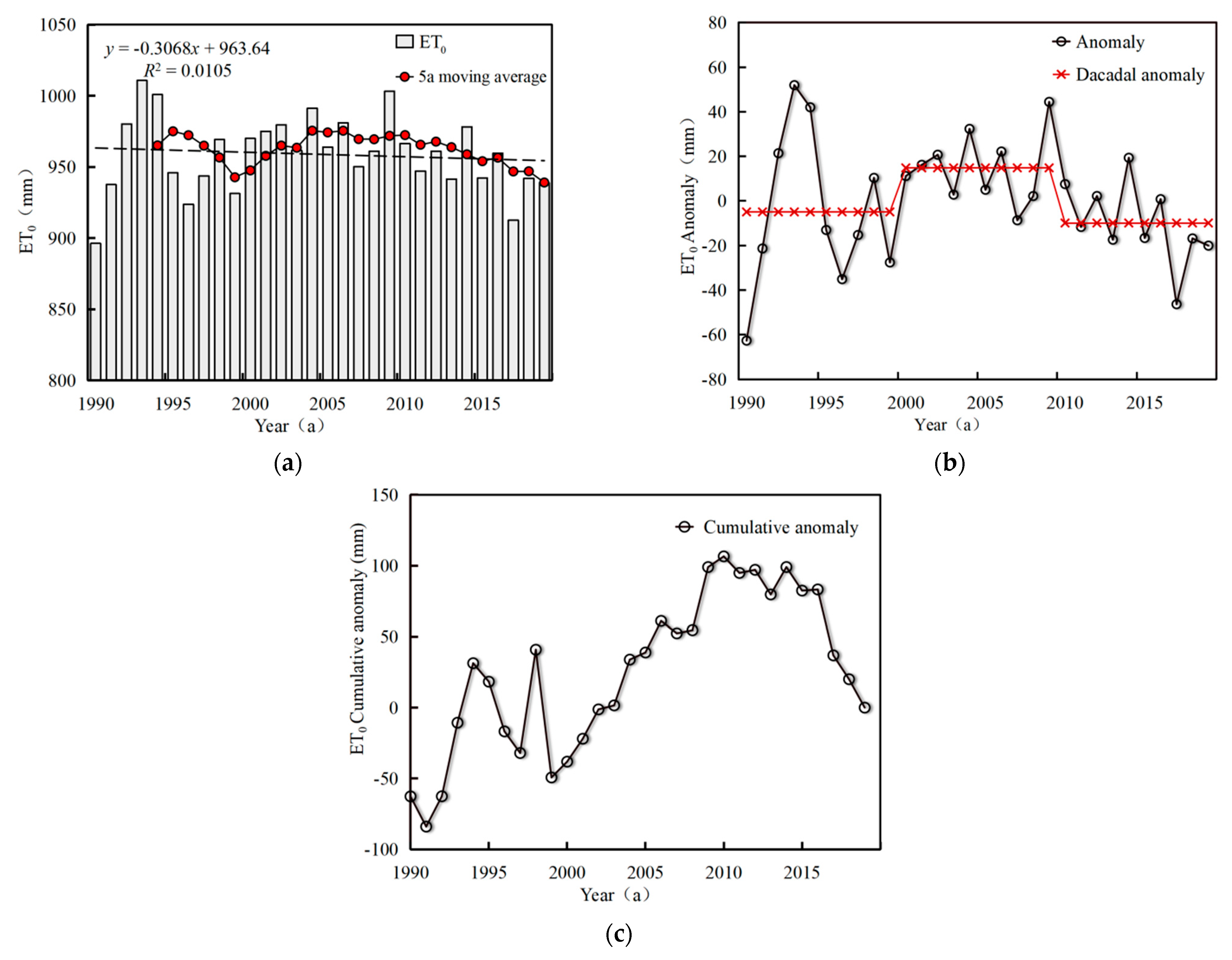
3.3. Temporal Variation of ET₀

The average annual ET₀ of the Beijing–Tianjin–Hebei region, from 1990 to 2019, showed an insignificant downward trend, at a rate of −3.07 mm/10 a. The maximum interannual ET₀ was in 1993, at 1010.80 mm, while the lowest was in 1990, at 894.24 (Figure 4a). There was a fluctuating downward trend until 2009, maintaining a downward trend after that. With respect to inter-decadal variation, as shown in Figure 4b, the ET₀ went upward, first, and, then, declined from the 1990s to the 2010s, with a range of 19.76 mm and 24.72 mm per decade. The 1990s and 2010s showed a negative anomaly, which was least in the 2010s. The 2000s showed a positive anomaly, which was largest in the 2010s, with the decadal anomaly at −9.90 mm. The accumulated anomaly of annual ET₀ was variable but, generally, upward, as shown in Figure 4c, peaking in 2010, then gradually decreasing until the end of the 2010s.

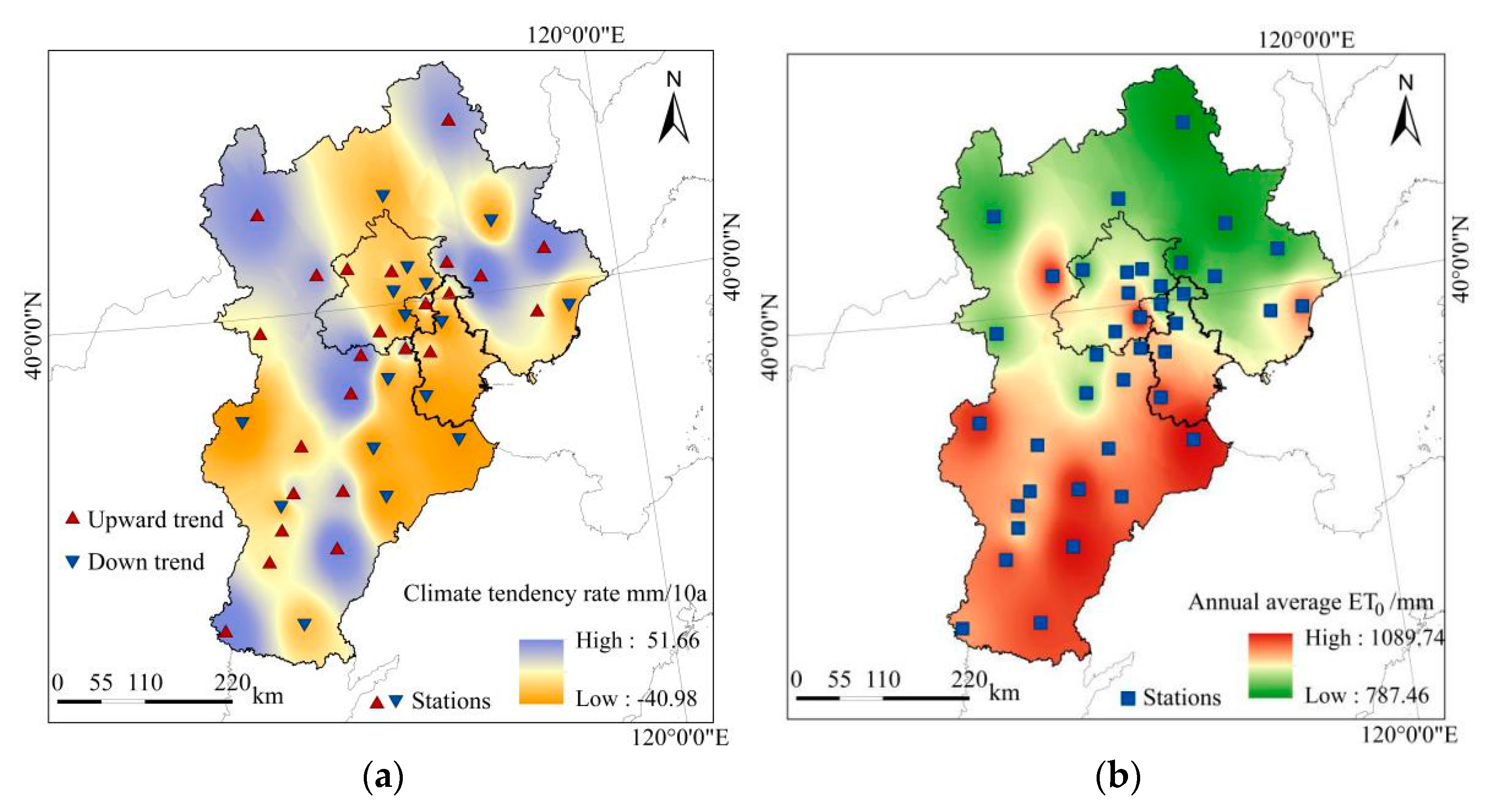
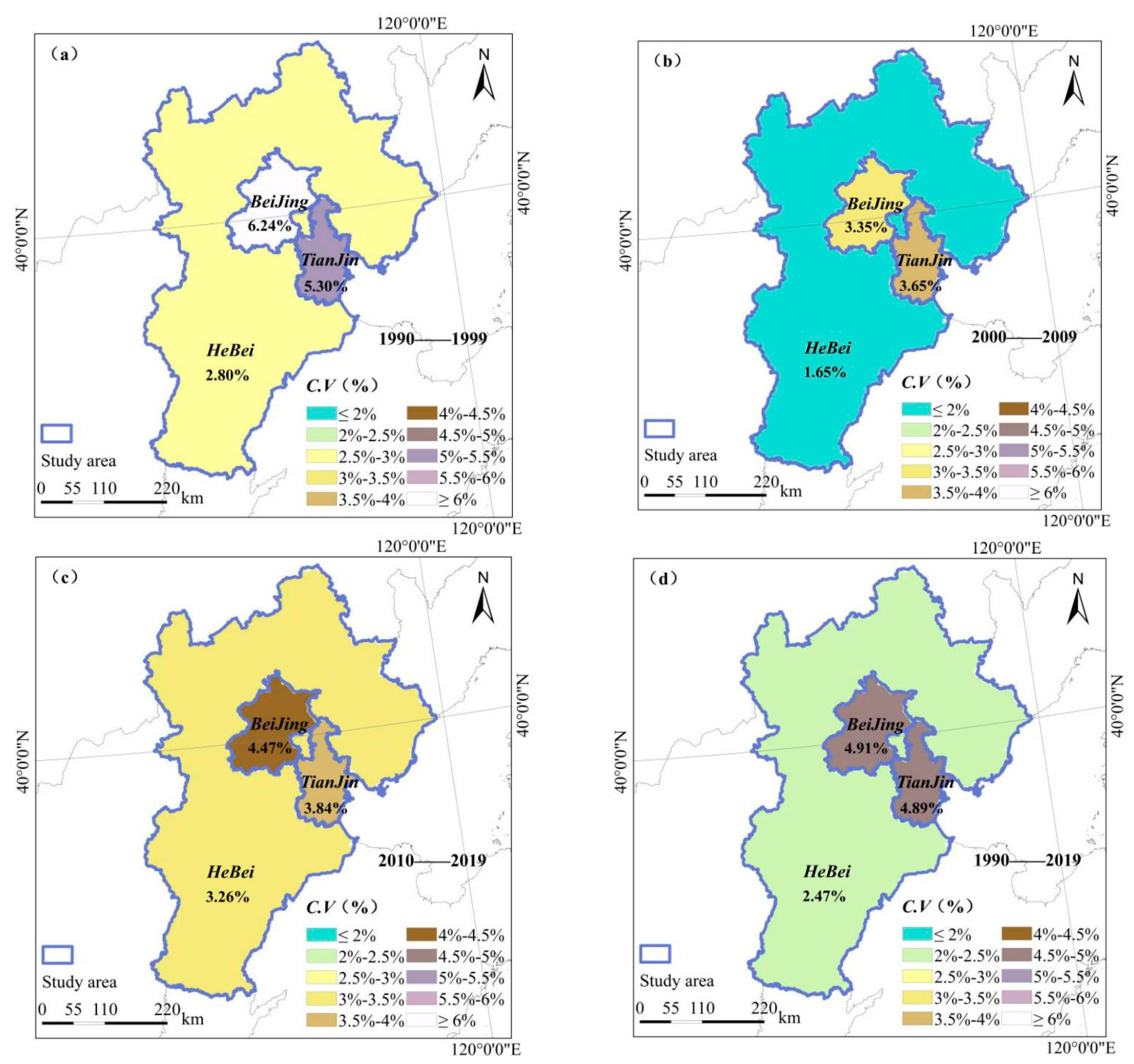
3.4. Spatial Distribution of ET₀

The ET₀ of 16 sites (40%) in the Beijing–Tianjin–Hebei region showed a downward trend (Figure 5a). Among which, Tongzhou, Fuping, and Huanghua station’s ET₀ showed a large negative climate tendency rate, of −41.18, −39.02, and −32.00 mm/10 a, respectively. Twenty-four sites showed an upward trend (60%), among which the ET₀ of Zunhua, Rongxian, and Shexian showed a large upward trend, of 51.72, 44.69, and 44.19 mm/10 a, respectively. Overall, the spatial distribution of ET₀ from 1990 to 2019 was not uniform. As shown in Figure 5b, the high value interannual ET₀ areas were, mainly, distributed in southern Hebei, southeastern Beijing, and southern Tianjin. The values in the northern and northeastern Beijing–Tianjin–Hebei area were relatively low. The spatial distribution characteristics of ET₀ at each local site varied because of their geographical location and climate environment. The high-value areas were, mainly, distributed in Huanghua, Nangong, and Tongzhou, with ET₀ values of 1089.83, 1078.30, and 1064.09 mm, respectively. Huanghua and Nangong are located on the eastern part of the North China Plain, with longer sunshine and lower rainfall, so the ET₀ is higher, while Tongzhou is located in the Beijing suburbs, which is affected by a cold current in autumn and winter, with a high wind speed and humidity, so the ET₀ is higher. The areas with low ET₀ values were, mainly, distributed in Weichang and Xinglong, with values of 803.98 and 786.45 mm, respectively. Weichang is located in the northernmost part of Chengde, which belongs to a monsoon-type plateau mountain climate, with higher elevation and lower temperature, so the ET₀ was lower. The eastern end of Jiaodong Peninsula faces the sea, so the low T leads to low ET₀, while Xinglong has low ET₀ because of the abundant rainfall on the towering terrain.

3.5. The Trend Test of ET₀

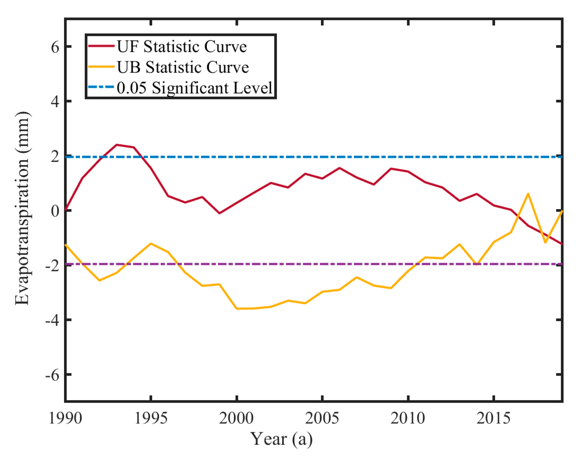
3.5.1. Mann-Kendall Trend Test

To explore the reasons for the overall downward trend of annual ET₀ in the Beijing–Tianjin–Hebei region, the M-K trend method was used to test the annual ET₀. The UF curve represents the time series, and the UB curve shows the trend statistics of the inverse sequence in the reverse time series (Figure 6). If the value of the UF curve is greater than 0, the time series shows an upward trend. The UF and UB intersection point, with the line showing significance at 0.05, indicates an effective change. Figure 6 shows that the UF and UB curve of the interannual ET₀ of the study area intersected in 2016 and 2017, indicating that the ET₀ began to mutate in 2016, and a change occurred in 2016–2017. The calculated decrease was 47.12 mm.

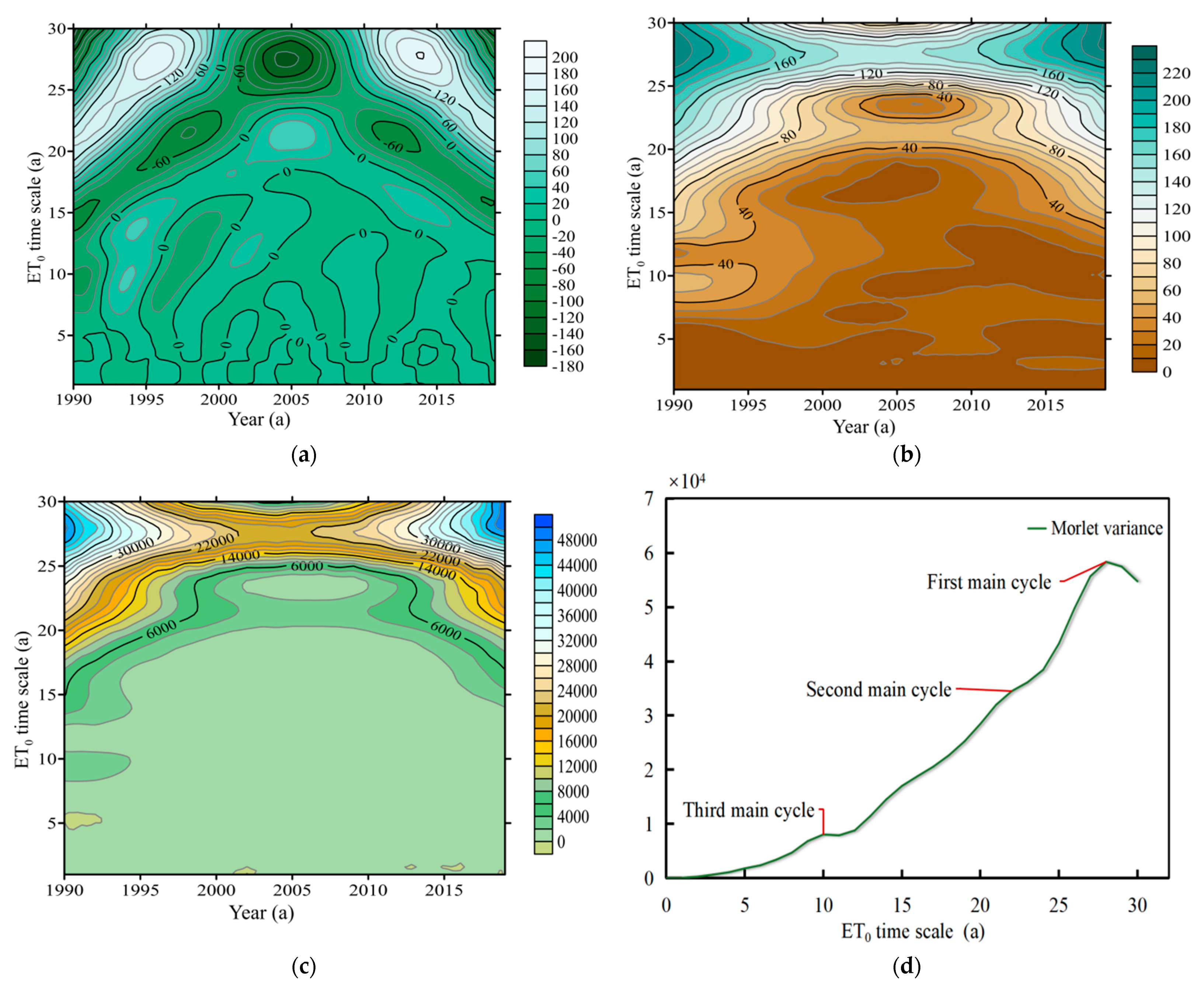
3.5.2. Morlet Wavelet Periodic Inspection

In order to further reveal the multi-time scale evolution law of ET₀, the interannual ET₀ was analyzed by Morlet wavelet. From Figure 7a, it can be seen that there were 22–28 main oscillation cycles, in the evolution of the ET₀ during 1990–2019. There were two overcenters across the time scale, in 1996 and 2014, and three undercenters in 1998, 2005, and 2012. The modulus value of the Morlet wavelet coefficients is the reflection of the distribution of energy density, corresponding to different time scale periods in the time domain. The larger the coefficient modulus value is, the stronger the periodicity of the corresponding period or scale. Thus, as shown in Figure 7b, in the process of ET₀ evolution, the time scale modulus value of 24–28 years was the largest (more than 160), but the modulus value between 2000 and 2010 was 140, which indicated that the periodic change of the 24–28 years’ time scale was not obvious during this period. After 2010, the model value increased again, and the periodic change of the time scale of 24–28 years after this period tended to be significant. The mode of wavelet coefficient is equivalent to wavelet energy spectrum, which can analyze the oscillation energy of different periods. Figure 7c shows that the energy of 24–28 years was the strongest, and the period was the most significant, but its periodic change was local (before 2000 and after 2010). The time scale energy of 5–12 years was weak, but the periodic distribution was obvious, occupying almost the whole study-time domain (1990–2019). A wavelet variance graph can reflect the distribution of fluctuating energy with the scale (a) of the time series and can be used to determine the main period that exists during ET₀ evolution. Figure 7d has three obvious peaks, which correspond to the time scales of 10 a, 22 a, and 28 a, from small to large. The maximum peak value corresponded to the time scale of 28 a, indicating that the periodic oscillation of about 28 a (time scale) was the strongest, which was the first main period of annual ET₀ change; the second peak corresponded to the time scale of 22 a, the second main period; and the third peak corresponded to the time scale of 10 a, the third principal period of the ET₀. These showed that the fluctuations of the aforementioned three cycles controlled the ET₀ variation characteristics over the whole time domain.

3.6. Effects of Meteorological Factors on ET₀ Analysis

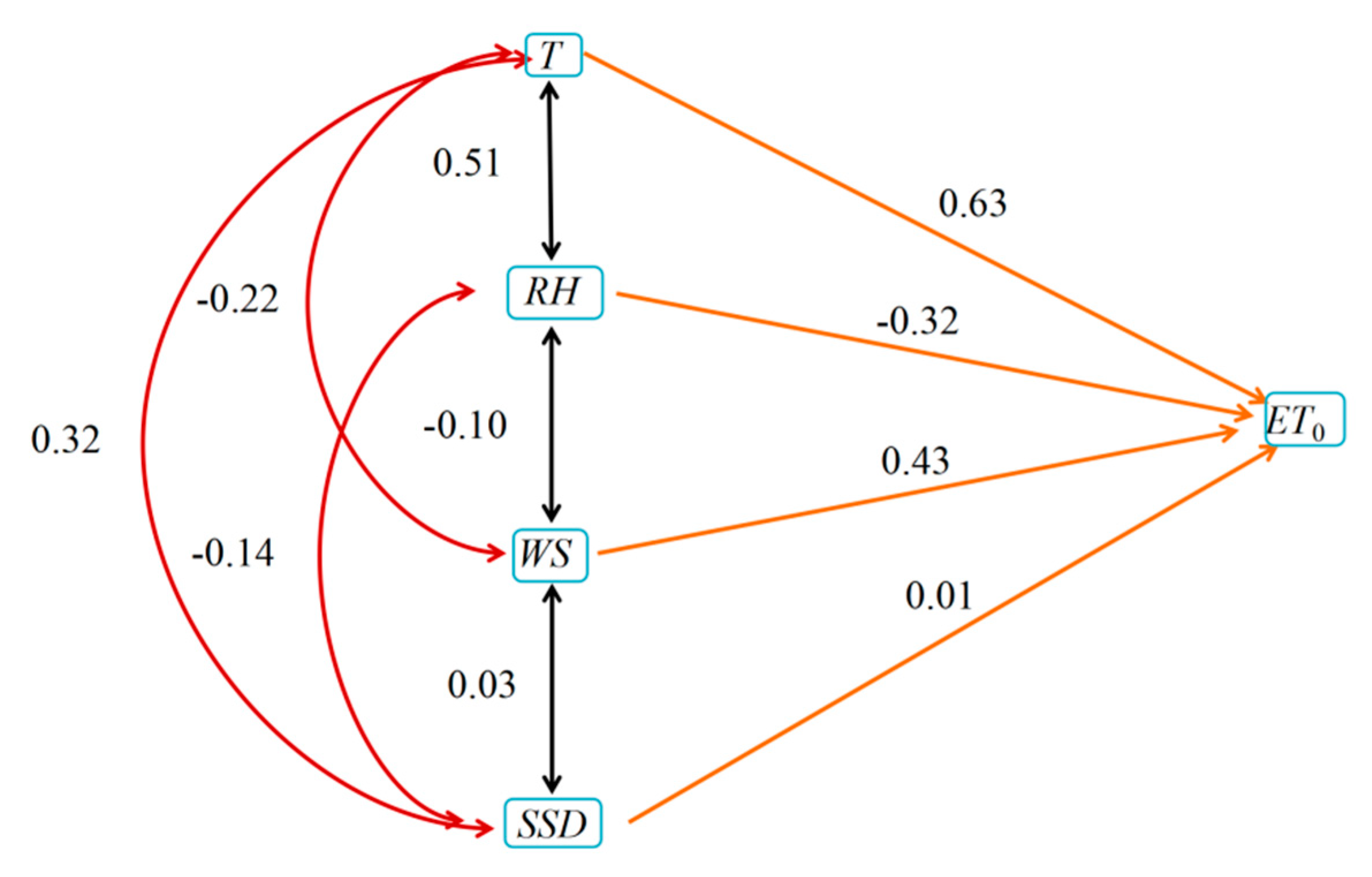
3.6.1. Path Analysis of Each Meteorological Factor on the Annual Average ET₀

By means of path analysis, the influence of meteorological factors on ET₀ was further analyzed. Path analysis decomposes the correlation coefficient into a direct path coefficient (the direct effect of an independent variable on the dependent variable) and indirect path coefficient (the indirect effect of the independent variable on the dependent variable through other independent variables), which can clarify the direct and indirect effects of meteorological factors on ET₀ changes. The specific results are shown in

Table 2. Path coefficients of factors on annual ET₀.

Factors	Coefficients	Direct Path Coefficients	Sum of Indirect Path Coefficients	Indirect Path Coefficients				Decision-Making Coefficients
				T	RH	WS	SSD
T	0.856	0.630	−0.287	-	−0.200	−0.090	0.003	0.340
RH	−0.204	−0.323	0.070	0.322	-	−0.043	−0.001	−0.045
WS	0.212	0.418	−0.100	−0.135	0.033	-	0.005	0.318
SSD	0.405	0.008	0.2575	0.204	0.044	0.010	-	0.270

and Figure 8. The direct path coefficient of WS for the annual average ET₀ was 0.42, while the correlation coefficient was only 0.21. This was because the T inhibited ET₀ by influencing the WS coefficient, with indirect path coefficients of −0.135. The direct diameter coefficient (0.63) of T was larger, the correlation coefficient (0.86) was larger, and the indirect diameter coefficient (−0.29) was smaller, which indicated that the influence of T on ET₀ was, mainly, through direct action. The correlation coefficient of the SSD was high (0.41), and the direct path coefficient was low (0.01), since T, RH, and WS inhibited ET₀ through the WS influence; their indirect path coefficients were 0.20, 0.04, and 0.01, respectively. The T promoted SSD. Since the indirect path coefficient of SSD was 0.26, the sum of the direct path coefficient was smaller (0.01). The correlation coefficient between RH and ET₀ was -0.204, and its absolute value was large, mainly since the indirect diameter coefficient played a major role. The ranking of decision coefficients was T > WS > SSD > RH, indicating that T ’s comprehensive decision ability to change ET₀ was greater.

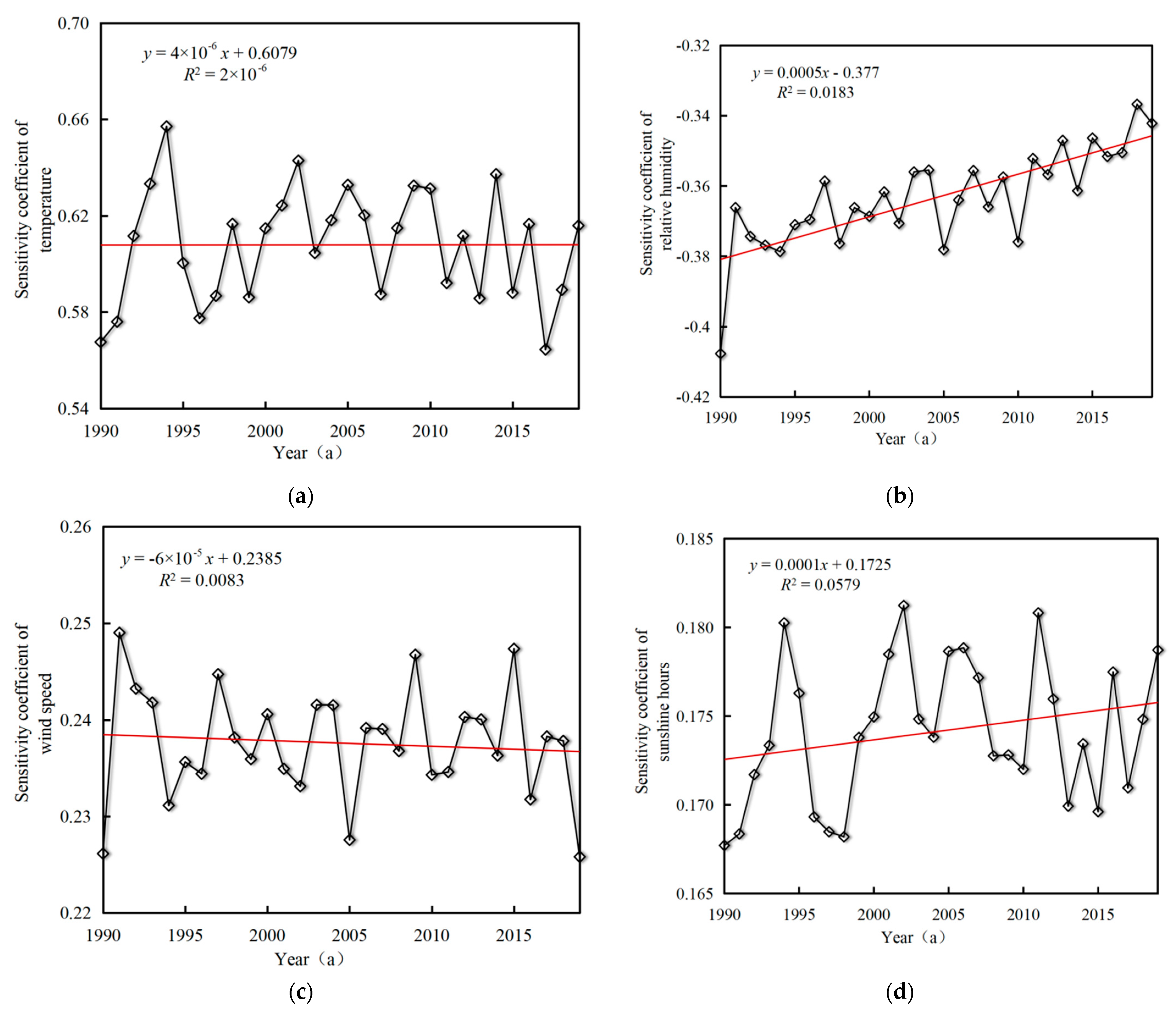
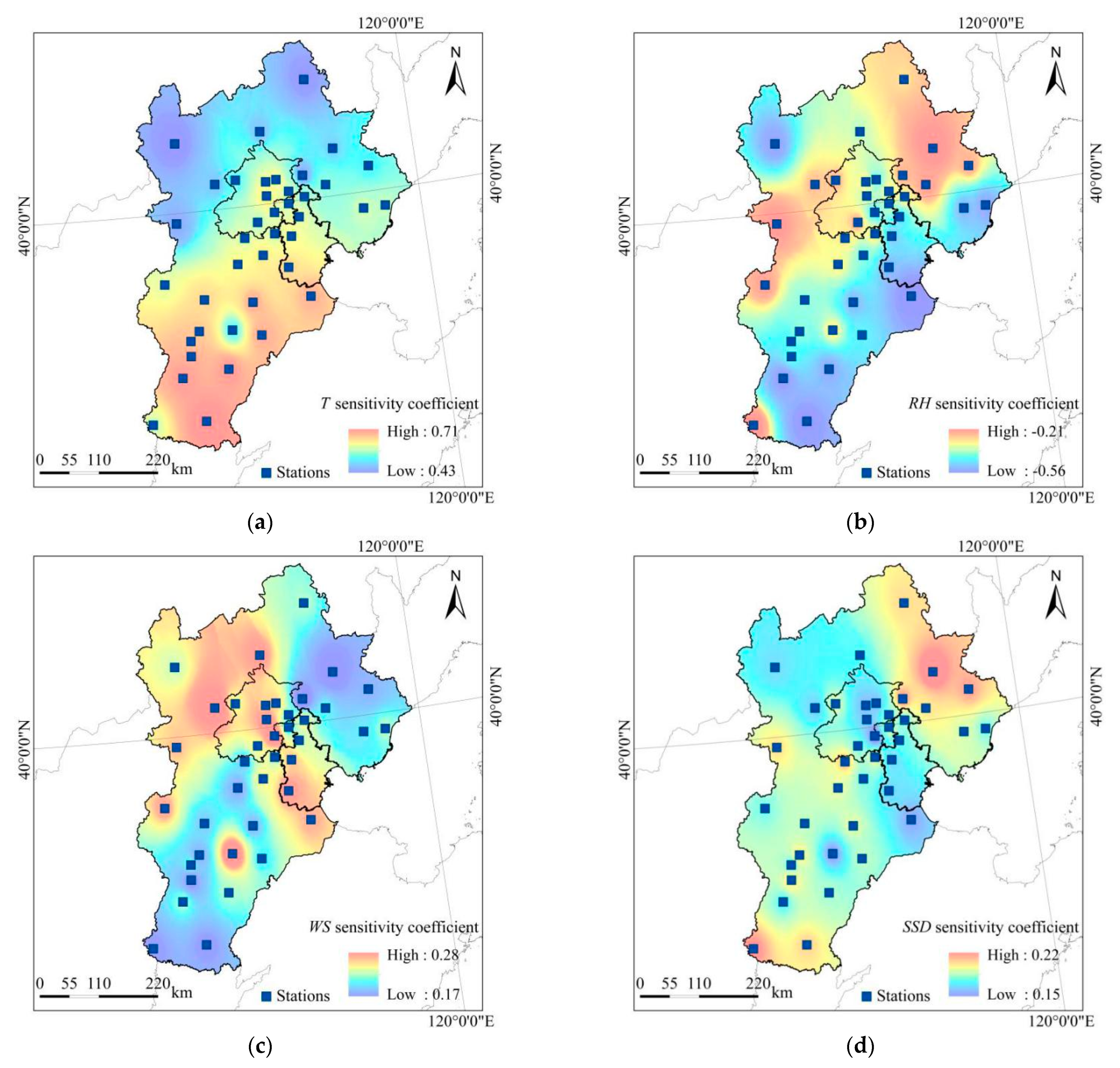
3.6.2. Sensitivity Analysis of Each Meteorological Factor on the Annual Average ET₀

The sensitivity coefficient of the ET₀ for each meteorological factor is shown in Figure 9. It can be seen that the S_T, S_WS, and S_SSD were all positive, which indicated that the ET₀ increased with the increase in T, WS, and SSD, while the S_RH was negative, indicating that the ET₀ decreased with the increase in RH. The absolute value of the sensitivity coefficient showed that the ET₀ was the most sensitive to T, followed by RH, and the least sensitive to SSD. From the point of temporal variation, the S_WS interannual curves showed a downward trend, while the S_T, S_RH, and S_SSD interannual curves showed an upward trend. The climate tendency rates of S_T, S_RH, S_WS, and S_SSD were −0.005, 0.005, −0.003, and 0.001/10 a, respectively. The temporal variation trends of S_T, S_RH, S_WS, and S_SSD were not significant.

Sensitivity analysis was carried out between the meteorological factors and the annual average ET₀ of each meteorological station in the Beijing–Tianjin–Hebei region, from 1990 to 2019, and the spatial distribution characteristics of the sensitivity coefficients between each meteorological factor and the annual average ET₀ were analyzed (as shown in Figure 10). In general, the spatial distribution of the sensitivity coefficients between the annual average ET₀ and each meteorological factor is different. Among them, the spatial distribution of S_T and S_WS has zonal characteristics, S_RH shows a trend of first increasing and then decreasing along the southeast to northwest direction, and S_SSD is, generally, high in the north–south direction at both ends and low in the middle. From a numerical point of view, the absolute value of the spatial distribution of the sensitivity coefficients of each meteorological factor to ET₀ is in the descending order of S_T > S_RH > S_WS > S_SSD. From a local point of view, the spatial distribution of the sensitivity coefficient S_T ranges from 0.43 to 0.71, and the high-value areas of the sensitivity coefficient are, mainly, distributed in Feixiang and Neiqiu in southern Hebei, Gaoyi and Nangong in central Hebei, and other places, with a mean value of 0.69. The low-value areas are concentrated in Zhangbei and Weichang in northern Hebei, with 0.431 and 0.451, respectively (Figure 10a). The variation range of the sensitivity coefficient S_RH ranges from −0.56 to −0.21, and the areas with larger absolute values are concentrated in the Huanghua, Feixiang, and Changli areas, with an average value of −0.49 (Figure 10b). The sensitivity coefficient of S_WS varies from 0.17 to 0.28. The high-value areas are, mainly, Tongzhou in Beijing, Shenzhou in Hebei, and Jinghai in Tianjin, with an average value of 0.27 (Figure 10c). The sensitivity coefficient of S_SSD varies from 0.15 to 0.22. The high-value areas are, mainly, concentrated in the Chengde and Xinglong areas in Hebei, while the low-value areas are distributed in Tongzhou in Beijing and Huanghua in Hebei, with a sensitivity coefficient of 0.148, 0.157, and 0.160, respectively (Figure 10d).

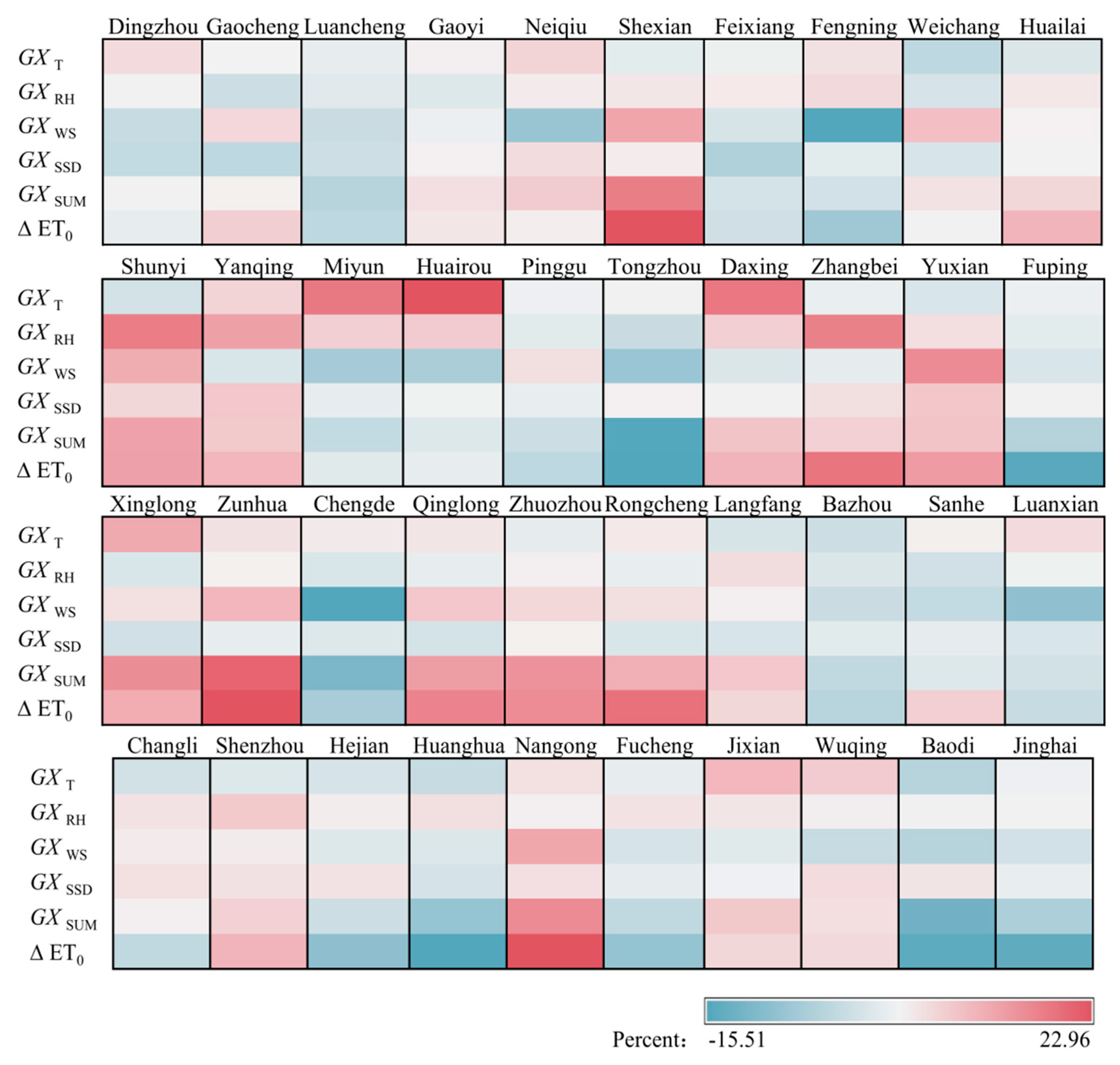
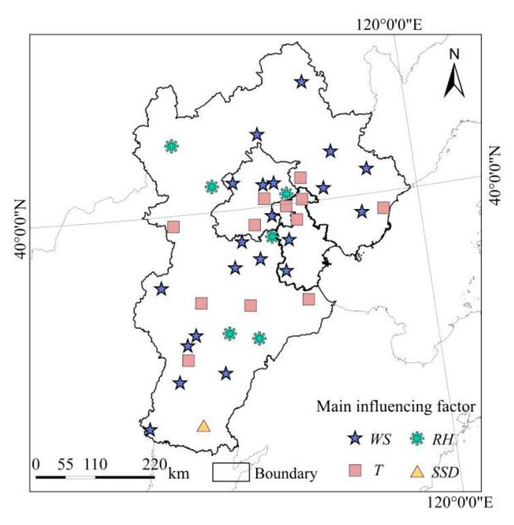
3.6.3. Contribution Rate Analysis between Meteorological Factors and ET₀

The contribution rate analysis method is used to further quantify the impact of each meteorological factor on the change of ET₀. Multiply the sensitivity coefficient (S_vi) of the station ET₀ for each meteorological factor by the multi-year relative change rate (RC_vi) of the meteorological factor, to obtain the contribution rate (Con_vi) of each meteorological factor for the multi-year change of ET₀. The contribution-rate heat map of meteorological factors at each station is shown in Figure 11. The results of path analysis show that WS and T are the dominant meteorological factors affecting the change of ET₀ in the Beijing–Tianjin–Hebei region. The comprehensive influence degree of RH and SSD is not high, and the contribution rate of each meteorological factor is WS > T > RH > SSD, from high to low. Among them, Zunhua, Shexian, and Nangong have the highest contribution rates of WS, which are 10.78%, 9.43%, and 8.61% respectively. Chengde and Luan counties have a relatively low contribution rates of WS, with an average of 13.23%. Xinglong, Luanxian, and other places have a relatively high T contribution rate, with an average of 9.41%. The low contribution rate is distributed in Xinglong and other places, with 4.94% and 2.65%, respectively. The overall change of the RH contribution rate of each station is small, except that Langfang and Fengning are 5.96% and 3.88%, respectively, so the change range is 4.86~5.96%. The high-value areas for SSD contribution rate are located in Neiqiu and Zhuozhou, with an average of 3.45%. The low-value areas are concentrated in Feixiang and Huanghua, with 3.04% and 3.79%, respectively (Figure 12).

4. Discussion

The fifth Intergovernmental Panel on Climate Change (IPCC) report indicated that between 1880 and 2012, the average global warming was 0.85 ± 0.2 °C. In response, research into regional climate systems in the context of global warming has become a focus [33]. The atmospheric evapotranspiration capacity can be characterized by ET₀, which is a basic parameter for estimating crop-water demand and is an important index for evaluating the degree of regional drought, water consumption by vegetation, and water-supply-and-demand balance [34]. As an important economic center of gravity and agricultural production area in China, the Beijing–Tianjin–Hebei region has gradually accelerated its integration process, since the 1990s. Therefore, the temporal and spatial variation characteristics of ET₀ in the Beijing–Tianjin–Hebei region in the past 30 years as well as the impact of meteorological factors on its changes were analyzed, in order to guide the rational irrigation in the region and enhance the adaptability of agricultural production, to cope with climate change and the ability to resist climate disasters.

In terms of analyzing the periodic change trend of ET₀, the research in this paper shows that there is a main oscillation period of 24~28 a, in the time evolution of ET₀ in the Beijing–Tianjin–Hebei region, in the past 30 years. The sequence is extended for the first 17 years and the last 17 years, while the “boundary effect” is reduced in the later period, so the main oscillation cycle occupies almost the entire time series. Over the entire time scale, there are, alternately, more centers and fewer centers, which are evenly distributed and may be related to the El Niño and La Niña phenomena that affect the atmospheric water cycle and potential evapotranspiration, affecting regional rainfall and evapotranspiration to some extent throughout the year. The variation characteristics of the annual ET₀ in the entire time domain are controlled by the periodic fluctuations of 28 a, 22 a, and 10 a, respectively, indicating that the ET₀ in the Beijing–Tianjin–Hebei region, in the past 30 years, does not change in a fixed time period, instead changing in the form of multi-cycle nesting of different lengths.

When studying the spatial distribution of ET₀ and its influencing factors in the Beijing–Tianjin–Hebei region during the past 30 a, it was found that the spatial distribution of WS had obvious longitude characteristics, while the difference among T, RH, and SSD was related more to latitude. There were clear differences in the spatial distribution of the meteorological factors. Further, through the spatial change trend map, the distribution characteristics of each meteorological factor were analyzed, so as to analyze the climatic conditions in the Beijing–Tianjin–Hebei region. Figure 13 shows that T on the X-axis (in the east–west direction) has a slight downward trend, of approximately a straight line, indicating that the T in eastern Hebei, Beijing, and Tianjin is, generally, smaller than that in the western region. This is due to the eastern part of the Beijing–Tianjin–Hebei region being, generally, in the flat terrain of the North China Plain, while the Taihang Mountains stretch in the western region, which is easily affected by the monsoon climate, resulting in a lower average temperature. On the Y-axis, T is low in the north and high in the south. This is consistent with the low T in Weichang, Zhangbei, and other places in northern Hebei. The average value is only 4.1 °C (Figure 13a). The RH shows an approximate ∩-shaped trend, high on both sides and low in the middle, along the meridian. Among them, the RH in the eastern Hebei area is greater than the RH in the mountainous areas of southwestern Hebei because of proximity to the Bohai Sea (Figure 13b). The overall trend of WS decreases first and, then, increases from southeast to northwest. Except for the high wind speed in the northwest of Hebei, due to the high terrain, the rest of the high-value centers appear in the coastal east and southeast of Hebei, and the southeast of Hebei is affected by the monsoon climate with high wind speed (Figure 13c). SSD shows a gradual increasing trend from southeast to northwest in the Beijing–Tianjin–Hebei region; the change range is 5.94~8.03 h, and the overall change is not large. This is due to the Beijing–Tianjin–Hebei region being located in the North China Plain. Except for the Taihang Mountains and Yanshan regions, the overall altitude difference within the region is not large, resulting in a small change in SSD (Figure 13d). This was consistent with the spatial distribution of ET₀ and its influencing factors in the Beijing–Tianjin–Hebei region, by Bi et al. [35].

In general, the inter-annual ET₀ in the Beijing–Tianjin–Hebei region follows the distribution characteristics of decreasing from east to west and from south to north, while the spatial variation trend of interannual ET₀ is, obviously, different. Therefore, the spatial variation trend map is used to further analyze its distribution characteristics. As shown in Figure 13e, the interannual ET₀ shows an approximate ∩-shaped variation trend along the meridian direction, low on both sides and high in the middle, and it follows a gradually decreasing trend from south to north, in the latitude direction. Therefore, the high-value areas of interannual ET₀ are, mainly, distributed in southern Hebei, southeastern Beijing, and central and southern Tianjin, while the values in the northern and northwestern regions are relatively small. The spatial variation trend of T is roughly the same as that of the interannual ET₀, both showing a decreasing trend from east to west and from south to north. This can explain the reason for the interannual ET₀ spatial variation trend, which is, mainly, affected by T, resulting in a spatial variation trend similar to that of T. Combining path analysis and contribution rate analysis, to explore the relationship between ET₀ and its impact factors, the results show that except for RH, the sensitivity coefficients between other meteorological factors and ET₀ are all positive; that is, the increase in meteorological factors will lead to the increase in ET₀. Among them, the correlation between T and ET₀ is the most significant, reaching 0.63, and the sensitivity coefficients between WS and SSD and ET₀ are 0.21 and 0.41, respectively. However, RH and ET₀ are negatively correlated, and the correlation coefficient is −0.20, which is consistent with the content of the correlation analysis of ET₀ and various meteorological factors in the Beijing–Tianjin–Hebei region, by Han et al. [36].

In the analysis of the spatial distribution characteristics of ET₀ in the Beijing–Tianjin–Hebei region, from 1990 to 2019, the coefficient of variation (C.V) was, mainly, used to study the spatial distribution pattern for ET₀ in different years. As can be seen from Figure 14a, the C.V coefficient of variation for ET₀ in the Beijing–Tianjin–Hebei region, in the 1990s, was relatively high. Except for Hebei, which was as low as 2.80%, the C.V in Beijing and Tianjin was 6.24% and 5.30%, respectively. Figure 14b shows the spatial distribution of C.V in ET₀ in the Beijing–Tianjin–Hebei region, in the 21st century. Among them, the C.V in Beijing has changed greatly, with a decrease of 2.89%. The Tianjin region has decreased by 1.65%, and the Hebei region has had the smallest change, with a decrease of 1.15%. Figure 14c shows the spatial distribution of C.V for ET₀ in the Beijing–Tianjin–Hebei region, in the 10 s of the 21st century, showing an increasing trend compared with the previous decade. Among them, Hebei, Beijing, and Tianjin increased by 1.61%, 1.12%, and 0.19%, respectively. In general, the C.V coefficient of the variation of ET₀ in the Beijing–Tianjin–Hebei region has shown a trend of, first, decreasing and, then, increasing, in the past 30 years. Among them, the C.V coefficient of the Hebei region was 2.47%, and the C.V coefficient for the variation of ET₀ in Beijing and Tianjin regions was 4.91% and 4.89%, respectively, with little difference between the coefficients of variation (Figure 14d).

By comparing the sensitivity coefficients, it can be found that T is the main meteorological factor affecting the change of ET₀. Therefore, under the general trend of global temperature warming, the impact on ET₀ in the Beijing–Tianjin–Hebei region will gradually increase. For the next step, it is necessary to select the main food crops, such as corn, wheat, etc., and further clarify the impact and benefits of climate factor changes on ET₀ in different growth periods, in combination with the growth period, so as to provide a theoretical basis for the construction of climate-adaptive cultivation models and irrigation methods for typical crops.

5. Conclusions

With the development of the social economy and rising awareness of ecological environment protection, irrigation water saving and demand in the Beijing–Tianjin–Hebei region has become crucial. Therefore, based on the daily data of 40 meteorological stations across the Beijing–Tianjin–Hebei region, from 1990 to 2019, the spatiotemporal distribution characteristics of ET₀ and influencing factors were analyzed for water resources management, agricultural development, and conservation of the ecological environment. Important findings are summarized as follows:

(1)

The average annual values for T, RH, WS, and SSD in the Beijing–Tianjin–Hebei region, from 1990 to 2019, were 12.1 °C, 58.5%, 1.49 m/s, and 6.6 h, respectively. The RH and WS showed an overall downward trend with time, while the T showed an upward trend, and the overall change in SSD was not large. Except for WS, the temporal variation trend of T, RH, and SSD were not significant. The spatial distribution of WS had latitudinal zonal characteristics, and T, RH, and SSD showed longitudinal variations.

(2)

In terms of time change, the annual average ET₀ in the past 30 years has shown a downward trend, and the decline rate is −3.07 mm/10 a. The inter-annual highest value of ET₀ was 1010.80 mm in 1993, and the lowest value was 896.24 mm in 1990. In terms of spatial distribution, the high-value areas of inter-annual ET₀ are, mainly, distributed in southern Hebei, southeastern Beijing, and central and southern Tianjin, with relatively small values in the northern and northwestern regions of the Beijing–Tianjin–Hebei region.

(3)

The M-K trend test showed that the inter-annual ET₀ in the Beijing–Tianjin–Hebei region changed abruptly in 2016, with a decrease of 9.71 mm. There is a main oscillation period of 22~28 a, during the evolution of ET₀ from 1990 to 2019. There are three obvious cycles in the evolution of ET₀, which correspond to the time scales of 10 a, 22 a, and 28 a, in order from small to large. The fluctuations of these three cycles control the variation characteristics of ET₀, in the entire time domain.

(4)

The multi-year average ET₀ in the Beijing–Tianjin–Hebei region was positively correlated with T, WS, and SSD, and negatively correlated with RH. The direct path coefficients of T and WS and ET₀ are the highest, reaching 0.63 and 0.42, respectively. Combined with the results of path analysis, it is shown that WS and T are the dominant meteorological factors affecting the changes of ET₀ in the Beijing–Tianjin–Hebei region. The comprehensive influence of SSD and RH is not high, and the contribution rate of each meteorological factor from high to low is WS > T > RH > SSD.

References

1. Hu, K.; Awange, J.; Kuhn, M.; Zerihun, A. Irrigated agriculture potential of Australia’s northern territory inferred from spatial assessment of groundwater availability and crop evapotranspiration. Agric. Water Manag. 2022, 264, 107466. [Google Scholar] [CrossRef]
2. Fernández-Pacheco, V.M.; Antuña-Yudego, E.; Carús-Candás, J.L.; Suárez-López, M.J.; Álvarez-Álvarez, E. An Evapotranspiration Evolution Model as a Function of Meteorological Variables: A CFD Model Approach. Sustainability 2022, 14, 3800. [Google Scholar] [CrossRef]
3. Zhao, Z.; Wang, H.; Wang, C.; Li, W.; Chen, H.; Gong, S.X.; Krakauer, N.Y. Impacts of Climatic Change on Reference Crop Evapotranspiration across Different Climatic Zones of Ningxia at Multi-Time Scales from 1957 to 2018. Adv. Meteorol. 2020, 2020, 3156460. [Google Scholar] [CrossRef]
4. Minhas, P.; Ramos, T.B.; Ben-Gal, A.; Pereira, L.S. Coping with salinity in irrigated agriculture: Crop evapotranspiration and water management issues. Agric. Water Manag. 2020, 227, 832–845. [Google Scholar] [CrossRef]
5. Nouri, M.; Homaee, M. On modeling reference crop evapotranspiration under lack of reliable data over Iran. J. Hydrol. 2018, 566, 705–718. [Google Scholar] [CrossRef]
6. Lu, X.; Zang, C.; Burenina, T. Study on the variation in evapotranspiration in different period of the Genhe River Basin in China. Phys. Chem. Earth 2020, 120, 102902. [Google Scholar] [CrossRef]
7. Yao, N.; Li, L.; Feng, P.; Feng, H.; Liu, D.L.; Liu, Y.; Jiang, K.; Hu, X.; Li, Y. Projections of drought characteristics in China based on a standardized precipitation and evapotranspiration index and multiple GCMs. Sci. Total Environ. 2019, 704, 222–245. [Google Scholar] [CrossRef]
8. Yao, N.; Li, Y.; Liu, Q.; Zhang, S.; Chen, X.; Ji, Y.; Liu, F.; Pulatov, A.; Feng, P. Response of wheat and maize growth-yields to meteorological and agricultural droughts based on standardized precipitation evapotranspiration indexes and soil moisture deficit indexes. Agric. Water Manag. 2022, 266, 566–589. [Google Scholar] [CrossRef]
9. Nam, W.-H.; Hong, E.-M.; Choi, J.-Y. Has climate change already affected the spatial distribution and temporal trends of reference evapotranspiration in South Korea? Agric. Water Manag. 2015, 150, 129–138. [Google Scholar] [CrossRef]
10. Liu, M.; Tian, H.; Yang, Q.; Yang, J.; Song, X.; Lohrenz, S.E.; Cai, W.-J. Long-term trends in evapotranspiration and runoff over the drainage basins of the Gulf of Mexico during 1901–2008. Water Resour. Res. 2013, 49, 1988–2012. [Google Scholar] [CrossRef]
11. Prăvălie, R.; Piticar, A.; Rosca, B.; Sfîcă, L.; Bandoc, G.; Tiscovschi, A.; Patriche, C. Spatio-temporal changes of the climatic water balance in Romania as a response to precipitation and reference evapotranspiration trends during 1961–2013. Catena 2018, 172, 295–312. [Google Scholar] [CrossRef]
12. Tang, Y.; Tang, Q. Variations and influencing factors of potential evapotranspiration in large Siberian river basins during 1975–2014. J. Hydrol. 2021, 598, 443–465. [Google Scholar] [CrossRef]
13. Hu, X.; Chen, M.; Liu, D.; Li, D.; Jin, L.; Liu, S.; Cui, Y.; Dong, B.; Khan, S.; Luo, Y. Reference evapotranspiration change in Heilongjiang Province, China from 1951 to 2018: The role of climate change and rice area expansion. Agric. Water Manag. 2021, 253, 912–933. [Google Scholar] [CrossRef]
14. Kang, T.; Li, Z.; Gao, Y. Spatiotemporal Variations of Reference Evapotranspiration and Its Determining Climatic Factors in the Taihang Mountains, China. Water 2021, 13, 3145. [Google Scholar] [CrossRef]
15. Guan, X.; Zhang, J.; Yang, Q.; Wang, G. Changing characteristics and attribution analysis of potential evapotranspiration in the Huang–Huai–Hai River Basin, China. Meteorol. Atmos. Physics. 2021, 133, 97–108. [Google Scholar] [CrossRef]
16. Saeed, F.H.; Al-Khafaji, M.S.; Al-Faraj, F.A.M. Sensitivity of Irrigation Water Requirement to Climate Change in Arid and Semi-Arid Regions towards Sustainable Management of Water Resources. Sustainability 2021, 13, 13608. [Google Scholar] [CrossRef]
17. Chen, L.-H.; Chen, J.; Chen, C. Effect of Environmental Measurement Uncertainty on Prediction of Evapotranspiration. Atmosphere 2018, 9, 400. [Google Scholar] [CrossRef] [Green Version]
18. HeBei Statistical YearBook; National Bureau of statistics of the People’s Republic of China: Beijing, China. 2020. Available online: http://tjj.hebei.gov.cn/hetj/tjnj/2020/zk/indexch.htm (accessed on 5 July 2021).
19. Li, W.; Song, H.; Dong, F.; Li, F. The high-quality development in Beijing-Tianjin-Hebei regions: Based on the perspective of comparison. Procedia Comput. Sci. 2022, 199, 1244–1251. [Google Scholar] [CrossRef]
20. Wu, L.; Guo, X.; Chen, Y. Grey Relational Entropy Calculation and Fractional Prediction of Water and Economy in the Beijing-Tianjin-Hebei Region. J. Math. 2021, 2021, 260–271. [Google Scholar] [CrossRef]
21. Liu, L.; Lei, Y.; Zhuang, M.; Ding, S. The impact of climate change on urban resilience in the Beijing-Tianjin-Hebei region. Sci. Total Environ. 2022, 827, 157–179. [Google Scholar] [CrossRef]
22. Liu, J.; Sun, Y.; Li, Q. High-Resolution PM2.5 Estimation Based on the Distributed Perception Deep Neural Network Model. Sustainability 2021, 13, 13985. [Google Scholar] [CrossRef]
23. Allen, R.G.; Pereira, L.S.; Raes, D.; Smith, M. Crop Evapotranspiration-Guidelines for Computing Crop Water Requirements-FAO Irrigation and Drainage Paper 56; Food and Agriculture Organization of the United Nations: Rome, Italy, 1998; pp. 15–64. [Google Scholar]
24. Zhang, P.; Ma, W.; Hou, L.; Liu, F.; Zhang, Q. Study on the Spatial and Temporal Distribution of Irrigation Water Requirements for Major Crops in Shandong Province. Water 2022, 14, 1051. [Google Scholar] [CrossRef]
25. Zhao, Z.; Wang, H.; Wang, C.; Li, W.; Chen, H.; Deng, C. Changes in reference evapotranspiration over Northwest China from 1957 to 2018: Variation characteristics, cause analysis and relationships with atmospheric circulation. Agric. Water Manag. 2020, 231, 958–971. [Google Scholar] [CrossRef]
26. Wang, Q.; Meng, C.; Wang, C. Analog Continuous-Time Filter Designing for Morlet Wavelet Transform Using Constrained L2-Norm Approximation. IEEE Access 2020, 8, 121955–121968. [Google Scholar] [CrossRef]
27. Abadi, B.; Kelboro, G. Farmers’ Contributions to Achieving Water Sustainability: A Meta-Analytic Path Analysis of Predicting Water Conservation Behavior. Sustainability 2022, 14, 279. [Google Scholar] [CrossRef]
28. Saltelli, A. Sensitivity Analysis for Importance Assessment. Risk Anal. 2002, 22, 579–590. [Google Scholar] [CrossRef]
29. Kaoula, D.; Bouchair, A. The pinpointing of the most prominent parameters on the energy performance for optimal passive strategies in ecological buildings based on bioclimatic, sensitivity and uncertainty analyses. Int. J. Ambient. Energy 2022, 43, 685–712. [Google Scholar] [CrossRef]
30. Elhadad, S.; Orban, Z. A Sensitivity Analysis for Thermal Performance of Building Envelope Design Parameters. Sustainability 2021, 13, 14018. [Google Scholar] [CrossRef]
31. Ogunrinde, A.T.; Olasehinde, D.A.; Olotu, Y. Assessing the sensitivity of standardized precipitation evapotranspiration index to three potential evapotranspiration models in Nigeria. Sci. Afr. 2020, 8, e00431. [Google Scholar] [CrossRef]
32. Fan, J.; Wu, L.; Zheng, J.; Zhang, F. Medium-range forecasting of daily reference evapotranspiration across China using numerical weather prediction outputs downscaled by extreme gradient boosting. J. Hydrol. 2021, 126, 664–681. [Google Scholar] [CrossRef]
33. Intergovernmental Panel on Climate Change (IPCC). Climate Change 2013: The Physical Basis. Contribution of Working Group I to the Fifth Assessment Report of the Intergovernmental Panel on Climate Change; Cambridge University Press: Cambridge, UK, 2013. [Google Scholar]
34. Zhao, F.; Ma, S.; Wu, Y.; Qiu, L.; Wang, W.; Lian, Y.; Chen, J.; Sivakumar, B. The role of climate change and vegetation greening on evapotranspiration variation in the Yellow River Basin, China. Agric. For. Meteorol. 2022, 316, 842–867. [Google Scholar] [CrossRef]
35. Bi, Y.J.; Zhao, J.; Zhao, Y.; Xiao, W.H.; Meng, F.J. Spatial-temporal variation characteristics and attribution analysis of potential evapotranspiration in Beijing-Tianjin-Hebei region. Trans. CSAE. 2020, 36, 130–140, (In Chinese with English abstract). Available online: http://www.tcsae.org/nygcxb/article/abstract/20200515 (accessed on 5 July 2021).
36. Han, J.; Wang, J.; Zhao, Y.; Wang, Q.; Zhang, B.; Li, H.; Zhai, J. Spatio-temporal variation of potential evapotranspiration and climatic drivers in the Jing-Jin-Ji region, North China. Agric. For. Meteorol. 2018, 256, 75–83. [Google Scholar] [CrossRef]
Figure 1. Distribution map of meteorological stations in the Beijing–Tianjin–Hebei region.
Sustainability 14 06277 g001
Figure 2. Temporal distribution trends of meteorological factors: (a) daily mean temperature (T), (b) average relative humidity (RH), (c) wind speed at 2 m (WS), and (d) sunshine hours (SSD). Note * indicates a significant level test of 0.05.
Sustainability 14 06277 g002
Figure 3. Spatial distribution of meteorological factors: (a) daily mean temperature (T), (b) average relative humidity (RH), (c) wind speed at 2 m (WS), and (d) sunshine hours (SSD).
Sustainability 14 06277 g003
Figure 4. Anomaly and accumulated anomaly of annual evapotranspiration (ET0): (a) 5a moving average of annual ET0, (b) anomaly and decadal anomaly of annual ET0, and (c) accumulated anomaly of annual ET0.
Sustainability 14 06277 g004
Figure 5. Spatial distribution of climate tendency rate and interannual values of annual ET0: (a) climate tendency rate of annual ET0 and (b) spatial distribution of annual ET0.
Sustainability 14 06277 g005
Figure 6. The result of the Mann-Kendall (M-K) trend test.
Sustainability 14 06277 g006
Figure 7. Wavelet analysis of annual ET0: (a) wavelet coefficient real contours, (b) wavelet coefficient modulus isoline diagram, (c) wavelet coefficient modulus squared isoline diagram, and (d) wavelet variance.
Sustainability 14 06277 g007
Figure 8. Path coefficients of factors on annual ET0.
Sustainability 14 06277 g008
Figure 9. Sensitivity coefficient of meteorological factors from 1980 to 2019: (a) ST, (b) SRH, (c) SWS, and (d) SSSD.
Sustainability 14 06277 g009
Figure 10. Spatial distribution of meteorological factor sensitivity coefficients: (a) ST, (b) SRH, (c) SWS, and (d) SSSD.
Sustainability 14 06277 g010
Figure 11. Heat map of the contribution rate of meteorological factors at each station.
Sustainability 14 06277 g011
Figure 12. The sites that mainly affect the spatial distribution of each factor.
Sustainability 14 06277 g012
Figure 13. Spatial trends in meteorological factors and annual ET0: (a) daily mean temperature (T), (b) average relative humidity (RH), (c) wind speed at 2 m (WS), (d) sunshine hours (SSD), and (e) annual ET0. The green curve is the fitting curve of the point, projected from the meteorological data value to the Z,X plane, which represents the change trend in the longitude direction; similarly, the blue curve represents the change trend in the latitude direction.
Sustainability 14 06277 g013
Figure 14. Spatial distribution characteristics of the ET0 coefficient of variation (C.V) in the Beijing–Tianjin–Hebei region (1990–2019). (a) 1990–1999; (b) 2000–2009; (c) 2010–2019; (d) 1990–2019.
Sustainability 14 06277 g014