
The Effect of Market Isolation on Competitive Behavior in Retail Petrol Markets


1
School of Economics, Finance and Marketing, RMIT University, Melbourne, VIC 3000, Australia
2
Escola Técnica Superior dÉnginyeria Industrial de Barcelona (ETSEIB), Universitat Politécnica de Catalunya (UPC), Av. Diagonal, 647, 08028 Barcelona, Spain
*
Author to whom correspondence should be addressed.
Sustainability 2022, 14(13), 8102; https://0-doi-org.brum.beds.ac.uk/10.3390/su14138102
Submission received: 4 May 2022
/
Revised: 14 June 2022
/
Accepted: 29 June 2022
/
Published: 2 July 2022
(This article belongs to the Special Issue Energy and Environment Management through Data-Driven Modelling, Optimization and Forecasting)
Abstract
:Regarding the importance of energy for societies, this study examines the characteristics of the petrol price cycle in Perth, Australia. Given the micro-and macro-economic changes, the study’s purpose was to determine whether the Edgeworth features of the cycle are robust and resilient to market changes. The contribution is to extend previous studies, evaluate Edgeworth’s consistency, and capture several episodes of economic activity that have been unexplored. The findings showed a frequent and asymmetric weekly cycle that is characterized by decreasing prices over six consecutive days, followed by a large price jump in one day. The average price rise in the relenting phase for major stations was 14.10 cents per liter (CPL) and 13.14 CPL for independents. For the major and independents, the daily average price drops in the undercutting phase were 2.25 and 1.92 CPL, respectively. Despite the market changes, Edgeworth’s cycle characteristics, cycle duration, and the stations’ role have remained stable during the last 15 years, but peak and trough days have changed. The study is crucial as it provides insights into the robustness of price cycles and competition during significant downturns and prolonged periods of growth. This analysis is critical from a regulatory, policy, and consumer welfare perspective. Furthermore, this paper investigates future petrol consumption in light of renewable energy developments.
1. Introduction
Energy costs are essential for every country, and this is particularly noticeable in a large country such as Australia. The primary transport fuel is petrol, but renewable energy sources have been increasing in popularity as substitutes for fossil fuels. In Australia, petrol is a critical resource for households and businesses, and rising prices significantly impact on household living standards and business profitability. The petrol price affects the financial well-being of Australian households since this determines the extent to which they can conduct business and leisure. Additionally, price volatility and unpredictability are additional concerning factors of the petrol markets in major Australian cities including Perth. As a result, understanding the petrol price patterns in Australian metropolitan areas is of fundamental importance. It is not possible to predict petrol prices, but a better understanding of price behavior can help policymakers and consumers make better-informed choices. Thus, this study was motivated to analyze the petrol price pattern in the Perth metropolitan area. The main objective was to examine the characteristics of the petrol price cycle in Perth over the last fifteen years (2003–2018). It necessarily captures several episodes of economic activity that to date have been unexplored.
The retail petrol market in Perth has been at the center of debate due to the State’s unique pricing regulations. FuelWatch, a monitoring service for petrol prices, was introduced by the WA government in 2001. According to the legislation, stations must notify FuelWatch of their fuel prices for the following day by 2:00 p.m. The announced price must also remain valid throughout the next day [1]. This means that the conditions around price-setting for retailers in Perth differ from those in other States. In contrast to previous studies that have analyzed cycles in markets without pricing restrictions, our study examined cycles in a unique market. Moreover, FuelWatch provides comprehensive data for all stations in Perth, making this area suitable for economic analysis. With FuelWatch, we can obtain long-term historical prices for petrol at all Perth service stations. Finally, the frequency, duration, and pattern of the cycle in Perth differ from those of other capital cities, which is why this market is of considerable interest.
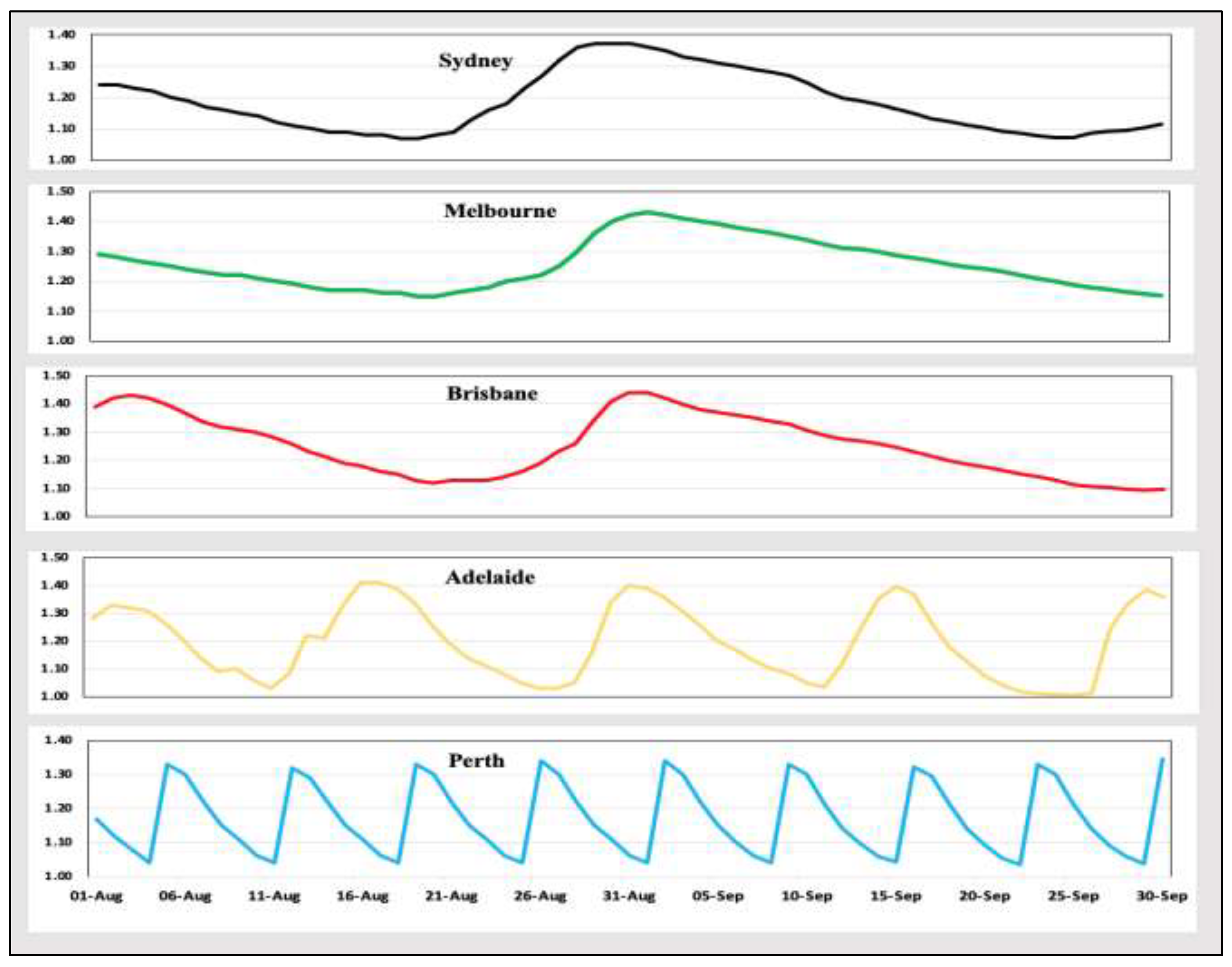
The existence of cycles has attracted significant attention to retail petrol markets. In cycles, prices rise quickly and decrease gradually over a short period of time [2]. In Australia, petrol price cycles exist in the five major metropolitan areas of Melbourne, Sydney, Adelaide, Brisbane, and Perth [3]. Figure 1 shows the average daily prices of unleaded petrol sourced from FuelPrice [4] and MotorMouth [5]: prices move up and down in consecutive and asymmetric cycles; price cycles vary in intensity and duration across cities. As reported by the ACCC, the duration of cycles in Melbourne, Sydney, Adelaide, and Brisbane varies and has increased unpredictably in recent years. Consequently, their cycles are unpredictable and have no specific peaks or troughs. Perth’s unique cycle has drawn the researchers’ attention to the retail petrol market in this metropolitan area and is the focus of this study.
The study contributes significantly to the literature on petrol markets. First, this study provides significant insights into the long-term pattern of price cycles. It applies a longer and more expansive dataset to examine Perth’s cycle characteristics over a long period (from 2003 to 2018). Second, based on the extensive and long-term dataset, we can investigate the impact of market changes on the petrol price cycles in Perth. The retail petrol market as well as macro- and micro-economic conditions may affect the petrol price cycles over time. Therefore, this paper aimed to examine the characteristics of Perth’s cycle over the past fifteen years. The research’s novelty lies in its attempt to answer the following question: Have there any changes in the characteristics of the petrol price cycle in Perth over the last 15 years?
The price cycle of retail petrol in Perth was estimated using a Markov regime-switching model. In light of the fact that daily petrol price cycles typically consist of two phases (price increase and price decrease), Markov regime-switching is the most appropriate model, which allows for the estimation of the distinct features of the two regimes. The petrol prices in Perth are very similar to the Edgeworth price cycle, so we used this theory to explain the pricing patterns in the retail petrol market in Perth. Edgeworth’s price cycle theory has been the most influential theory to explain price cycles, which is discussed in Section 2. The question raised here that we attempted to answer is as follows: Does the Edgeworth theory provide an accurate representation of price behaviors in Australia?
As reported by the ACCC [6], the duration of the cycles in Australian capital cities, excluding Perth, ranges from cycle to cycle and has lengthened in recent years. This study showed a weekly price cycle in Perth, which is frequent and predictable. Thus, it can be argued that the price legislation in WA has a significant role in facilitating a more regular cycle. A regular price cycle enables consumers to find the best days for purchasing petrol and save a substantial portion of their incomes. They can take advantage of the cycle by planning ahead and purchasing petrol at low prices. Decreasing prices last for six consecutive days in each weekly cycle in Perth. Thus, even if motorists need to fill up their tanks at more than once a week, Perth’s cycle gives motorists the opportunity to choose one of these cheap days, and they can save hundreds of dollars a year on fuel costs.
The rest of this paper is structured as follows. Section 2 provides a review of the theory and literature. A summary of the retail petrol market in Perth is presented in Section 3. The empirical framework and a short explanation about the data are given in Section 4 and Section 5, respectively. Section 6 contains the empirical results, and Section 7 includes our conclusions and the policy implications.
2. Background and Literature
The first part of this section explains the theoretical and analytical models, and the second part focuses on the empirical research on the retail petrol markets.
2.1. Edgeworth Price Cycle Theory
The cyclical pattern of petrol price is very similar in appearance to the Edgeworth cycle introduced by Maskin and Tirole [7]. The context of a dynamic, competitive, and asymmetric cycle goes back to Edgeworth [8], who argued that prices in a competitive market would not be stable based on the Bertrand model [9], and that they would change continually along a price cycle [10]. The seminal theory paper on Edgeworth cycles was by Maskin and Tirole, who provided game-theoretical foundations for the Edgeworth theory. Later extensions on the Edgeworth theory were undertaken by Eckert [11] and Noel [12]. They considered a dynamic price-setting game under the condition that two equal-sized firms sell homogeneous products under constant demand. They also assumed that firms were restricted to using Markov strategies, which means that one firm’s pricing decision depends on the pricing of another firm [13]. Their approach demonstrates the probability of two possible types of price setting under Markov equilibrium: the first illustrates the price stickiness over time, while the second shows asymmetric price cycles [14].
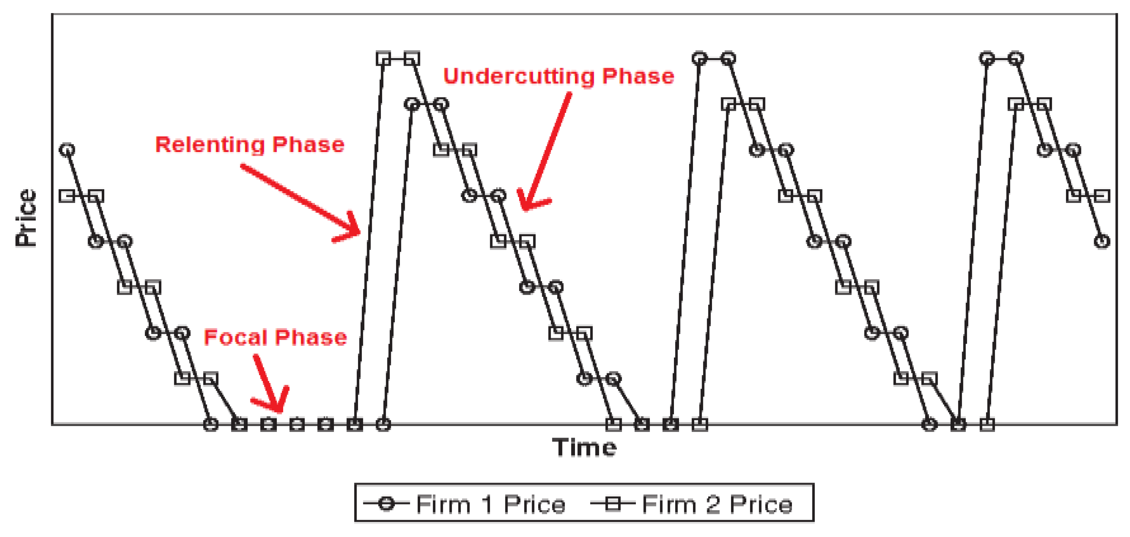
Maskin and Tirole assumed that a price cycle exists in a market with two firms that sell a homogeneous product. Figure 2 shows an example of the Edgeworth price cycle when two firms in a market sell a homogeneous product. In the Edgeworth cycle, firms consecutively undercut one another by offering goods at a lower price than their rivals to gain the market share until the price reaches marginal costs. At this point, one firm increases its price, and other firms follow it, and the undercutting phase starts again. Maskin and Tirole determined that firms with an Edgeworth price cycle follow three main predictions of the theory, which are as follows: (1) the reaction of firms is fast, but not simultaneous; (2) small-sized companies tend to lead in decreasing prices in the undercutting phase; and (3) large companies are more interested in being leaders in increasing prices in the relenting phase [10].
Retail petrol markets are similar to the market introduced by Maskin and Tirole in analyzing the Edgeworth cycle theory. Petrol is a relatively homogeneous product; there are different sized retailers in the petrol markets, and some specific markets are highly competitive, particularly in capital cities. Consequently, the petrol price cycles observed in the retail market around the world are very similar to the Edgeworth cycle. In these markets, a large number of small independent stations undercut their prices to gain a higher portion of the market and can persuade major petrol stations to follow them. When the price becomes very close or even equal to the marginal costs, the role of stations changes. One major station increases its price, and other stations follow it by increasing their prices. Therefore, both small retailers and large retailers are vital in creating a cyclical pattern in the retail petrol market.
It must be noted that the price cycle does not exist in less-competitive markets where there are only a few small retailers. Indeed, a small group of independent stations with low market power cannot gain a large enough fraction of the market through price competition and so cannot easily influence the price settings of major stations. Thus, a cyclical pattern is absent as no downward pressure on prices at major brand stations is exerted. When there are a number of small stations that are individually small but together form a large share of the market, cyclical patterns occur. Under these conditions, small stations can easily persuade major stations to follow them in undercutting [13,14,15]. Consequently, the price cycle likely exists in highly competitive markets characterized by many small independent retailers.
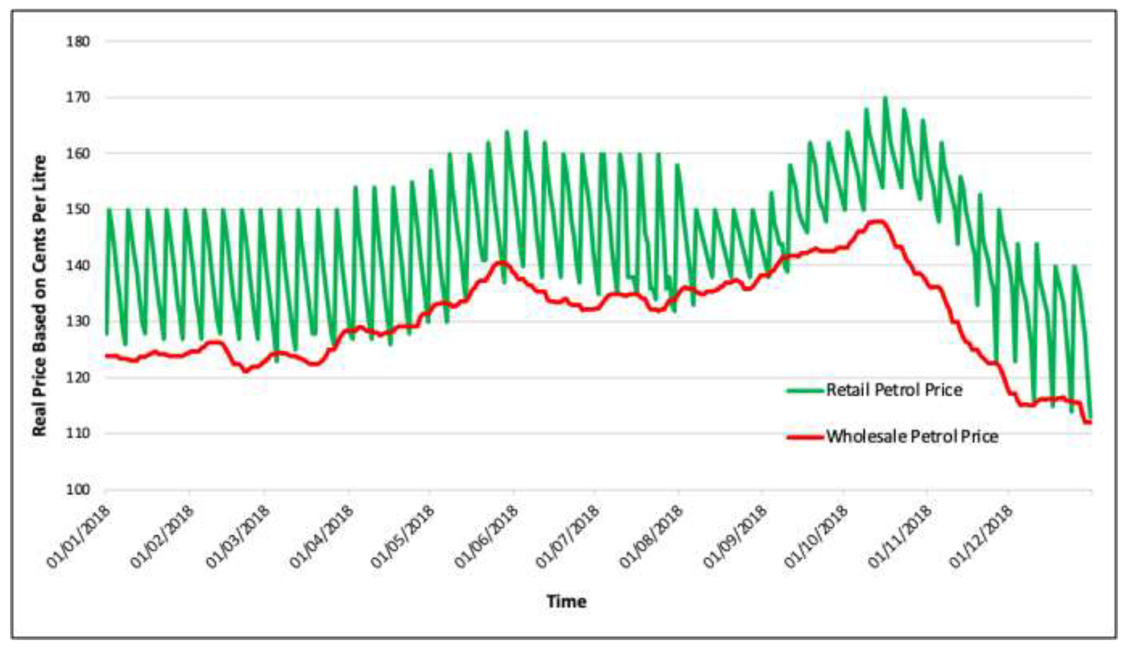
Cycles have been observed mainly in the capital and large cities of the U.S., Canada, and some European countries. Retail petrol prices move in cyclical patterns in Melbourne, Sydney, Adelaide, Brisbane, and Perth, the Australian capital cities. Figure 3 demonstrates an asymmetric pattern of petrol prices in the real market of Perth. This graph contains the time-series pattern of the average wholesale and retail petrol prices in Perth for the year 2018. As shown, the wholesale pattern is more stable and does not have daily fluctuations. In contrast, the retail price moves cyclically like the Edgeworth price cycle. Retail prices are completely linked to wholesale prices over the long-term, but their daily movements are not.
2.2. Markov Regime-Switching Model
A Markov switching model is widely used for analyzing the dynamics of the financial and economic variables. In recent years, the research on price cycles has been dominated by Markov models [17,18,19]. Economic variables (mainly macroeconomic and financial variables) often exhibit cyclical patterns: for instance, prices behave quite differently during Edgeworth cycles in low and high growth stages. Markov models are useful for analyzing such cycles. They use state variables for different regimes, and parameters move discretely between a fixed number of regimes. This part of the paper explains the features of the Markov regime-switching model using a simple model. A simple Markov switching panel model with M (m = 1, …, M) features, specification for i (i = 1, …, N) individuals, at time t (t = 1, …, T) for the variable yit is given by Equation (1) [20,21]:
Let:
where Xi is a matrix, and ji, yi, and εi are the column vector. Equation (1) can be rewritten as follows:
In a more compact version:
D is a matrix, and is matrix of intercepts so that each individual has a different intercept term. Equation (3) is called the least squares dummy variable (LSDV) model. The regime-switching mechanism is added to the LSDV model to make the MS-LSDV model as follows:
Consider that st is the unobserved state variable, X is the explanatory variables, and εt is a normally distributed error term with mean zero and variance σ2. Equation (4) illustrates the dynamic structures of variable Y according to its state at different levels. In these conditions, we can measure the behavior of the dependent variable in different states. Moreover, suppose that st follows a first-order Markov chain with the following transition matrix:
In Equation (5), P demonstrates the probability of switching between states and pij (i = 0 and j = 1) shows the switching probabilities of the state i at time t − 1 to state j at time t. Markov models are not restricted to two regimes, although two-regime switching models are prevalent [22,23,24].
This research applied the regime-switching model to analyze the price cycle, following Noel [13] and de Roos and Katayama [25]. Even though there are different methodologies such as time-series and threshold models to estimate the price patterns, this method offers significant advantages. In the first place, the model can be used to explain the time-series behavior of financial and economic variables that exhibit distinct patterns over time. Second, according to the Edgeworth theory, the undercutting and relenting cycles are expected to be asymmetric with different characteristics. Thus, the Markov method allows us to describe the cycle characteristics during the undercutting and relenting phases separately. Third, this model enables us to obtain a robust delineation of the specifications of the Edgeworth cycles in the retail petrol market such as cycle duration and cycle amplitude [25].
2.3. Related Literature
Edgeworth has been the leading theory for explaining the cyclical pattern in retail petrol markets. Maskin and Tirole [7] assumed that a price cycle exists in a market with two firms that sell a homogeneous product while the demand and marginal costs are constant. However, not all of these assumptions apply to retail petrol markets [26]. The Maskin model was developed by Noel [12] by studying a triopoly market with differentiated products when the capacity constraints, marginal costs, and elasticities are not too strong. Another limitation related to Maskin’s analysis is that they considered a constant competitive market with two equal firms. This means that when prices are the same, the market is divided into two similar groups with similar sales. However, a constant competitive environment with just two firms, in reality, cannot exist. In another extension, Eckert [27] adjusted this theoretical model by considering two unequal-sized firms in the retail petrol market in Canada. He found that in the market with two equal-sized firms, the market is divided into two firms based on their size when the prices are the same. Indeed, a more prominent firm has a higher share of the market. Alternatively, when prices are not equal, a firm with a lower price can gain the market share. Consequently, the smaller the firm, the higher the incentive to undercut. He concluded that only the Edgeworth price cycle could exist in markets with different firm sizes [13]. According to the Edgeworth theory and its developments, the size of the firm influences the shape of the price cycle.
The majority of scholars have analyzed the existence of the Edgeworth cycle in the retail petrol market using low or high-frequency datasets. Some of these studies are mentioned in Table 1.
Regarding the importance of petrol in the residential and commercial sectors and concern about its prices, there is an increasing number of governmental and organizational reports about petrol prices in Australia. For example, the ACCC is an independent Commonwealth statutory authority to observe and monitor prices. Several aspects of the petroleum market have been studied in Australia, and some studies have been devoted to examining the petrol price dynamics in the retail market (refer to Table 1).
Wang [37] examined the leadership pattern in the retail petrol market in Perth from July 2000 to October 2003. By comparing the pricing patterns before and after the 24 h rule, he found that BP acted as the price leader before the rule was implemented, while stations used a variety of strategies to determine price leadership after regulation. He only examined the leadership patterns in the retail petrol market for a short time and did not consider the cycle characteristics. The study by de Roos and Katayama [25] is closely related to this study, which analyzed a quantitative characterization of the petrol price cycle in Perth for 2003. However, that study had some limitations. The model examined the cycle for one year so that the effects of market fluctuations would not be considered. In addition, the study covered a period of 15 years, so there have been numerous changes in the market that may have affected the characteristics of the cycles. For example, some brands have withdrawn from direct retailing such as Ampol, whereas new brands such as 7-Eleven have entered the market. Additionally, the number of brands decreased from 2003 to 2018 (there were 19 brands in 2003, while at present, there are 16 brands in the retail petrol market in Perth). As a result, Puma, United, Vibe, Woolworth, 7-Eleven, and Woolworth-related stations have increased, whereas Gull, Wesco, and Peak-owned stations have decreased. Given the changes in the market and micro-and macro-economic conditions over the past few years, it is necessary to discover whether there have been any changes in the characteristics of the petrol price cycle.
This study is thus motivated to use a more extended dataset of prices (2003–2018) to capture market changes in the model and examine the effects of long-term market variations on the petrol price cycle. It seeks to provide valuable and up-to-date results over and above the previous studies. This study’s novel aspect addresses the following question: How has the petrol price cycle changed over the past fifteen years, despite the changes in both the macro and micro situations of the economy and the market? The purpose of this study is to extend previous studies by examining the role of days in the retail price cycles for the long-term from 2003 to 2018.
3. The Retail Petrol Market in Perth
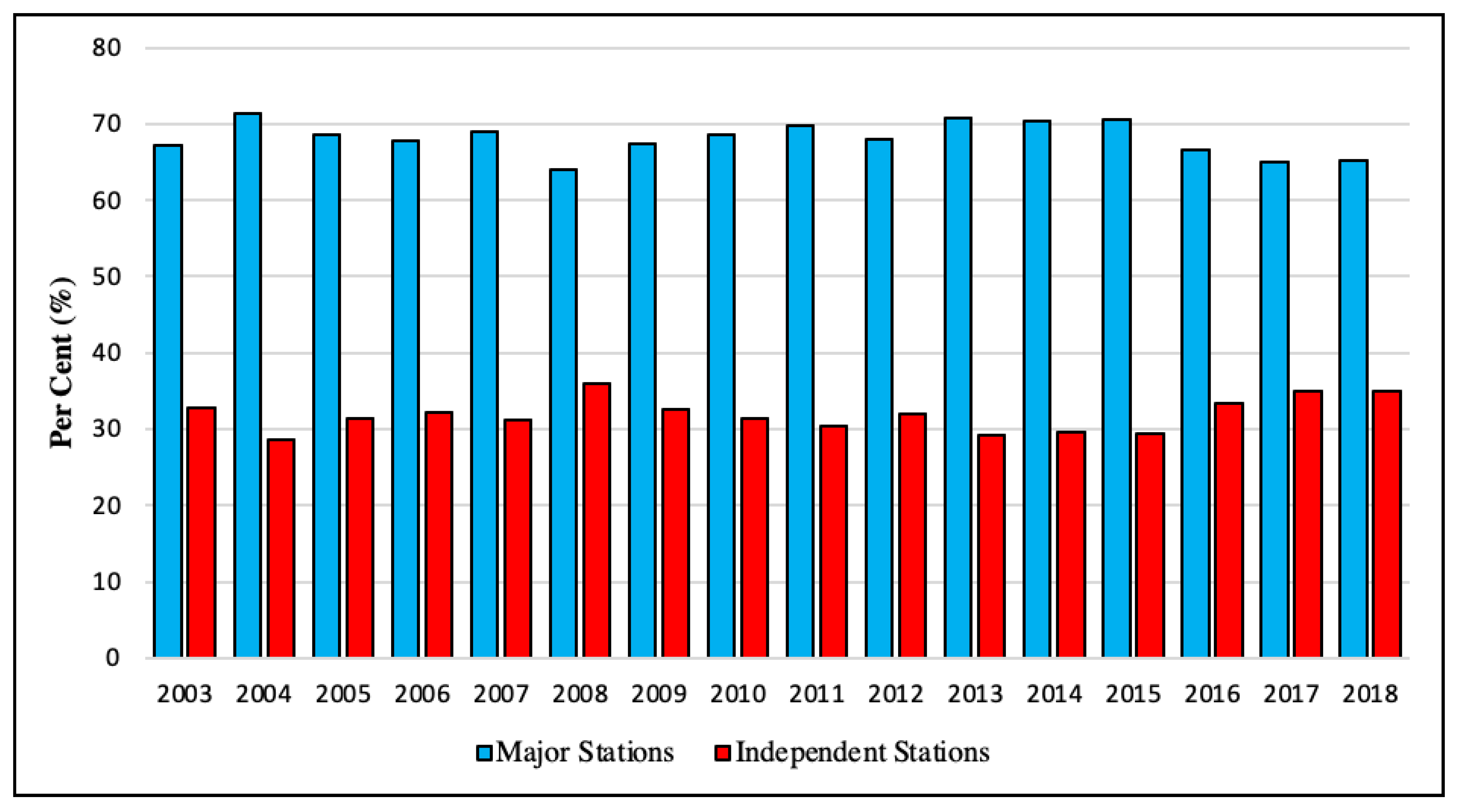
Perth is one of the most isolated capital cities globally; Adelaide, at a 2100 km distance, is the nearest capital city to Perth [62]. Because it is too far from refineries in other states, petroleum products in WA are almost exclusively supplied by the Kwinana (BP) refinery owned by the BP oil company located in WA. Furthermore, Perth differs from other capital cities due to its price legislation. There are 634 stations in WA, while more than half (369) exist in Perth. The Australian retail market has two types of stations: major stations and independent stations. The majors are owned by refiner-wholesaler oil companies including BP, Shell, Caltex, and Mobil, and the two major supermarket chains, Coles and Woolworths. Independents range from large chains such as Puma and United to small ones such as Wesco. Figure 4 shows the market share of the two groups of stations in Perth: the market share of independent stations has been around 30%, which is significant.
4. Empirical Framework
This study applied a Markov switching-regression model to estimate the petrol price dynamics. It defines three separate regimes in the framework of the Markov model as follows:
- The undercutting phase (U) illustrates the decrease in petrol prices.
- The relenting phase (R) corresponds to a sharp rise in price.
- A non-cycling or focal regime (F), that is, the period when the price is stable. There are two sub-regimes in the focal regime:
- ◦
- Cost-based pricing (sub-regime “C”); when there are no specific regimes, retail prices follow the wholesale prices.
- ◦
- Price stickiness (sub-regime “S”); when the prices are stable outside cycles.
This research thus examined the pricing behavior using a three-regime Markov model.
4.1. Model for Undercutting and Relenting Regimes
The relenting or the undercutting regimes are determined as follows in Equation (6):
where:
In Equation (6), RETAILst is the retail petrol price of station s at time t; ΔRETAILst is the difference between the retail petrol price for station s at times t and (t − 1) and Xsti is a vector of explanatory variables; αi is the expected daily price change considering explanatory variables (Xsti) in each regime. Therefore, αR shows the daily price change in the relenting phase and αU likewise defines the undercutting phase. The error term, εsti is assumed to follow the normal distribution with mean zero and variance σi2:
4.2. Model for the Focal Regime
Equation (7) presents the focal regime (F) when a station does not change its prices:
XstF is an explanatory variable including both constant-term and wholesale prices. The error term, εsti, is assumed to follow the normal distribution with mean zero and variance σi2. In the model of focal regime (non-cycling regime), it is anticipated that retail prices follow wholesale prices. Hence the TGP (the wholesale price) is included in XstF in the model (7). Moreover, γsti in Equation (8) shows the probability of price stickiness in the focal regime. The probability of the sticky price of sub-regime S, conditional on i = F, U, by the logit form, is given by:
In Equation (8), γsti indicates the probability that a station does not change its prices within the undercutting and focal regime (it is anticipated that the price increase occurs in a single time [13]; thus, we did not consider sticky prices within the relenting regimes). The indicator Jst is equal to C (Cost-based sub-regime) and S (sticky pricing sub-regime) when the market is in the focal or undercutting phase. Vsti is a () vector of explanatory variables of station s at time t, and ζ is a () vector of parameters.
4.3. The Switching Probability
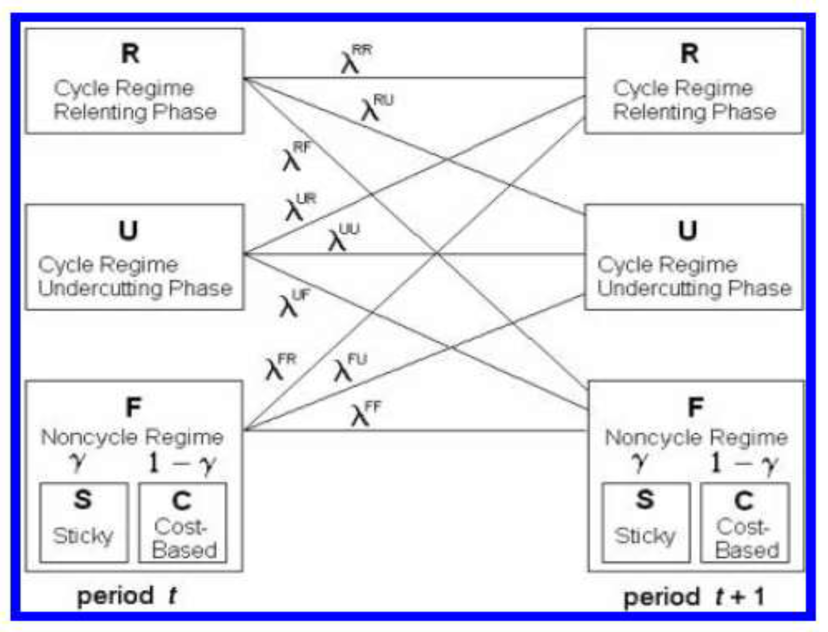
In the Edgeworth cycle, prices move between relenting, undercutting, and focal regimes. Considering the method introduced by Hamilton [24], this study estimated the switching probability between phases in the price cycle using matrix P:
where p21 defines the switching probability of regime 2 at time t − 1 to regime 1 at time t. The probability that a station switches from regime i in period (t − 1) to regime j in period t is given by:
where:
Ist is utilized as an indicator function equivalent to R, U, and F when station s, at time t, is in the phase of the relenting, undercutting, or the focal regime, respectively. Wist is a vector of explanatory variables, which influences switching from regime i, and θij is a vector of parameters and λst is a switching matrix [13]:
In Equation (12), λstRU shows the switching probability from the relenting to undercutting phase. Figure 5 shows nine switching probabilities of the Edgeworth cycle. Each large box depicts the undercutting, relenting, and focal regimes and the small boxes show the sub-regimes (cost-based or sticky prices). The switching probability out of regime i in time (t − 1) into regime j in time t, is presented by λij. Additionally, shows the probability of sticky prices conditional on regime i. The parameters βi, θi, ζi, and σi for each specification are estimated by the maximum likelihood.
4.4. Cycle Characteristics
According to the Edgeworth theory, and following the empirical study undertaken by Noel [13], the main characteristics of cycles were found by combining the switching probabilities and estimated parameters using a Markov model. After confirming the existence of the Edgeworth price cycle in petrol pricing dynamics, determining the characteristics of cycles is essential. The critical question is how long the relenting and undercutting phases last.
Durations of Cycle/Regime: As described earlier, λii shows the probability of stations remaining in regime i from period t − 1 to period t. In the next stage, I uses this index to find the duration of the regimes and cycles:
Cycle Amplitude: As explained above, αi is the average daily price changes during the relenting and undercutting regimes and γi is the probability of sticky prices in the undercutting phase. These indicators are applied to find the cycle amplitude as follows:
4.5. Description of the Empirical Model
According to the Edgeworth theory, several implementations will be tested from Equations (6) to (15) to find the price patterns of major and independent stations. This section describes the three specifications used in this study to describe the retail petrol price cycles.
4.5.1. Within-Regime Estimation
At the first stage, the basic characteristics of the retail petrol price cycle are examined. It is assumed that the expected price change in each regime (αi = E(ΔRETAILst|Xsti), i = R, U), the switching probabilities (λstij), and the probability of price stickiness are stable. In this specification, the constant term (a vector of ones) and the dummy variables for the type of stations (independent and branded) will be included in XR and XU as explanatory variables (Xsti) in Equation (6) to model the undercutting and relenting phases as follows:
The focal regimes are estimated through Equation (7) considering the constant term and the wholesale petrol price (TGP) as the explanatory variables (XstF) as follows:
The probability of price stickiness during the undercutting and the focal regimes will be estimated by Equation (8). In this specification, VU and VF are explanatory variables for these regimes and contain the constant term.
The switching probability between regimes is calculated by Equation (10) with Wi as the explanatory variable for all three regimes, which are only the constant term (a vector of ones) and dummies for the type of station.
4.5.2. The Effect of Position of Stations on the Petrol Price Cycle
Maskin and Tirole provided the predictions of behaviors of how minor and major companies behave during Edgeworth cycles. These main predictions are:
- (1)
- The reactions of firms are fast but not simultaneous.
- (2)
- Small-size companies tend to be the leaders in decreasing prices.
- (3)
- Large-size companies tend to be the leaders in increasing prices [50].
Following Noel [13], we considered two variables to test the behavioral predictions according to the cycle position and role of stations in the petrol price cycle: POSITION and FOLLOW. These variables will be included in the X, W, and V information.
The POSITION variable is applied as an indicator to display the location of stations in the cycles. Wholesalers sell petrol to retailers at the terminal gate price (TGP). With decreasing costs in the undercutting phase, stations approach the bottom of their cycles, retail prices become closer to the wholesale prices, and the retailers’ profit margins decline. Under these conditions, the switching probability from the undercutting to the relenting phase is expected to increase. We used the difference between the lagged retail petrol price and the wholesale price for each station as a proxy of the station’s positions:
BP, Caltex, Mobil, Puma and Viva are five brands of wholesalers in WA, which have six different locations. We matched the wholesale prices to the stations based on the distance and brand, for example, it was assumed that Caltex stations purchase petrol from the nearest Caltex wholesalers. It is expected that the position of the stations influences their price dynamics and the switching probability in cycles. When a station approaches the bottom of the cycle, it is more likely that the switching probability from the undercutting to the relenting term increases. In this section, the POSITION variable is added to the explanatory variables (XR, XU, VU, and WU) in Equations (6), (8), and (10). The POSITION variable is applied to show the effect of a station’s position on the expected price changes (αR and αU), the switching probabilities in the undercutting phase, and the probability of price stickiness in the undercutting phase (γU). Therefore, in the second estimate, XR, XU, and VU will contain the constant term, the dummy variables for the station type, and the POSITION variables.
The focal regimes can be estimated through Equation (7) by considering the constant term and the wholesale petrol price (TGP) as the explanatory variables (XstF) in this equation:
The probability of price stickiness during the undercutting and the focal regimes is estimated by Equation (8). In this specification, VU contains the constant term and the POSITION variables, and VF contains only the constant term. Moreover, in Equation (10), both WR and WF contain the constant term (a vector of ones) and dummies for the type of station, and WU includes the constant term, dummies for the type of station, and the POSITION variable. It is less likely that two sequential relenting phases occur during the cycles. Therefore, POSITION is not considered in WR (λRR ~ 0).
4.5.3. The Role of Stations in the Price Cycle
According to the Edgeworth price cycle theory, small firms tend to be pioneers in price decreasing, and large firms tend to initiate new rounds of the relenting phases. The FOLLOW dummy variable will then be added in the equations to learn how major and independent stations behave differently based on their roles as followers and leaders. To calculate this variable, the method of Noel [13] will be implemented. FOLLOW has two values, 0 and 1. FOLLOWSt takes the value of one (1) at time t for station S, when some other station has already increased their prices within the last six days by at least 6 cents (following de Roos and Katayama [25], so we considered 6 cents per liter as the minimum amount of price rise in the relenting phase), but station S still has not increased its price. FOLLOW takes zero (0) when Station S at time t has already raised its price.
There were 125 stations in the study sample, and it is complex to evaluate a calculation by considering the effect of all 124 stations on one station. It is also less likely that the price of a specific station connects to prices of all the other stations regardless of their location. As a result, we assumed that FOLLOW is considered 1 when a station has not started its relenting phase, while others in the radius of 5 km have commenced that phase (the distance between stations ranges from 0.006 km to 95 km). The FOLLOW indicator is added as an explanatory variable (XR and WU) in Equations (6) and (10) as follows:
The probability of price stickiness during the undercutting and focal phases will be estimated by Equation (8). In this specification, as explanatory variables for these regimes, VU and VF contain the constant term and dummies for the type of station. Moreover, Wi in the switching probability model for both focal and relenting regimes contains only the constant term and dummies for the type of station. Furthermore, we wished to test the branded stations’ power for starting the relenting phase. Thus, the FOLLOW dummy variable was added to the switching probability model for the undercutting regime (WU) to understand the role of stations as followers or leaders in the price cycle.
5. Data
Petrol prices were sourced from FuelWatch website (www.fuelwatch.wa.gov.au, accessed on January 2019), which is operated by the Department of Consumer and Employment Protection. The study focused solely on the retail petrol market in Perth because of its unique legislation. The dataset contained the daily prices of unleaded petrol (ULP) for each station in Perth from 1 January 2003 to 31 December 2018. It must be noted that, unlike petrol, diesel and LPG prices do not move in a cycle, and their prices remain relatively stable [63]. Different fuel types are supplied by different individual stations including Ethanol 94 (E10), Unleaded 91, Ethanol 105 (E85), Premium 95, Premium 98, Biodiesel 20, CNG/NGV, and EV. In Australia, ULP is the most widely used type of petroleum product, which is why it was the focus of this study. ULP prices are defined based on cents per liter (CPL) in real terms.
Each station’s brand and location were included in the dataset. There was a variety of major brands, supermarket chains, and independents in the dataset. This study applied a unique dataset of daily retail petrol prices for 125 stations in the Perth metropolitan area (including 86 major and 39 independent stations). It must be noted that during the sample period, some stations entered the market, while several stations exited it. There are more than 300 stations in Perth; 125 stations had complete price information from 2003 until 2018. Table 2 illustrates the descriptive statistics of the daily petrol prices with 707,083 observations from 1 January 2003 to 31 December 2018. The average petrol prices varied across brands during the sample period, ranging from 124.44 CPL for Peak stations to 133.79 CPL for Shell. As shown, most independents such as Peak and Better Choice had cheaper petrol than the major retailers such as Shell and Coles.
The study applied wholesale petrol prices (terminal gate prices (TGP)) from 1 January 2003 to 31 December 2018. The information on TGPs enabled us to identify the characteristics of the retail petrol price cycle when stations are in the focal regime and retail price is only dependent on the wholesale price. Five terminal operators in Perth supply all retail stations (BP, Caltex, Shell, Mobil, and Puma). We matched the retailers with wholesalers based on distance and brand: for instance, this assumes that BP stations purchase petrol from BP wholesalers, while Coles stations buy petrol from the nearest Shell wholesalers. Hence, GIS software was applied to find the geographical locations and distances.
6. Empirical Results
6.1. Basic Characteristics of the Petrol Price Cycle
We determined the cycle’s basic characteristics using Equations (6) to (18), which are presented in Table 3. In this specification, the constant term and dummies for the type of station (independent, major) are included in Wi, XR, XU, and XF consists of both the constant term and TGPs.
The probability of price stickiness (ΔP = 0|U) for major stations in the undercutting phase is zero, and for independents, it is 0.002, which is insignificantly different from zero. This means that stations change their prices every day, which is in contrast with the prediction by Maskin and Tirole. The reaction of firms to price changes is fast but not simultaneous; firms can observe their competitors’ prices before determining and deciding their next prices. However, this condition does not exist in Perth’s retail petrol price cycles because of the WA pricing legislation. Thus, stations must set their prices for the following day before 2:00 p.m., and then they can see their rivals’ prices.
The daily average price rise in the relenting phase is denoted by αR. According to Table 3, major stations raise their prices by 14.10 CPL on average in one day of relenting, while independent stations raise their prices by 13.4 CPL. Moreover, the daily average price decrease in the undercutting phase is illustrated by αU, and the amount was −2.25 and −1.92 for the major stations and independents, respectively. In other words, stations reduced their prices by 2.25 or 1.92 CPL on average every day during the undercutting phase. Based on these results, independent stations are less likely to increase their prices in the relenting phase than branded stations, and they are more likely to begin the undercutting phase by lowering prices. It can be argued that the existence of independent stations in the retail petrol market in Perth can exert a downward pressure on petrol prices.
The switching probability from one relenting phase to another relenting phase (λRR) was very small and almost close to zero for both types of stations. This result is in line with the prediction of Maskin and Tirole [7] that the price increase occurs in just one step. The finding shows that the probability of two consecutive relenting phases in cycles is rare. Moreover, λRU is the switching probability from the relenting to undercutting phase, and as shown in Table 3, this probability was significant, with 97% for the majors and 92% for the independents. This implies that the process of raising prices lasts only one day and then, in the next stage, the two groups of stations decrease their prices with the probability of 97% and 92%. Additionally, λUU represents the probability of switching from one undercutting phase to another undercutting phase. The λUU was 84% for majors and 82% for independents. However, there was a low probability for switching from the undercutting to the relenting phase for both kinds of stations (λMajUR = 0.12 and λIndUR = 0.09). All of the results showed that the undercutting phase lasted for more than one day in sequential steps.
The coefficients of the probability of price stickiness (ΔP = 0|F) in the focal phase for both branded stations and independents were statistically significant (Pr(ΔP = 0|F)Maj = 0.70 and (Pr(ΔP = 0|F)Ind = 0.87). This indicates that, under the focal regime, approximately 70% of the days for major stations and 87% of the days for independent stations were stable, and no price changes occurred on those days. Wholesale price increases or decreases were, however, passed on entirely to the retail petrol prices.
6.2. Effect of the Stations’ Positions on the Price Cycle
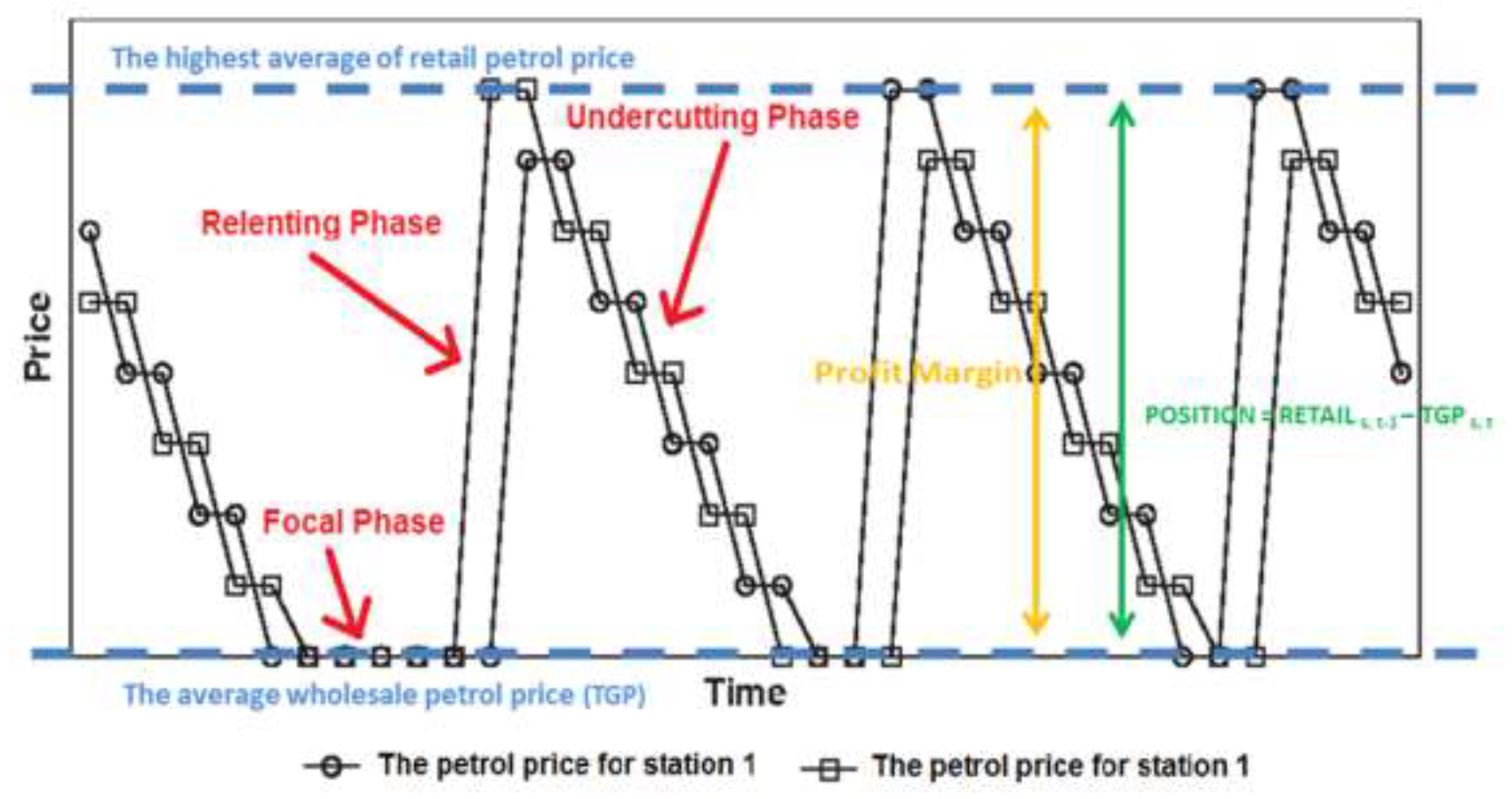
As mentioned earlier, stations purchase petrol at the terminal gate price (TGP) from wholesalers. Accordingly, TGP is the minimum price for stations to provide petrol to their customers. Retail prices are higher than wholesale because several extra costs such as operating, and distribution costs are added to the TGP. Consequently, when prices fall in the undercutting phases, the retail price approaches the wholesale price, and the profit margin drops. Since stations will wish to increase their profits, it is expected that switching from undercutting to relenting will be more likely at this point. The POSITION variable is used to examine the effect of station position in the cycle (Figure 6). This variable is the difference between the lagged retail price and the current wholesale price for each station (POSITION = RETAILs, t−1 – TGPs,t). This section examines the cycle characteristics by considering the POSITION variable. Table 4 presents the results of Equations (6) to (12) as well as (20) and (21).
In Table 4, αR presents the daily average price rise in the relenting phase. During this phase, the majors and independents raise their prices on average by 14.36 and 13.57 CPL per day, respectively. By controlling the POSITION variable, the size of the price rise is considerably larger for the independents as well as for the major stations. This may occur because stations are more sensitive to their positions. In cases where the retail price is equal to the wholesale price, the stations earn no profit and may even face losses due to additional operating costs. Under this condition, they tend to increase their price by a notable amount to meet their losses. Thus, the increased size of the price rise by considering the POSITION variable is reasonable.
In Table 4, “∂αR/∂POSITION” represents the amount of the price rise in the relenting phase by considering the stations’ positions in the cycles. There was a negative relationship between the magnitude of the price rise and the stations’ positions (∂αR/∂POSITIONMaj = −0.165; ∂αR/∂POSITIONInd = −1.14). This means that when the amount of the POSITION variable decreases at the bottom of cycles (or the profit margin decreases), stations tend to raise their prices to cover their losses, resulting in a lower profit. Additionally, “∂αU/∂POSITION” shows the average amount of the daily price decrease in the undercutting phases by considering the POSITION variable (∂αU/∂POSITIONMaj = −0.133, ∂αU/∂POSITIONInd = −0.01). This signifies that both the major and independent stations decrease their prices less sharply and wait upon a new round of the relenting phase at the bottom of the cycles.
The probability of price stickiness during the undercutting phase is displayed by γU, and “∂γU/∂POSITION” illustrates this probability with respect to the stations’ positions. The results in Table 4 demonstrate that major stations at the top of the cycle are more interested in holding petrol prices stable (∂Pr(ΔP = 0|U)/∂POSITION = 0.02), while independents tend to undercut their prices (∂Pr(ΔP = 0|U)/∂POSITION = −0.01). The role of the stations switches at the bottom of cycles. Major stations do more to decrease their prices, while independents prefer to hold their prices constant. The findings show that independents are more sensitive to their profit margins and, by decreasing the amount of these, they prefer not to reduce their prices.
The last three rows show the switching probability during the undercutting phase by considering the position of stations. The amount of λUR was −0.01 and −0.03 for the majors and independents, respectively. This means that by decreasing the margin, the switching probability from the undercutting to relenting phase rises. The findings illustrate that the POSITION variable in the cycle influences both the magnitude of the price changes and the regime transition dynamics.
6.3. The Role of Stations in the Petrol Price Cycle
This section examines the role of stations as leaders or followers using the FOLLOW variable. Table 5 represents the outcomes of Equations (6) to (12), and of Equations (22) and (23), when the FOLLOW variable is considered in the regression. According to the Edgeworth theory, large firms (major brands), as leaders, tend to initiate new relenting phases in cycles, and small firms (independent stations) tend to follow them. We considered the FOLLOW dummy variable to find the role of stations in the cycle. According to Noel [13], a follower is a station where the value of its FOLLOW dummy variable is 1. Under this condition, that station has not yet increased its price in the current cycle, but at least one other station within a 5 km radius has. The FOLLOW is zero when a station has already increased its price.
The average daily price rise (αR) was 14.52 CPL for majors and 13.42 CPL for the independents. The results show that the independents follow major stations in the relenting phase by lower price rises. Additionally, “∂αR/∂FOLLOW” shows the price growth in the relenting phase by controlling the FOLLOW variable. It shows that the majors, as followers, tend to raise their prices by 0.73 CPL less than the leaders. Indeed, by selling petrol at lower prices, followers can gain a higher market share and profit, while independent followers behave differently. The size of the price rise was 1.9 CPL more than for the independent leaders in relenting because independent followers are less interested in undercutting and prefer to keep their high prices. In WA, there are more major retailers than independents, and these retailers have a high market share. Despite the independents’ preference for higher prices, they do not have the power to influence the market in their favor. Therefore, they raise their prices higher than the leaders do to keep them in a relenting phase for the next day [25]. The pricing behavior can also be explained by the following factor. Independent stations sell petrol very cheaply and make very little profit at the bottom of the cycle. Consequently, when the relenting phase starts, they increase their prices more than the major stations in order to gain more profit.
The switching probabilities in the undercutting phase for the following stations are reported at Table 5 (∂Prλ/∂FOLLOW). As can be seen, the switching possibility from the undercutting to relenting phase for followers was significant. This shows that followers are more likely to move from the undercutting to the relenting phase once a cycle has commenced.
Table 6 illustrates the cycle characteristics by evaluating the effect of both the POSITION and FOLLOW indicators in a single specification. The results related to the average daily price rise, the average daily price drop, and the switching probabilities were similar to the estimated results presented in Table 2, Table 3 and Table 4.
The main characteristics of the cycles for both the major and independent stations are presented in Table 7. As illustrated, the duration of the relenting phase lasted a single day for both kinds of stations. Additionally, the undercutting period lasted approximately six days, with the average daily price decrease around 2 cents per day. Generally, petrol stations increase their prices only for one day and then decrease them sequentially for six consecutive days. Hence, there was a weekly cycle in the retail petrol market in Perth from 2003 to 2018. These results provide evidence for the Edgeworth theory that the cycle is extremely asymmetric and frequent. Previous studies have shown similar results in the retail petrol markets in Canada, the U.S., and Australia (e.g., Lewis [32] and Doyle et al. [38] in the U.S.; Noel [15] in Canada; and Wang [36,37] in Australia).
6.4. Peak and Trough Days
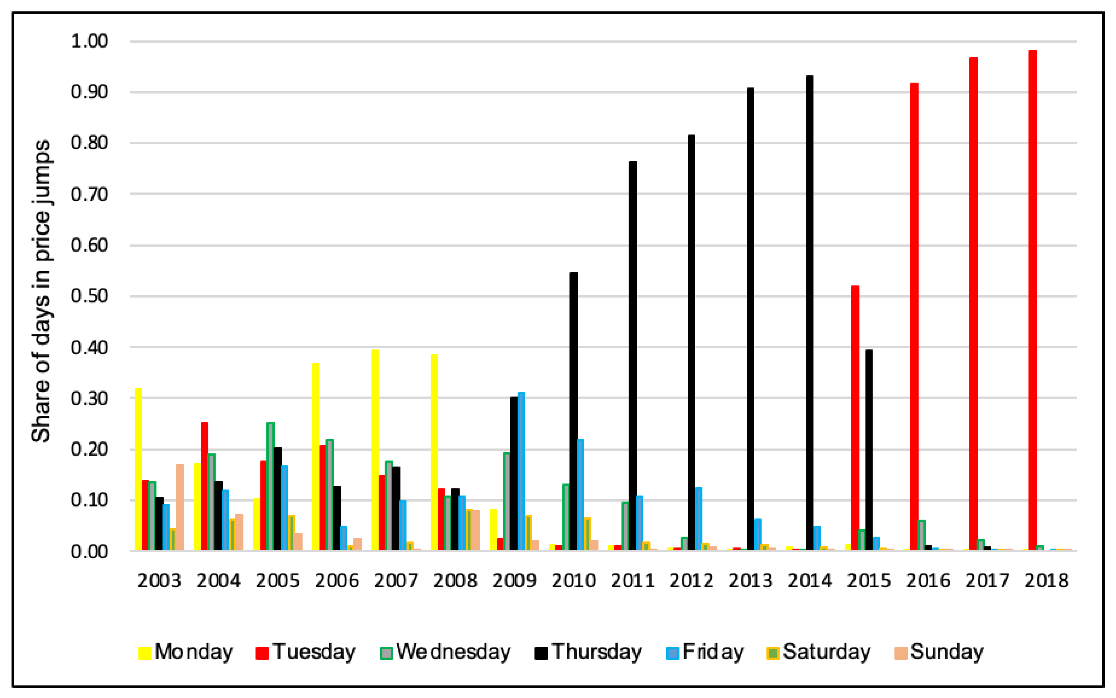
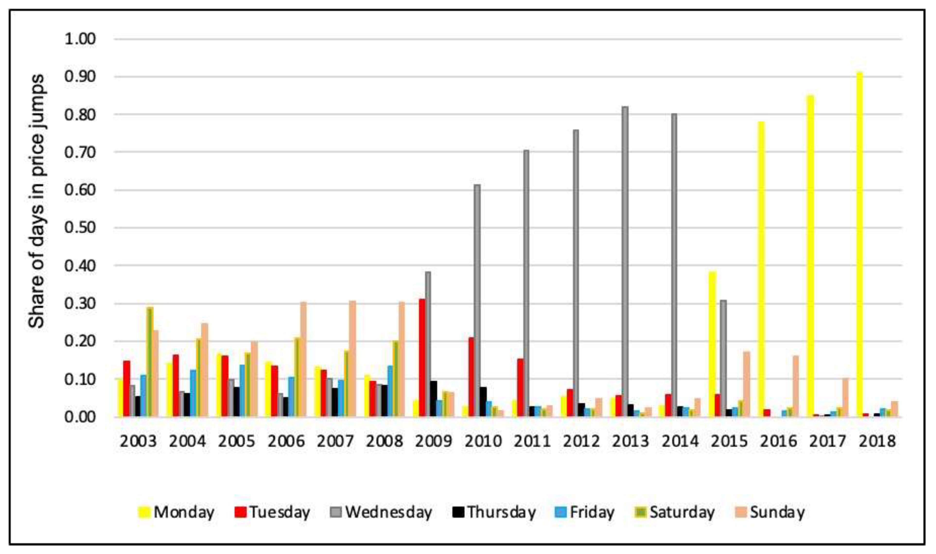
A series of tests were used to find the cheapest and the most expensive days of petrol from 2003 to 2018. Figure 7 and Figure 8 illustrate the share (%) of days engaging in price jumps and price undercuts, respectively. Table 8 and Table 9 present each day’s share as peak days or trough days during these years. During these years, the role of days changed several times.
In 2003, Monday was the most expensive day to buy petrol (32% of relenting phases happened on Monday), while Saturday (29%) was the cheapest day in Perth. Peak days in 2004 and 2005 were Tuesdays and Wednesdays. From 2006 to 2008, Mondays were the most expensive days for petrol two years in a row. The cheapest day was Saturday in 2003. From 2004 to 2008, Sunday was the lowest day for purchasing petrol for five consecutive years. However, the role of days was not significant, and there was no specific peak day or trough day in the cycle from 2003 to 2010. Since November 2010, when petrol stations raised their prices on Thursdays, the role of days has changed dramatically. For about five years (2010–2015), Perth experienced a frequent and predictable weekly cycle where Thursday was the most expensive day of the week, and Wednesday was the cheapest.
In 2015, the role of days changed again. In May–June 2015, the cycle was disrupted for two weeks. At the end of May (21 May), most Caltex stations abruptly broke the cycle pattern and ceased increasing their prices on Thursday (28 May). With effect from 2 June, Caltex stations established new peak and trough days in the cycle, where Tuesday was the most expensive day of the week, and Monday was the cheapest. After a few weeks, other brands followed Caltex’s lead by increasing their prices on Tuesdays. Therefore, from June 2015 to 2018, Monday was the cheapest day, and Tuesday was the peak day. The role of Monday as the cheapest day for buying petrol has been very significant in recent years. As shown in Table 9, Perth had 78% of trough days on Monday in 2016, and this reached 91% in 2018. The research shows that petrol prices have been more predictable since 2009. As a result, consumers can buy petrol at the lowest price on Monday and save a significant portion of their income in comparison to the years before 2009.
6.5. Investigation of Energy Markets Regarding Substitute Petrol by Clean Energy Source in the Future in Australia
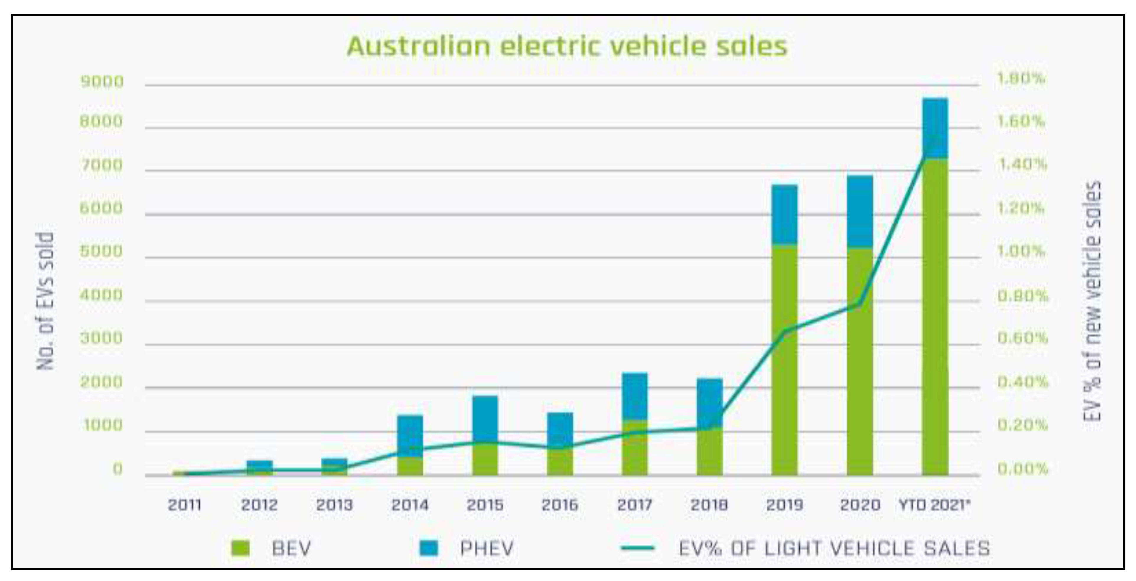
Although our energy supply is still heavily reliant on non-renewable fossil fuels such as coal, oil, and gas energy, but whether we want to or not, we need to change toward clean energy sources as soon as possible. Luckily, the transition to renewables and electrification, can not only be a driver for environmentally-friendly energy production and use but can reduce the dependency on fossil fuels [64]. In Australia, the government is struggling to develop hybrid cars as well as fully electric. Of course, over recent years, the renewable energy investment has increased significantly. Actually, a combination of factors including elevated electricity prices, government policy incentives, and declining costs of renewable generation technology is the main cause of this. Therefore, it means that dependence on petrol and producing it will be reduced year by year while EVs will develop [65]. On the other hand, the results of the research show that in terms of energy consumption (with the current electricity mix), battery electric vehicles (BEVs) in Australia perform better than other types. Based on the research, BEVs emit 40% less GHGs than the second-best, fuel cell EVs (FCEVs), in Australia [66].
Figure 9 [67] shows the electric vehicle sales in Australia from 2011 to 2021. As can be seen in this figure, from 2011 to 2021, Australia has experienced a dramatic growth in electric vehicle sales, showing that the interest of people in the utilization of EVs in recent years has increased. Therefore, can be said that petrol in future years cannot remain as the main fuel when EVs are developing.
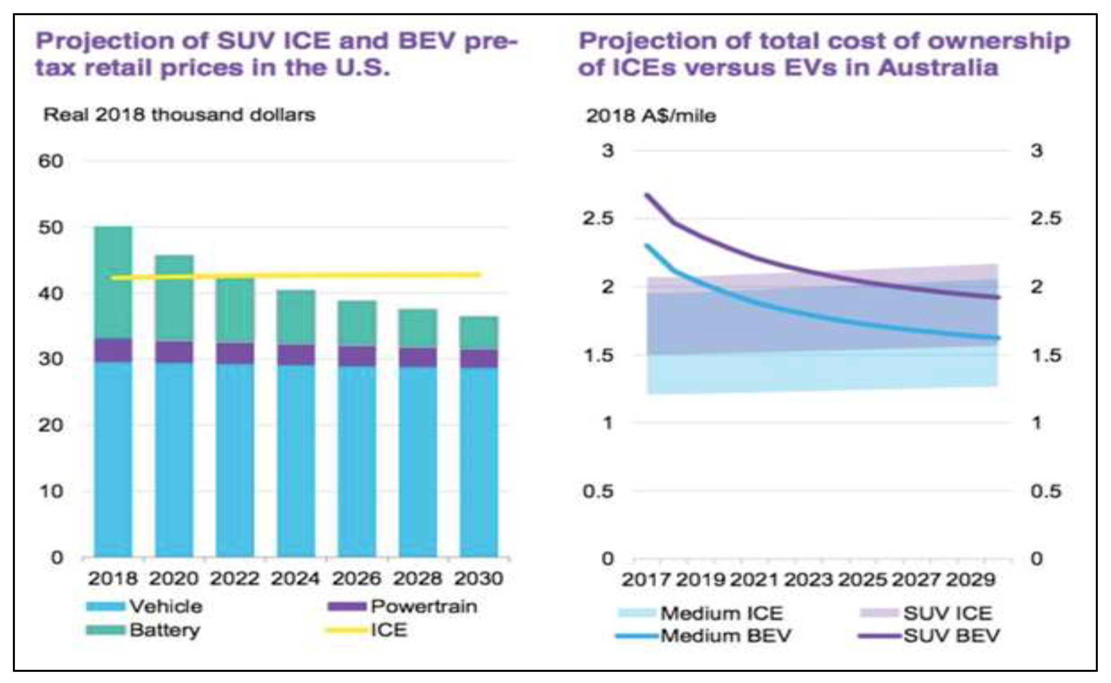
In addition, Figure 10 shows a projection between the U.S. and Australia until 2029. Indeed, this graph illustrates BNEF’s forecast for the total cost of ownership in Australia. It shows that it may be another few years before the popular SUV vehicle class reaches parity, but medium-sized battery electric vehicles could reach TCO parity in 2020. It also shows that Australia in the upcoming years will have dramatically grown in the use and development of EVs, and without a doubt, for this country, in order to achieve its goals of CO2 reduction, reducing the dependency on fossil fuels, especially for the reduction in petrol and petrol cars, is serious. In addition, BNEF predicts that by 2030, the average cost of a midsize battery electric vehicle from more than $50,000 in 2018 to near $37,000 will decline by 2030.
7. Conclusions and Policy Implications
The importance of providing energy for countries is increasing, and petrol is among the most important energy resources. This research analyzed the retail petrol price dynamics using a new and expanded dataset for the Perth metropolitan area from 2003 to 2018 in order to investigate this fossil fuel and eventually investigate the future consumption of petrol with clean energy in Australian markets. This study extends the findings of the previous literature through an investigation of cyclical patterns over a long period of time. In addition to analyzing the quantitative characteristics of petrol price cycles using the Markov regime-switching method, this study examined changes in Perth’s cycle characteristics from 2003 to 2018. The novel aspect of this study was in addressing the following question: Have there been any changes in the characteristics of the petrol price cycle in Perth in the last 15 years?
The findings show the existence of a weekly price cycle in the retail petrol market in Perth, which is similar to the Edgeworth price cycle. As with the Edgeworth cycle, the petrol price cycle is asymmetric and frequent. In this weekly cycle, prices move in two phases—undercutting and relenting. In the undercutting phase, stations frequently undercut one another by selling petrol at a lower price than their competitors to take the market share until the price reaches the marginal cost. At that point, the relenting phase starts. One station relents and raises its price, and others follow it by increasing their prices to a level less than the first station’s price increase, and then a new cycle starts again. Using the Edgeworth theory, we found that the major-branded stations as leaders had a higher likelihood of initiating a new cycle with increasing prices than the independent stations, while there was an inverse relationship between small stations as followers and the likelihood of initiating new rounds of the undercutting phases by lowering their prices. According to the prediction of the Edgeworth cycle, the reaction of firms to the price changes is fast but not simultaneous. Firms can observe their competitors’ prices before determining and deciding their own next prices. However, this condition does not exist in Perth’s price cycles because of the pricing legislation in WA. Therefore, it can be argued that the Edgeworth cycle can exist in markets with different pricing environments.
As stated earlier, a form of competition causes a cyclical price pattern in the retail petrol markets. Additionally, the existence of both branded stations and independents has an essential role in increasing competition and creating cycles. Therefore, changes in the market conditions can influence the level of competition, leading to changes in the price cycle. However, the findings of this study show that the micro- and macroeconomic changes in the retail petrol market in Perth did not significantly affect the petrol price cycle. The Edgeworth features of the cycle were constant from 2003 to 2018. Retail petrol prices in Perth have fluctuated on a frequent and asymmetrical basis since 2003. Prices increase sharply in one day and decrease gradually for six consecutive days in the cycle. Major stations are the leaders in price increase, and independent stations are the leaders in price undercutting. Hence, it can be argued that the Edgeworth features of the petrol price cycle in Perth have not been changed from 2003 to 2018.s
In addition, the paper examined the role of days in the price cycle. The results illustrate a remarkable change in the role. By 2009, there was no specific peak or trough day with significant frequency on the cycle, and thus there was no special predictable day for buying petrol. Since 2010, the petrol price cycle has become more predictable and consistent than in 2003. The peak day was Thursday, and the trough day was Wednesday, from 2010 to 2015. The role of days changed again in 2015. Since 2015, Tuesday has been the day with the highest price, while Monday is the cheapest. It can be argued that the role of days became more predictable in 2018 compared with 2003. According to the findings of this study, consumers could not rely on petrol price cycles to buy petrol in Perth until 2009, but today, the price cycle is predictable and more reliable.
The findings have positive implications for motorists and authorities. Although the price of petrol in the retail market cannot be predicted, motorists can find the best days to purchase petrol by understanding the price cycle. The results of this study provide motorists with comprehensive information about the price cycle in Perth, allowing them to choose the best days to buy fuel. We found that Monday has been the cheapest day to buy petrol since 2015, a significant time in which to assure drivers to rely on the cycle.
Motorists in central Australian cities are irritated by daily or intra-day price fluctuations [31]. This may be because authorities such as the ACCC, the media, and even fuel websites such as FuelWatch mostly publish reports about the peak days in the cycles. For instance, FuelWatch publishes reports on the ‘ULP price hike’ every week. Therefore, these reports have a negative impact on the consumers’ perceptions about the price cycle. However, it should be noted that the weekly cycle in Perth has a considerable positive impact on consumers. A regular cycle enables consumers to discover the best days for purchasing petrol and save a significant portion of their incomes. They can potentially take advantage of the cycle by planning ahead and purchasing petrol on days when prices are low. In Perth’s petrol price cycle, the process of price decrease takes six consecutive days (from Wednesday to Monday). Thus, even if motorists need to fill up their tanks more than once per week, Perth’s cycle gives them the opportunity to choose one of those cheap days and save hundreds of dollars annually on fuel. Therefore, Perth’s weekly pattern of petrol prices gives motorists an advantage over the other Australian States where the petrol price cycles are unpredictable and vary from two weeks to more than five weeks.
According to the ACCC [3], the duration of petrol price cycles in Sydney, Melbourne, Brisbane, and Adelaide ranges from cycle to cycle and has risen in recent years. This study shows the weekly price cycle in Perth, which is frequent and predictable, with Monday being the cheapest and Tuesday being the most expensive day. The main difference between the retail petrol market in Perth and markets in other cities is the 24 h rule in WA, which is unique. This legislation has a significant role in facilitating a more regular cycle and eradicating intra-day price fluctuations in this state. Motorists in Perth can easily follow the regular weekly price cycle with predictable peak and trough days. The duration of petrol price cycles in other Australian capital cities is not regular, which results in less predictable peak and trough days/times. Hence, consumers cannot easily determine the relatively cheaper times to buy petrol in other states. Therefore, Perth’s pricing regulations have resulted in stable petrol prices with predictable price cycles, allowing consumers to plan and reduce their concerns.
Although this regulation has led to a regular cycle that is advantageous to consumers in Perth, this pricing restriction may reduce the level of market competition in the long-run, leading to higher petrol prices. In order to prevent future price gouging, the retail petrol market in Perth needs to be monitored more by the authorities. In the end, it can also be added that although petrol cars and the price of petrol are important issues in Australia, Australia will reduce the consumption of petrol in the next few years because of the CO2 emissions that this fuel has, and replace petrol cars with EVs, although it needs more time.
Author Contributions
Conceptualization, A.G. and A.R.; methodology, A.G.; software, A.G.; validation, A.R.; formal analysis, A.G.; investigation, A.G. and A.R.; resources, A.G.; data curation, A.G. and A.R.; writing—original draft preparation, A.G.; writing—review and editing, A.R.; visualization, A.G. and A.R.; supervision, A.G.; project administration, A.G.; funding acquisition, A.R. All authors have read and agreed to the published version of the manuscript.
Funding
This research received no external funding.
Institutional Review Board Statement
Not applicable.
Informed Consent Statement
Not applicable.
Data Availability Statement
FuelWatch. 2019. Historic fuel prices; https://www.fuelwatch.wa.gov.au/retail/historic.
Conflicts of Interest
The authors declare no conflict of interest.
References
- FuelWatch. How FuelWatch Works; The Department of Mines, Industry Regulation and Safety: Perth, Australia, 2021. [Google Scholar]
- Byrne, D.P. Petrol price cycles. Aust. Econ. Rev. 2012, 45, 497–506. [Google Scholar] [CrossRef]
- Australian Competition and Consumer Commission. About Fuel Prices. 2021. Available online: https://www.accc.gov.au/consumers/petrol-diesel-lpg/about-fuel-prices (accessed on 3 May 2022).
- Fuel Price, Monitoring of Petrol Price. Available online: www.fuelprice.io (accessed on 3 May 2022).
- MotorMouth, Reports of the Average Petrol Prices. Available online: www.motormouth.com.au (accessed on 3 May 2022).
- Australian Competition and Consumer Commission. Petrol Price Cycles in Australia; ACCC: Canberra, Australia, 2021. [Google Scholar]
- Maskin, E.; Tirole, J. A Theory of Dynamic Oligopoly, II: Price Competition, Kinked Demand Curves, and Edgeworth Cycles. Econometrica 1988, 56, 571. [Google Scholar] [CrossRef] [Green Version]
- Cannan, E.; Edgeworth, F.Y. Papers Relating to Political Economy. Economica 1925, 332, 111–142. [Google Scholar] [CrossRef]
- Bertrand, J. Review of theorie mathematique de la richesse sociale et recherches sur les principes mathematiques de la Richesse. J. Des. Savants 1883, 67, 499–508. [Google Scholar] [CrossRef]
- Noel, M.D. Edgeworth Price Cycles. New Palgrave Dictionary of Economics; Palgrave Macmillan: London, UK, 2011. [Google Scholar] [CrossRef]
- Eckert, A. Retail price cycles and the presence of small firms. Int. J. Ind. Organ. 2003, 21, 151–170. [Google Scholar] [CrossRef]
- Noel, M.D. Edgeworth Price Cycles and Focal Prices: Computational Dynamic Markov Equilibria. J. Econ. Manag. Strat. 2008, 17, 345–377. [Google Scholar] [CrossRef]
- Noel, M.D. Edgeworth price cycles: Evidence from the Toronto retail gasoline market. J. Ind. Econ. 2007, 55, 69–92. [Google Scholar] [CrossRef]
- Noel, M.D. Edgeworth Price Cycles in Retail Gasoline Markets; Massachusetts Institute of Technology: Cambridge, MA, USA, 2002. [Google Scholar] [CrossRef] [Green Version]
- Noel, M.D. Edgeworth Price Cycles, Cost-Based Pricing, and Sticky Pricing in Retail Gasoline Markets. Rev. Econ. Stat. 2007, 89, 324–334. [Google Scholar] [CrossRef] [Green Version]
- Australian Institute of Petroleum (AIP). Available online: https://www.aip.com.au (accessed on 3 May 2022).
- Hou, C.; Nguyen, B.H. Understanding the US natural gas market: A Markov switching VAR approach. Energy Econ. 2018, 75, 42–53. [Google Scholar] [CrossRef]
- Boroumand, R.H.; Goutte, S.; Porcher, S.; Porcher, T. Asymmetric evidence of gasoline price responses in France: A Markov-switching approach. Econ. Model. 2016, 52, 467–476. [Google Scholar] [CrossRef]
- Balcilar, M.; Gupta, R.; Miller, S.M. Regime switching model of US crude oil and stock market prices: 1859 to 2013. Energy Econ. 2015, 49, 317–327. [Google Scholar] [CrossRef] [Green Version]
- Kim, C.-J.; Piger, J.; Startz, R. Estimation of Markov regime-switching regression models with endogenous switching. J. Econ. 2008, 143, 263–273. [Google Scholar] [CrossRef] [Green Version]
- Chen, S.-W. Measuring business cycle turning points in Japan with the Markov Switching Panel model. Math. Comput. Simul. 2007, 76, 263–270. [Google Scholar] [CrossRef]
- Cosslett, S.R.; Lee, L.-F. Serial correlation in latent discrete variable models. J. Econ. 1985, 27, 79–97. [Google Scholar] [CrossRef]
- Ellison, G. Theories of Cartel Stability and the Joint Executive Committee. RAND J. Econ. 1994, 25, 37. [Google Scholar] [CrossRef]
- Hamilton, J.D. Regime Switching Models. Macro Econometrics and Time Series Analysis; Springer: Berlin/Heidelberg, Germany, 2005; pp. 202–209. [Google Scholar] [CrossRef] [Green Version]
- De Roos, N.; Katayama, H. Gasoline Price Cycles Under Discrete Time Pricing. Econ. Rec. 2013, 89, 175–193. [Google Scholar] [CrossRef]
- Wlazlowski, S.; Giulietti, M.; Binner, J.; Milas, C. Price dynamics in European petroleum markets. Energy Econ. 2009, 31, 99–108. [Google Scholar] [CrossRef]
- Eckert, A. A Study of Canadian Gasoline Retail Prices; University of British Columbia: Vancouver, BC, Canada, 1999. [Google Scholar]
- Eckert, A. Retail price cycles and response asymmetry. Can. J. Econ. Rev. Can. D’économique 2002, 35, 52–77. [Google Scholar] [CrossRef]
- Eckert, A.; West, D. Retail Gasoline Price Cycles across Spatially Dispersed Gasoline Stations. J. Law Econ. 2004, 47, 245–273. [Google Scholar] [CrossRef]
- Eckert, A.; West, D.S. A tale of two cities: Price uniformity and price volatility in gasoline retailing. Ann. Reg. Sci. 2004, 38, 25–46. [Google Scholar] [CrossRef]
- Roarty, M.J.; Barber, S. Petrol Pricing in Australia: Issues and Trends; Department of the Parliamentary Library: Melbourne, Australia, 2004. [Google Scholar]
- Al-Gudhea, S.; Kenc, T.; Dibooglu, S. Do retail gasoline prices rise more readily than they fall? A threshold cointegration approach. J. Econ. Bus. 2007, 59, 560–574. [Google Scholar] [CrossRef]
- Li, Z. Modelling and forecasting the demand for automobile petrol in Australia, and its policy implications. In Proceedings of the 29th Conference of Australian Institutes of Transport Research (CAITR), Adelaide, Australia, 5–7 December 2007. [Google Scholar]
- Lewis, M. Price dispersion and competition with differentiated sellers. J. Ind. Econ. 2008, 56, 654–678. [Google Scholar] [CrossRef]
- Lewis, M.S. Temporary Wholesale Gasoline Price Spikes Have Long-Lasting Retail Effects: The Aftermath of Hurricane Rita. J. Law Econ. 2009, 52, 581–605. [Google Scholar] [CrossRef] [Green Version]
- Wang, Z. Station level gasoline demand in an Australian market with regular price cycles. Aust. J. Agric. Resour. Econ. 2009, 53, 467–483. [Google Scholar] [CrossRef]
- Wang, Z. (Mixed) Strategy in Oligopoly Pricing: Evidence from Gasoline Price Cycles Before and Under a Timing Regulation. J. Political Econ. 2009, 117, 987–1030. [Google Scholar] [CrossRef]
- Doyle, J.; Muehlegger, E.; Samphantharak, K. Edgeworth cycles revisited. Energy Econ. 2010, 32, 651–660. [Google Scholar] [CrossRef] [Green Version]
- Wills-Johnson, N.; Bloch, H. A simple spatial model for Edgeworth Cycles. Econ. Lett. 2010, 108, 334–336. [Google Scholar] [CrossRef]
- Bloch, H.; Wills-Johnson, N. The Shape and Frequency of Edgeworth Price Cycles in an Australian Retail Gasoline Market. SSRN 1558747. 2010. Available online: https://0-doi-org.brum.beds.ac.uk/10.2139/ssrn.1558747 (accessed on 3 May 2022). [CrossRef]
- De Roos, N. Do Firms Play Markov Strategies? SSRN 1597064. 2010. Available online: https://0-doi-org.brum.beds.ac.uk/10.2139/ssrn.1597064 (accessed on 3 May 2022). [CrossRef]
- Anderson, E. A new model for cycles in retail petrol prices. Eur. J. Oper. Res. 2011, 210, 436–447. [Google Scholar] [CrossRef]
- Lewis, M. Price leadership and coordination in retail gasoline markets with price cycles. Int. J. Ind. Organ. 2012, 30, 342–351. [Google Scholar] [CrossRef]
- Zimmerman, P.R.; Yun, J.M.; Taylor, C.T. Edgeworth Price Cycles in Gasoline: Evidence from the United States. Rev. Ind. Organ. 2013, 42, 297–320. [Google Scholar] [CrossRef]
- Valadkhani, A. Do petrol prices rise faster than they fall when the market shows significant disequilibria? Energy Econ. 2013, 39, 66–80. [Google Scholar] [CrossRef]
- Valadkhani, A. Seasonal patterns in daily prices of unleaded petrol across Australia. Energy Policy 2013, 56, 720–731. [Google Scholar] [CrossRef]
- Valadkhani, A.; Babacan, A. Modelling how much extra motorists pay on the road? A cross-sectional study of profit margins of unleaded petrol in Australia. Energy Policy 2014, 69, 179–188. [Google Scholar] [CrossRef]
- Atkinson, B.; Eckert, A.; West, D.S. Daily Price Cycles and Constant Margins: Recent Events in Canadian Gasoline Retailing. Energy J. 2014, 35. [Google Scholar] [CrossRef]
- Noel, M.D.; Chu, L. Forecasting gasoline prices in the presence of Edgeworth Price Cycles. Energy Econ. 2015, 51, 204–214. [Google Scholar] [CrossRef]
- Noel, M.D. Retail gasoline markets. In Handbook on the Economics of Retailing and Distribution; Edward Elgar Publishing: Northampton, MA, USA, 2016; p. 392. [Google Scholar] [CrossRef]
- Hashimi, H.; Jeffreys, I. The impact of lengthening petrol price cycles on consumer purchasing behaviour. Econ. Anal. Policy 2016, 51, 130–137. [Google Scholar] [CrossRef]
- Dewenter, R.; Heimeshoff, U.; Lüth, H. Less Pain at the Pump? The Effects of Regulatory Interventions in Retail Gasoline Markets. Appl. Econ. Q. 2017, 63, 259–274. [Google Scholar] [CrossRef] [Green Version]
- Byrne, D.P.; de Roos, N. Consumer Search in Retail Gasoline Markets. J. Ind. Econ. 2017, 65, 183–193. [Google Scholar] [CrossRef] [Green Version]
- Valadkhani, A.; Smyth, R. Asymmetric responses in the timing, and magnitude, of changes in Australian monthly petrol prices to daily oil price changes. Energy Econ. 2018, 69, 89–100. [Google Scholar] [CrossRef]
- Byrne, D.P.; Nah, J.S.; Xue, P. Australia Has the World’s Best Petrol Price Data: FuelWatch and FuelCheck. Aust. Econ. Rev. 2018, 51, 564–577. [Google Scholar] [CrossRef] [Green Version]
- Byrne, D.P.; de Roos, N. Learning to Coordinate: A Study in Retail Gasoline. Am. Econ. Rev. 2019, 109, 591–619. [Google Scholar] [CrossRef]
- Wilhelm, S. Price Matching and Edgeworth Cycles. SSRN 2708630. 2019. Available online: https://0-doi-org.brum.beds.ac.uk/10.2139/ssrn.2653089 (accessed on 3 May 2022). [CrossRef] [Green Version]
- De Haas, S. Do Pump Prices Really Follow Edgeworth Cycles? Evidence from the German Retail Fuel Market; MAGKS Joint Discussion Paper Series in Economics No. 13-2019; Philipps-University Marburg, School of Business and Economics: Marburg, Germany, 2019. [Google Scholar]
- Benoit, S.; Lucotte, Y.; Ringuedé, S. Competition and Price Stickiness: Evidence from the French Retail Gasoline Market. 2019. Available online: https://hal.archives-ouvertes.fr/hal-02292332 (accessed on 3 May 2022).
- Ghazanfari, A. Regional patterns for the retail petrol prices. Int. J. Energy Econ. Policy 2021, 11, 383–397. [Google Scholar] [CrossRef]
- Valadkhani, A.; Anwar, S.; Ghazanfari, A.; Nguyen, J. Are petrol retailers less responsive to changes in wholesale or crude oil prices when they face lower competition? The case of Greater Sydney. Energy Policy 2021, 153, 112278. [Google Scholar] [CrossRef]
- Kennewell, C.; Shaw, B.J. Perth, Western Australia. Cities 2008, 25, 243–255. [Google Scholar] [CrossRef]
- Australian Competition and Consumer Commission. Quarterly Report on the Australian Petroleum Market; ACCC: Canberra, Australia, 2018. [Google Scholar]
- Armin Razmjoo, Development of smart energy systems for communities: Technologies, policies and applications. Energy 2022, 248, 123540. [CrossRef]
- Gong, S.; Ardeshiri, A.; Rashidi, T.H. Impact of government incentives on the market penetration of electric vehicles in Australia. Transp. Res. D Transp. Environ. 2020, 83, 102353. [Google Scholar] [CrossRef]
- Sheng, M.S.; Sreenivasan, A.V.; Sharp, B.; Du, B. Well-to-wheel analysis of greenhouse gas emissions and energy consumption for electric vehicles: A comparative study in Oceania. Energy Policy 2021, 158, 112552. [Google Scholar] [CrossRef]
- Available online: https://www.comparethemarket.com.au/wp-content/uploads/2021/08/EVC1.png (accessed on 3 May 2022).
Figure 1.
The daily average price of ULP in Australian capital cities, August–September 2020.


Figure 3.
The time-series patterns of the average wholesale and retail petrol prices in Perth, 2018. Source of data: FuelWatch [1] and the Australian Institute of petroleum (AIP) [16].

Figure 4.
The market share of the major and independent stations, Perth, 2003–2018. Source of data: FuelWatch [1].
Figure 4.
The market share of the major and independent stations, Perth, 2003–2018. Source of data: FuelWatch [1].

Figure 5.
The regimes and switching probabilities. Source: Noel [13].
Figure 5.
The regimes and switching probabilities. Source: Noel [13].

Figure 6.
The petrol price cycle considering the position of the stations.

Figure 7.
Peak days in the petrol price cycle in Perth, 2003–2018. Source: The author’s estimations based on the petrol price data sourced from FuelWatch.
Figure 7.
Peak days in the petrol price cycle in Perth, 2003–2018. Source: The author’s estimations based on the petrol price data sourced from FuelWatch.

Figure 8.
Trough days in the petrol price cycle in Perth, 2003–2018. Source: The author’s estimations based on the petrol price data sourced from FuelWatch.
Figure 8.
Trough days in the petrol price cycle in Perth, 2003–2018. Source: The author’s estimations based on the petrol price data sourced from FuelWatch.

Figure 9.
The sale of Australian electric vehicles, 2011–2021 [67].
Figure 9.
The sale of Australian electric vehicles, 2011–2021 [67].

Figure 10.
A projection between the U.S. and Australia.


Table 1.
A list of studies on the petrol market.
| Author | Year | Title | Research Scope | Sample Frequency | Aim | Finding |
|---|---|---|---|---|---|---|
| Andrew Eckert [28] | 2002 | Retail Price Cycles and Response Asymmetry | Ontario | 1989–1994 | To determine the effect of wholesale petrol prices on the retail petrol markets. | Petrol prices respond faster to wholesale price increases than decreases but show a cyclic pattern inconsistent with a common explanation for response asymmetry. |
| Eckert and West [29] | 2004 | Retail gasoline price cycles across spatially dispersed gasoline stations. | Vancouver | 1999 | To study petrol price behavior. | This study found characteristics of the retail petrol price cycle. |
| Eckert and West [30] | 2004 | A tale of two cities: Price uniformity and price volatility in gasoline retailing. | Vancouverand Ottawa | 2000 | To analyze volatility, dispersion, rigidity, and uniformity in the retail petrol markets in metropolitan areas. | They came up with a theory to explain petrol pricing behavior. |
| Roarty and Barber [31] | 2004 | Petrol pricing in Australia: issues and trends | Australia | To provide an overview of petrol prices and issues facing consumers in Australia. | Some of these factors are crude oil prices; exchange rates; retail competition and price cycles; government policies; and taxation. | |
| Al-Gudhea et al. [32] | 2007 | Do retail gasoline prices rise more readily than they fall?; A threshold cointegration approach | U.S. | 1998–2004 | To determine how retail petrol prices respond to changes in upstream prices. | Petrol prices respond more rapidly to increases in upstream prices than falls. Additionally, the asymmetry is more pronounced for small shocks, possibly due to consumer search costs. |
| Michael D. Noel [15] | 2007 | Edgeworth price cycles, cost-based pricing, and sticky pricing in retail gasoline markets | Canada | 2007 | To examine the dynamic pricing behavior in Canadianretail petrol markets | Cycles are more prevalent when there are more small firms and are accelerated and heightened when there are many small firms. |
| Zheng Li [33] | 2007 | Modeling and forecasting the demand for petrol, and its policy implications | Australia | 1977–2006 | To analyze the petrol demand in the Australian road transport sector. | They could forecast demand for automobile petrol in Australia from 2007 through to 2020. |
| Lewis [34] | 2008 | Price dispersion and competition with differentiated sellers | San Diego, California | 2000–2001 | To determine price dispersion among sellers and analyze the relationship between dispersion and competition. | Price dispersion is correlated with local competition density, but this relationship varies significantly by seller type and its competitors. |
| Lewis [35] | 2009 | Temporary wholesale gasoline price spikeshave long-lasting retail effects | 85 Cities in the U.S. | 2009 | To find out why prices dropped faster in cities with retail price cycles. | It was found that cycling cities tend to be denser and more concentrated in large retailers than non-cycling cities. |
| Zhongmin Wang [36] | 2009 | Station level gasoline demand in an Australian market with regular price cycles | Perth | 2003–2006 | To determine the petrol demand at the station level in Perth’s cycling market. | The petrol demand depends critically on the level of local competition. |
| Wang, Z [37] | 2009 | (Mixed) strategies in oligopoly pricing | Perth | 2000–2003 | To examine price behavior in Perth before and after the 24-h price legislation. | He found that the Edgeworth price cycle can explain the cyclical behavior of petrol prices in Perth. |
| Doyle et al. [38] | 2010 | Edgeworth cycles revisited | 115 U.S. cities | 2000–2001 | To extend the Edgeworth cycle and test its predictions with a new dataset of daily station-level prices in 115 | According to their research, markets with the least and most concentration are less likely to exhibit cycling. |
| Wills and Bloch [39] | 2010 | A simple spatial model for Edgeworth cycles | Australia | To present a model to show how the Edgeworth cycle might arise in a petrol market where spatial competition is vital. | ||
| Wills and Bloch [40] | 2010 | The shape and frequency of Edgeworth price cycles | Perth | 2003–2004 | To investigate the factors that influence the pattern of retail petrol price. | They found that the market structure influences both the shape and the length of price cycles. |
| de Roos [41] | 2010 | Do firms play Markov strategies? | Perth | 2001–2007 | To examine whether firms play Markov strategies in Australia. | The retail petrol market in Perth satisfies most assumptions related to the MT model. |
| Anderson [42] | 2011 | A new model for cycles in retail petrol prices | Adelaide, Melbourne, Sydney | 2005 | To provide an explanation for price cycles that do not follow Edgeworth, but instead arises from the interaction of customer expectations of future prices and profit maximization. | They found that the period of the cycle is endogenous, price changes at the beginning of each day and the length of the cycle depends on the rate at which motorists use fuel. |
| Lewis [43] | 2012 | Price leadership and coordination in retail gasoline markets with price cycles | 280 cities in the U.S. | 2004–2010 | To study how stations manage their prices where there are highly cyclical patterns known as Edgeworth cycles. | Each city has a retail chain that leads the price restoration process. |
| Zimmerman et al. [44] | 2013 | Edgeworth Price Cycles in Gasoline: Evidencefrom the United States | U.S. | 1996–2010 | To examine the retail petrol price patterns. | Analyzed the petrol price cycles in the U.S. |
| Valadkhani [45] | 2013 | Do petrol prices rise faster than they fall when the market shows significant disequilibria? | 111 Australian cities | 2007–2012 | To study the long-run relationship between the retail and wholesale petrol prices in Australia. | He found asymmetric behavior in the petrol price in 28 cities, which were mostly in Queensland, Tasmania, and New South Wales. |
| Valadkhani [46] | 2013 | Seasonal patterns in daily prices of unleaded petrol across Australia | 114 Australian locations | 2005–2012 | To provide an analysis of the day of the week effect in the retail ULP prices in 114 locations in Australia. | Thursdays or Fridays were the most expensive days and Sundays or Tuesdays were the cheapest days to purchase petrol in most Australian areas. |
| de Roos and Katayama [25] | 2013 | Gasoline price cycles under discrete time pricing | Perth | 2003 | To provide a quantitative analysis of the petrol price cycle in Perth. | They found that petrol price cycles are frequent and asymmetric and like the Edgeworth cycle. |
| Valadkhani and Babacan [47] | 2014 | Modeling how much extra motorists pay on the road? | 108 Australian cities | 2007–2012 | To identify the determinants of profit margins in the retail petrol markets in Australia. | It showed that 13 locations had high abnormal margins. |
| Atkinson et al. [48] | 2014 | Daily price cycles and constant margins: recent events in Canadian gasoline retailing | Toronto | 2004–2007 | To analyze changes in pricing patterns that result in new equilibrium behavior, and to discuss possible explanations for these changes. | The study revealed that the volatility changes are related to an increased frequency of the price cycle and the replacement of the cycle with fixed retail margins. |
| Noel and Chu [49] | 2015 | Forecasting gasoline prices in the presence of Edgeworth price cycles | U.S. | 2007–2013 | To forecast petrol prices in the retail petrol markets. | They examined a number of purchase timing decision methods and feasible forecasting algorithms to predict petrol prices. |
| Michael D. Noel [50] | 2016 | Retail gasoline markets | U.S. | Provide a review of the previous literature about the retail petrol markets. | They presented a survey of the recent literature on retail petrol markets | |
| Hashimi and Jeffreys [51] | 2016 | The impact of lengthening petrol price cycles on consumer purchasing behavior | Brisbane | 2011–2013 | To find the effect of petrol price cycles and other factors on the purchasing behavior of consumers. | It found that high prices result in a relatively high financial burden for motorists and the recent changes in the petrol price cycles have negatively influenced both females and males. |
| Dewenter and Heimeshoff [52] | 2017 | Less pain at the pump? The effects of regulatory interventions in retail gasoline markets | Austria and Western Australia | 1998–2012 | To find the effect of price regulation on the petrol price. | Their findings showed that the level of prices decreased in Austria after implementing the pricing regulation. However, they did not find considerable effects of such pricing rules on price levels in Western Australia. |
| Byrne and de Roos [53] | 2017 | Consumer search in retail gasoline markets | Perth | 2012–2013 | Their results provided strong evidence of both cross-sectional and intertemporal price search. | |
| Valadkhani and Smyth [54] | 2018 | Asymmetric responses in the timing, and magnitude of changes in Australian monthly petrol prices to daily oil price changes | Australia | 1998–2017 | To find how petrol prices respond to the changes in crude oil price. | They found the existence of asymmetry in the response of retail petrol prices to changes in oil price. |
| Byrne et al. [55] | 2018 | Australia has the world’s best petrol price data: FuelWatch and FuelCheck | Australia | 2001–2017 | To introduce two databases in Australia that provide station-level data of petrol price for public access. | They explained the FuelWatch and FuelCheck websites. |
| Byrne and de Roos [56] | 2019 | Learning to coordinate: A study in retail gasoline. | Perth | 2001–2015 | To provide a unique empirical analysis of equilibrium selection in the retail petrol market. | Their results showed the theory of collusion and highlight novel insights into merger policy and collusion detection strategies. |
| Sascha Wilhelm [57] | 2019 | Price Modeling and Edgeworth Cycle | Germany | 2014–2015 | To find how price matching affects pricing decisions in dynamic markets with cycling prices. | The study predicts that price-matching retailers will post higher prices and will be at the forefront of price restorations. |
| De Hass [58] | 2019 | Do pump prices really follow Edgeworth cycles? Evidence from the German retail fuel market | Germany | To analyze the petrol price patterns. | His findings showed that petrol prices do not fall to marginal costs. | |
| Benoit et al. [59] | 2019 | Competition and price stickiness: Evidence from the French retail gasoline market | France | 2012–2013 | To examine how competition affects price stickiness on the retail petrol market. | The study found that local competition is an essential factor of the pricing behavior of stations. |
| Arezoo Ghazanfari [60] | 2021 | Regional patterns for the retail petrol prices | Western Australia | 2017–2018 | To develop a clearer understanding of petrol price patterns in urban and rural areas in Western Australia. | There was a mismatch between pricing patterns across regions and cities. There are two types of patterns, cities with cycles and cities without. |
| Valadkhani, et al. [61] | 2021 | Are petrol retailers less responsive to changes in wholesale or crude oil prices when they face lower competition? | Greater Sydney | 2018 | To examine the effects of upstream shocks (oil or wholesale prices) on the retail petrol prices by specifically focusing on the effect of competition. | Their findings showed that the pass-through parameters are significantly lower for stations with fewer competitors in their immediate proximity. |
Table 2.
The descriptive statistics of the retail petrol prices for 125 petrol stations.
| Brands | Stations (Number) | Mean (CPL) | Mean Rank | Max | Min | Std. Dev. | Q1 | Q3 |
|---|---|---|---|---|---|---|---|---|
| Shell | 1 | 133.79 | 1 | 169.9 | 93.9 | 16.97 | 123.9 | 146.9 |
| Wesco | 1 | 131.88 | 2 | 169 | 88 | 19.04 | 120 | 147.9 |
| Independent | 7 | 129.76 | 3 | 172 | 80.5 | 18.48 | 118.7 | 143.7 |
| Coles | 27 | 129.29 | 4 | 167.9 | 85.9 | 16.85 | 117.9 | 142.7 |
| United | 1 | 128.82 | 5 | 166.9 | 79.9 | 18.37 | 118.9 | 142.9 |
| BP | 30 | 127.49 | 6 | 169.9 | 79.2 | 18.47 | 115.9 | 141.9 |
| Liberty | 1 | 126.43 | 7 | 164.9 | 81.9 | 17.92 | 115.9 | 139.9 |
| Caltex | 20 | 126.38 | 8 | 169.9 | 78.9 | 18.86 | 113.9 | 141.9 |
| Puma | 19 | 125.98 | 9 | 167.9 | 79.4 | 18.58 | 113.9 | 140.5 |
| Woolworths | 8 | 125.74 | 10 | 167.9 | 78.8 | 18.32 | 113.5 | 139.9 |
| Kwikfuel | 1 | 125.73 | 11 | 161.9 | 83.5 | 17.14 | 115.9 | 138.9 |
| Vibe | 2 | 125.45 | 12 | 161.9 | 79.5 | 17.48 | 114.9 | 138.9 |
| Gull | 2 | 125.14 | 13 | 169.9 | 79.4 | 18.34 | 113.9 | 139.9 |
| Better choice | 3 | 124.67 | 14 | 159.7 | 78.9 | 17.41 | 114.7 | 138.9 |
| Peak | 2 | 124.44 | 15 | 161.9 | 79.9 | 18.20 | 113.9 | 138.9 |
| Total Number of Stations: 125 (Observations = 707,083) | ||||||||
Note: The daily petrol prices were extracted from the FuelWatch website.
Table 3.
The characteristics of the petrol price cycles in Perth.
| Major | Independent | |
|---|---|---|
| Relenting Regime (R) | ||
| αR (the daily average price increase) | 14.10 (0.025) | 13.14 (0.046) |
| σR | 5.42 (0.004) | 5.95 (0.013) |
| Undercutting regime (U) | ||
| αU (the daily average price decrease) | −2.25 (0.003) | −1.92 (0.008) |
| σU | 2.37 (0.00) | 2.62 (0.003) |
| Pr (ΔP = 0|U) | 0.00 (0.001) | 0.002 (0.031) |
| Focal Regime (F) | ||
| Constant | 1.18 (0.138) | 9.69 (0.222) |
| TGP | 1.05 (0.001) | 0.98 (0.002) |
| σF | 7.03 (0.054) | 9.51 (0.034) |
| Pr (ΔP = 0|F) | 0.70 (0.00) | 0.87 (0.038) |
| Switching Probabilities | ||
| λRR (switching probability from R to R) | 0.00 (0.000) | 0.00 (0.003) |
| λRU (switching probability from R to U) | 0.97 (0.005) | 0.92 (0.043) |
| λRF (switching probability from R to F) | 0.03 (0.002) | 0.08 (0.005) |
| λUR (switching probability from U to R) | 0.12 (0.06) | 0.09 (0.011) |
| λUU (switching probability from U to U) | 0.84 (0.005) | 0.82 (0.046) |
| λUF (switching probability from U to F) | 0.04 (0.011) | 0.09 (0.009) |
| λFR (switching probability from F to R) | 0.02 (0.003) | 0.07 (0.001) |
| λFU (switching probability from F to U) | 0.03 (0.001) | 0.02 (0.022) |
| λFF (switching probability from F to F) | 0.95 (0.000) | 0.91 (0.006) |
| Stations | 86 | 39 |
| Observations | 482,599 | 224,484 |
Notes: All of the estimated parameters were statistically significant. The numbers in parentheses are robust standard errors (with clustering at the brand level), as in de Roos and Katayama [25].
Table 4.
The cycle characteristics by considering the POSITION variable.
| Major | Independent | |
|---|---|---|
| Relenting Regime | ||
| αR (the daily average price increase) | 14.36 (0.025) | 13.57 (0.045) |
| ∂αR / ∂POSITION | −0.165 (0.005) | −1.14 (0.03) |
| σR | 5.367 (0.004) | 5.72 (0.001) |
| Undercutting Regime | ||
| αU (the daily average price decrease) | −1.046 (0.006) | −0.72 (0.058) |
| ∂αU / ∂POSITION | −0.133 (0.000) | −0.01 (0.003) |
| σU | 2.160 (0.007) | 2.62 (0.031) |
| γU = Pr (ΔP = 0|U) | 0.097 (0.001) | 0.01 (0.001) |
| Focal Regime | ||
| Constant | 1.328 (0.136) | 9.69 (0.222) |
| Terminal Gate Price | 1.051 (0.001) | 0.98 (0.002) |
| σF | 6.939 (0.062) | 9.51 (0.013) |
| Pr (ΔP = 0|F) | 0.87 (0.002) | 0.75 (0.062) |
| Switching Probability | ||
| λRR | 0.01 (0.000) | 0.00 (0.061) |
| λRU | 0.91 (0.003) | 0.93 (0.001) |
| λRF | 0.09 (0.001) | 0.07 (0.003) |
| λUR | 0.12 (0.001) | 0.15 (0.011) |
| λUU | 0.87 (0.002) | 0.74 (0.024) |
| λUF | 0.01 (0.021) | 0.11 (0.001) |
| λFR | 0.005 (0.003) | 0.04 (0.014) |
| λFU | 0.005 (0.014) | 0.01 (0.002) |
| λFF | 0.99 (0.006) | 0.96 (0.007) |
| ∂ γU/∂POSITION | 0.02 (0.001) | −0.01 (0.001) |
| ∂ λUR/∂POSITION | −0.01 (0.034) | −0.03 (0.017) |
| ∂ λUU/∂POSITION | 0.01 (0.0542) | 0.04 (0.023) |
| ∂ λUF/∂POSITION | 0.00 (0.001) | 0.00 (0.004) |
| Stations | 86 | 39 |
| Observations | 482,599 | 224,484 |
Note: All of the estimated parameters were statistically significant. The numbers in parentheses are robust standard errors (with clustering at the brand level).
Table 5.
The cycle characteristics by considering the FOLLOW variable.
| Major | Independent | |
|---|---|---|
| Relenting Regime | ||
| αR | 14.52 (0.007) | 13.42 (0.071) |
| ∂αR/∂FOLLOW | −0.73 (0.041) | 1.9 (0.052) |
| σR | 5.2 (0.003) | 6.01 (0.004) |
| Undercutting Regime | ||
| αU | −2.3 (0.016) | −1.96 (0.027) |
| σU | 2.41 (0.032) | 3.2 (0.009) |
| γU = Pr (ΔP = 0|U) | 0.00 (0.00) | 0.012 (0.041) |
| Focal Regime | ||
| Constant | 1.98 (0.071) | 5.2 (0.34) |
| Terminal Gate Price | 1.74 (0.032) | 0.95 (0.004) |
| σF | 6.3 (0.0509) | 7.01 (0.024) |
| Pr (ΔP = 0|F) | 0.73 (0.003) | 0.77 (0.004) |
| Switching Probability | ||
| λRR | 0.02 (0.011) | 0.03 (0.001) |
| λRU | 0.95 (0.032) | 0.91 (0.004) |
| λRF | 0.03 (0.058) | 0.06 (0.011) |
| λUR | 0.14 (0.022) | 0.14 (0.007) |
| λUU | 0.83 (0.003) | 0.79 (0.006) |
| λUF | 0.03 (0.004) | 0.07 (0.014) |
| λFR | 0.03 (0.014) | 0.01 (0.033) |
| λFU | 0.05 (0.032) | 0.03 (0.062) |
| λFF | 0.92 (0.022) | 0.96 (0.024) |
| ∂ λUR/∂FOLLOW | 0.7 (0.019) | 0.36 (0.008) |
| ∂ λUU/∂FOLLOW | −0.34 (0.076) | −0.47 (0.019) |
| ∂ λUF/∂FOLLOW | 0.001 (0.019) | 0.001 (0.001) |
| Stations | 86 | 39 |
| Observations | 482,599 | 224,484 |
Note: All of the estimated parameters were statistically significant. Additionally, the numbers in parentheses are robust standard errors (with clustering at the brand level).
Table 6.
The cycle characteristics, Perth.
| Major | Independent | |
|---|---|---|
| Relenting Regime | ||
| αR | 14.63 (0.016) | 13.73 (0.051) |
| ∂αR/∂POSITION | −0.18 (0.031) | −1.01 (0.001) |
| ∂αR/∂FOLLOW | −0.81 (0.005) | −0.62 (0.002) |
| σR | 5.2 (0.002) | 6.4 (0.007) |
| Undercutting Regime | ||
| αU | −1.05 (0.004) | −0.7 (0.006) |
| ∂αU/∂POSITION | −0.129 (0.009) | −0.03 (0.004) |
| σU | 2.31 (0.022) | 2.88 (0.028) |
| γU = Pr (ΔP = 0|U) | 0.096 (0.005) | 0.093 (0.001) |
| Focal Regime | ||
| Constant | 1.412 (0.007) | 8.79 (0.09) |
| Terminal Gate Price | 1.13(0.019) | 1.04 (0.005) |
| σF | 6.05 (0.041) | 8.6 (0.009) |
| Pr (ΔP = 0|F) | 0.88 (0.008) | 0.79 (0.007) |
| Switching Probability | ||
| λRR | 0.01 (0.001) | 0.01 (0.044) |
| λRU | 0.92 (0.005) | 0.94 (0.008) |
| λRF | 0.07 (0.016) | 0.05 (0.001) |
| λUR | 0.09 (0.009) | 0.11 (0.006) |
| λUU | 0.88 (0.033) | 0.79 (0.004) |
| λUF | 0.03 (0.005) | 0.1 (0.002) |
| λFR | 0.002 (0.001) | 0.02 (0.019) |
| λFU | 0.008 (0.041) | 0.01 (0.005) |
| λFF | 0.99 (0.008) | 0.97 (0.004) |
| ∂ λUR/∂FOLLOW | 0.82 (0.0012) | 0.29 (0.007) |
| ∂ λUU/∂FOLLOW | −0.05 (0.002) | −0.37 (0.015) |
| ∂ λUF/∂FOLLOW | 0.032 (0.0041) | 0.002 (0.004) |
| ∂ γU/∂POSITION | 0.012 (0.0032) | 0.02 (0.004) |
| ∂ λUR/∂POSITION | −0.0199 (0.024) | −0.04 (0.012) |
| ∂ λUU/∂POSITION | 0.0195 (0.014) | 0.03 (0.023) |
| ∂ λUF/∂POSITION | 0.0003 (0.003) | 0.00 (0.005) |
| Stations | 86 | 39 |
| Observations | 482,599 | 224,484 |
Note: All of the estimated parameters were statistically significant.
Table 7.
The cycle characteristics of petrol prices, Perth.
| Cycle Characteristics | ||
|---|---|---|
| Majors | Independents | |
| Average Price Jump in Relenting Phase | 14.10 | 13.14 |
| Average Price Drops in Undercutting Phase | −2.25 | −1.92 |
| Duration of Relenting Phase | 1.0001 (0.00) | 1.0001 (0.00) |
| Duration of Undercutting Phase | 6.09 (0.006) | 6.08 (0.014) |
| Cycle Duration | 7.09 (0.004) | 7.08 (0.003) |
| The number of Stations | 86 | 39 |
| Observations | 482,599 | 224,484 |
Note: All of the parameters were statistically significant and the numbers in parentheses are robust standard errors.
Table 8.
Share (%) of peak days, 2003–2018.
| Day/Year | Monday | Tuesday | Wednesday | Thursday | Friday | Saturday | Sunday |
|---|---|---|---|---|---|---|---|
| 2003 | 0.32 | 0.14 | 0.13 | 0.10 | 0.09 | 0.04 | 0.17 |
| 2004 | 0.17 | 0.25 | 0.19 | 0.13 | 0.12 | 0.06 | 0.07 |
| 2005 | 0.10 | 0.18 | 0.25 | 0.20 | 0.17 | 0.07 | 0.03 |
| 2006 | 0.37 | 0.21 | 0.22 | 0.13 | 0.05 | 0.01 | 0.02 |
| 2007 | 0.39 | 0.15 | 0.18 | 0.17 | 0.10 | 0.02 | 0.00 |
| 2008 | 0.38 | 0.12 | 0.11 | 0.12 | 0.11 | 0.08 | 0.08 |
| 2009 | 0.08 | 0.02 | 0.19 | 0.30 | 0.31 | 0.07 | 0.02 |
| 2010 | 0.01 | 0.01 | 0.13 | 0.55 | 0.22 | 0.06 | 0.02 |
| 2011 | 0.01 | 0.01 | 0.09 | 0.76 | 0.11 | 0.02 | 0.00 |
| 2012 | 0.01 | 0.01 | 0.03 | 0.81 | 0.12 | 0.02 | 0.01 |
| 2013 | 0.00 | 0.01 | 0.00 | 0.91 | 0.06 | 0.01 | 0.01 |
| 2014 | 0.01 | 0.00 | 0.00 | 0.93 | 0.05 | 0.01 | 0.00 |
| 2015 | 0.01 | 0.52 | 0.04 | 0.39 | 0.03 | 0.01 | 0.00 |
| 2016 | 0.00 | 0.92 | 0.06 | 0.01 | 0.01 | 0.00 | 0.00 |
| 2017 | 0.00 | 0.97 | 0.02 | 0.01 | 0.00 | 0.00 | 0.00 |
| 2018 | 0.00 | 0.98 | 0.01 | 0.00 | 0.00 | 0.00 | 0.00 |
Source: The author’s estimations.
Table 9.
Share (%) of trough days, 2003–2018.
| Day/Year | Monday | Tuesday | Wednesday | Thursday | Friday | Saturday | Sunday |
|---|---|---|---|---|---|---|---|
| 2003 | 0.10 | 0.15 | 0.08 | 0.05 | 0.11 | 0.29 | 0.23 |
| 2004 | 0.14 | 0.16 | 0.07 | 0.06 | 0.12 | 0.20 | 0.24 |
| 2005 | 0.16 | 0.16 | 0.10 | 0.08 | 0.14 | 0.17 | 0.20 |
| 2006 | 0.14 | 0.13 | 0.06 | 0.05 | 0.10 | 0.21 | 0.30 |
| 2007 | 0.13 | 0.12 | 0.10 | 0.07 | 0.10 | 0.17 | 0.31 |
| 2008 | 0.11 | 0.09 | 0.09 | 0.08 | 0.13 | 0.20 | 0.30 |
| 2009 | 0.04 | 0.31 | 0.38 | 0.09 | 0.04 | 0.07 | 0.06 |
| 2010 | 0.02 | 0.21 | 0.61 | 0.08 | 0.04 | 0.02 | 0.01 |
| 2011 | 0.04 | 0.15 | 0.70 | 0.03 | 0.03 | 0.02 | 0.03 |
| 2012 | 0.05 | 0.07 | 0.76 | 0.03 | 0.02 | 0.02 | 0.05 |
| 2013 | 0.05 | 0.05 | 0.82 | 0.03 | 0.01 | 0.01 | 0.02 |
| 2014 | 0.03 | 0.06 | 0.80 | 0.03 | 0.02 | 0.02 | 0.05 |
| 2015 | 0.38 | 0.06 | 0.31 | 0.02 | 0.02 | 0.04 | 0.17 |
| 2016 | 0.78 | 0.02 | 0.00 | 0.00 | 0.02 | 0.02 | 0.16 |
| 2017 | 0.85 | 0.00 | 0.00 | 0.00 | 0.01 | 0.02 | 0.10 |
| 2018 | 0.91 | 0.01 | 0.00 | 0.01 | 0.02 | 0.02 | 0.04 |
Source: The author’s estimations.
Publisher’s Note: MDPI stays neutral with regard to jurisdictional claims in published maps and institutional affiliations. |
© 2022 by the authors. Licensee MDPI, Basel, Switzerland. This article is an open access article distributed under the terms and conditions of the Creative Commons Attribution (CC BY) license (https://creativecommons.org/licenses/by/4.0/).
Share and Cite
MDPI and ACS Style
Ghazanfari, A.; Razmjoo, A. The Effect of Market Isolation on Competitive Behavior in Retail Petrol Markets. Sustainability 2022, 14, 8102. https://0-doi-org.brum.beds.ac.uk/10.3390/su14138102
AMA Style
Ghazanfari A, Razmjoo A. The Effect of Market Isolation on Competitive Behavior in Retail Petrol Markets. Sustainability. 2022; 14(13):8102. https://0-doi-org.brum.beds.ac.uk/10.3390/su14138102
Chicago/Turabian StyleGhazanfari, Arezoo, and Armin Razmjoo. 2022. "The Effect of Market Isolation on Competitive Behavior in Retail Petrol Markets" Sustainability 14, no. 13: 8102. https://0-doi-org.brum.beds.ac.uk/10.3390/su14138102
Note that from the first issue of 2016, this journal uses article numbers instead of page numbers. See further details here.