Forecasting Renewable Energy Generation Based on a Novel Dynamic Accumulation Grey Seasonal Model

Abstract

With the increasing proportion of electricity in global end-energy consumption, it has become a global consensus that there is a need to develop more environmentally efficient renewable energy generation methods to gradually replace traditional high-pollution fossil energy power generation. Renewable energy generation has become an important method of supplying power across the world. Therefore, the accurate prediction of renewable energy generation plays a vital role in maintaining the security of electricity supply in all countries. Based on this, in our study, a novel dynamic accumulation grey seasonal model is constructed, abbreviated to DPDGSTM(1,1), which is suitable for forecasting mid- to long-term renewable energy generation. Specifically, to overcome the over-accumulation and old information disturbance caused by traditional global accumulation, a dynamic accumulation generation operator is introduced based on a data-driven model, which can adaptively select the optimal partial accumulation number according to the intrinsic characteristics of a sequence. Subsequently, dummy variables and a time trend item are integrated into the model structure, significantly enhancing the adaptability of the new model to the sample sequence with different fluctuation trends. Finally, a series of benchmark models are used to predict renewable energy generation in China, wind power generation in the United States, and hydropower generation in India. The empirical results show that the new model performs better than other benchmark models and is an effective tool for the mid- to long-term prediction of renewable energy generation.

1. Introduction

The combustion of non-renewable fossil energy produces plenty of carbon dioxide and other air pollutants, which are important contributors to the greenhouse effect and environmental pollution. With its advantages of mature technology and low cost, fossil energy power generation dominates the global power generation structure, representing approximately 61.4% of total global power generation. However, with the increasing share of electricity in end-energy consumption, it is necessary to pursue cleaner and more sustainable generation methods to promote the transformation of the global energy structure and achieve the goal of carbon peak and net zero emissions as soon as possible. Hence, governments have formulated various policies to support more environmentally efficient and reserve-rich renewable energy generation to gradually replace high-pollution fossil fuel power generation. The International Energy Agency estimates that by 2040, about 60% of net additions to global power capacity will come from renewable energy generation [1]. Additionally, renewable energy generation represents important reference data for national power planning. Developing scientific and reasonable renewable energy forecasting technology is of positive significance for guaranteeing the security of the national power supply. However, due to the influence of climate conditions, geographic location, and output power fluctuations, renewable energy generation is characterized by instability, intermittency, and randomness, and its accurate prediction has always been a challenging issue.

To overcome these challenges, many forecasting techniques have been developed, mainly including physical models, statistical econometric models, and machine learning models. However, the reliable prediction accuracy of the above models depends on a large number of historical data, which are often used for short-term power prediction with daily and hourly frequency when there are sufficient historical data, while it is difficult to obtain satisfactory prediction effectiveness for mid- to long-term power prediction with sparse data. Furthermore, for some developing countries, the development of renewable energy power generation technology is relatively late, and corresponding data are relatively scarce. Therefore, it may be difficult to obtain ideal prediction results using the above models. Since grey models are not limited to the samples size and data distribution, many scholars turn to grey models for forecasting renewable energy power generation. At present, most grey models adopt global accumulation generation, with which it is difficult to eliminate the interference of old information. Furthermore, for quasi-exponential sequences, the excessive accumulation effect will blur the development rule of the sequence, thus reducing the prediction accuracy of the model and resulting in the over-accumulation problem. Given the periodic volatility and time trend characteristics of renewable energy power generation systems, a novel data-driven model is constructed, namely DPDGSTM(1,1), which incorporates dynamic partial accumulation generation operators, dummy variables, and time trend terms. The dynamic partial accumulation generator can help the model adaptively select the optimal partial accumulation number based on the intrinsic characteristics of the sequence, weakening the effect of old information on modeling and playing the role of providing new information in parameter estimation and model construction. The introduction of dummy variables can capture the seasonal fluctuations of the series. The time term can describe the series development trend in each period. By virtue of the advantages of each technique, the proposed model can significantly improve the prediction accuracy of the grey model on forecasting mid- to long-term renewable energy generation.

Generally, the core innovation of this paper can be summarized as follows:

(1)

In terms of accumulation generation, a novel dynamic accumulation generation operator based on the new priority principle is put forward, which can adaptively select the optimal partial accumulation number according to the sequence’s internal features, overcoming the shortcomings of the traditional global accumulation operator with which it is hard to eliminate old information disturbance and easy to fall into the over-accumulation problem.

(2)

In terms of the model structure, considering various laws contained in the renewable energy generation sequence, such as periodicity and upward and downward trends, a time trend item and dummy variables are introduced into the model structure to capture the periodic fluctuations and trend changes.

(3)

In terms of the model’s application, the established model is applied to the renewable energy generation prediction of different countries. The empirical results show that for sequences with different sample lengths and development trends, the new model consistently has higher prediction accuracy than other benchmark models, measured using six evaluation criteria, i.e., APE, MAPE, RMSE, RMRSE, MAE, and the Pearson coefficient, so the proposed model is an effective tool for forecasting mid- to long-term renewable energy generation.

The framework of this paper is organized as follows. Section 2 discusses the research status of renewable energy generation forecasting methods. Section 3 outlines the modeling mechanism and parameter solution of DPDGSTM(1,1). For the purpose of illustration and validation, the new model and several benchmark models are applied to three cases with different sample lengths and development trends in Section 4. The conclusions are drawn and further work is suggested in Section 5.

2. Literature Review

2.1. Previous Research on the Renewable Energy Forecasting

Many technologies are applied to the prediction of the renewable energy power system, which can be mainly divided into physical, statistical econometric, machine learning, and grey models. The physical model simulates meteorological dynamics on the basis of physical principles and analyzes the temporal and spatial relationship between the climatic conditions, geographical environment, and power generation. Lledó et al. believed that the large-scale atmospheric circulation was an important factor affecting wind and solar power generation [2]. They adopted four teleconnection indices to describe the seasonal-scale atmospheric circulation and predict wind and solar power generation in Europe. Hoseinzadeh et al. performed the technical and economic evaluation for establishing renewable energy power plants on islands with Mediterranean climate and proposed a scheme to balance the peak and low periods of the day through hydrogen storage and electrolysis technology [3]. Based on the spatial correlation between wind turbines, Ye et al. proposed a new wind curve prediction model to describe the correlation structure of power and wind speed [4]. Considering the dynamic transfer relationship between the measured wind speed at times t and t + 1, Wang et al. put forward a series transfer correction algorithm for the wind speed, which had high accuracy on both ultra-short-term and short-term time scales [5]. Hoseinzadeh et al. designed a renewable energy combination power generation scheme that can effectively optimize the power generation system of a power plant. The scheme reduces the initial cost and alleviates the power shortage while meeting the demand for power production [6]. The physical model has advantages in predicting real-time power data, but it requires a large amount of high precision historical data, and the cost of data collection is high.

A statistical econometric method, such as autoregressive moving average (ARIMA) [7], seasonal autoregressive moving average (SARIMA) [8], autoregressive conditional heteroscedasticity (ARCH) [9], has the advantages of a simple structure and strong interpretability and can obtain a good prediction effect when predicting linear structure series [10,11]. The statistical econometric model follows a strict mathematical relationship between input and output data, so it is difficult to dynamically learn and adjust the prediction strategy according to the data characteristics, and so it is prone to large deviations when dealing with nonlinear fluctuation series [12]. Meanwhile, renewable energy power generation systems are susceptible to multifaceted factors, such as wind speed, solar radiation, installed capacity, and policy subsidies, which often shows complex nonlinear characteristics. Therefore, scholars develop a series of machine learning models from the perspective of data decomposition [13,14], parameter optimization [15], and computational complexity [16]. Wang et al. built a least squares support vector machine method based on comprehensive multi-factor analysis, quantified the influence of various factors on power generation level, and selected significant factors for predictive analysis [17]. Ding et al. predicted renewable energy power generation by integrating LSTM and STL decomposition technologies [18]. Based on long- and short-term memory (LSTM), Zhang et al. combined discrete wavelet change (DWT), seasonal autoregressive moving average (SARIMA), and deep learning technology to construct a novel hybrid model, capturing the complex features of offshore wind power sequences in Scotland [14]. The machine learning model can effectively depict the complex nonlinear mapping relationship between input and output data, but it needs a large amount of historical information. Insufficient sample size will hinder the full training of this model, and it is easy to fall into overfitting or under-fitting problems. In conclusion, no matter the physical model, statistical econometric model, or machine learning model, they all depend on a large number of historical data to ensure the reliability and stability of model prediction. Meanwhile, these models are usually used for short-term power prediction with large-scale data. Under the limited data scenario, it is difficult to achieve a satisfactory prediction effect for mid- to- long- term power prediction by these models. However, the grey model can effectively excavate the inherent law for the sparse data. Therefore, many scholars utilized the grey model to predict the mid-to-long term of the renewable energy power generation system.

2.2. Previous Research on the GM(1,1) Model

A grey model is an effective forecasting technique for poor information and uncertain systems [19], the representative model GM(1,1) can effectively depict the nearly exponential law of the system by applying accumulative generation operation to original sequences. However, the development of the system is easily disturbed by multifaceted factors, and the fixed structure of GM(1,1) restricts its prediction effect in complex series with periodic, nonlinear, and fluctuating characteristics. Hence, scholars extended GM(1,1) from the perspective of accumulative generation and model structure, constructing a series of grey models with different features.

The accumulation generation operation is an important step in grey system modeling, which can effectively weaken the randomness of the original sequence by sequence transformation. However, the incremental nature of the traditional accumulation generation may lead to unreasonable prediction errors when fitting the decline trend and periodic sequence. Therefore, Song et al. designed the reverse accumulation generation operator for the monotone decreasing sequence [20]. Xia et al. constructed a cycle truncation accumulation generator with periodic effects [21]. In addition, traditional accumulation generation assigns equal weight to the old and new information, but the new information is usually more reflective of the future development law of the system. Therefore, scholars put forward a series of weighted accumulation techniques based on the new information priority principle. Wu et al. proposed a fractional order accumulation operator, which realized the expansion of the accumulation order from a positive integer to a positive real number, effectively reducing the perturbation of the solution [22]. Zhou et al. established a variable weight accumulation operator based on the new information priority principle [23]. Xiao et al. optimized the calculation method of accumulation generation based on matrix theory, and built a generalized accumulation grey prediction model [24]. To overcome the limitation that the reverse accumulation generation operator is only applicable to decreasing sequence, Wu et al. proposed a fractional reverse accumulation operator, extending the application range of traditional reverse accumulation operator from decreasing trend to increasing trend [25]. However, most of the existing accumulation generation techniques adopt a global accumulation generation technology, which emphasizes the role of new information by changing the weight of each time point, but cannot effectively remove the interference of old information on system modeling. Therefore, based on the new information priority principle, this paper put forwards a dynamic partial accumulation generation operator, which can adaptively select the optimal accumulation number according to the sequence characteristics. From the perspective of model structure optimization, the GM(1,1) model is suitable for predicting systems with exponential growth trends. However, samples are often accompanied by periodic fluctuation and long-term trend. The fixed model structure of GM(1,1) limits its prediction accuracy in these scenarios. To solve this problem, scholars optimize the structure of the traditional grey model by employing dummy variables [26], seasonal factors [27,28], and time trend items [29]. Wang et al. used seasonal factors to smooth seasonal time series and built the SGM(1,1) model, which effectively improved the prediction accuracy of the grey model for seasonal series [30]. Zhou et al. introduced dummy variables to identify the periodic fluctuation of the time series and constructed a seasonal discrete model DGSM(1,1) [26]. Considering the seasonal effect of renewable energy generation sequence, Ding et al. adopted data-stacking technology to reconstruct the original sequence and introduced novel time variation terms to the NGBM model structure, effectively improving the prediction accuracy of the NGBM model for nonlinear periodic series [31]. Qian et al. used trigonometric functions and time powers to describe the periodic fluctuations of the system and employed a particle swarm optimization algorithm and cross-validation method for parameter optimization. The results showed that the new model exhibited excellent prediction performance in renewable energy power generation prediction [32]. In light of the nonlinear characteristics of the energy system, Wang et al. established the Caputo fractional grey model based on the new information priority principle, which is performed to the annual forecast of China’s energy production and consumption [33]. By introducing time power and periodic terms to the DGM(1,1) model, He et al. built SAIDGM(1,1) model forecasting annual and quarterly renewable energy power generation system with homogeneous and non-homogeneous features [34]. The renewable energy power generation system is prone to the disturbance of climate, geographical location, output power, policy, and other factors, and has periodic volatility and long-term trend. Therefore, dummy variables and time trend items are introduced to the novel model to capture the periodic fluctuation characteristics of energy series.

3. Methodology Formulation

3.1. The Mechanism of the DPDGSTM(1,1) Model

Due to the fixed accumulation structure of the traditional global accumulation technique, it is hard to flexibly play the role of the new information based on the internal characteristics of the sequence. Moreover, the excessive accumulation effect may blur the development law of the time series. Hence, this paper proposes a novel dynamic accumulation grey seasonal model, abbreviated as DPDGSTM(1,1), which incorporates the dynamic partial accumulation generation operator, dummy variables and time trend item to identify the complex features of renewable energy generation sequence. The operating mechanism of the proposed model is elaborated on as follows:

Definition 1.

Assuming that $X^{(0)}$ is nonnegative original series, where $X^{(0)}=\left(x^{\left(0\right)}\left(1\right),x^{\left(0\right)}\left(2\right),\cdots ,x^{\left(0\right)}\left(n\right)\right)$. $Y^{(1,q)}=\left(y^{\left(1,q\right)}\left(1\right),y^{\left(1,q\right)}\left(2\right),\cdots ,y^{\left(1,q\right)}\left(n-q+1\right)\right)$ is one order dynamic partial accumulation generation sequence based on $X^{(0)}$, where $y^{\left(1,q\right)}\left(t\right)={\displaystyle {\sum }_{j=t}^{t+q-1}{\lambda }^{q-j+t-1}{x}^{\left(0\right)}\left(j\right)}$.

$$\begin{array}{l}{y}^{\left(1,q\right)}\left(1\right)={\lambda }^{q-1}{x}^{\left(0\right)}\left(1\right)+{\lambda }^{q-2}{x}^{\left(0\right)}\left(2\right)+\cdots +x^{\left(0\right)}\left(q\right)\\ y^{\left(1,q\right)}\left(2\right)={\lambda }^{q-1}{x}^{\left(0\right)}\left(2\right)+{\lambda }^{q-2}{x}^{\left(0\right)}\left(3\right)+\cdots +x^{\left(0\right)}\left(q+1\right)\\ ⋮\hspace{1em}\hspace{1em}\hspace{1em}\hspace{1em}\hspace{1em}\hspace{1em}\hspace{1em}\hspace{1em}\hspace{1em}\hspace{1em}\hspace{1em}\hspace{1em}⋮\\ y^{\left(1,q\right)}\left(n-q+1\right)={\lambda }^{q-1}{x}^{\left(0\right)}\left(n-q+1\right)+{\lambda }^{q-2}{x}^{\left(0\right)}\left(n-q+2\right)+\cdots +x^{\left(0\right)}\left(n\right)\end{array}$$

(1)

As shown in Equation (1), $n$ represents the number of elements in the original sequence. $q$ represents partial accumulation number. $\lambda$ represents the order of accumulation. $y^{\left(1,q\right)}\left(t\right)$ represents the t-th element of the sequence $Y^{\left(1,q\right)}$. The determination of $q$ and $\lambda$ will, respectively, adopt the idea of data-driven and culture algorithm, which will be elaborated in Section 3.2.

Definition 2.

Assume that the nonnegative series

$$X^{(0)}=\left(x^{\left(0\right)}\left(1\right),x^{\left(0\right)}\left(2\right),\cdots ,x^{\left(0\right)}\left(n-q+1,\right)\right),$$

We can get:

$$y^{\left(-1,q\right)}\left(i\right)=\begin{array}{cc}{x}^{\left(0\right)}\left(i-q+1\right)-\lambda x^{\left(0\right)}\left(i-q\right)+{\lambda }^q{y}^{\left(-1,q\right)}\left(i-q\right)& i\ge q\end{array}$$

(2)

where $Y^{(-1,q)}=\left(y^{\left(-1,q\right)}\left(1\right),y^{\left(-1,q\right)}\left(2\right),\cdots ,y^{\left(-1,q\right)}\left(n\right)\right)$ is reverse one order dynamic partial accumulation generation sequence based on $X^{(0)}$, where $x^{\left(0\right)}\left(1\right),x^{\left(0\right)}\left(2\right),\cdots ,x^{\left(0\right)}\left(n-q+1\right)$ is the sequence before accumulation.

It is easy to verify that dynamic partial accumulation generation operator and reverse dynamic partial accumulation generation operator is a reciprocal operation, when $i>q$, we can get:

$$\begin{array}{l}{y}^{\left(1,q\right)}\left(i-q+1\right)-\lambda y^{\left(1,q\right)}\left(i-q\right)+{\lambda }^q{x}^{\left(0\right)}\left(i-q\right)\\ \left[{\lambda }^{q-1}{x}^{\left(0\right)}\left(i-q+1\right)+\cdots +x^{\left(0\right)}\left(i\right)\right]-\lambda \left[{\lambda }^{q-1}{x}^{\left(0\right)}\left(i-q\right)+\cdots +x^{\left(0\right)}\left(i-1\right)\right]+{\lambda }^q{x}^{\left(0\right)}\left(i-q\right)\\ =x^{\left(0\right)}\left(i\right)\end{array}$$

Definition 3.

Assume that the nonnegative series $X^{(0)}$ and its dynamic partial accumulation generation operator $Y^{(1,q)}$, and

$$y^{\left(1,q\right)}\left(t+1\right)=\alpha y^{\left(1,q\right)}\left(t\right)+\beta t+{\gamma }_{M_{\left(t+q,s\right)}}$$

(3)

is called dynamic partial accumulation discrete grey seasonal model, abbreviated as DPDGSTM(1,1), where $t=1,2,\cdots ,n-q+1$.

Besides,

$$M_{(t+q,s)}=\left\{\begin{array}{cc}(t+q)\mathrm{mod}s& (t+q)\mathrm{mod}s\ne 0\\ s& (t+q)\mathrm{mod}s=0\end{array}\right.$$

(4)

In this model, $s$ represents the number of seasonal cycles, $q$ represents the number of partial accumulations. $\beta t$ represents time trend item to describe the development trend of the sequence over time. ${\gamma }_{M_{\left(t+q,s\right)}}$ represents seasonal dummy variables to capture the periodic fluctuation of the time series. Take the monthly sequence as an example, where $s=12$, corresponding parameter vector can be expressed as $A=\left(\alpha ,\beta ,{\gamma }_1,{\gamma }_2,\cdots ,{\gamma }_{12}\right)$.

Theorem 1.

Assume that $A=\left(\alpha ,\beta ,{\gamma }_1,{\gamma }_2,\cdots ,{\gamma }_S\right)$ is the parameter vector of the DPDGSTM(1,1), which can be estimated by the ordinary least squared algorithm, i.e., $A=\left(\widehat{\alpha },\widehat{\beta },{\widehat{\gamma }}_1,{\widehat{\gamma }}_2\cdots ,{\widehat{\gamma }}_S\right)={(B^{T}B)}^{-1}{B}^{T}Y$, where:

$$\begin{array}{l}B=\left[\begin{array}{cccccc}{y}^{(1,q)}(1)& 1& I_{M_{(1+q,s)=1}}& I_{{}_{M(1+q,s)=2}}& \cdots & I_{M_{(1+q,s)=s}}\\ y^{(1,q)}(2)& 2& I_{M_{(2+q,s)=1}}& I_{M_{(2+q,s)=2}}& \cdots & I_{M_{(2+q,s)=s}}\\ ⋮& ⋮& ⋮& ⋮& ⋮& ⋮\\ y^{(1,q)}(n-q)& n-q& I_{M_{(n,s)=1}}& I_{M_{(n,s)=2}}& \cdots & I_{M_{(n,s)=s}}\end{array}\right]\\ Y=\left[\begin{array}{c}{y}^{\left(1,q\right)}\left(2\right)\\ y^{\left(1,q\right)}\left(3\right)\\ ⋮\\ y^{\left(1,q\right)}\left(n-q+1\right)\end{array}\right]\end{array}$$

(5)

$I$ in matrix B is an indicative function, whose function can be expressed as $I_{M(t+q,s)}=\left\{\begin{array}{ll}1& M_{(t+q,s)=i}{ }_{occurs}\\ 0& M_{(t+q,s)=i does’toccur}\end{array}\right.$, $i=1,2,\cdots ,s$. To ensure the uniqueness of the least square solution parameters, the domain of the integer $q$ is $q \in [3,n-s-2]$, where $q$ is an integer $q \in Z$.

Theorem 2.

Assume that the parameter vector and the number of partial accumulations are known,

(1) the corresponding time response function can be expressed as:

$${\widehat{y}}^{\left(1,q\right)}\left(t+1\right)={\widehat{\alpha }}^t{y}^{\left(1,q\right)}\left(1\right)+{\displaystyle \sum _{m=1}^t{\widehat{\alpha }}^{t-m}\left[m\widehat{\beta }+{\widehat{\gamma }}_{M_{\left(m+q,s\right)}}\right]}$$

(6)

(2) the corresponding simulated and predicted value can be calculated by using dynamic reduction generation operator in Equation (2).

$${\widehat{x}}^{\left(0\right)}\left(i+1\right)=\left\{\begin{array}{cc}{x}^{\left(0\right)}\left(i\right)& i<q\\ \left(\widehat{\alpha }-\widehat{\lambda }\right)y^{\left(1,q\right)}\left(1\right)+\widehat{\beta }+{\widehat{\gamma }}_{M_{\left(1+q,s\right)}}+{\widehat{\lambda }}^q{x}^{(0)}\left(1\right)& i=q\\ {\widehat{\alpha }}^{i-q}\left(\widehat{\alpha }-\lambda \right)y^{\left(1,q\right)}\left(1\right)+{\widehat{\alpha }}^{i-q}\left(\widehat{\beta }+{\widehat{\gamma }}_{M_{\left(1+q,s\right)}}\right)+{\displaystyle {\sum }_{m=2}^{i-q+1}{\widehat{\alpha }}^{i-q+1-m}}\left(\widehat{\beta }m+\widehat{\beta }\widehat{\lambda }(m-1)+{\widehat{\gamma }}_{M_{\left(m+q,s\right)}}-\lambda {\widehat{\gamma }}_{M\left(m-1+q,s\right)}\right)+{\widehat{\lambda }}^q{\widehat{x}}^{\left(0\right)}\left(i-q+1\right)& i>q\end{array}\right.$$

(7)

Proof. 

(1) Assume that Equation (6) is correct when $j=t-1$, i.e.,

$${\widehat{y}}^{\left(1,q\right)}\left(t\right)={\widehat{\alpha }}^{t-1}{y}^{\left(1,q\right)}\left(1\right)+{\displaystyle \sum _{m=1}^{t-1}{\widehat{\alpha }}^{t-1-m}\left[m\widehat{\beta }+{\widehat{\gamma }}_{M_{\left(m+q,s\right)}}\right]}$$

then we can test the correctness of Equation (6) when $j=t$

$$\begin{array}{l}{y}^{\left(1,q\right)}\left(t+1\right)=\widehat{\alpha }{y}^{\left(1,q\right)}\left(t\right)+\widehat{\beta }t+{\widehat{\gamma }}_{M_{\left(t+q,s\right)}}\\ =\widehat{\alpha }\left[{\widehat{\alpha }}^{t-1}{y}^{\left(1,q\right)}\left(1\right)+{\displaystyle \sum _{m=1}^{t-1}{\widehat{\alpha }}^{t-1-m}\left[m\widehat{\beta }+{\widehat{\gamma }}_{M_{\left(m+q,s\right)}}\right]}\right]+\widehat{\beta }t+{\widehat{\gamma }}_{M_{{}_{\left(t+q,s\right)}}}\\ ={\widehat{\alpha }}^t{y}^{\left(1,q\right)}\left(1\right)+{\displaystyle \sum _{m=1}^{t-1}{\widehat{\alpha }}^{t-m}\left[m\widehat{\beta }+{\widehat{\gamma }}_{M_{\left(m+q,s\right)}}\right]}+\widehat{\beta }t+{\widehat{\gamma }}_{M_{\left(t+q,s\right)}}\\ ={\widehat{\alpha }}^t{y}^{\left(1,q\right)}\left(1\right)+{\displaystyle \sum _{m=1}^t{\widehat{\alpha }}^{t-m}\left[m\widehat{\beta }+{\widehat{\gamma }}_{M_{\left(m+q,s\right)}}\right]}\end{array}$$

(8)

Hence, by employing Equations (3) and (8), Equation (6) is proved. (2) When $i<q$, Equation (7) is obviously corrected; when $i\ge q$, set $t=i-q+1$, we can get:

$$\begin{array}{l}{\widehat{x}}^{\left(0\right)}\left(i+1\right)={\widehat{x}}^{\left(0\right)}\left(t+1+q-1\right)={\widehat{x}}^{\left(0\right)}\left(t+q\right)\\ ={\widehat{y}}^{\left(1,q\right)}\left(t+1\right)-\lambda {\widehat{y}}^{\left(1,q\right)}\left(t\right)+{\lambda }^q{\widehat{x}}^{\left(0\right)}\left(t\right)\\ =\left[{\widehat{\alpha }}^t{y}^{\left(1,q\right)}\left(1\right)+{\widehat{\alpha }}^{t-1}\left(\widehat{\beta }+{\gamma }_{M_{\left(1+q,s\right)}}\right)+{\widehat{\alpha }}^{t-2}\times \left(2\widehat{\beta }+{\gamma }_{M_{\left(2+q,s\right)}}\right)+\cdots +\left(t\widehat{\beta }+{\gamma }_{M_{\left(t+q,s\right)}}\right)\right]\\ -\lambda \left[{\widehat{\alpha }}^{t-1}{y}^{\left(1,q\right)}\left(1\right)+{\widehat{\alpha }}^{t-2}\left(\widehat{\beta }+{\gamma }_{M_{\left(1+q,s\right)}}\right)+{\widehat{\alpha }}^{t-3}\times \left(2\widehat{\beta }+{\gamma }_{M_{\left(2+q,s\right)}}\right)+\cdots +\left(\left(t-1\right)\widehat{\beta }+{\gamma }_{M_{\left(t-1+q,s\right)}}\right)\right]+{\lambda }^q{x}^{\left(0\right)}\left(t\right)\\ =\left({\widehat{\alpha }}^t-\widehat{\lambda }{\widehat{\alpha }}^{t-1}\right)y^{\left(1,q\right)}\left(1\right)+{\widehat{\alpha }}^{t-1}\left(\widehat{\beta }+{\widehat{\gamma }}_{M_{\left(1+q,s\right)}}\right)+{\widehat{\alpha }}^{t-2}\left(2\widehat{\beta }-\widehat{\beta }\widehat{\lambda }+{\widehat{\gamma }}_{M_{\left(2+q,s\right)}}-\widehat{\lambda }{\widehat{\gamma }}_{M_{\left(1+q,s\right)}}\right)\\ +{\widehat{\alpha }}^{t-3}\left(3\widehat{\beta }-2\widehat{\lambda }\widehat{\beta }+{\widehat{\gamma }}_{M_{\left(3+q,s\right)}}-\widehat{\lambda }{\widehat{\gamma }}_{M_{\left(2+q,s\right)}}\right)+\cdots +\left(\widehat{\beta }t-\widehat{\beta }(t-1)\widehat{\lambda }+{\widehat{\gamma }}_{M_{\left(t+q,s\right)}}-\widehat{\lambda }{\widehat{\gamma }}_{M_{\left(t-1+q,s\right)}}\right)+{\widehat{\lambda }}^q{x}^{\left(0\right)}\left(t\right)\\ ={\widehat{\alpha }}^{i-q}\left(\widehat{\alpha }-\lambda \right)y^{\left(1,q\right)}\left(1\right)+{\widehat{\alpha }}^{i-q}\left(\widehat{\beta }+{\widehat{\gamma }}_{M_{\left(1+q,s\right)}}\right)\\ +{\displaystyle {\sum }_{m=2}^{i-q+1}{\widehat{\alpha }}^{i-q+1-m}}\left(\widehat{\beta }m+\widehat{\beta }\widehat{\lambda }(m-1)+{\widehat{\gamma }}_{M_{\left(m+q,s\right)}}-\lambda {\widehat{\gamma }}_{M_{\left(m-1+q,s\right)}}\right)+{\widehat{\lambda }}^q{\widehat{x}}^{\left(0\right)}\left(i-q+1\right)\end{array}$$

When $i=q$, we can get:

$$\begin{array}{l}{\widehat{x}}^{\left(0\right)}\left(i+1\right)\\ ={\widehat{x}}^{\left(0\right)}\left(q+1\right)\\ ={\widehat{y}}^{\left(1,q\right)}\left(2\right)-\widehat{\lambda }{\widehat{y}}^{\left(1,q\right)}\left(1\right)+{\widehat{\lambda }}^q{\widehat{x}}^{\left(0\right)}\left(1\right)\\ =\left(\widehat{\alpha }{y}^{\left(1,q\right)}\left(1\right)+\widehat{\beta }+{\widehat{\gamma }}_{M_{\left(1+q,s\right)}}\right)-\widehat{\lambda }{y}^{\left(1,q\right)}\left(1\right)+{\widehat{\lambda }}^q{x}^{\left(0\right)}\left(1\right)\\ =\left(\widehat{\alpha }-\widehat{\lambda }\right)y^{\left(1,q\right)}\left(1\right)+\widehat{\beta }+{\widehat{\gamma }}_{M_{\left(1+q,s\right)}}+{\widehat{\lambda }}^q{x}^{\left(0\right)}\left(1\right)\end{array}$$

When $i>q$, ${\widehat{x}}^{\left(0\right)}\left(i+1\right)$ = ${\widehat{\alpha }}^{i-q}\left(\widehat{\alpha }-\lambda \right)y^{\left(1,q\right)}\left(1\right)+{\widehat{\alpha }}^{i-q}\left(\widehat{\beta }+{\widehat{\gamma }}_{M_{\left(1+q,s\right)}}\right)$$+{\displaystyle {\sum }_{m=2}^{i-q+1}{\widehat{\alpha }}^{i-q+1-m}}\left(\widehat{\beta }m+\widehat{\beta }\widehat{\lambda }(m-1)+{\widehat{\gamma }}_{M_{\left(m+q,s\right)}}-\lambda {\widehat{\gamma }}_{M_{\left(m-1+q,s\right)}}\right)+{\widehat{\lambda }}^q{\widehat{x}}^{\left(0\right)}\left(i-q+1\right)$

Hence, Equation (7) is proved. □

3.2. Hyperparameter Determination of the DPDGSTM(1,1)

The selection of system hyperparameters has an important effect on forecasting results. First, the hyperparameters $\lambda$ and $q$ of the new model need to be determined, and then the parameter vector A can be solved by the least square method with Equation (3), and the fitting and predicted values can be further solved by Equations (6) and (7). The optimization process of the two hyperparameters $\lambda$ and $q$ of the new model is as follows.

3.2.1. The Optimization of the Accumulation Order

The accumulation order $\lambda$ is used to measure the importance of new and old information in an accumulation period, and different partial accumulation numbers have their corresponding optimal $\lambda$ value. In this paper, a nonlinear goal programming model is constructed based on the principle of minimization MAPE, and the cultural algorithm is used to find the optimal accumulation order under different partial accumulation numbers. The parameter optimization equation is as follows:

$$\min \underset{\lambda }{{\displaystyle MAPE}}=\frac{1}{ss}{\displaystyle \sum _1^{ss}\frac{\left|{\widehat{x}}^{\left(0\right)}\left(t\right)-x^{\left(0\right)}\left(t\right)\right|}{x^{\left(0\right)}\left(t\right)}}$$

$$s.t.\left\{\begin{array}{c}0<\lambda \le 1\\ {\left[\alpha ,\beta ,{\gamma }_1,{\gamma }_2,\cdots ,{\gamma }_s\right]}^T={\left(B^{T}B\right)}^{-1}{B}^{T}Y\\ {\widehat{y}}^{\left(1,q\right)}\left(t+1\right)=\alpha {\widehat{y}}^{\left(1,q\right)}\left(t\right)+\beta t+{\gamma }_{M(t+q,s)}\\ {\widehat{x}}^{\left(0\right)}\left(t+q\right)={\widehat{y}}^{\left(1,q\right)}\left(t+1\right)-\lambda {\widehat{y}}^{\left(1,q\right)}\left(t\right)+{\lambda }^q{\widehat{x}}^{\left(0\right)}\left(t\right)\end{array}\right.$$

(9)

3.2.2. Selection of Partial Accumulation Number of the DPDGSTM(1,1) Model

Suppose that the number of observations is $n$, the prediction horizon is ss, and the number of the seasonal cycle is s. Given the uniqueness of the parameter solved by the ordinary least square algorithm, the accumulation domain is defined as $q \in \left[3,n-2ss-s-2\right]$, where $q$ is an integer $q \in Z$. Firstly, the sample was divided into two sections. In the first section, data points from 1 to $n-2ss$ are selected as the training set, and data points from $n-2ss+1$ to $n-ss$ are selected as the test set. In the second section, data points from $ss+1$ to $n-ss$ are selected as the training set and data points from $n-ss+1$ to $n$ are selected as the test set. Subsequently, after traversing the $q$ value in the accumulation domain, the optimal number $q$ of partial accumulations can be determined based on the principle that minimizes MAPE for the first section of data in the prediction phase. Finally, the $q$ value determined in the previous step is substituted into the second section of data for further prediction.

3.3. Compatible Relationship between the New Model and Several Existing Models

Property 1:

When the accumulation generation is translated into traditional accumulation AGO, the DPDGSTM(1,1) model is degraded into the DGSTM(1,1) model. Meanwhile, the corresponding discrete equation of the model becomes $x^{\left(1\right)}\left(t+1\right)=\alpha x^{\left(1\right)}\left(t\right)+\beta t+{\gamma }_{M_{\left(t,s\right)}}$, which is biased for modeling the sequence $x^{\left(0\right)}\left(t\right)=\left(t-1\right)\beta +{\gamma }_{M_{\left(t,s\right)}}$. 

Property 2:

When $\beta =0$, the time trend item is removed from Equation (3). In addition, when the partial accumulation operator is replaced by the traditional AGO, the DPDGSTM(1,1) model is degraded into the DGM(1,1) model, corresponding discrete equation is  $x^{\left(1\right)}\left(t+1\right)=\alpha x^{\left(1\right)}\left(t\right)+b$.

Property 3:

When $\beta =0$ and ${\gamma }_{\left(t,s\right)}={\gamma }_{\left(t+1,s\right)}$, the time trend item that was employed to characterize the development pattern of the sequence vanishes, and the dummy variables turn into a constant which is used for identifying the seasonal fluctuation of the sequence. Moreover, when the traditional accumulation AGO is adopted, the DPDGSTM(1,1) is degraded into the DGM(1,1) model, and the corresponding discrete equation is  $x^{\left(1\right)}\left(t+1\right)=\alpha x^{\left(1\right)}\left(t\right)+b$.

3.4. Modeling Process

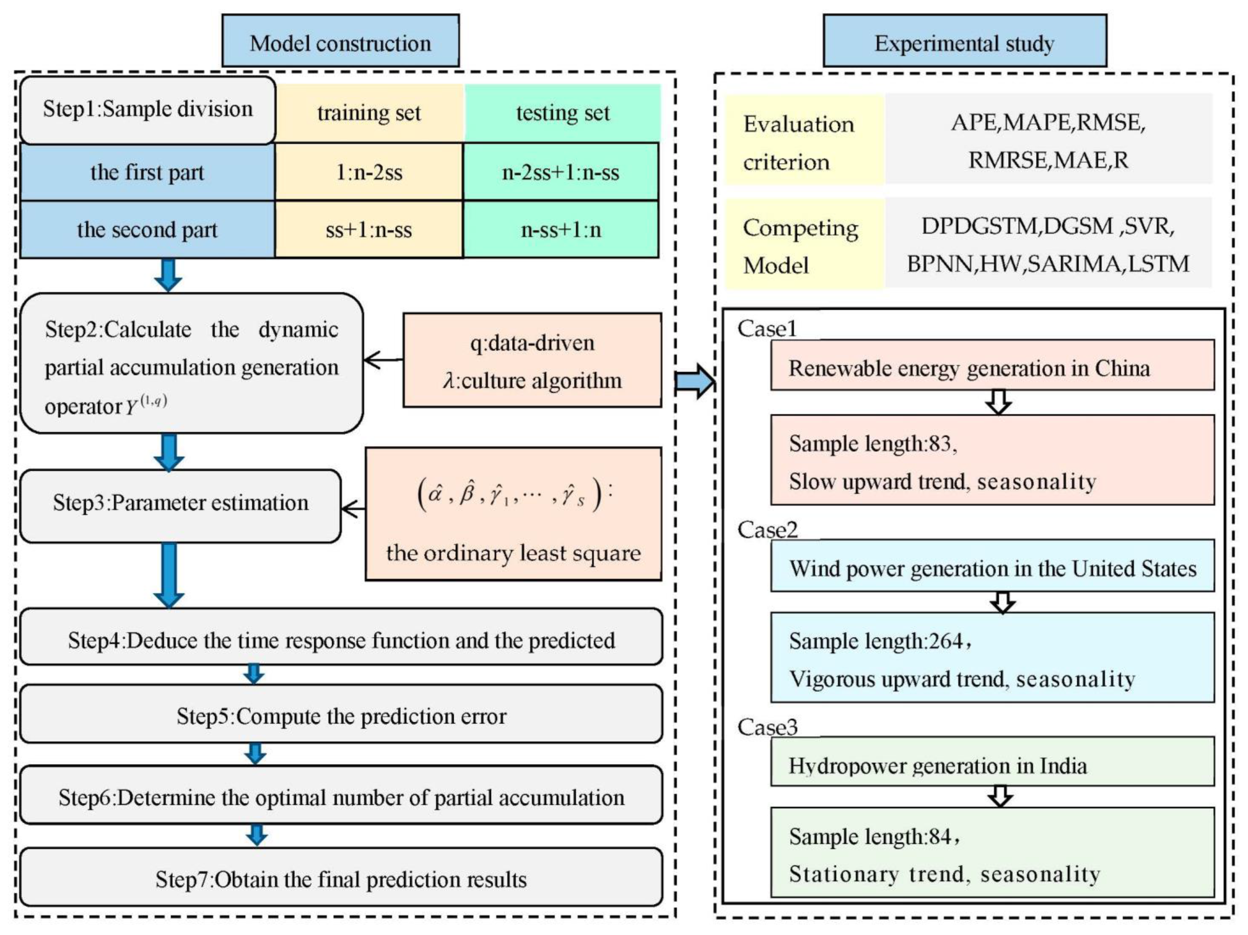
The modeling process of the DPSGSTM(1,1) can be summarized as the following steps.

Step 1: Sample division. Assume that $X^{(0)}=\left(x^{\left(0\right)}\left(1\right),x^{\left(0\right)}\left(2\right),\cdots ,x^{\left(0\right)}\left(n-ss\right)\right)$ is raw data. As shown in Figure 1, split $X^{(0)}$ into two sections, i.e., $x^{\left(0\right)}\left(1:\left(n-ss\right)\right)$ is the first part and $x^{\left(0\right)}\left(\left(ss+1\right):n\right)$ is the second part. Subsequently, based on the first division, each section is again divided into a training set and a testing set, i.e.,$x^{\left(0\right)}\left(\left(ss+1\right):\left(n-2ss\right)\right)$ and $x^{\left(0\right)}\left(\left(n-2ss+1\right):\left(n-ss\right)\right)$, respectively, represent the training set and testing set for the first part data, and $x^{\left(0\right)}\left(\left(ss+1\right):\left(n-ss\right)\right)$ and $x^{\left(0\right)}\left(\left(n-ss+1\right):n\right)$, respectively, represent the training set and testing set for the second part data.

Step 2: Dynamic partial accumulation generation. Set the accumulation starting point $qq$ from range $q=3,4,\cdots ,n-2ss-s-2$, for example $qq=3$. Subsequently, according to the optimization equation of Equation (9), the culture algorithm is used to find the hyperparameter $\lambda$. Finally, calculate one order dynamic partial accumulation generation sequence $Y^{(1,3)}=y^{(1,3)}\left(1\right),y^{(1,3)}\left(2\right),\cdots ,y^{(1,3)}\left(n-2ss-2\right)$ of $x^{\left(0\right)}\left(1:\left(n-2ss\right)\right)$ according to Equation (1).

Step 3: Parameter solution. Substitute $Y^{(1,3)}$ into Equation (5) and employ the ordinary least square method to solve the parameter vector $A=\left(\widehat{\alpha },\widehat{\beta },{\widehat{\gamma }}_1,{\widehat{\gamma }}_2\cdots ,{\widehat{\gamma }}_S\right)$.

Step 4: Calculate the time response equation and predicted value. Bring the parameter vector $A=\left(\widehat{\alpha },\widehat{\beta },{\widehat{\gamma }}_1,{\widehat{\gamma }}_2\cdots ,{\widehat{\gamma }}_S\right)$ solved by Step 4 into Equation (6), and then calculate the time response equation, i.e., ${\widehat{Y}}^{(1,3)}={\widehat{y}}^{(1,3)}\left(1\right),{\widehat{y}}^{(1,3)}\left(2\right),\cdots ,{\widehat{y}}^{(1,3)}\left(n-ss-2\right)$. Then, obtain the predicted value by the reverse dynamic partial accumulation generation operator in Equation (2), i.e., $\widehat{X}={\widehat{x}}^{(0)}\left(1\right),{\widehat{x}}^{(0)}\left(2\right),\cdots ,{\widehat{x}}^{(0)}\left(n-ss\right)$.

Step 5: Evaluate prediction error. Compute the MAPE value between the predicted value, i.e.,${\widehat{x}}^{\left(0\right)}\left(n-2ss+1\right),{\widehat{x}}^{\left(0\right)}\left(n-2ss+2\right),\cdots ,{\widehat{x}}^{\left(0\right)}\left(n-ss\right)$ and the testing set, i.e., $x^{\left(0\right)}\left(n-2ss+1\right),x^{\left(0\right)}\left(n-2ss+2\right),\cdots ,x^{\left(0\right)}\left(n-ss\right)$ for the first part data.

Step 6: Determine the optimal number of partial accumulations. For the training set for the first part data, i.e., $x^{\left(0\right)}\left(1:\left(n-ss\right)\right)$, select the next q value, i.e., $q=4$ from accumulation domain and repeat step 2–6. Based on minimizing MAPE, determine the optimal q value(zyq) and corresponding $\lambda$.

Step 7: Obtain the final prediction results. For the second part data, i.e., $x^{\left(0\right)}\left(\left(ss+1\right):n\right)$, substitute zyq and corresponding $\lambda$ into Equation (1), and the dynamic partial accumulation generation sequence $Y^{(1,zyq)}$ can be obtained. Subsequently, according to the step 3, the parameter vector $A=\left(\widehat{\alpha },\widehat{\beta },{\widehat{\gamma }}_1,{\widehat{\gamma }}_2\cdots ,{\widehat{\gamma }}_S\right)$ can be solved. Finally, repeat step 5–6 and then the final prediction results can be calculated.

4. Experimental Study

4.1. Experimental Design

With the increasing share of electricity in global end-energy consumption, developing renewable energy power generation is an important way to achieve the transformation of energy structure and high-quality economic development. The power generation structure of renewable energy includes hydropower, wind power, solar power, and biomass power generation, etc. Due to the fluctuation of output power and the limitation of climate conditions, the renewable energy generation sequence presents complex features such as nonlinear trend and periodic fluctuation. It is imperative to develop a reliable and stable renewable energy generation forecasting technology to facilitate the safe supply and flexible scheduling of electricity system. Consequently, in order to reasonably predict the development trend of renewable energy generation, this paper builds a novel grey seasonal model, namely DPDGSTM(1,1).

For verification purposes, the new-established model is applied to power prediction for three countries with strong generation capacity: renewable energy generation in China, wind power generation in the United States, and hydropower generation in India. Case 1 selects the total amount of renewable energy power generation in China, including tidal, wind and solar energy. Case two uses net wind power generation data from independent power plants in the United States. The third case is Indian hydropower generation. The three cases are accompanied by different sample lengths, development trends, and seasonal fluctuations, which can comprehensively validate the prediction ability of the new model under different scenarios. The data sources for three cases are the international energy agency, the energy information administration, and the Central Power Authority of India, respectively.

Furthermore, five benchmark models are compared with the new model, namely the grey model DGSM(1,1), time series model Holt-Winters and SARIMA, statistical learning model SVR, and machine learning model BPNN. The reason for choosing these prevailing benchmarks is that the grey model DGSM can effectively identify the seasonal fluctuation in small samples, while the BPNN and SVR are representative models for dealing with nonlinear sequences. In addition, Holt-Winters and SARIMA are widely used time series models.

Finally,

Table 1. Data division.

a
Benchmark Model	Country	Sample Length	Training Set	Testing Set	Forecasting Horizon
	China	83	1 January 2016–31 December 2021	1 January 2022–31 November 2022	11
	The United states	264	1 January 2001–31 December 2021	1 January 2022–31 December 2022	12
	India	84	1 January 2016–31 December 2021	1 January 2022–31 December 2022	12
b
New Model	Country	Division	Training Set	Testing Set	Forecasting Horizon
	China	First part	1 January 2016–31 December 2020	1 January 2021–31 December 2021	12
		Second part	1 January 2017–31 December 2021	1 January 2022–31 November 2022	11
	The United states	First part	1 January 2001–31 December 2020	1 January 2021–31 December 2021	12
		Second part	1 January 2002–31 December 2021	1 January 2022–31 December 2022	12
	India	First part	1 January 2016–31 December 2020	1 January 2021–31 December 2021	12
		Second part	1 January 2017–31 December 2021	1 January 2022–31 December 2022	12

shows the detailed information for three cases, including sample length, data division, and prediction horizon. Each sample is divided into a training set and a testing set for simulating and validating original data. Due to the availability of data, China’s renewable energy power generation data is only updated until November 2022, so the prediction horizon of China’s case is 11, while that of the US and India is predicted one cycle later, namely 12 months.

4.2. Parameter Estimation and Evaluation Criterion

In this paper, the monthly data of renewable energy generation in China is taken as an example to illustrate the parameter estimation of competing models, as shown in

Table 2. Parameter estimation of renewable energy generation in China.

Models	Parameter
DPDGSTM(1,1)	$\widehat{\mathsf{\alpha }}=0.3289, \widehat{\mathsf{\beta }}=\mathrm{29,974.6504}, {\widehat{\mathsf{\gamma }}}_1=\mathrm{3,646,901.8149}, {\widehat{\mathsf{\gamma }}}_2=\mathrm{3,628,612.9366}, {\widehat{\mathsf{\gamma }}}_3=\mathrm{3,633,499.2547},$ ${\widehat{\mathsf{\gamma }}}_4=\mathrm{3,628,447.64203}, {\widehat{\mathsf{\gamma }}}_5=\mathrm{3,628,179.9937}, {\widehat{\mathsf{\gamma }}}_6=\mathrm{3,634,321.8452},$ ${{\widehat{\mathsf{\gamma }}}_7=\mathrm{3,641,360.8393}, \widehat{\mathsf{\gamma }}}_8=\mathrm{3,646,589.5148}, {\widehat{\mathsf{\gamma }}}_9=\mathrm{3,657,317.1157},$ ${\widehat{\mathsf{\gamma }}}_{10}=\mathrm{3,663,069.8349}, {\widehat{\mathsf{\gamma }}}_{11}=\mathrm{3,655,327.7906}, {\widehat{\mathsf{\gamma }}}_{12}=\mathrm{3,653,502.8356},$ the optimal q = 36,$\mathsf{\lambda }=1$.
DGSM(1,1)	$\widehat{\mathsf{\alpha }}=1.0077, {\widehat{\mathsf{\beta }}}_1=\mathrm{92,987.6943}, {\widehat{\mathsf{\beta }}}_2=\mathrm{81,216.9853}, {\widehat{\mathsf{\beta }}}_3=\mathrm{105,943.1222}, {\widehat{\mathsf{\beta }}}_4=\mathrm{108,299.1560},$ ${\widehat{\mathsf{\beta }}}_5=\mathrm{127,084.6777}, {\widehat{\mathsf{\beta }}}_6=\mathrm{137,207.9494}, {\widehat{\mathsf{\beta }}}_7=\mathrm{159,057.9306}, {\widehat{\mathsf{\beta }}}_8=\mathrm{148,310.6635},$ ${\widehat{\mathsf{\beta }}}_9=\mathrm{137,508.4139}, {\widehat{\mathsf{\beta }}}_{10}=\mathrm{134,807.5482}, {\widehat{\mathsf{\beta }}}_{11}=\mathrm{109,272.6660}, {\widehat{\mathsf{\beta }}}_{12}=\mathrm{95,680.7670}.$
SVR	The embedding dimension $\mathrm{w} \in$[1, 24], the time lag $\mathsf{\tau } \in$[1, 8], the optimal $\mathrm{w}$ = 13, the optimal $\mathsf{\tau }$ = 1, RBF kernel, $\mathrm{c} \in$[0.1, 1000], $\mathsf{\gamma } \in$[0.1, 500], the optimal $\widehat{\mathrm{c}}=5.6569$, the optimal $\widehat{\mathsf{\gamma }}=0.0625$.
BPNN	The embedding dimension $\mathrm{w} \in$[1, 24], the time lag $\mathsf{\tau } \in$[1, 8], the optimal $\mathrm{w}$ = 9, the optimal $\mathsf{\tau }$ = 1, the number of neuros $\mathrm{g} \in$[4, 252], the optimal $\mathrm{g}$ = 14, learning rate = 0.001, the epochs iteration = 1000, error goal = 0.05.
Holt-Winters	$\mathsf{\alpha } \in$[0, 1], $\mathsf{\beta } \in$[0, 1],$\mathsf{\delta } \in$[0, 1], the optimization algorithm = “L-BFGS-B”, $\mathrm{t}\mathrm{h}\mathrm{e} \mathrm{o}\mathrm{p}\mathrm{t}\mathrm{i}\mathrm{m}\mathrm{a}\mathrm{l} \widehat{\mathsf{\alpha }}=0.5307,$ $\mathrm{t}\mathrm{h}\mathrm{e} \mathrm{o}\mathrm{p}\mathrm{t}\mathrm{i}\mathrm{m}\mathrm{a}\mathrm{l} \widehat{\mathsf{\beta }}=0$, $\mathrm{t}\mathrm{h}\mathrm{e} \mathrm{o}\mathrm{p}\mathrm{t}\mathrm{i}\mathrm{m}\mathrm{a}\mathrm{l} \widehat{\mathsf{\delta }}=0.7485$.
SARIMA	${\mathrm{S}\mathrm{A}\mathrm{R}\mathrm{I}\mathrm{M}\mathrm{A}(3,0,0)(3,0,0)}_{12}$, AR(3) = 0.3466 **, AIC = −2.5211, Log L = 78.6343.
LSTM	Embedding dimension $\mathrm{m} ϵ [2,12]$, time lag $\mathsf{\tau } ϵ [1,2]$, optimal m = 8, optimal $\mathsf{\tau }$ = 1, optimizers = Adam, learning rate = 0.001, decay = $1\times {10}^{-6}$ two hidden layers, the number of neurons in the first and second layer = 8 and 4, loss = ‘mean_squared_error’, epochs = 100, batch_size = 1.

Note: the ** denotes the p-value of the corresponding parameter is less than 5%.

. For the other two cases, their parameter estimation process is analogous to the Chinese case, and the corresponding parameter estimation results are presented in Appendix A. Initially, the parameters of the new model include two hyperparameters and a parameter vector. The two hyperparameters are, respectively, the partial accumulation number $q$ and the accumulation order $\lambda$ that can measure the weight of the new and old information in a period. The partial accumulation number $q$ can be calculated based on the data-driven idea and the accumulation order $\lambda$ can be searched by the cultural algorithm. For the parameter vector $A=\left(\alpha ,\beta ,{\gamma }_1,{\gamma }_2,\cdots ,{\gamma }_{12}\right)$, where $\alpha$ represents development coefficient and $\beta t$ represents the time trend term that can reflect the effects of time trends on the system series. In addition, ${\gamma }_{M_{\left(t+q,s\right)}}$ represents dummy variables to capture the seasonal fluctuations of the time series. For instance, s = 12 represents the monthly sequence and the corresponding parameter vector is $A=\left(\alpha ,\beta ,{\gamma }_1,{\gamma }_2,\cdots ,{\gamma }_{12}\right)$. For the grey model DGSM(1,1), the least square method is used to solve the parameters, where $\alpha$ represents the development coefficient which can reflect the development trend of the system and $\beta$ denotes the seasonal parameter. For the SVR model, after comparing the prediction performance of the linear kernel, polynomial kernel, and RBF kernel functions, the RBF kernel is finally utilized in the SVR model. Moreover, the optimal combination of the penalty parameter $c$ and the width parameter $\gamma$ are searched by the cross-validation method. Given that the SVR and BPNN are multi-variable input models, and the modeling sequence is a univariable time series, this research performed phase space transformation on the time series by introducing embedding dimension and time lag term, and then uses the grid search method to find the optimal hyperparameters. Moreover, the SARIMA model first finds the optimal order based on the autocorrelation function, partial autocorrelation function, and AIC criterion. The parameter in SARIMA model is estimated using the maximum likelihood function. A heteroskedasticity test on the modeling error is further used to judge the rationality of the model. The Holt-Winters package in R is applied to build the Holt-Winters(HW) model.

Furthermore, six evaluation criteria are employed to evaluate the prediction performance of the competing models, which are absolute percent error (APE), mean absolute percent error for simulation (MAPES) and prediction (MAPEP), root mean squared error for simulation (RMSES) and prediction (RMSEP), root mean relative squared error for simulation (RMRSES) and prediction (RMRSEP), mean absolute error for simulation(MAES) and prediction(MAEP), and Pearson coefficient for simulation(RS) and prediction(RP), respectively. The corresponding formulas are displayed as follows:

$$\begin{array}{l}APE(t)=\left|\frac{{\widehat{x}}^{\left(0\right)}\left(t\right)-x^{\left(0\right)}\left(t\right)}{x^{\left(0\right)}\left(t\right)}\right|\times 100\%,t=1,2,\cdots ,n+ss\\ MAPES=\frac{1}{n}{\displaystyle \sum _{t=1}^{n}APE\left(t\right)}, MAPEP=\frac{1}{ss}{\displaystyle \sum _{t=1}^{ss}APE\left(t\right)}\\ RMSES=\sqrt{\frac{1}{n}{{\displaystyle \sum _{t=1}^n\left({\widehat{x}}^{\left(0\right)}\left(t\right)-x^{\left(0\right)}\left(t\right)\right)}}^2}, RMSEP=\sqrt{\frac{1}{ss}{{\displaystyle \sum _{t=1}^{ss}\left({\widehat{x}}^{\left(0\right)}\left(t\right)-x^{\left(0\right)}\left(t\right)\right)}}^2}\\ RMRSES=\sqrt{\frac{1}{n}{\displaystyle \sum _{t=1}^{n}AP{E}^2}}, RMRSEP=\sqrt{\frac{1}{SS}{\displaystyle \sum _{t=1}^{SS}AP{E}^2}}\\ MAES=\frac{1}{n}{\displaystyle \sum _{t=1}^n\left|{\widehat{x}}^{\left(0\right)}\left(t\right)-x^{\left(0\right)}\left(t\right)\right|}, MAEP=\frac{1}{ss}{\displaystyle \sum _{t=1}^{ss}\left|{\widehat{x}}^{\left(0\right)}\left(t\right)-x^{\left(0\right)}\left(t\right)\right|}\\ RS=\frac{{\displaystyle \sum _{i=1}^n\left(x^{\left(0\right)}\left(t\right)-{\overline{x}}^{\left(0\right)}\left(t\right)\right)\left(x\left(t\right)-\overline{x}\left(t\right)\right)}}{\sqrt{{\displaystyle \sum _{t=1}^n{\left(x^{\left(0\right)}\left(t\right)-{\overline{x}}^{\left(0\right)}\left(t\right)\right)}^2}}\sqrt{{\displaystyle \sum _{t=1}^n{\left(y^{\left(0\right)}\left(t\right)-{\overline{y}}^{\left(0\right)}\left(t\right)\right)}^2}}},\\ RP=\frac{{\displaystyle \sum _{i=1}^{ss}\left(x^{\left(0\right)}\left(t\right)-{\overline{x}}^{\left(0\right)}\left(t\right)\right)\left(x\left(t\right)-\overline{x}\left(t\right)\right)}}{\sqrt{{\displaystyle \sum _{t=1}^{ss}{\left(x^{\left(0\right)}\left(t\right)-{\overline{x}}^{\left(0\right)}\left(t\right)\right)}^2}}\sqrt{{\displaystyle \sum _{t=1}^{ss}{\left(y^{\left(0\right)}\left(t\right)-{\overline{y}}^{\left(0\right)}\left(t\right)\right)}^2}}}\end{array}$$

(10)

where n represents the size of training set and ss denotes the length of prediction horizon. The smaller the MAPE, RMSE, RMRSE, MAE value, the higher the prediction accuracy of a certain model. APE is used to measure the robustness of the model prediction results. The smaller the maximum APE is, the smaller the deviation degree of the prediction value from the original value and the higher the prediction stability of a certain model. The greater the R value, the higher the degree of correlation between the predicted value and the original value.

4.3. Case Analysis

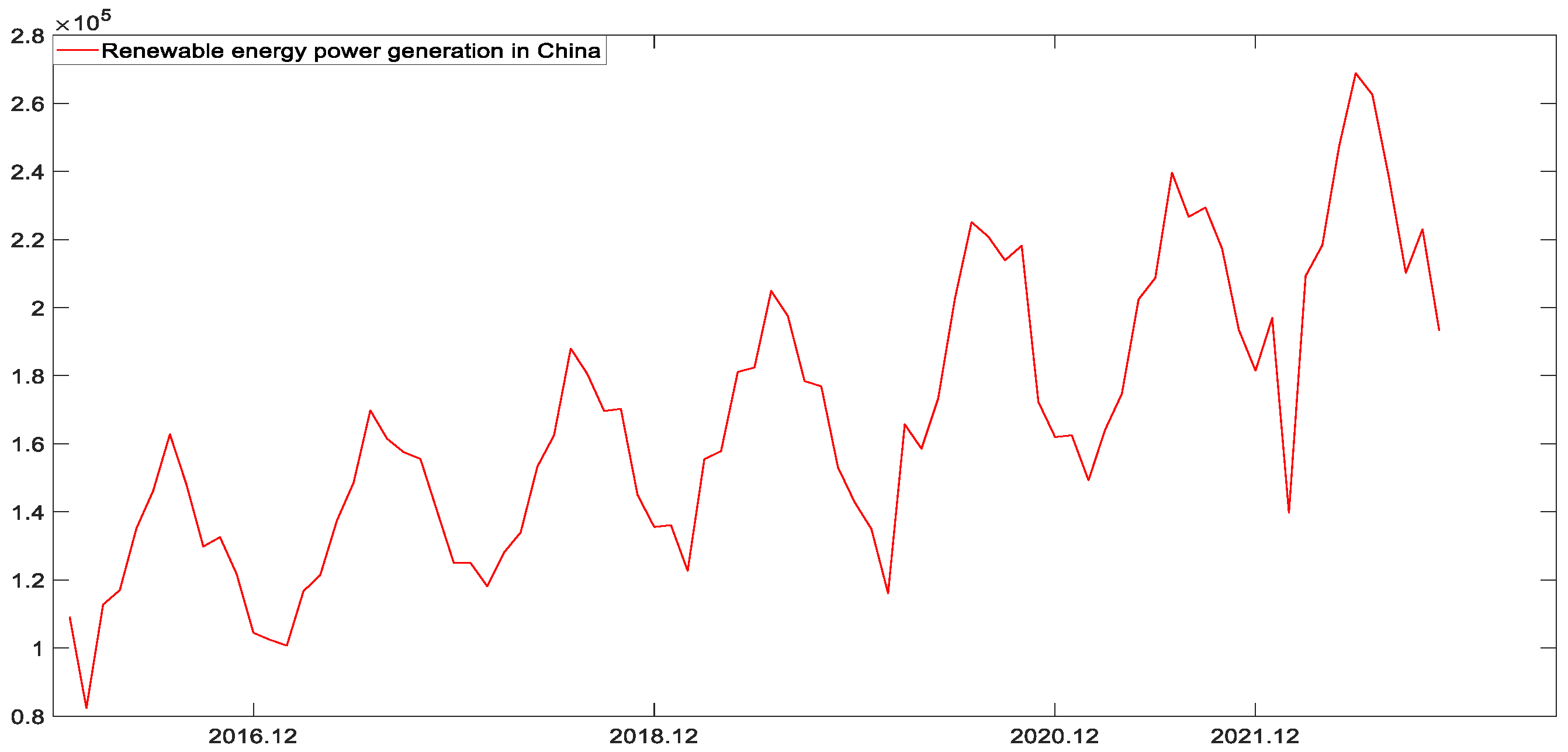
4.3.1. Case 1: Monthly Prediction of Renewable Energy Generation in China

Figure 2 presents China’s renewable energy generation, it can be seen that the sequence exhibits strong seasonality and slow upward trend.

Step 1 Data division. There are 83 data points in China’s renewable energy generation series, with a time span of 1 January 2016–31 November 2022. Firstly, the data of China’s renewable energy generation is divided into two parts. Data points 1–72 (i.e., 1 January 2016–31 December 2021) are taken as the first part of the data to determine the hyperparameters of the model, including the optimal accumulation number and $\lambda$. Data points 13–83 (i.e., 1 January 2017–31 November 2022) are taken as the second part of data for training and testing the modeling effect. Secondly, the two partial data are divided into the training set and the test set again. The specific data division is shown in Table 1

Step 2 Dynamic partial accumulation generation. First of all, the accumulation start point is set as 31 in this case. Subsequently, according to the constraint conditions of Equation (9), the optimal hyperparameter $\lambda =0.3244$ can be sought by using culture algorithm. Finally, according to Equation (1), the dynamic partial accumulation generation sequence for the training set of the first part data can be calculated, i.e., $Y^{(1,31)}=y^{(1,31)}\left(1\right),y^{(1,31)}\left(2\right),\cdots ,y^{(1,31)}\left(30\right)$.

Step 3 Parameter solution. The parameter matrix is constructed according to Equation (5), and the parameter vector can be estimated by the least square method.

$$\begin{array}{l}B=\left[\begin{array}{cccccc}{y}^{(1,q)}(1)& 1& I_{M(32,12)=1}& I_{M(32,12)=2}& \cdots & I_{M(32,12)=12}\\ y^{(1,q)}(2)& 2& I_{M(33,12)=1}& I_{M(33,12)=2}& \cdots & I_{M(33,12)=12}\\ ⋮& ⋮& ⋮& ⋮& ⋮& ⋮\\ y^{(1,q)}(29)& 29& I_{M(60,12)=1}& I_{M(60,12)=2}& \cdots & I_{M(60,12)=12}\end{array}\right]Y=\left[\begin{array}{c}{y}^{\left(1,q\right)}\left(2\right)\\ y^{\left(1,q\right)}\left(3\right)\\ ⋮\\ y^{\left(1,q\right)}\left(30\right)\end{array}\right]\\ \begin{array}{l}A=\left(\widehat{\alpha },\widehat{\beta },{\widehat{\gamma }}_1,{\widehat{\gamma }}_2\cdots ,{\widehat{\gamma }}_{12}\right)\\ =[0.81,374.13,27305.00,15394.98,65532.29,45880.21,60206.10,\\ 64530.18,75827.00,54447.75,40159.55,46319.47,15497.97,22453.89]\end{array}\end{array}$$

Step 4 Substitute $Y^{(1,31)}$ into Equation (6) to calculate the corresponding time equation as follows.

$${\widehat{y}}^{\left(1,31\right)}\left(t+1\right)={0.81}^t{y}^{\left(1,31\right)}\left(1\right)+{\displaystyle \sum _{m=1}^t{0.81}^{t-m}\left[374.13m+{\widehat{\gamma }}_{M\left(m+31,12\right)}\right]}$$

Then, according to Equation (2), the simulated and predicted value ${\widehat{X}}^{\left(0\right)}$ can be obtained by calculating the reverse dynamic partial accumulation generation for $Y^{(1,31)}$.

Step 5 According the equation, the following will obtain the prediction error of the new model.

$$MAPEP=\frac{1}{n}{\displaystyle \sum _{t=1}^n\left|\frac{{\widehat{x}}^{\left(0\right)}\left(t\right)-x^{\left(0\right)}\left(t\right)}{x^{\left(0\right)}\left(t\right)}\right|\ast 100\%}=\frac{1}{12}{\displaystyle \sum _{t=61}^{72}\left|\frac{{\widehat{x}}^{\left(0\right)}\left(t\right)-x^{\left(0\right)}\left(t\right)}{x^{\left(0\right)}\left(t\right)}\right|}\ast 100\%$$

Step 6 For the first part of the data, go through the accumulation range and repeat steps 2–5, and then the optimal $q=36$ and $\lambda =1$ can be obtained based on the principle of minimum MAPE.

Step 7 For the second part of the data, the optimal partial accumulations number and the corresponding $\lambda$ are bought into Equation (1) to calculate the accumulation sequence for the training set of the second part data, and then repeat steps 2–5 for the second part data to obtain the final prediction results.

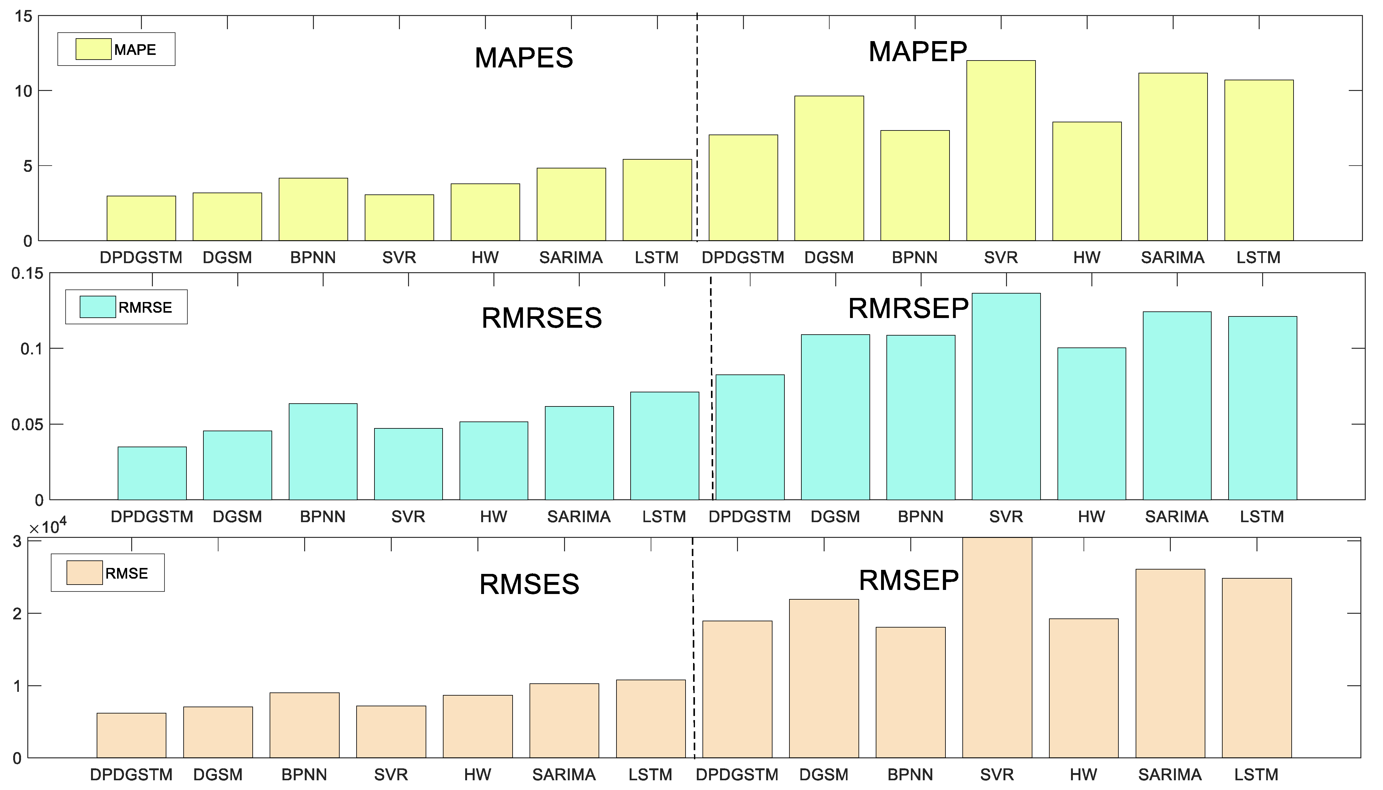
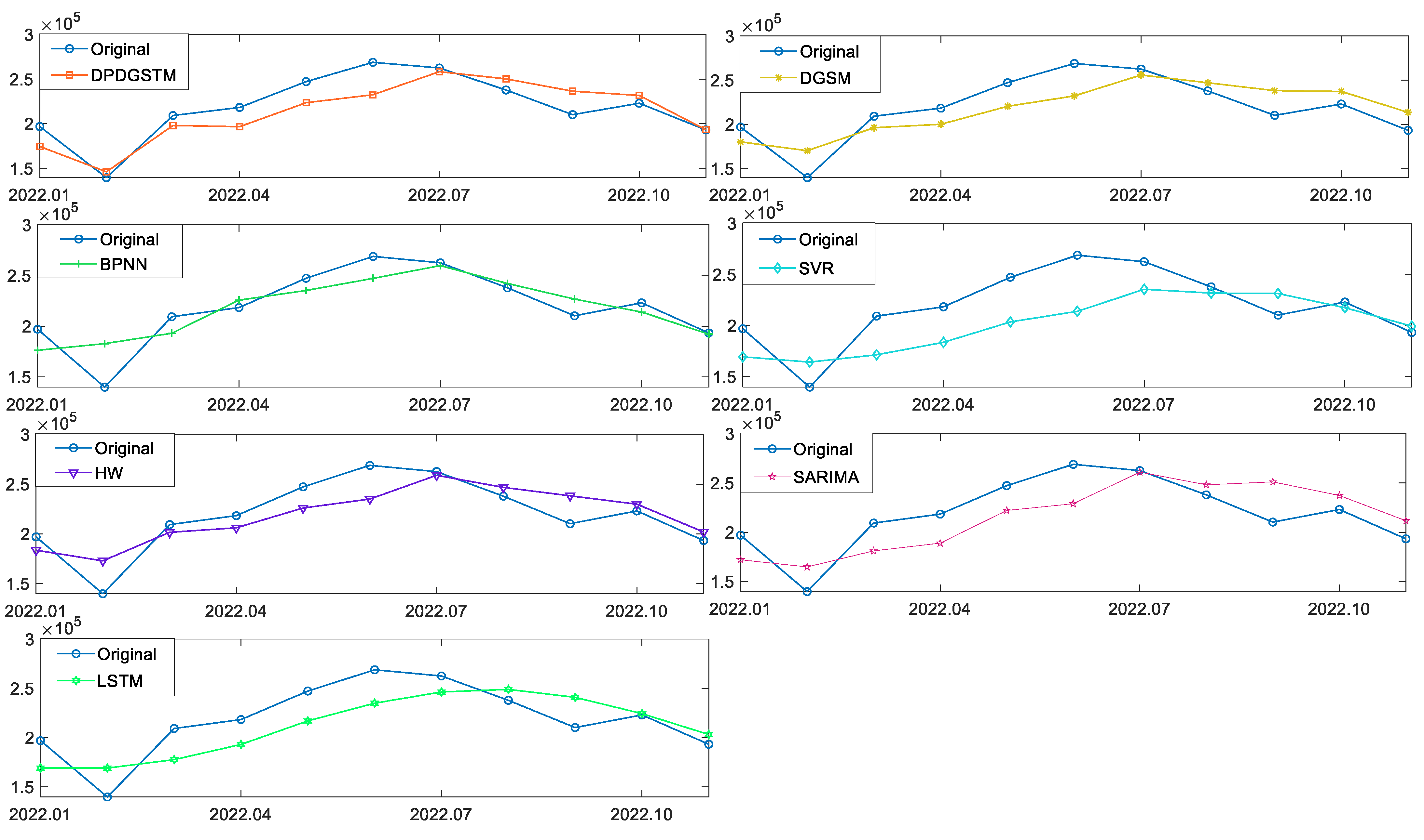
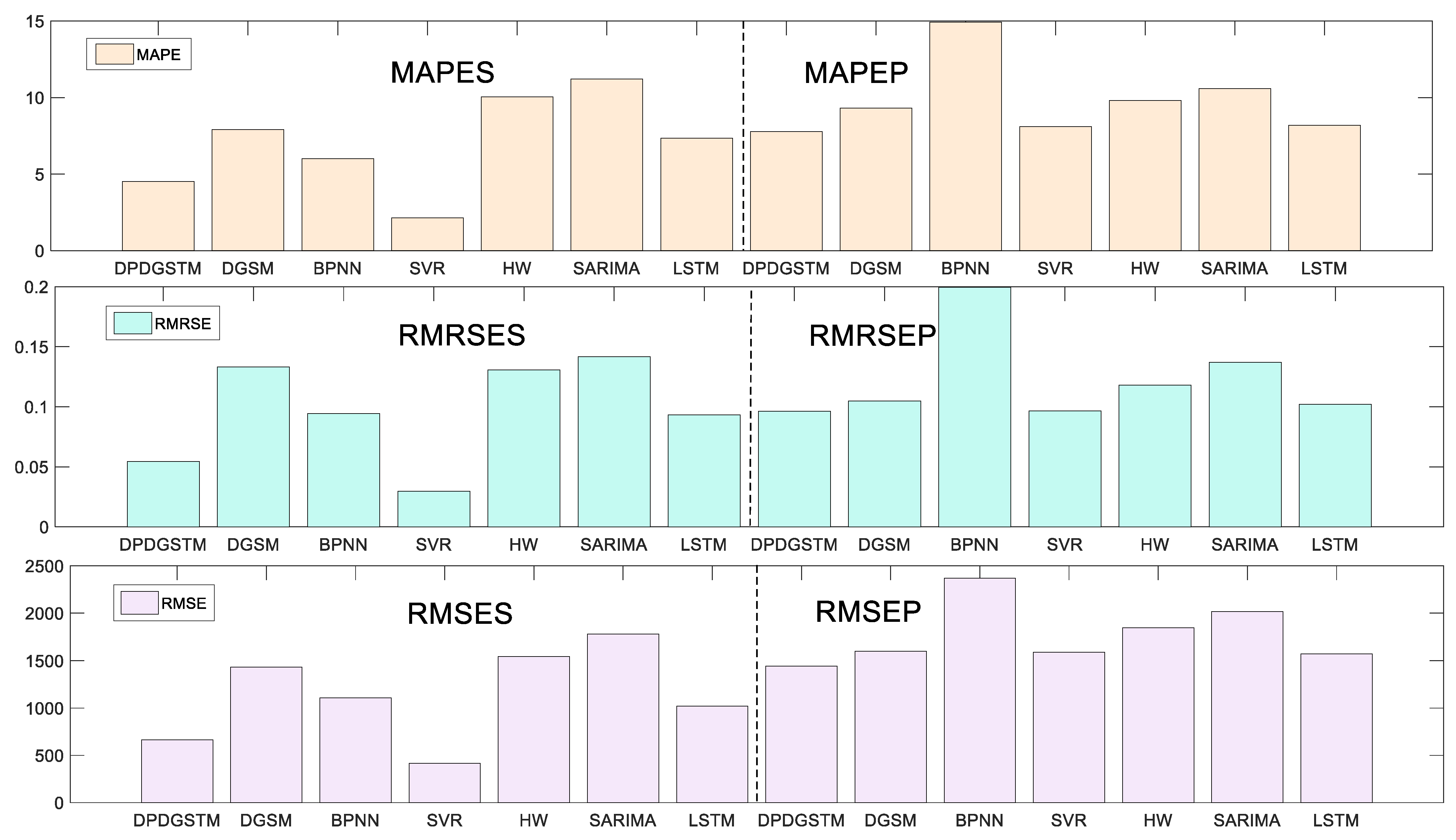
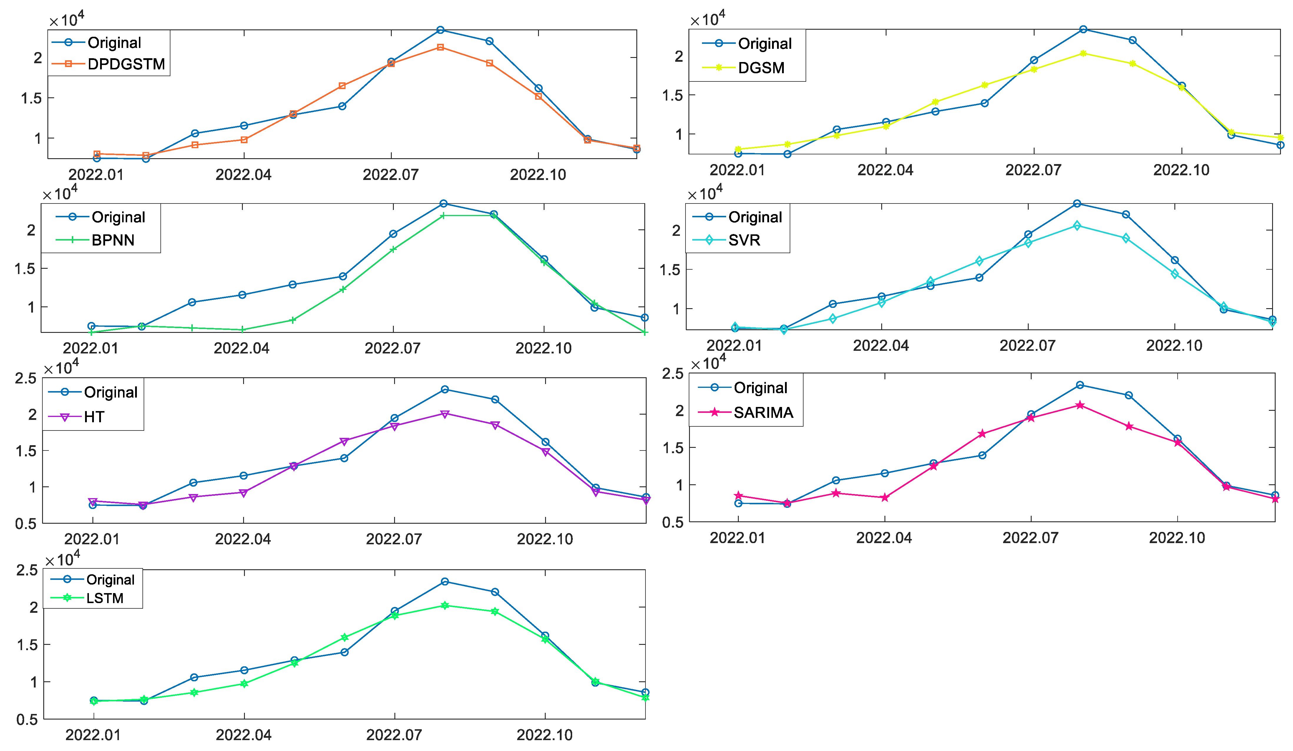
According to the prediction performance of each model, the error comparison in Figure 3 and the prediction curve graph in Figure 4 are drawn. The detailed prediction results of each model are shown in

Table 3. Prediction results of competing models in China.

Month	Original	DPDGSTM	APE	DGSM	APE	BPNN	APE	SVR	APE	HW	APE	SARIMA	APE	LSTM	APE
31 January 2022	196,927.39	174,631.11	11.32	180,155.11	8.52	176,129.80	10.56	169,428.00	13.96	183,547.80	6.79	172,001.72	12.66	169,120.97	14.12
28 February 2022	139,733.63	146,226.55	4.65	170,202.17	21.8	182,702.50	30.75	164,266.07	17.56	172,862.10	23.71	164,731.41	17.89	169,082.09	21
31 March 2022	209,262.64	198,102.56	5.33	196,230.41	6.23	192,992.84	7.77	171,414.50	18.09	201,496.80	3.71	181,002.39	13.5	177,650.41	15.11
30 April 2022	218,318.50	196,804.54	9.85	200,087.68	8.35	225,657.91	3.36	183,593.39	15.91	206,076.40	5.61	188,868.62	13.49	193,066.53	11.57
31 May 2022	247,232.68	223,625.40	9.55	220,403.94	10.85	235,192.01	4.87	203,573.89	17.66	225,975.50	8.6	222,034.63	10.19	216,969.69	12.24
30 June 2022	268,854.14	232,506.22	13.52	232,213.38	13.63	247,162.44	8.07	213,935.34	20.43	234,972.30	12.6	228,855.11	14.88	234,964.27	12.61
31 July 2022	262,518.97	258,342.81	1.59	255,839.88	2.54	259,716.02	1.07	235,490.38	10.3	258,870.70	1.39	260,952.59	0.6	246,333.42	6.17
31 August 2022	237,867.88	250,281.41	5.22	247,049.87	3.86	242,125.87	1.79	231,800.36	2.55	246,701.20	3.71	248,097.87	4.3	248,949.76	4.66
30 September 2022	210,207.38	236,498.90	12.51	238,137.64	13.29	226,694.54	7.84	231,366.82	10.07	238,231.30	13.33	251,046.76	19.43	240,877.27	14.59
31 October 2022	223,013.25	231,723.43	3.91	237,258.61	6.39	213,876.37	4.1	217,495.50	2.47	229,805.90	3.05	237,253.18	6.39	224,352.50	0.6
30 November 2022	193,234.12	193,406.35	0.09	213,538.84	10.51	192,099.21	0.59	199,391.89	3.19	201,852.30	4.46	211,613.20	9.51	203,121.10	5.12
MAPES		2.9773		3.1738		4.1574		3.0567		3.7801		4.8301		5.4177
RMRSES		0.0349		0.0454		0.0636		0.0472		0.0514		0.0616		0.0711
RMSES		6205.199		7058.9118		9004.0399		7161.4433		8646.0974		10,281.45		10,765.89
MAES		5393.6864		4933.958		6419.8707		4941.4576		6333.75		8050.8202		8391.5545
RS		0.9815		0.9802		0.9672		0.9764		0.9681		0.9499		0.9547
MAPEP		7.0487		9.6334		7.3429		12.0157		7.9056		11.1666		10.7067
RMRSEP		0.0826		0.1091		0.1087		0.1363		0.1004		0.1242		0.121
RMSEP		18,934.89		18,928.59		18,929.59		18,930.59		18,931.59		18,932.59		18,933.59
MAEP		15,743.83		20,028.62		14,084.36		26,283.07		16,142.85		23,462.31		22,485.05
RP		0.8581		0.774		0.857		0.6815		0.8356		0.7047		0.738

. Table 3 is divided into two parts, the upper part of the table presents the prediction values of the new model and competing models, as well as the absolute percentage error (APE), corresponding to each point of the prediction phase. The lower part shows the forecasting ability of the competing models in the fitting and prediction stages under different evaluation criteria. For the MAPE, RMSE, RMRSE and MAE indicators, their smaller values represent a lower prediction error and better prediction performance. For the Pearson coefficient, the larger its value, the higher the correlation degree between the prediction results and the original values.

As can be seen from Figure 3, in the fitting stage, the seven models have high fitting accuracy with all MAPES less than 6%. Among them, the new model (DPDGSTM(1,1)) has the smallest MAPES, RMSES, RMRSES and the highest Pearson coefficient. As can be seen from Figure 4 and Table 3, in the prediction stage, the new model has the smallest MAPEP and RMESEP and the highest Pearson coefficient, suggesting robust and superior prediction ability. For BPNN and Holt-Winters models, their prediction accuracies are ranked second and third. Especially, BPNN has the smallest RMSEP and MAEP, and can be used as the suboptimal alternative model to predict China’s renewable energy generation. However, the APE error range of BPNN is larger than that of the new model which shows that the predictive stability of BPNN is not as good as that of the new model. In addition, the error indicators of the grey seasonal model DGSM(1,1) in the prediction phases are significantly higher than those of the new model, indicating that the introduction of dynamic partial accumulation operator and time trend term can effectively improve the prediction ability of the grey model for nonlinear fluctuation series. Finally, for the SARIMA, LSTM, and SVR models, prediction performance is poor in this case. Although the SVR and BPNN have ideal fitting accuracy, it seems to fall into the overfitting problem. For the SARIMA model, fixed linear structure limits its prediction accuracy in energy generation series with a nonlinear growth trend.

4.3.2. Case 2: Monthly Prediction of Wind Power Generation in the United States

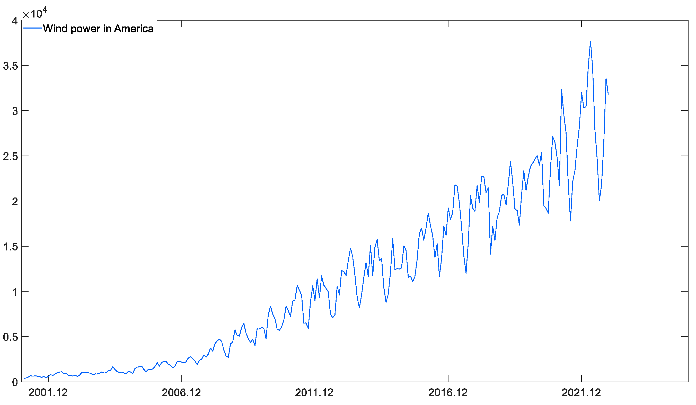
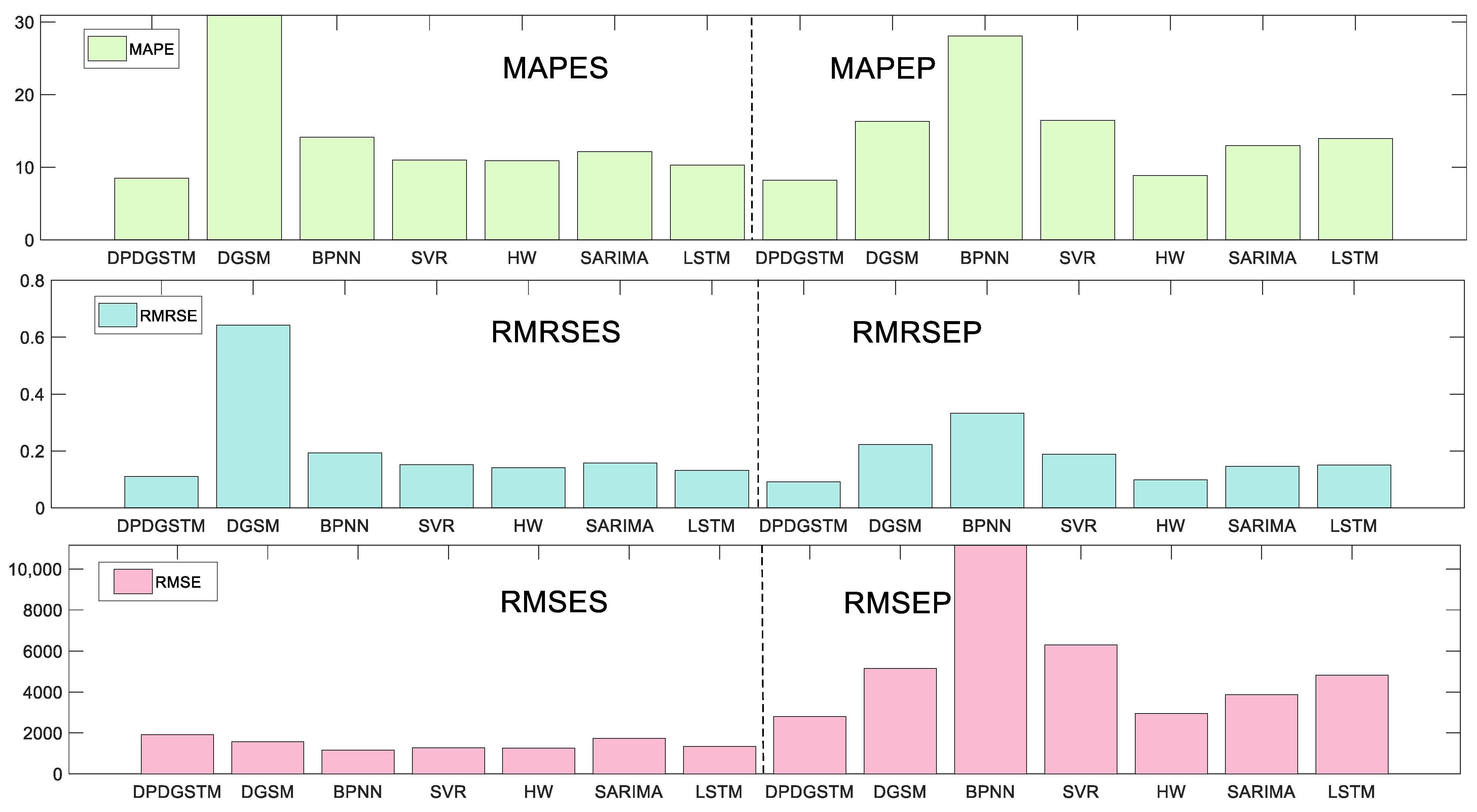
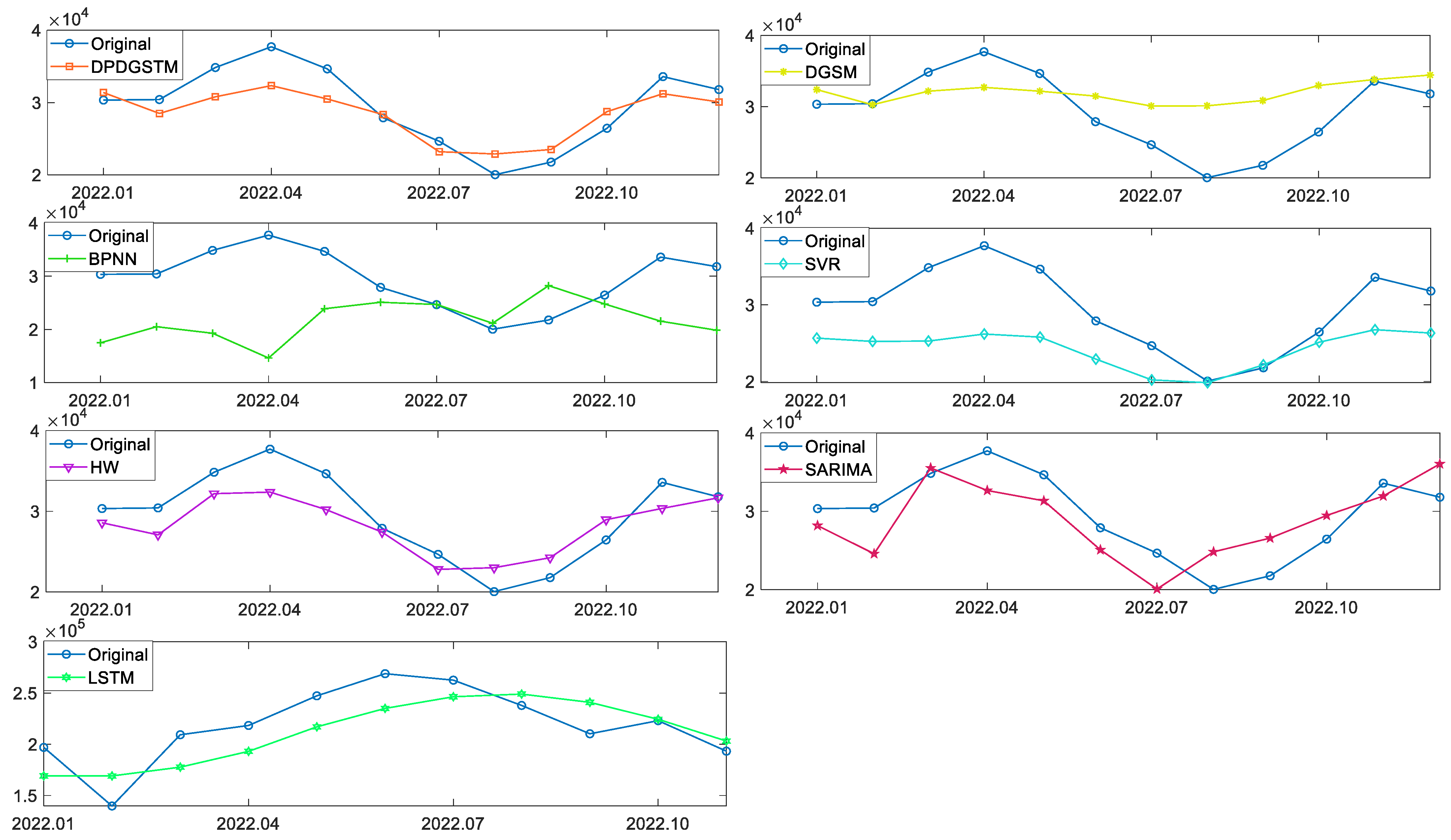
As Figure 5 shows, the wind power generation in the United States increases with a quasi-exponential growth trend during 2001–2022. In 2021, the United States had the second highest newly wind power installed capacity in world, and its wind power has become an important source of power generation.

Table 4. Prediction results of competing models in the United States.

Month	Original	DPDGSTM	APE	DGSM	APE	BPNN	APE	SVR	APE	HW	APE	SARIMA	APE	LSTM	APE
31 January 2022	30,344.00	31,386.35	3.44	32,403.14	6.79	17,488.89	42.36	25,649.71	15.47	28,578.66	5.82	28,180.27	7.13	27,247.87	10.2
28 February 2022	30,421.00	28,498.58	6.32	30,272.20	0.49	20,512.44	32.57	25,222.44	17.09	27,077.79	10.99	24,582.34	19.19	27,815.72	8.56
31 March 2022	34,846.00	30,796.26	11.62	32,177.90	7.66	19,286.69	44.65	25,267.39	27.49	32,186.27	7.63	35,531.19	1.97	29,780.91	14.54
30 April 2022	37,712.00	32,344.83	14.23	32,714.14	13.25	14,634.13	61.2	26,185.14	30.57	32,382.48	14.13	32,658.22	13.4	28,566.26	24.25
31 May 2022	34,659.00	30,499.01	12	32,177.85	7.16	23,893.57	31.06	25,783.48	25.61	30,211.49	12.83	31,340.61	9.57	27,060.35	21.92
30 June 2022	27,897.00	28,338.59	1.58	31,490.69	12.88	25,103.24	10.01	22,912.15	17.87	27,417.22	1.72	25,080.41	10.1	22,973.33	17.65
31 July 2022	24,661.00	23,211.60	5.88	30,096.06	22.04	24,684.16	0.09	20,198.45	18.1	22,798.97	7.55	20,081.10	18.57	21,006.14	14.82
31 August 2022	20,039.00	22898.19	14.27	30,124.79	50.33	21,163.82	5.61	19,833.91	1.02	23,003.85	14.8	24,829.63	23.91	22,328.99	11.43
30 September 2022	21,774.00	23,517.59	8.01	30,863.89	41.75	28,228.25	29.64	22,158.34	1.77	24,247.59	11.36	26,580.88	22.08	24,834.61	14.06
31 October 2022	26,450.00	28,753.23	8.71	32,976.74	24.68	24,786.01	6.29	25,118.96	5.03	28,960.67	9.49	29,471.45	11.42	27,201.62	2.84
30 November 2022	33,588.00	31,225.02	7.04	33,817.01	0.68	21,548.67	35.84	26,753.00	20.35	30,359.85	9.61	31,945.83	4.89	28,041.90	16.51
31 December 2022	31,799.00	30,081.68	5.4	34,445.40	8.32	19,850.91	37.57	26,312.40	17.25	31,672.07	0.4	36,045.16	13.35	28,325.92	10.92
MAPES		8.4913		30.9037		14.1584		11.0081		10.9131		12.1423		10.2836
RMRSES		0.1107		0.642		0.1937		0.1515		0.1407		0.1572		0.1316
RMSES		1924.1231		1562.8681		1167.1178		1267.9994		1256.9687		1727.7341		1341.4768
MAES		1468.9704		4163.4695		9017.8072		5296.9427		2599.2758		3580.2949		883.0143
RS		0.9331		0.982		0.9907		0.9879		0.9882		0.9773		0.9867
MAPEP		8.2075		16.3351		28.0764		16.4675		8.8611		12.9651		13.9757
RMRSEP		0.091		0.2224		0.333		0.1885		0.0987		0.1453		0.1505
RMSEP		2808.3675		5155.6896		11,162.46		6298.1414		2956.6116		3879.5861		4821.9214
MAEP		2451.5802		4163.4695		9017.8072		5296.9427		2599.2758		3580.2949		4267.569
RP		0.9188		0.6139		−0.6332		0.8519		0.9066		0.7074		0.7841

shows the prediction results of six competing models. In order to visualize the prediction performance of each model, the error histogram in Figure 6 and the prediction curve in Figure 7 are depicted. It can be seen from Table 4 and Figure 6 that the fitting accuracy of the new model is much higher than that of other benchmark models with a MAPES of 8.4913%, while the MAPES of other models are all above 10%. As shown in Table 4 and Figure 7, in the prediction stage, the error indicators of the new model, including MAPEP, RMSEP, RMRSEP, MAE and the range of APEP, are smaller than those of other competing models. It is demonstrated that the new model has a robust and excellent prediction performance. In addition, the Holt-Winters model has the second highest prediction accuracy after the new model with a MAPEP of 8.8611%, which is slightly bigger than that of new model with the MAPEP of 8.2075%. The MAPEP of SARIMA, SVR, and LSTM are 12.9651%, 16.4675% and 13.9757%, respectively, which can basically fit the development trend of the original sequence. However, the range of APEP is relatively large for the three models, implying weak prediction stability. Meanwhile, in this case, BPNN seems to fall into the overfitting problem with low prediction accuracy. It is worth noting that this case has a longer sample length of 264, compared with Case 1 which has a sample length of 84. Considering that sample length is an important factor which can affect the prediction accuracy, modeling stability is further validated from the perspective of the sample length. It can be seen that the prediction error of the grey model DGSM(1,1) is significantly larger than that of Case 1 with the MAPEP of 16.3351% in this case, which is nearly 7% higher than that of Case 1. However, in this case, the new model DPDGSTM(1,1) still maintains a high prediction accuracy, reflecting the robustness of the new model to sample length changes.

4.3.3. Case 3: Monthly Prediction of Hydropower Generation in India

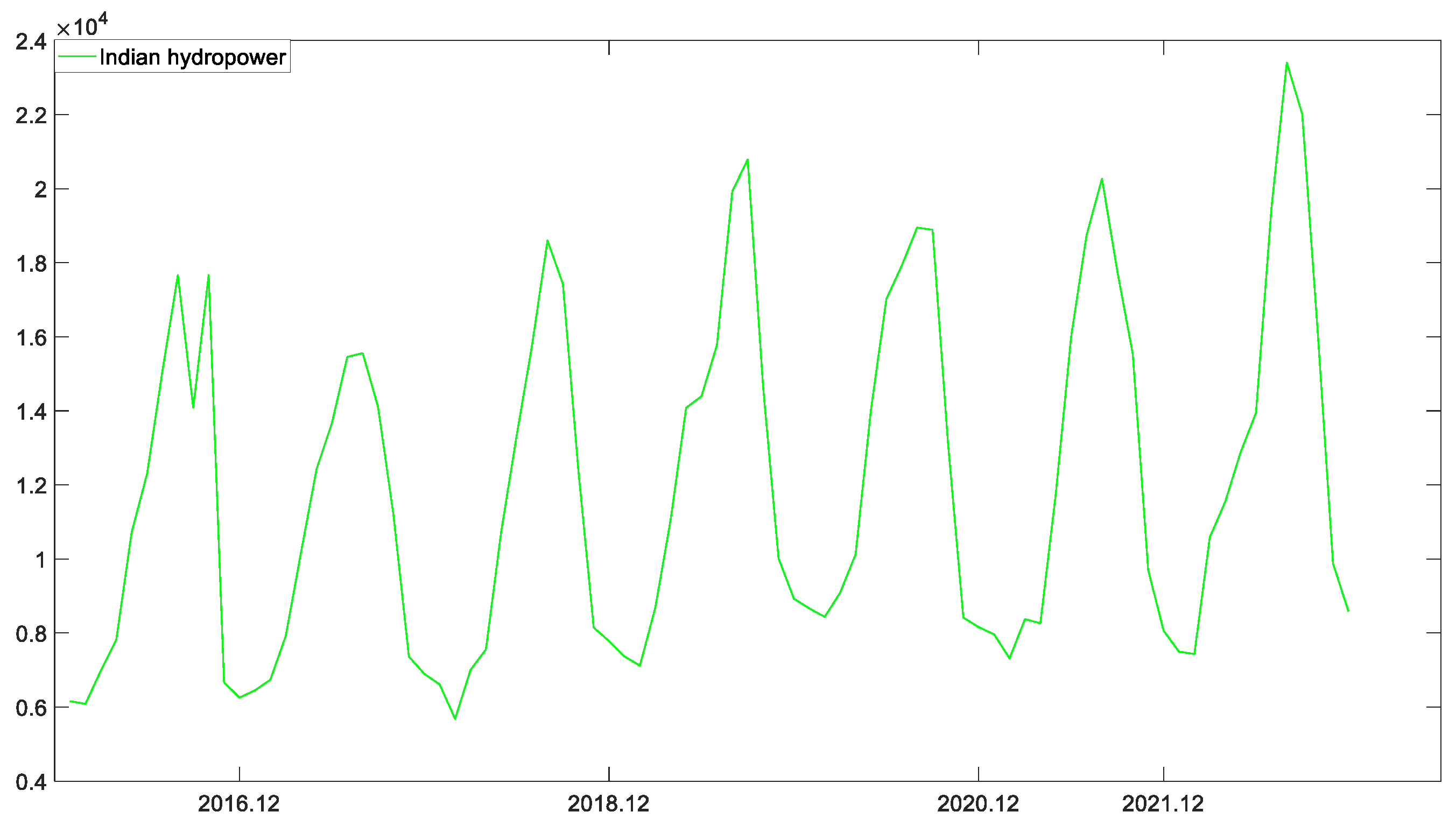
It can be seen from Figure 8 that hydropower generation in India exhibits a stationary development trend and vigorous periodic fluctuation. In order to verify the prediction performance of the newly established model, DPDGSTM(1,1) is employed to predict hydropower generation in India. The visual error comparison and the fitting degree between the predicted value and the original value are, respectively, shown in Figure 9 and Figure 10. Moreover, the detailed prediction results are shown in

Table 5. Prediction results of competing models in the India.

Month	Original	DPDGSTM	APE	DGSM	APE	BPNN	APE	SVR	APE	HW	APE	SARIMA	APE	LSTM	APE
31 January 2022	7497.03	8117.33	7.26	8055.68	7.45	6675.77	10.95	7643.24	1.95	8068.57	7.62	8532.03	13.81	7381.56	1.54
28 February 2022	7433.41	8278.18	5.84	8683.9	16.82	7487.79	0.73	7304.78	1.73	7565.53	1.78	7526.88	1.26	7652.29	2.94
31 March 2022	10,583.82	10,012.31	13.55	9802.29	7.38	7246.41	31.53	8714.85	17.66	8626.3	18.5	8861.31	16.27	8562.48	19.1
30 April 2022	11,540.96	10,766.04	15.13	10,969.36	4.95	7007.95	39.28	10,766.77	6.71	9257.9	19.78	8266.42	28.37	9749.63	15.52
31 May 2022	12,880.91	13,121.07	1.21	14,099.05	9.46	8254.94	35.91	13,463.67	4.52	12,912.66	0.25	12,483.51	3.09	12,482.64	3.09
30 June 2022	13,946.12	16,150.82	18.18	16,266.44	16.64	12,255.46	12.12	16,067.63	15.21	16,342.60	17.18	16,843.04	20.77	15,935.05	14.26
31 July 2022	19,465.11	20317.57	1.17	18,279.48	6.09	17,447.70	10.36	18,387.94	5.53	18,400.66	5.47	18,973.44	2.53	18,848.94	3.17
31 August 2022	23,404.11	23,499.12	9.11	20,321.71	13.17	21,839.10	6.69	20,601.60	11.97	20,112.81	14.06	20,690.50	11.59	20,212.61	13.64
30 September 2022	22,016.56	20,365.77	12.31	19,008.48	13.66	21,839.08	0.81	18,992.32	13.74	18,582.42	15.6	17,852.34	18.91	19,400.14	11.88
31 October 2022	16,178.67	15,910.31	6.31	15,934.23	1.51	15,744.61	2.68	14,431.81	10.8	14,913.19	7.82	15664.05	3.18	15,682.89	3.06
30 November 2022	9880.41	9909.43	1.43	10,231.98	3.56	10,461.36	5.88	10,229.44	3.53	9363.41	5.23	9724.92	1.57	10,040.89	1.62
31 December 2022	8590.76	9898.07	1.88	9532.71	10.96	6682.59	22.21	8255.02	3.91	8202.13	4.52	8093.27	5.79	7863.42	8.47
MAPES		4.5268		7.9154		5.9996		2.1403		10.0413		11.2146		7.3402
RMRSES		0.0545		0.1332		0.0944		0.0296		0.1308		0.1416		0.0933
RMSES		665.0907		1432.6587		1108.7041		415.5744		1546.7905		1782.4593		1019.2247
MAES		530.2588		909.9724		669.3803		260.2304		1158.4274		1366.0236		816.1397
RS		0.9887		0.946		0.9712		0.9959		0.9364		0.9164		0.9719
MAPEP		7.7805		9.3053		14.9304		8.1056		9.818		10.5957		8.1916
RMRSEP		0.0963		0.1047		0.1996		0.0967		0.118		0.1369		0.1021
RMSEP		1445.2064		1599.6646		2368.8878		1592.0963		1846.421		2016.6466		1572.7348
MAEP		1103.4204		1292.8984		1812.1478		1246.4862		1444.455		1496.412		1195.1593
RP		0.969		0.9696		0.9563		0.9693		0.9585		0.9391		0.9697

. As Figure 9 and Table 5 reveal, the SVR achieved the best fitting performance for simulation phase, i.e., MAPES, RMSES, RMRSES, and MAES are significantly smaller than those of other competing models. However, in the prediction stage, various error indicators of the SVR are obviously higher than the new model with a MAPEP of 8.1056%, while the MAPEP of the new model is only 7.7805%. At the same time, combining Figure 10 and Table 5, it can be seen that the new model obtained the minimum MAPEP, RMSEP, RMESEP, and MAEP in the prediction stage, and the comprehensive error evaluation indicators fully demonstrate the superior prediction performance of the new model. Moreover, the LSTM model achieved a better prediction performance in this case, and the error indicators in the prediction stage are just slightly larger than the new model and the SVR. For the SARIMA, HW, and DGSM models, their MAPEP fluctuates on $\left[9.3053\%,10.5957\%\right]$, which can roughly capture the seasonal fluctuation trend of the original sequence, but the predicted value still has a large deviation from the real value at some points. In addition, the BPNN model obtains the highest prediction error, which may be caused by the insufficient sample size, causing it to fall into the problem of overfitting.

4.3.4. Discussion

Combining the above three cases, we can draw the following findings:

(1)

For seasonal series with different sample lengths, development trends, and prediction horizons, the new model always has higher prediction accuracy than the other competing models, which demonstrates that the introduction of a dynamic partial accumulation operator, dummy variables, and time trend item can effectively improve the grey model’s prediction performance for complex fluctuation sequences.

(2)

The grey model DGSM(1,1) can basically fit the development trend of the original series, indicating that the introduction of dummy variables can assist the model in identifying the seasonal fluctuation characteristics of the original series. However, the prediction accuracy of DGSM(1,1) is susceptible to sample length. In the US wind power case with a longer sample, the DGSM(1,1) exhibits a larger prediction deviation.

(3)

The time series models Holt-Winters and SARIMA both have good forecasting performance in the fitting and forecasting stages, especially as the forecasting effect of Holt-Winters is only slightly worse than the new model in many cases, and can be used as a suboptimal replacement model for the new model.

(4)

The machine learning models BPNN, SVR, and LSTM show high fitting accuracy in the three cases. However, they produced significant deviation in the prediction stage which may be caused by the insufficient sample length.

5. Conclusions

In view of the periodicity and complexity of the renewable energy system, this paper constructs a novel dynamic accumulation grey seasonal model which is suitable for mid-to-long-term prediction of renewable energy generation, and the main work and conclusions are summarized as follows:

Firstly, based on the new information priority principle, this paper innovatively puts forward the dynamic partial accumulation operator, which can adaptively select the optimal partial accumulative number according to the sample characteristics. The new method overcomes the problem of the traditional global accumulation technology that it is hard to eliminate old information disturbance and easy to fall into over-accumulation.

Subsequently, given the diverse data characteristics of the renewable energy power generation system, such as upward, downward, and wave trends, this paper integrates a time trend term, dummy variables, and dynamic accumulation operator to identify the periodic and trend variation of the sequence, and establish a novel dynamic partial accumulation grey seasonal model, abbreviated as DPDGSTM(1,1).

Finally, this paper uses three cases to verify the prediction performance of the proposed model. The new model and a series of benchmark models are applied to renewable energy generation prediction in different counties, namely renewable energy power generation in China, wind power generation in the United States, and hydropower generation in India. Based on six evaluation criteria, i.e., APE, MAPE, RMSE, MAE, RMRSE, and R, the prediction accuracy of the new model consistently outperforms other competing models. Hence, the new model is an effective tool for forecasting mid- to- long- term renewable energy generation.

Furthermore, the dynamic partial accumulation operator can also be combined with other models and applied to other fields with periodicity, volatility, and nonlinear characteristics, such as tourism, economy, and environment. However, this study is designed with only a univariate time series, and other exogenous variables that can affect the development of renewable energy systems are not considered, which may limit the prediction performance of the model to some extent. The future work of this study is to further consider the relevant influencing factors that may affect renewable energy generation and construct a multivariate forecasting model to test its modeling effectiveness on renewable energy systems.

References

- Zheng, J.; Du, J.; Wang, B.; Klemes, J.J.; Liao, Q.; Liang, Y. A hybrid framework for forecasting power generation of multiple renewable energy sources. Renew. Sustain. Energy Rev. 2023, 172, 113046. [Google Scholar] [CrossRef]
- Lledó, L.; Ramon, J.; Soret, A.; Doblas-Reyes, F. Seasonal prediction of renewable energy generation in Europe based on four teleconnection indices. Renew. Energy 2022, 186, 420–430. [Google Scholar] [CrossRef]
- Hoseinzadeh, S.; Garcia, D.A. Techno-economic assessment of hybrid energy flexibility systems for islands’ decarbonization: A case study in Italy. Sustain. Energy Technol. Assess. 2022, 51, 101929. [Google Scholar] [CrossRef]
- Ye, L.; Zhao, Y.; Zeng, C.; Zhang, C. Short-term wind power prediction based on spatial model. Renew. Energy 2017, 101, 1067–1074. [Google Scholar] [CrossRef]
- Wang, H.; Han, S.; Liu, Y.; Yan, J.; Li, L. Sequence transfer correction algorithm for numerical weather prediction wind speed and its application in a wind power forecasting system. Appl. Energy 2019, 237, 1–10. [Google Scholar] [CrossRef]
- Hoseinzadeh, S.; Ghasemi, M.H.; Heyns, S. Application of hybrid systems in solution of low power generation at hot seasons for micro hydro systems. Renew. Energy 2020, 160, 323–332. [Google Scholar] [CrossRef]
- Singh, S.N.; Mohapatra, A. Repeated wavelet transform based ARIMA model for very short-term wind speed forecasting. Renew. Energy 2019, 136, 758–768. [Google Scholar]
- Kushwaha, V.; Pindoriya, N.M. A SARIMA-RVFL hybrid model assisted by wavelet decomposition for very short-term solar PV power generation forecast. Renew. Energy 2019, 140, 124–139. [Google Scholar] [CrossRef]
- Ziel, F.; Croonenbroeck, C.; Ambach, D. Forecasting wind power–modeling periodic and non-linear effects under conditional heteroscedasticity. Appl. Energy 2016, 177, 285–297. [Google Scholar] [CrossRef] [Green Version]
- Jamil, R. Hydroelectricity consumption forecast for Pakistan using ARIMA modeling and supply-demand analysis for the year 2030. Renew. Energy 2020, 154, 1–10. [Google Scholar] [CrossRef]
- Alsharif, M.H.; Younes, M.K.; Kim, J. Time series ARIMA model for prediction of daily and monthly average global solar radiation: The case study of Seoul, South Korea. Symmetry 2019, 11, 240. [Google Scholar] [CrossRef] [Green Version]
- Wang, F.; Zhen, Z.; Wang, B.; Mi, Z. Comparative study on KNN and SVM based weather classification models for day ahead short term solar PV power forecasting. Appl. Sci. 2017, 8, 28. [Google Scholar] [CrossRef] [Green Version]
- Liu, M.D.; Ding, L.; Bai, Y.L. Application of hybrid model based on empirical mode decomposition, novel recurrent neural networks and the ARIMA to wind speed prediction. Energy Convers. Manag. 2021, 233, 113917. [Google Scholar] [CrossRef]
- Zhang, W.; Lin, Z.; Liu, X. Short-term offshore wind power forecasting-A hybrid model based on Discrete Wavelet Transform (DWT), Seasonal Autoregressive Integrated Moving Average (SARIMA), and deep-learning-based Long Short-Term Memory (LSTM). Renew. Energy 2022, 185, 611–628. [Google Scholar] [CrossRef]
- Dash, D.R.; Dash, P.K.; Bisoi, R. Short term solar power forecasting using hybrid minimum variance expanded RVFLN and Sine-Cosine Levy Flight PSO algorithm. Renew. Energy 2021, 174, 513–537. [Google Scholar] [CrossRef]
- Khan, Z.A.; Hussain, T.; Ul Haq, I.; Ullah, F.M.; Baik, S. Towards efficient and effective renewable energy prediction via deep learning. Energy Rep. 2022, 8, 10230–10243. [Google Scholar] [CrossRef]
- Wang, B.; Li, Y.; Huang, G.; Gao, P.; Liu, J.; Wen, Y. Development of an integrated BLSVM-MFA method for analyzing renewable power-generation potential under climate change: A case study of Xiamen. Appl. Energy 2023, 337, 120888. [Google Scholar] [CrossRef]
- Ding, S.; Zhang, H.; Tao, Z.; Li, R. Integrating data decomposition and machine learning methods: An empirical proposition and analysis for renewable energy generation forecasting. Expert Syst. Appl. 2022, 204, 117635. [Google Scholar] [CrossRef]
- Luo, D.; Wang, X.L.; Sun, D.C.; Zhang, G.Z. Discrete grey DGM(1,1,T) model with time periodic term and its application. Syst. Eng. Theory Pract. 2020, 40, 2737–2746. [Google Scholar]
- Song, Z.M.; Deng, J.L. The accumulated generating operation in opposite direction and its use in grey model GOM(1,1). Syst. Eng. 2001, 19, 66–69. [Google Scholar]
- Xia, M.; Wong, W.K. A seasonal discrete grey forecasting model for fashion retailing. Knowl. Based Syst. 2014, 57, 119–126. [Google Scholar] [CrossRef]
- Wu, L.F.; Liu, S.F.; Liu, J. GM(1,1) model based on fractional order accumulating method and its stability. Control Decis. 2014, 29, 919–924. [Google Scholar]
- Zhou, W.J.; Zhang, H.R.; Dang, Y.G.; Wang, Z.X. New information priority accumulated grey discrete model and its application. Chin. J. Manag. Sci. 2017, 25, 140–148. [Google Scholar]
- Xiao, X.P.; Liu, J.; Guo, H. Properties and optimization of generalized accumulation grey model. Syst. Eng. Theory Pract. 2014, 34, 1547–1556. [Google Scholar]
- Wu, L.F.; Fu, B. GM(1,1) model with fractional order opposite-direction accumulated generation and its properties. Stat. Decis. 2017, 18, 33–36. [Google Scholar]
- Zhou, W.; Ding, S. A novel discrete grey seasonal model and its applications. Commun. Nonlinear Sci. Numer. Simul. 2021, 93, 105493. [Google Scholar] [CrossRef]
- Zhou, W.; Wu, X.; Ding, S.; Chen, Y. Predictive analysis of the air quality indicators in the Yangtze River Delta in China: An application of a novel seasonal grey model. Sci. Total Environ. 2020, 748, 141428. [Google Scholar] [CrossRef]
- Wang, J.Z.; Ma, X.; Wu, J.; Dong, Y. Optimization models based on GM (1,1) and seasonal fluctuation for electricity demand forecasting. Int. J. Electr. Power Energy Syst. 2012, 43, 109–117. [Google Scholar] [CrossRef]
- Zhou, W.; Jiang, R.; Ding, S.; Chen, Y.; Yao, L.; Tao, H. A novel grey prediction model for seasonal time series. Knowl. Based Syst. 2021, 229, 107363. [Google Scholar] [CrossRef]
- Wang, Z.X.; Li, Q.; Pei, L. A seasonal GM(1,1) model for forecasting the electricity consumption of the primary economic sectors. Energy 2018, 154, 522–534. [Google Scholar] [CrossRef]
- Ding, S.; Tao, Z.; Li, R.; Qin, X. A novel seasonal adaptive grey model with the data-restacking technique for monthly renewable energy consumption forecasting. Expert Syst. Appl. 2022, 208, 118115. [Google Scholar] [CrossRef]
- Qian, W.; Sui, A. A novel structural adaptive discrete grey prediction model and its application in forecasting renewable energy generation. Expert Syst. Appl. 2021, 186, 115761. [Google Scholar] [CrossRef]
- Wang, Y.; Yang, Z.; Wang, L.; Ma, X.; Wu, W.; Ye, L.; Zhou, Y.; Luo, Y. Forecasting China’s energy production and consumption based on a novel structural adaptive Caputo fractional grey prediction model. Energy 2022, 259, 124935. [Google Scholar] [CrossRef]
- He, X.; Wang, Y.; Zhang, Y.; Ma, X.; Wu, W.; Zhang, L. A novel structure adaptive new information priority discrete grey prediction model and its application in renewable energy generation forecasting. Appl. Energy 2022, 325, 119854. [Google Scholar] [CrossRef]
Figure 1.
The flowchart of modeling process and parameter solution.
Figure 2.
Renewable energy generation in China from 2016 to 2022.
Figure 3.
Visual errors comparison of the competing models in China.
Figure 4.
Comparison of the predicted values of the competing models in China.
Figure 5.
Wind power in America from 2001 to 2022.
Figure 6.
Visual errors comparison of the competing models in United States.
Figure 7.
Comparison of the predicted values of the competing models in the United States.
Figure 8.
Hydropower generation in India from 2016 to 2022.
Figure 9.
Visual errors comparison of the competing models in India.
Figure 10.
Comparison of the predicted values of the competing models in India.