
Novel Approach to Predicting Soil Permeability Coefficient Using Gaussian Process Regression

 ,
,  , and
, and
Abstract
:1. Introduction
2. Methodology
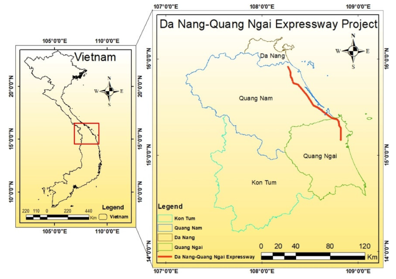
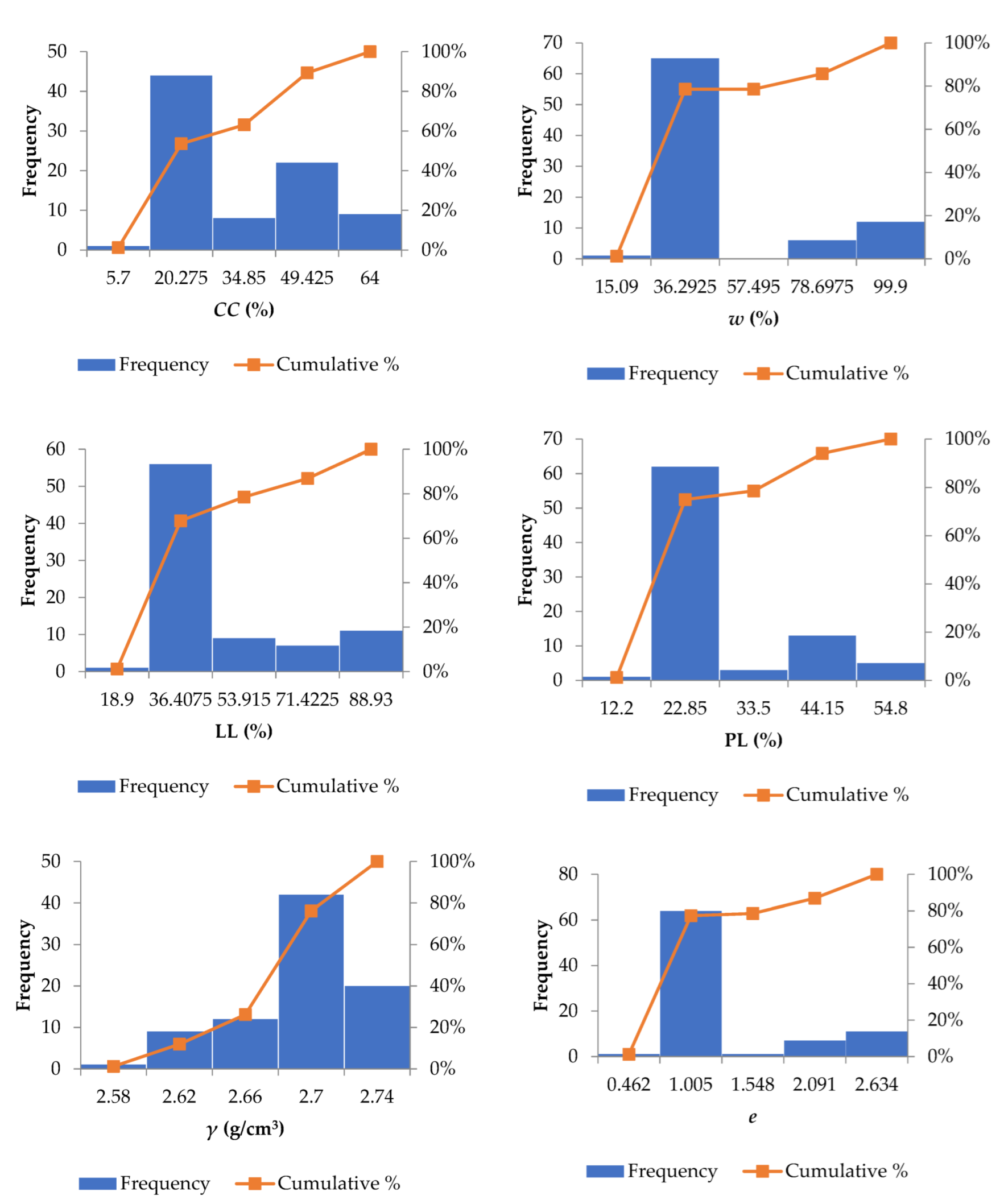
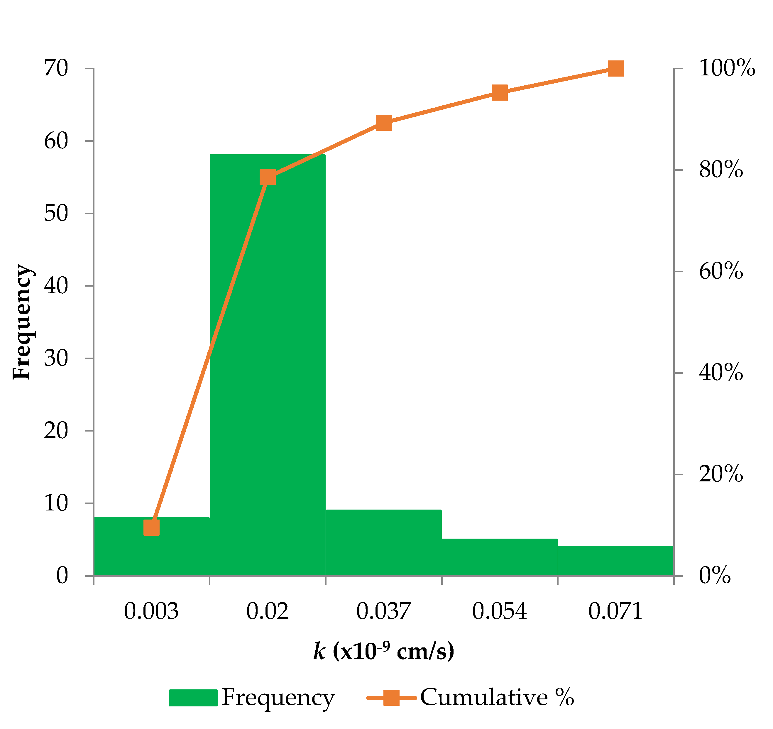
2.1. Data Catalog
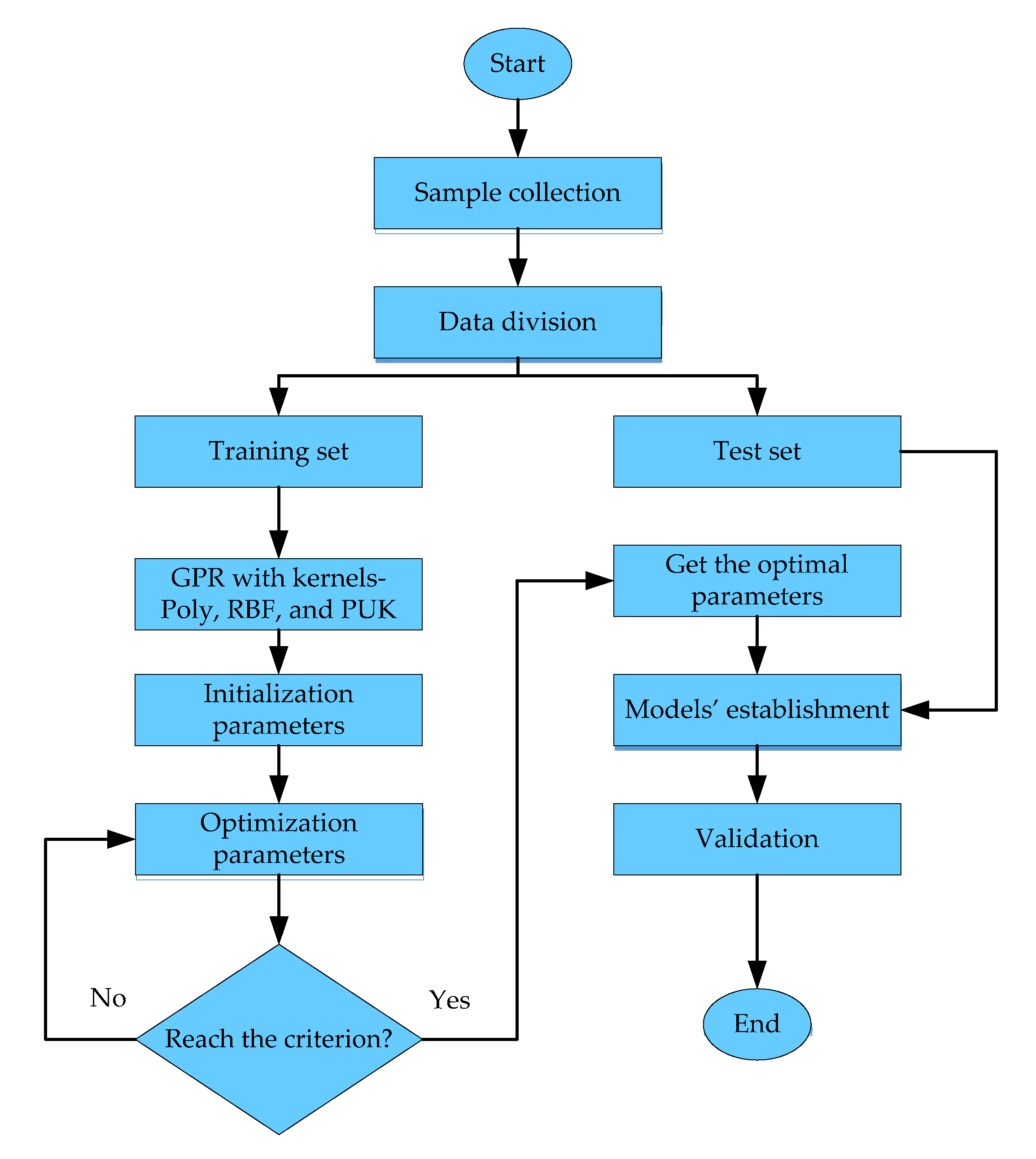
2.2. Gaussian Process Regression
Details of Kernel Functions
- Polynomial (Poly)
- 2.
- Radial basis function (RBF)
- 3.
- Pearson universal kernel (PUK)
2.3. Performance Metrics and Evaluation
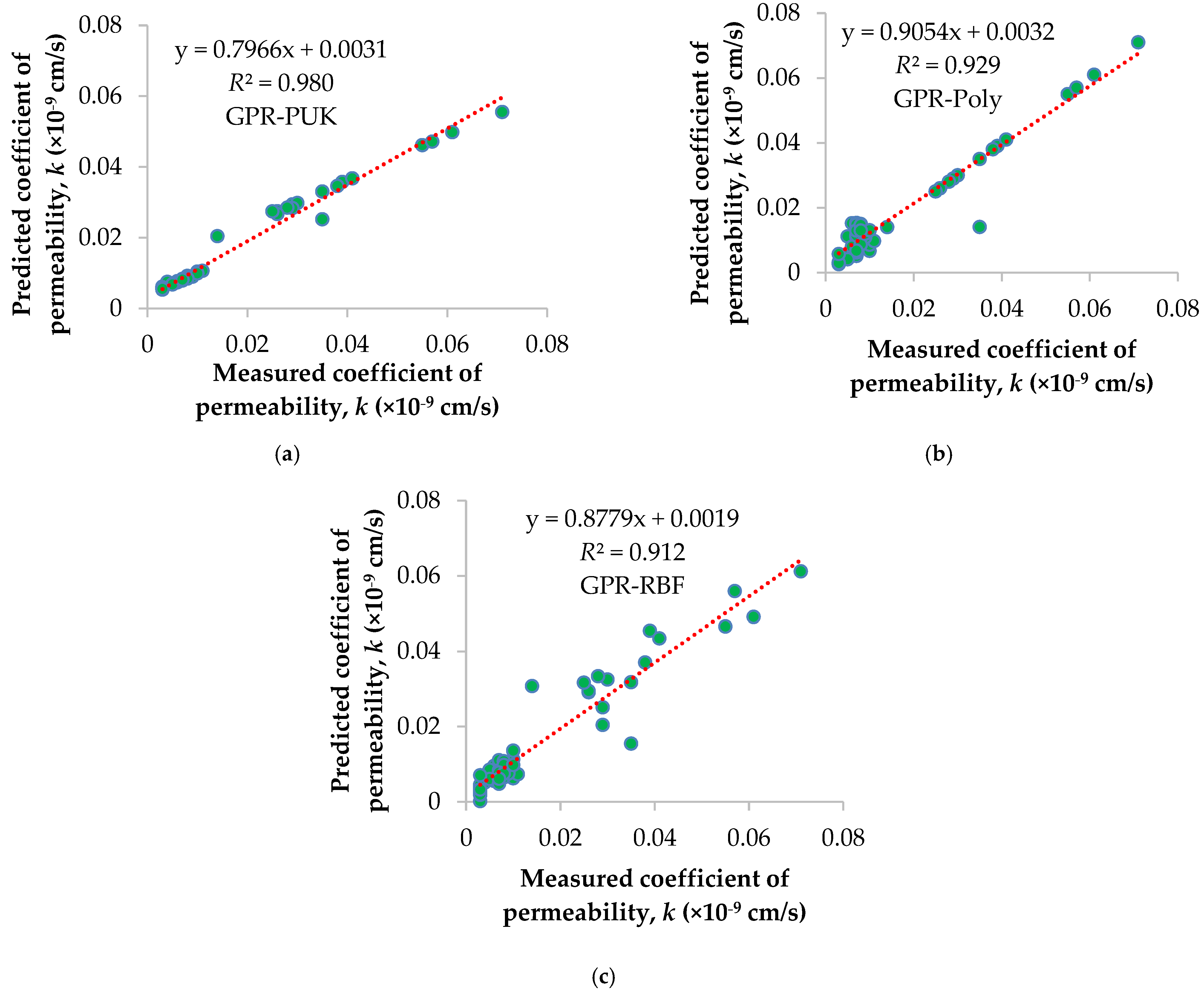
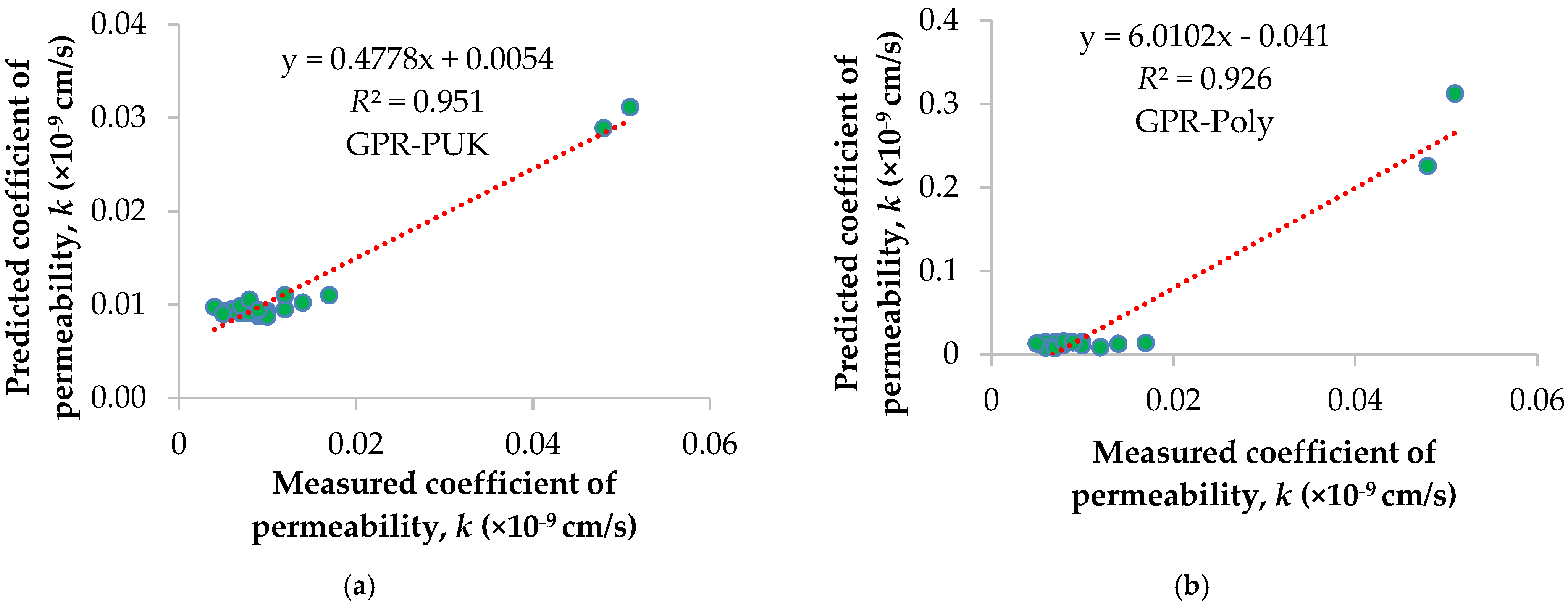
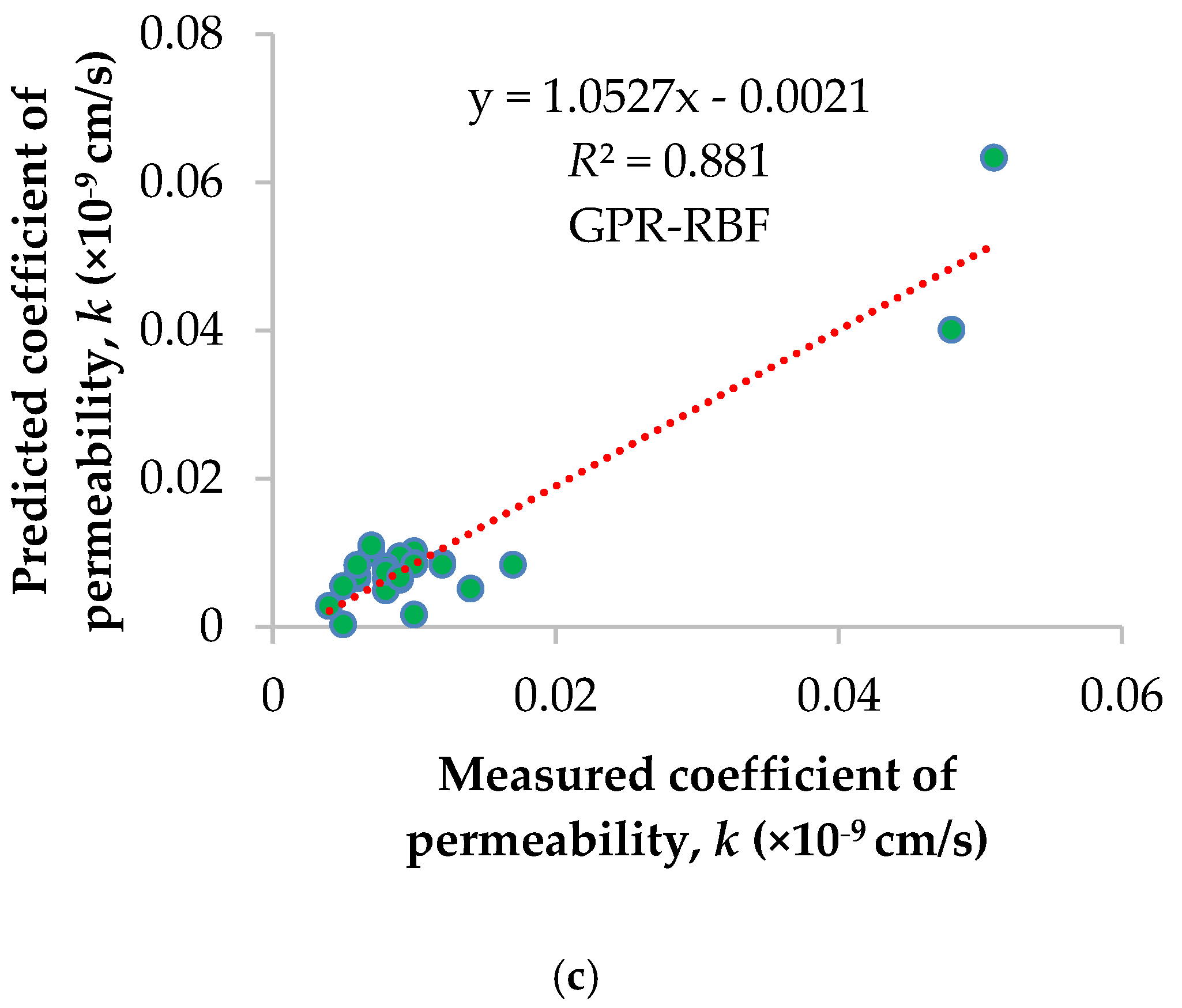
3. Results and Discussion
4. Comparison of Performance with Other Methods
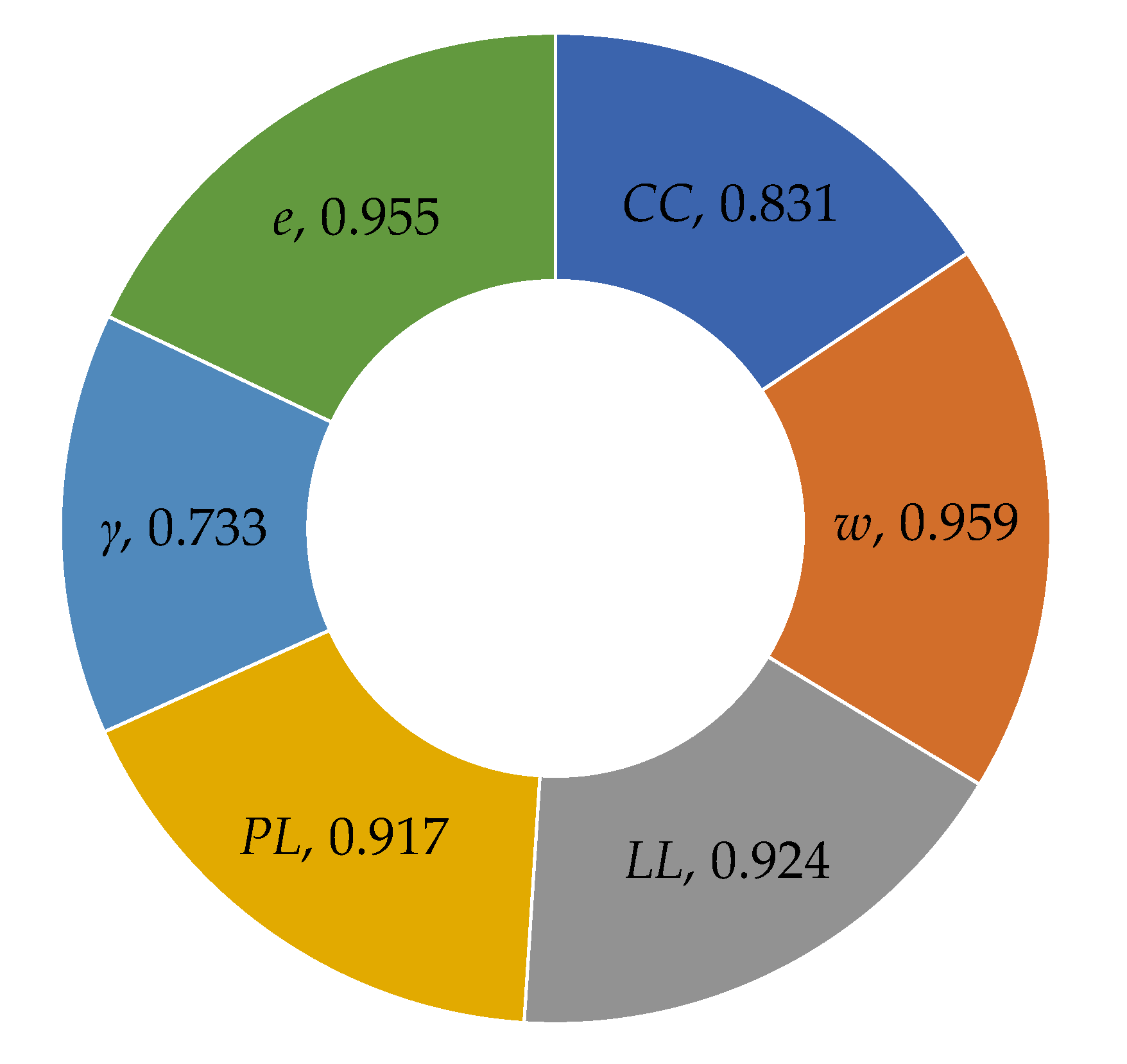
5. Sensitivity Analysis
6. Conclusions
- Comparing GPR models’ performance reveals that the GPR-PUK model gives more accurate prediction results with the coefficient of determination being 0.951, achieved from the correlation between experimental and estimated values of k.
- The GPR-PUK model’s estimation of the soil permeability coefficient was found to be more reliable than that of the ANN, SVM, RF, and M5P models reported in the literature.
- The findings of the sensitivity analysis demonstrate that different input factors have varying degrees of significance on the coefficient of soil permeability as w > e > LL > PL > CC > γ.
Author Contributions
Funding
Institutional Review Board Statement
Informed Consent Statement
Data Availability Statement
Acknowledgments
Conflicts of Interest
Notation
| ANN | Artificial neural network |
| RF | Random forest |
| SVM | Support vector machine |
| GPR | Gaussian process regression |
| MAE | Mean absolute error |
| M5P | M5Prime algorithm |
| RMSE | Root mean square error |
| PUK | Pearson universal kernel |
| RBF | Radial basis function |
| XGBoost | Extreme gradient boosting |
| R2 | Coefficient of determination |
| R | Correlation coefficient |
| k | Soil permeability coefficient (×10−9 cm/s) |
| LL | Liquid limit (%) |
| PL | Plastic limit (%) |
| CC | Clay content (%) |
| e | Void ratio |
| w | Natural water content (%) |
| γ | Specific density (g/cm3) |
Appendix A

| S. No. | CC (%) | w (%) | LL (%) | PL (%) | γ (g/cm3) | e | k (×10−9 cm/s) |
|---|---|---|---|---|---|---|---|
| 1 | 44 | 93.73 | 75.62 | 46.8 | 2.59 | 2.453 | 0.029 |
| 2 | 21.7 | 20.71 | 24.58 | 13.5 | 2.72 | 0.639 | 0.01 |
| 3 | 51.8 | 20.98 | 38.17 | 20.2 | 2.73 | 0.625 | 0.003 |
| 4 | 9.7 | 18.02 | 20.51 | 14.2 | 2.68 | 0.605 | 0.007 |
| 5 | 46.9 | 95.58 | 82.25 | 53 | 2.6 | 2.514 | 0.026 |
| 6 | 12.7 | 22.71 | 28.5 | 17.8 | 2.69 | 0.671 | 0.01 |
| 7 | 47.5 | 85.35 | 71.24 | 40.5 | 2.62 | 2.275 | 0.014 |
| 8 | 59.4 | 24.95 | 41.87 | 22.3 | 2.74 | 0.713 | 0.003 |
| 9 | 9.2 | 23.97 | 26.52 | 19.8 | 2.67 | 0.723 | 0.008 |
| 10 | 55.3 | 98.01 | 73.63 | 40.1 | 2.59 | 2.597 | 0.035 |
| 11 | 44.8 | 79.96 | 75.45 | 43.6 | 2.59 | 2.083 | 0.039 |
| 12 | 51.1 | 73.75 | 66.96 | 35.8 | 2.61 | 1.966 | 0.061 |
| 13 | 46.1 | 25.78 | 38.03 | 17.5 | 2.73 | 0.808 | 0.003 |
| 14 | 56.1 | 83.25 | 78.23 | 41.9 | 2.62 | 2.235 | 0.055 |
| 15 | 16.1 | 17.52 | 25.85 | 12.2 | 2.69 | 0.546 | 0.01 |
| 16 | 49 | 25.45 | 48.24 | 24.8 | 2.72 | 0.711 | 0.003 |
| 17 | 10.7 | 24.53 | 27.22 | 19.6 | 2.69 | 0.713 | 0.007 |
| 18 | 64 | 78.72 | 75.53 | 39.5 | 2.64 | 2.106 | 0.03 |
| 19 | 5.7 | 17.35 | 20.34 | 14.25 | 2.66 | 0.494 | 0.006 |
| 20 | 41.9 | 69.26 | 66.42 | 48.5 | 2.64 | 1.87 | 0.029 |
| 21 | 9.5 | 18.12 | 21.2 | 14.5 | 2.68 | 0.567 | 0.008 |
| 22 | 7.6 | 20.23 | 23.62 | 16.8 | 2.69 | 0.64 | 0.007 |
| 23 | 11 | 20.14 | 22.78 | 16.1 | 2.67 | 0.608 | 0.008 |
| 24 | 45 | 35.53 | 53.56 | 28.6 | 2.74 | 1.015 | 0.004 |
| 25 | 8.5 | 20.81 | 25.31 | 18.53 | 2.68 | 0.576 | 0.005 |
| 26 | 8.6 | 20.12 | 20.82 | 14.8 | 2.67 | 0.599 | 0.007 |
| 27 | 10.7 | 17.25 | 19.5 | 13.5 | 2.68 | 0.558 | 0.008 |
| 28 | 8.9 | 21.79 | 24.98 | 19 | 2.68 | 0.654 | 0.007 |
| 29 | 46.4 | 99.9 | 82.11 | 43.6 | 2.58 | 2.634 | 0.041 |
| 30 | 9.7 | 17.34 | 20.49 | 14.3 | 2.66 | 0.486 | 0.007 |
| 31 | 25.9 | 21.23 | 31.18 | 13.2 | 2.72 | 0.609 | 0.005 |
| 32 | 12.5 | 19.25 | 23.46 | 14.67 | 2.67 | 0.628 | 0.008 |
| 33 | 8.4 | 19.46 | 22.97 | 17.43 | 2.68 | 0.605 | 0.007 |
| 34 | 8.1 | 23.28 | 26.8 | 20.36 | 2.68 | 0.707 | 0.011 |
| 35 | 23.6 | 18.84 | 27.48 | 13.8 | 2.71 | 0.604 | 0.006 |
| 36 | 63.4 | 73.1 | 68.47 | 35 | 2.61 | 1.933 | 0.028 |
| 37 | 19 | 18.35 | 23.61 | 13.35 | 2.7 | 0.579 | 0.007 |
| 38 | 42.5 | 27.28 | 39.99 | 21.74 | 2.72 | 0.789 | 0.003 |
| 39 | 49.4 | 62.2 | 59.99 | 38.5 | 2.63 | 1.657 | 0.026 |
| 40 | 23.5 | 21.32 | 32.23 | 16.4 | 2.71 | 0.604 | 0.005 |
| 41 | 6.1 | 16.97 | 21.01 | 15.87 | 2.66 | 0.556 | 0.007 |
| 42 | 7.7 | 21.23 | 25.3 | 18.5 | 2.68 | 0.654 | 0.009 |
| 43 | 9.7 | 18.01 | 20.3 | 14.2 | 2.67 | 0.599 | 0.007 |
| 44 | 8.5 | 25.49 | 27.49 | 21.32 | 2.67 | 0.723 | 0.008 |
| 45 | 60.2 | 95.09 | 84.05 | 54.8 | 2.63 | 2.507 | 0.038 |
| 46 | 40.3 | 20.75 | 40.77 | 18.64 | 2.72 | 0.591 | 0.003 |
| 47 | 8.4 | 18.25 | 21.08 | 14.5 | 2.69 | 0.592 | 0.008 |
| 48 | 50.7 | 28.97 | 46.04 | 25.2 | 2.72 | 0.889 | 0.003 |
| 49 | 8.8 | 17.19 | 19.81 | 14.3 | 2.68 | 0.549 | 0.007 |
| 50 | 46.6 | 76.77 | 64.83 | 38.17 | 2.63 | 2.023 | 0.025 |
| 51 | 9.6 | 17.99 | 20.42 | 15 | 2.67 | 0.571 | 0.008 |
| 52 | 8.6 | 19.9 | 23 | 16.9 | 2.68 | 0.586 | 0.009 |
| 53 | 9.2 | 17.81 | 21 | 14.3 | 2.68 | 0.506 | 0.01 |
| 54 | 11.7 | 19.77 | 23.91 | 13.5 | 2.68 | 0.567 | 0.035 |
| 55 | 9.4 | 17.85 | 20.48 | 14.8 | 2.68 | 0.558 | 0.008 |
| 56 | 45.1 | 93.19 | 88.93 | 48 | 2.62 | 2.447 | 0.057 |
| 57 | 46.1 | 70.21 | 65.46 | 33.6 | 2.64 | 1.87 | 0.071 |
| 58 | 37.4 | 21.13 | 32.44 | 14.2 | 2.71 | 0.642 | 0.003 |
| 59 | 45.3 | 19.6 | 30.92 | 13.2 | 2.73 | 0.569 | 0.007 |
| 60 | 19 | 24.55 | 29.08 | 19.6 | 2.68 | 0.707 | 0.017 |
| 61 | 37.6 | 87.71 | 75.34 | 40.5 | 2.63 | 2.329 | 0.048 |
| 62 | 8 | 18.05 | 20.99 | 14.3 | 2.68 | 0.595 | 0.01 |
| 63 | 8.5 | 19.85 | 23.67 | 17.58 | 2.67 | 0.599 | 0.008 |
| 64 | 9.6 | 18.18 | 22.58 | 16 | 2.68 | 0.567 | 0.006 |
| 65 | 8.6 | 18.02 | 20.51 | 14.6 | 2.69 | 0.592 | 0.012 |
| 66 | 8.3 | 18.01 | 21 | 14.2 | 2.67 | 0.599 | 0.007 |
| 67 | 10.2 | 18.15 | 22.14 | 15.6 | 2.67 | 0.517 | 0.006 |
| 68 | 8.6 | 24.84 | 29.32 | 22 | 2.68 | 0.752 | 0.012 |
| 69 | 45.8 | 89.51 | 85.86 | 42.7 | 2.63 | 2.372 | 0.051 |
| 70 | 38.6 | 22.79 | 35.83 | 15.2 | 2.72 | 0.689 | 0.009 |
| 71 | 8.2 | 17.12 | 19.7 | 13.8 | 2.67 | 0.571 | 0.01 |
| 72 | 26.5 | 21.89 | 30.98 | 17.4 | 2.72 | 0.619 | 0.005 |
| 73 | 24.5 | 18.28 | 28.11 | 12.5 | 2.71 | 0.522 | 0.006 |
| 74 | 21 | 20.62 | 28.62 | 17.4 | 2.69 | 0.592 | 0.014 |
| 75 | 9.3 | 21.14 | 23.89 | 18.53 | 2.68 | 0.686 | 0.008 |
| 76 | 8.4 | 18.02 | 21.1 | 14.5 | 2.67 | 0.552 | 0.009 |
| 77 | 9.8 | 18.07 | 20.62 | 14.5 | 2.68 | 0.567 | 0.01 |
| 78 | 30.4 | 22.23 | 39.53 | 18.64 | 2.72 | 0.648 | 0.004 |
| 79 | 9.8 | 22.03 | 23.92 | 17.8 | 2.68 | 0.644 | 0.008 |
| 80 | 6.7 | 18.91 | 21.49 | 15 | 2.69 | 0.582 | 0.007 |
| 81 | 43.4 | 25.6 | 34.5 | 15.6 | 2.73 | 0.717 | 0.005 |
| 82 | 40.1 | 25.53 | 36.11 | 19.2 | 2.72 | 0.755 | 0.01 |
| 83 | 8.7 | 15.09 | 18.9 | 12.63 | 2.66 | 0.462 | 0.008 |
| 84 | 9.4 | 19.64 | 23.8 | 17.2 | 2.67 | 0.648 | 0.009 |
References
- Pham, B.T.; Nguyen, M.D.; Al-Ansari, N.; Tran, Q.A.; Ho, L.S.; Le, H.V.; Prakash, I. A Comparative Study of Soft Computing Models for Prediction of Permeability Coefficient of Soil. Math. Probl. Eng. 2021, 2021, 7631493. [Google Scholar] [CrossRef]
- Ganjidoost, H.; Mousavi, S.J.; Soroush, A. Adaptive network-based fuzzy inference systems coupled with genetic algorithms for predicting soil permeability coefficient. Neural Process. Lett. 2016, 44, 53–79. [Google Scholar] [CrossRef]
- Cedergren, H.R. Seepage, Drainage, and Flow Nets; Wiley: London, UK, 1988; Volume 3. [Google Scholar]
- Shakoor, A.; Cook, B.D. The effect of stone content, size, and shape on the engineering properties of a compacted silty clay. Bull. Assoc. Eng. Geol. 1990, 27, 245–253. [Google Scholar] [CrossRef]
- Mitchell, J.K.; Hooper, D.R.; Campenella, R.G. Permeability of compacted clay. J. Soil Mech. Found. Div. 1965, 91, 41–65. [Google Scholar] [CrossRef]
- Olson, R.E. Effective stress theory of soil compaction. J. Soil Mech. Found. Div. 1963, 89, 27–45. [Google Scholar] [CrossRef]
- Vienken, T.; Dietrich, P. Field evaluation of methods for determining hydraulic conductivity from grain size data. J. Hydrol. 2011, 400, 58–71. [Google Scholar] [CrossRef]
- Rehfeldt, K.R.; Boggs, J.M.; Gelhar, L.W. Field study of dispersion in a heterogeneous aquifer: 3. Geostatistical analysis of hydraulic conductivity. Water Resour. Res. 1992, 28, 3309–3324. [Google Scholar] [CrossRef]
- Sinha, S.K.; Wang, M.C. Artificial neural network prediction models for soil compaction and permeability. Geotech. Geol. Eng. 2008, 26, 47–64. [Google Scholar] [CrossRef]
- Elhakim, A.F. Estimation of soil permeability. Alex. Eng. J. 2016, 55, 2631–2638. [Google Scholar] [CrossRef] [Green Version]
- Rawls, W.; Brakensiek, D. Estimation of soil water retention and hydraulic properties. In Unsaturated Flow in Hydrologic Modeling; Springer: Berlin/Heidelberg, Germany, 1989; pp. 275–300. [Google Scholar]
- Sperry, J.M.; Peirce, J.J. A model for estimating the hydraulic conductivity of granular material based on grain shape, grain size, and porosity. Groundwater 1995, 33, 892–898. [Google Scholar] [CrossRef]
- Lebron, I.; Schaap, M.; Suarez, D. Saturated hydraulic conductivity prediction from microscopic pore geometry measurements and neural network analysis. Water Resour. Res. 1999, 35, 3149–3158. [Google Scholar] [CrossRef]
- Hauser, V.L. Seepage control by particle size selection. Trans. ASAE 1978, 21, 691–0695. [Google Scholar] [CrossRef]
- Froemelt, A.; Dürrenmatt, D.J.; Hellweg, S. Using data mining to assess environmental impacts of household consumption behaviors. Environ. Sci. Technol. 2018, 52, 8467–8478. [Google Scholar] [CrossRef] [PubMed]
- Ahmad, M.; Tang, X.-W.; Qiu, J.-N.; Gu, W.-J.; Ahmad, F. A hybrid approach for evaluating CPT-based seismic soil liquefaction potential using Bayesian belief networks. J. Cent. South Univ. 2020, 27, 500–516. [Google Scholar]
- Ahmad, M.; Tang, X.-W.; Qiu, J.-N.; Ahmad, F. Evaluating Seismic Soil Liquefaction Potential Using Bayesian Belief Network and C4. 5 Decision Tree Approaches. Appl. Sci. 2019, 9, 4226. [Google Scholar] [CrossRef] [Green Version]
- Ahmad, M.; Tang, X.; Qiu, J.; Ahmad, F.; Gu, W. LLDV-a Comprehensive Framework for Assessing the Effects of Liquefaction Land Damage Potential. In Proceedings of the 2019 IEEE 14th International Conference on Intelligent Systems and Knowledge Engineering (ISKE), Dalian, China, 14–16 November 2019; pp. 527–533. [Google Scholar]
- Ahmad, M.; Tang, X.-W.; Qiu, J.-N.; Ahmad, F.; Gu, W.-J. A step forward towards a comprehensive framework for assessing liquefaction land damage vulnerability: Exploration from historical data. Front. Struct. Civ. Eng. 2020, 14, 1476–1491. [Google Scholar] [CrossRef]
- Ahmad, M.; Tang, X.; Ahmad, F. Evaluation of Liquefaction-Induced Settlement Using Random Forest and REP Tree Models: Taking Pohang Earthquake as a Case of Illustration. In Natural Hazards-Impacts, Adjustments & Resilience; IntechOpen: London, UK, 2020. [Google Scholar]
- Ahmad, M.; Al-Shayea, N.A.; Tang, X.-W.; Jamal, A.; Al-Ahmadi, H.M.; Ahmad, F. Predicting the Pillar Stability of Underground Mines with Random Trees and C4. 5 Decision Trees. Appl. Sci. 2020, 10, 6486. [Google Scholar] [CrossRef]
- Yilmaz, I.; Marschalko, M.; Bednarik, M.; Kaynar, O.; Fojtova, L. Neural computing models for prediction of permeability coefficient of coarse-grained soils. Neural Comput. Appl. 2012, 21, 957–968. [Google Scholar] [CrossRef]
- Park, H. Development of neural network model to estimate the permeability coefficient of soils. Mar. Georesources Geotechnol. 2011, 29, 267–278. [Google Scholar] [CrossRef]
- Sezer, A.; Göktepe, A.B.; Altun, S. Estimation of the Permeability of Granular Soils Using Neuro-fuzzy System. In Proceedings of the AIAI Workshops, Thessaloniki, Greece, 23–25 April 2009; pp. 333–342. [Google Scholar]
- Pham, B.T.; Qi, C.; Ho, L.S.; Nguyen-Thoi, T.; Al-Ansari, N.; Nguyen, M.D.; Nguyen, H.D.; Ly, H.-B.; Le, H.V.; Prakash, I. A novel hybrid soft computing model using random forest and particle swarm optimization for estimation of undrained shear strength of soil. Sustainability 2020, 12, 2218. [Google Scholar] [CrossRef] [Green Version]
- Singh, V.K.; Kumar, D.; Kashyap, P.; Singh, P.K.; Kumar, A.; Singh, S.K. Modelling of soil permeability using different data driven algorithms based on physical properties of soil. J. Hydrol. 2020, 580, 124223. [Google Scholar] [CrossRef]
- Garcia-Bengochea, I.; Altschaeffl, A.G.; Lovell, C.W. Pore distribution and permeability of silty clays. J. Geotech. Eng. Div. 1979, 105, 839–856. [Google Scholar] [CrossRef]
- Pham, B.T.; Ly, H.-B.; Al-Ansari, N.; Ho, L.S. A Comparison of Gaussian Process and M5P for Prediction of Soil Permeability Coefficient. Sci. Program. 2021, 2021, 3625289. [Google Scholar] [CrossRef]
- Pham, T.A.; Tran, V.Q.; Vu, H.-L.T.; Ly, H.-B. Design deep neural network architecture using a genetic algorithm for estimation of pile bearing capacity. PLoS ONE 2020, 15, e0243030. [Google Scholar] [CrossRef] [PubMed]
- Liang, W.; Luo, S.; Zhao, G.; Wu, H. Predicting hard rock pillar stability using GBDT, XGBoost, and LightGBM algorithms. Mathematics 2020, 8, 765. [Google Scholar] [CrossRef]
- Ahmad, M.H.; Hu, J.-L.; Ahmad, F.; Tang, X.-W.; Amjad, M.; Iqbal, M.J.; Asim, M.; Farooq, A. Supervised Learning Methods for Modeling Concrete Compressive Strength Prediction at High Temperature. Materials 2021, 14, 1983. [Google Scholar] [CrossRef] [PubMed]
- Rasmussen, C.; Williams, C. Gaussian Processes for Machine Learning; The MIT Press: Cambridge, MA, USA, 2006; Volume 38, pp. 715–719. [Google Scholar]
- Kuss, M. Gaussian Process Models for Robust Regression, Classification, and Reinforcement Learning. Ph.D. Thesis, Echnische Universität Darmstadt Darmstadt, Darmstadt, Germany, 2006. [Google Scholar]
- Ahmad, M.; Amjad, M.; Al-Mansob, R.A.; Kamiński, P.; Olczak, P.; Khan, B.J.; Alguno, A.C. Prediction of Liquefaction-Induced Lateral Displacements Using Gaussian Process Regression. Appl. Sci. 2022, 12, 1977. [Google Scholar] [CrossRef]
- Sihag, P.; Tiwari, N.; Ranjan, S. Modelling of infiltration of sandy soil using gaussian process regression. Modeling Earth Syst. Environ. 2017, 3, 1091–1100. [Google Scholar] [CrossRef]
- Elbeltagi, A.; Azad, N.; Arshad, A.; Mohammed, S.; Mokhtar, A.; Pande, C.; Etedali, H.R.; Bhat, S.A.; Islam, A.R.M.T.; Deng, J. Applications of Gaussian process regression for predicting blue water footprint: Case study in Ad Daqahliyah, Egypt. Agric. Water Manag. 2021, 255, 107052. [Google Scholar] [CrossRef]
- Santhi, C.; Arnold, J.G.; Williams, J.R.; Dugas, W.A.; Srinivasan, R.; Hauck, L.M. Validation of the swat model on a large rwer basin with point and nonpoint sources 1. JAWRA J. Am. Water Resour. Assoc. 2001, 37, 1169–1188. [Google Scholar] [CrossRef]
- Van Liew, M.; Arnold, J.; Garbrecht, J. Hydrologic simulation on agricultural watersheds: Choosing between two models. Trans. ASAE 2003, 46, 1539. [Google Scholar] [CrossRef]
- Lin, S.; Zheng, H.; Han, C.; Han, B.; Li, W. Evaluation and prediction of slope stability using machine learning approaches. Front. Struct. Civ. Eng. 2021, 15, 821–833. [Google Scholar] [CrossRef]
- Yang, Y.; Zhang, Q. A hierarchical analysis for rock engineering using artificial neural networks. Rock Mech. Rock Eng. 1997, 30, 207–222. [Google Scholar] [CrossRef]
- Faradonbeh, R.S.; Armaghani, D.J.; Abd Majid, M.; Tahir, M.M.; Murlidhar, B.R.; Monjezi, M.; Wong, H. Prediction of ground vibration due to quarry blasting based on gene expression programming: A new model for peak particle velocity prediction. Int. J. Environ. Sci. Technol. 2016, 13, 1453–1464. [Google Scholar] [CrossRef] [Green Version]
- Chen, W.; Hasanipanah, M.; Rad, H.N.; Armaghani, D.J.; Tahir, M. A new design of evolutionary hybrid optimization of SVR model in predicting the blast-induced ground vibration. Eng. Comput. 2019, 37, 1455–1471. [Google Scholar] [CrossRef]
- Rad, H.N.; Bakhshayeshi, I.; Jusoh, W.A.W.; Tahir, M.; Foong, L.K. Prediction of flyrock in mine blasting: A new computational intelligence approach. Nat. Resour. Res. 2020, 29, 609–623. [Google Scholar]
- Amjad, M.; Ahmad, I.; Ahmad, M.; Wróblewski, P.; Kamiński, P.; Amjad, U. Prediction of pile bearing capacity using XGBoost algorithm: Modeling and performance evaluation. Appl. Sci. 2022, 12, 2126. [Google Scholar] [CrossRef]


| Dataset | Parameters | Clay Content, CC (%) | Water Content, w (%) | Liquid Limit, LL | Plastic Limit, PL | Specific Density, γ (g/cm3) | Void Ratio, e | Permeability Coefficient, k (×10−9 cm/s) |
|---|---|---|---|---|---|---|---|---|
| Training | Min | 5.7 | 16.97 | 19.5 | 12.2 | 2.58 | 0.486 | 0.003 |
| Mean | 28.056 | 37.82 | 40.219 | 23.882 | 2.6715 | 1.0576 | 0.016 | |
| Max | 64 | 99.9 | 88.93 | 54.8 | 2.74 | 2.634 | 0.071 | |
| Std. Dev | 19.761 | 28.62 | 22.228 | 12.347 | 0.0413 | 0.7234 | 0.016 | |
| Testing | Min | 6.7 | 15.09 | 18.9 | 12.5 | 2.63 | 0.462 | 0.004 |
| Mean | 18.36 | 25.75 | 30.304 | 18.279 | 2.6836 | 0.7553 | 0.012 | |
| Max | 45.8 | 89.51 | 85.86 | 42.7 | 2.73 | 2.372 | 0.051 | |
| Std. Dev | 13.337 | 19.13 | 16.272 | 7.3879 | 0.0256 | 0.4856 | 0.012 |
| Model | Optimal Tuning Parameters |
|---|---|
| PUK kernel | {noise = 0.6, ω = 0.1, σ = 0.1} |
| Poly kernel | {noise = 0.02} |
| RBF kernel | = 0.6} |
| Model | Training | Testing | Reference | ||||||
|---|---|---|---|---|---|---|---|---|---|
| R | R2 | MAE | RMSE | R | R2 | MAE | RMSE | ||
| RF | 0.972 | - | 0.0023 | 0.0035 | 0.851 | - | 0.0049 | 0.0084 | [1] |
| ANN | 0.948 | - | 0.0027 | 0.0047 | 0.845 | - | 0.005 | 0.001 | |
| SVM | 0.861 | - | 0.0056 | 0.0078 | 0.844 | - | 0.0064 | 0.0098 | |
| M5P | - | 0.792 | 0.004 | 0.0064 | - | 0.766 | 0.0045 | 0.0081 | [28] |
| GPR (PUK) | 0.9901 | 0.980 | 0.0023 | 0.0038 | 0.9754 | 0.951 | 0.0037 | 0.0062 | Present study |
| GPR (Poly kernel) | 0.964 | 0.929 | 0.0028 | 0.0047 | 0.9624 | 0.926 | 0.0223 | 0.0634 | |
| GPR (RBF) | 0.9548 | 0.912 | 0.0031 | 0.0048 | 0.9387 | 0.881 | 0.0034 | 0.0047 | |
| CatBoost | 0.960 | 0.922 | 0.0031 | 0.0052 | 0.958 | 0.9178 | 0.0013 | 0.0031 | |
Publisher’s Note: MDPI stays neutral with regard to jurisdictional claims in published maps and institutional affiliations. |
© 2022 by the authors. Licensee MDPI, Basel, Switzerland. This article is an open access article distributed under the terms and conditions of the Creative Commons Attribution (CC BY) license (https://creativecommons.org/licenses/by/4.0/).
Share and Cite
Ahmad, M.; Keawsawasvong, S.; Bin Ibrahim, M.R.; Waseem, M.; Kashyzadeh, K.R.; Sabri, M.M.S. Novel Approach to Predicting Soil Permeability Coefficient Using Gaussian Process Regression. Sustainability 2022, 14, 8781. https://0-doi-org.brum.beds.ac.uk/10.3390/su14148781
Ahmad M, Keawsawasvong S, Bin Ibrahim MR, Waseem M, Kashyzadeh KR, Sabri MMS. Novel Approach to Predicting Soil Permeability Coefficient Using Gaussian Process Regression. Sustainability. 2022; 14(14):8781. https://0-doi-org.brum.beds.ac.uk/10.3390/su14148781
Chicago/Turabian StyleAhmad, Mahmood, Suraparb Keawsawasvong, Mohd Rasdan Bin Ibrahim, Muhammad Waseem, Kazem Reza Kashyzadeh, and Mohanad Muayad Sabri Sabri. 2022. "Novel Approach to Predicting Soil Permeability Coefficient Using Gaussian Process Regression" Sustainability 14, no. 14: 8781. https://0-doi-org.brum.beds.ac.uk/10.3390/su14148781