Article

Wildfire Prediction Model Based on Spatial and Temporal Characteristics: A Case Study of a Wildfire in Portugal’s Montesinho Natural Park

1
School of Computer Science and Information Engineering, Harbin Normal University, Harbin 150025, China
2
Chongqing Institute of Engineering, Chongqing 400056, China
*
Authors to whom correspondence should be addressed.
Sustainability 2022, 14(16), 10107; https://0-doi-org.brum.beds.ac.uk/10.3390/su141610107
Submission received: 24 June 2022 / Revised: 7 August 2022 / Accepted: 9 August 2022 / Published: 15 August 2022
(This article belongs to the Special Issue Climate Change and Wildfires Risk Assessment)

Abstract

:
Wildfires influence the global carbon cycle, and the regularity of wildfires is mostly determined by elements such as meteorological conditions, combustible material states, and human activities. The time series and spatial dispersion of wildfires have been studied by some scholars. Wildfire samples were acquired in a monthly series for the Montesinho Natural Park historical fire site dataset (January 2000 to December 2003), which can be used to assess the possible effects of geographical and temporal variations on forest fires. Based on the above dataset, dynamic wildfire distribution thresholds were examined using a K-means++ clustering technique for each subgroup, and monthly series data were categorized as flammable or non-flammable depending on the thresholds. A five-fold hierarchical cross-validation strategy was used to train four machine learning models: extreme gradient boosting (XGBoost), random forest (RF), support vector machine (SVM), and decision tree (DT). Finally, to explore the performance of those we have mentioned, we used accuracy (ACC), F1 score (F1), and the values for the area under the curve (AUC) of the receiver operating characteristics (ROCs). The results depicted that the XGBoost model works best under the evaluation of the three metrics (ACC = 0.8132, F1 = 0.7862, and AUC = 0.8052). The model performance is significantly improved when compared to the approach of classifying wildfires by burned area size (ACC = 72.3%), demonstrating that spatiotemporal heterogeneity has a broad influence on wildfire occurrence. The law of a spatiotemporal distribution connection in wildfires could aid in the prediction and management of wildfires and fire disasters.

1. Introduction

Wildfires are hazardous and challenging when it comes to the environmental protection of forests [1,2,3,4]. They pose a major threat to the forest environment. Forest fires are common in the United States [5,6], Russia [2,7], China [8], Australia [9,10], and the European Mediterranean rim countries [11]. Forest fires are caused by a variety of sources, including lightning, spontaneous combustion, and human actions [12]. Therefore, to predict wildfires, advanced data mining algorithms have been applied, including decision trees (DTs), support vector machines (SVMs), random forests (RFs), and gradient boosting decision trees (GBDTs) [13]. In 2017, Jaafari et al. [14] analyzed the spatial pattern of forest fires in the Zagros Mountains in Iran from 2007 to 2014 using five decision-tree-based classifiers (the alternating decision tree, the classification and regression tree, the functional tree, the logistic regression tree, and the plain Bayesian tree). In 2019, Gigović et al. [15] employed an SVM to derive forest fire sensitivity maps from a database of historical forest fires in Serbia. In 2020, Collins et al. [16] monitored natural and designated burning forest fires in southern Australia from 2006 to 2019; they deployed an RF model to predict fires in the region and discussed whether the sample capacity imbalance model could be translated across geographic regions. In 2020, Michael et al. [17] conducted tests to determine whether long-term vegetation dynamics and the cumulative dry condition of woody vegetation may improve fire risk mapping through three machine learning methods (logistic regression, RF, and extreme gradient boosting (XGBoost)). The above research has proven that climate, as well as other conditions (fuel accumulation and dryness), has an impact on fire activity.
The research with respect to the existing algorithms focuses on the interaction between parameters, including climatic condition excavation, combustible accumulation, and wildfire occurrence. Temperature, humidity, wind speed, humus thickness, and other parameters have a substantial impact on the occurrence of wildfires [12,18]. In addition, certain temporal elements, including season [19] and day and night [20], affect the meteorological conditions and the burning state; some spatial factors, such as the sun and the shadow on slopes and the steepness of hills, alter combustible material properties by changing vegetation distribution [21]. Predicting fire activity is challenging due to these spatial and temporal limits [18]. In this study, we looked into the impacts of temporal and spatial distribution on forest fire forecasts based on the traditional influencing elements.
Some scholars have recently concentrated their fire prediction research on wildfire occurrence time series and spatial distribution. Spatial and temporal variation have an impact not only on vegetation productivity [22] and vegetation cover patterns [23,24], but also on fuel moisture [25], wind conditions, and fuel loadings [26]. Numerous experiments have established a positive association between seasonal variations in meteorological variables and long-term fire activity throughout the year [19]. Climate fluctuation can be cyclical over time, resulting in fairly predictable fire genesis and development [27]. Chen et al. [28] developed a global fire prediction system, which takes into account region-specific seasonality, long-term trends, recent fires, large-scale climate change, and climate-driven information in different regions, and the system can better predict fire activity peaks and troughs on a seasonal timescale. Liu et al. [29] proposed that fire burning, particularly farmland burning, has a large and powerful seasonal and spatial correlation, which, when combined with the fire season and land cover distribution, can essentially remove the influence of thin clouds and fog in remote sensing observational data and improve fire identification accuracy. Zhou et al. [30] proposed in their paper that burned areas after grassland fires are significantly affected by the seasonal timing of fires, and burned grasslands recover too quickly in early spring for fire detection algorithms based on anomalous changes before and after remote sensing images to identify them as change events, making the algorithms less sensitive. In non-extreme weather, the daily fluctuations in meteorological conditions and combustible states are smoother, and with less unpredictability, these qualities might hamper the model’s performance when used as features in the machine learning model. The monthly fire time series, in addition to seasons, gives a fair characterization of the connection of variables across the progression of time, allowing for greater temporal precision while keeping the substantial variance in climatic circumstances and combustible states. Carvalho et al. [31] utilized monthly fire time series from 2003 to 2019 to describe fire dynamics throughout the year and to identify fire frequency months, revealing that, statistically, more than half the annual average of active fires occurred during the peak months, demonstrating a clear monthly pattern of fire occurrence associated with spatial and temporal variability.
Most of the previous research has made direct predictions of wildfire numbers or areas based on meteorological conditions and fire indices. However, an increasing number of researchers are discovering that wildfires are intimately tied to spatiotemporal heterogeneity. The objective of this study was to use cluster analysis and classification algorithms to investigate and evaluate the potential influence of temporal and spatial characteristics on forest fire occurrence and to propose a new model based on the spatiotemporal characteristics of the previous work for more scientific and effective wildfire prevention and management. In this study, we investigated the relationship between the spatiotemporal dimensions and the individual wildfire sample points in the Montesinho Natural Park, Portugal, forest fire dataset obtained from the UCI machine learning knowledge base and looked for potential patterns in wildfire occurrence over time, using data mining methods such as cluster analysis and classification evaluation.

2. Materials and Methods

2.1. Study Area

The Montesinho Natural Park, with a maximum elevation of 1486 m, an average elevation of 750–900 m, and a total area of roughly 742.25 km2, is located in northwest Portugal near the Spanish border (Figure 1). The park is divided into two sections: a natural woodland environment and a classic highland agriculture landscape with steep slope variations. The climate of the natural park is characteristic of the Mediterranean, with wet winters and little rainfall in the summer and average yearly temperatures ranging from 8 to 12 degrees Celsius [32]. Most of the park is in the highland landscape, with annual precipitation reaching 800 mm, but the temperatures stay below 12 degrees Celsius due to its elevation. August has the greatest temperature and the lowest humidity, whereas December has the highest humidity and January has the lowest temperature [33]. Studying the geographical and temporal heterogeneity of forest fires is made easier in this region due to the quick changes in elevation and the complexity of the climate.

2.2. Data

Cortez and Morais acquired and compiled the Montesinho Natural Park forest fire dataset, which is currently publicly available in the UCI machine learning knowledge base [34]. This collection contains data for 517 forest fires from January 2000 to December 2003. It has the following 13 characteristics: X, Y, month, day, FFMC, DMC, DC, ISI, temperature, RH, wind, rain, and area. Each variable in the dataset is described in depth in Table 1. Cortez and Morais divided the study area into a 9 × 9 grid; so, the X and Y values are the X- and Y-axis coordinates corresponding to each fire. The Forest Fire Weather Index (FWI) from the Canadian Fire Danger Rating System [35] is represented by the fine fuel moisture code (FFMC), the duff moisture code (DMC), the drought code (DC), and the initial spread index (ISI). The area variable is the burned area of the forest (in ha), and the value of the area variable is 0 for fires with a burned area of less than 100 m2.

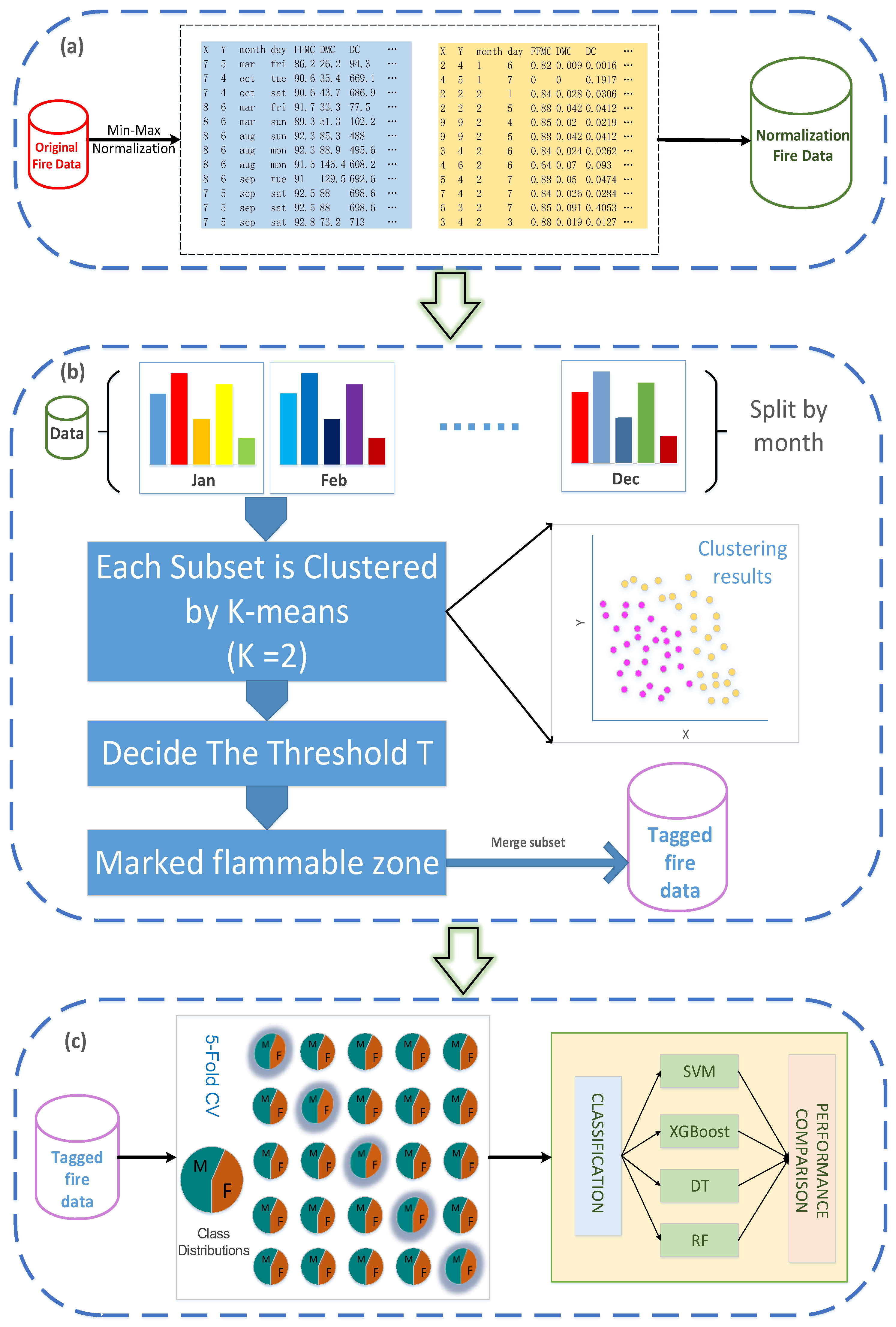
2.3. Data Preprocessing

The original dataset has a total of 13 properties, 4 of which (X, Y, month, and day) are not very useful for normalization; thus, they are removed individually, and the remaining 9 features are aggregated into new datasets (NDs). The features in the new datasets are linearly mapped using the min–max normalization technique for the transformed range of 0 to 1 because of the clustering algorithm’s sensitivity to distance. The formula for the min–max normalization method is as follows:
e n o w = e i M I N l i s t M A X l i s t M I N l i s t ( e u p e l o w ) + e l o w ,
where e i is the feature element, M A X l i s t is the highest value of the existing data in the feature, M I N l i s t is the minimum value of the existing data in the feature, and e u p and e l o w are the upper and lower bounds of the data range after linear transformation, which in this experiment is taken as (0, 1). The modifications before and after feature pre-processing are depicted in Figure 2b.

2.4. Grouping the Datasets
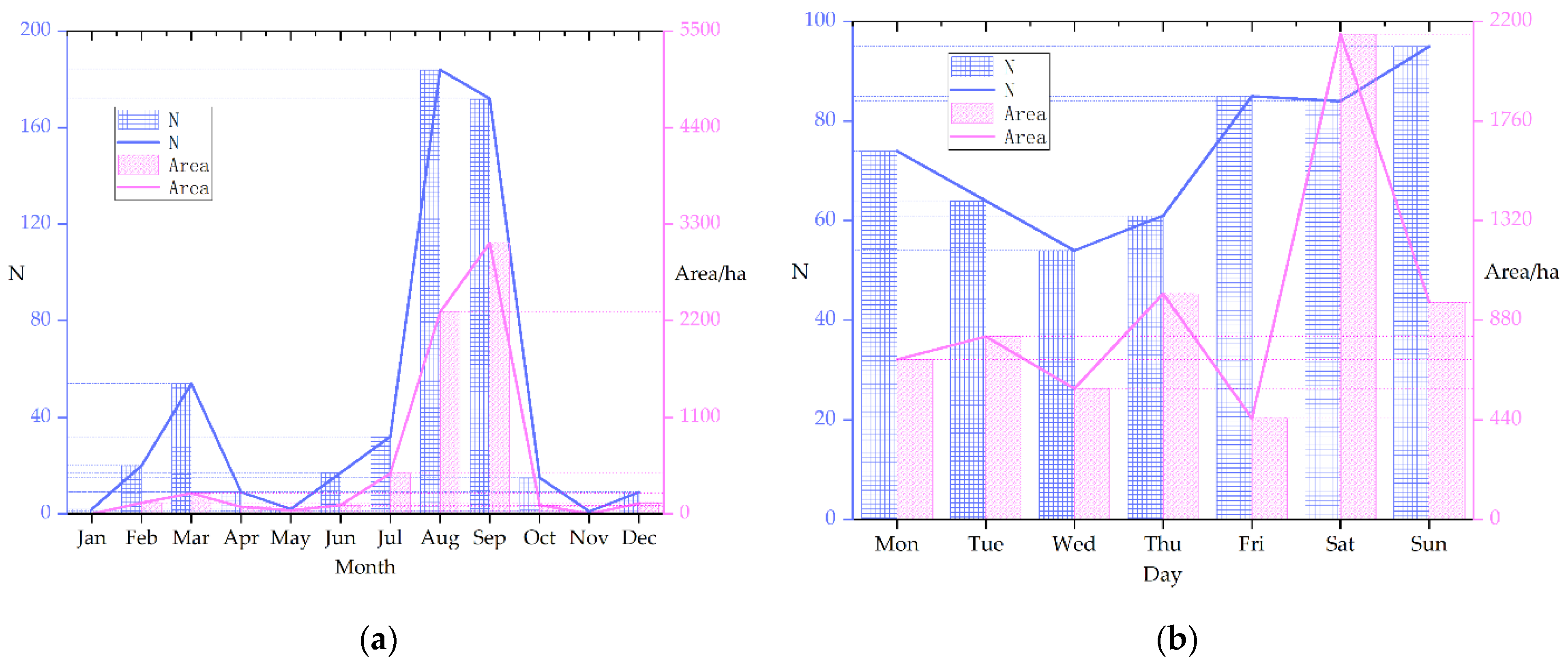
The substantial association between fires and the monthly time series may be shown by temporally periodizing the data, while the distinctive geographical patterns of the different subsets of fire activity can be seen through a deconstruction of the grid cells [36]. The following data sample split was used in this experiment to look at the link between fire incidence and spatiotemporal heterogeneity.

2.4.1. Time Series

“Month” and “day” are the properties linked with the temporal dimension in the source data. First, the normalized ND is separated into 12 subsets, depending on the month attribute of the original dataset, to identify a link between forest fire occurrence and the two temporal variables.
O r i g i n a l D a t a s e t s = { d m 1 , d m 2 , , d m 12 } | m o n t h ,
In each subgroup, the number of forest fires (n) and the total area are calculated, and the number of monthly fires and the total area are plotted, with the month as the X-axis and n and area as the Y-axis, as shown in Figure 3a.
Similarly, based on the value of the “day” variable, the data are separated into seven groups. Figure 3b shows the statistical results.
O r i g i n a l D a t a s e t s = { d d 1 , d d 2 , , d d 7 } | d a y ,
Figure 3a shows that the number of forest fires that occur each month and the total burned area are both trending in the same direction. The overall burned area and the number of fires fluctuated dramatically from month to month, demonstrating that the month has a substantial impact on forest fire production. Figure 3b shows that the total number of forest fires did not change significantly, and the trend in the total daily burned area did not correlate well with the total number of forest fires per day, indicating that the relationship between forest fire occurrence and a specific day of the week is not obvious. As a result, the month attribute was used as the foundation for splitting the time axis and discarding the predicted association between the “day” attribute and the incidence of forest fires.

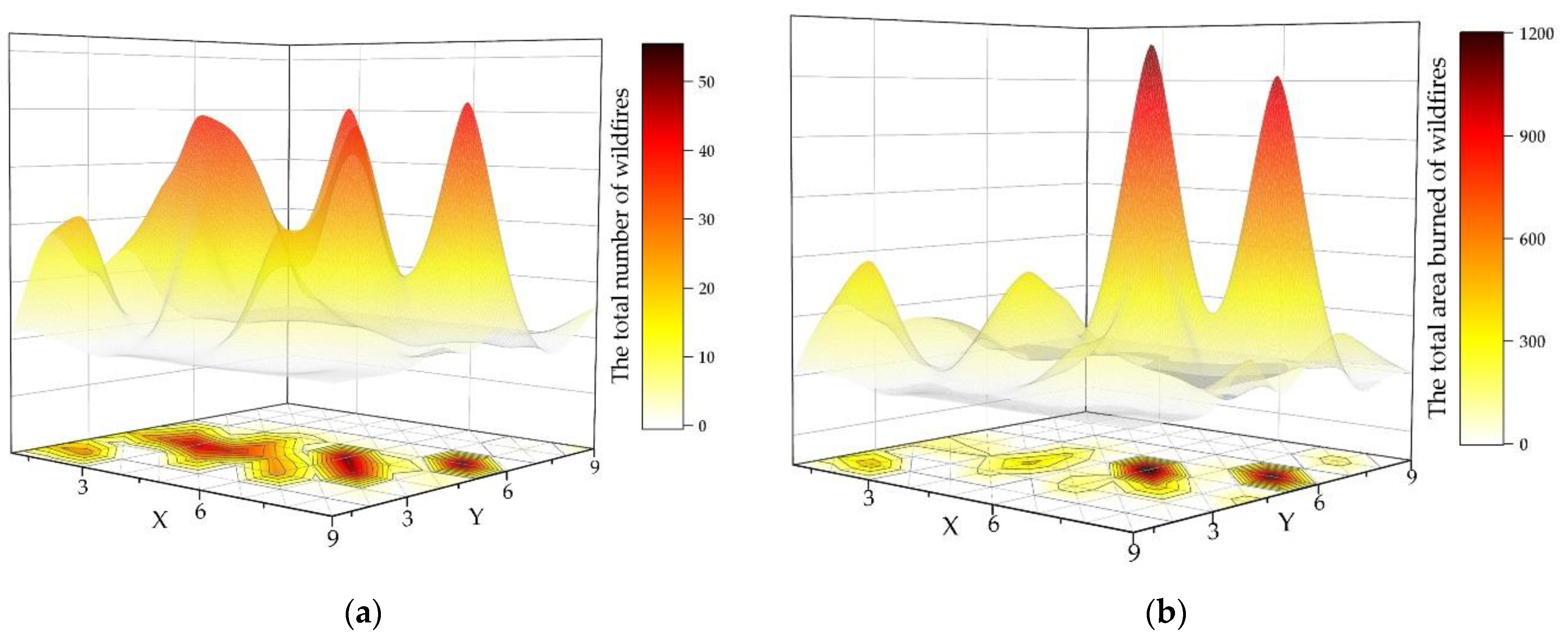
2.4.2. Spatial Series

The original dataset has two geographical location attributes: X and Y. These two characteristics define the only blocks where forest fires can occur. To look for a link between wildfires and their location, the dataset was partitioned into 81 blocks based on the original 9 × 9 grid in the data, which equates to 81 subsets, as follows:
O r i g i n a l D a t a s e t s = { d a 1 , d a 2 , , d a 81 } | b l o c k ,
In each subgroup, the total number and the area of the wildfires were calculated, and the results are set out in Figure 4. The number of wildfires and the total area within each sub-region fluctuate significantly; the trend between the number of wildfires and the total area is essentially the same, as shown in the figure. This is an excellent indicator of the relationship between forest fire incidence and geographic location.

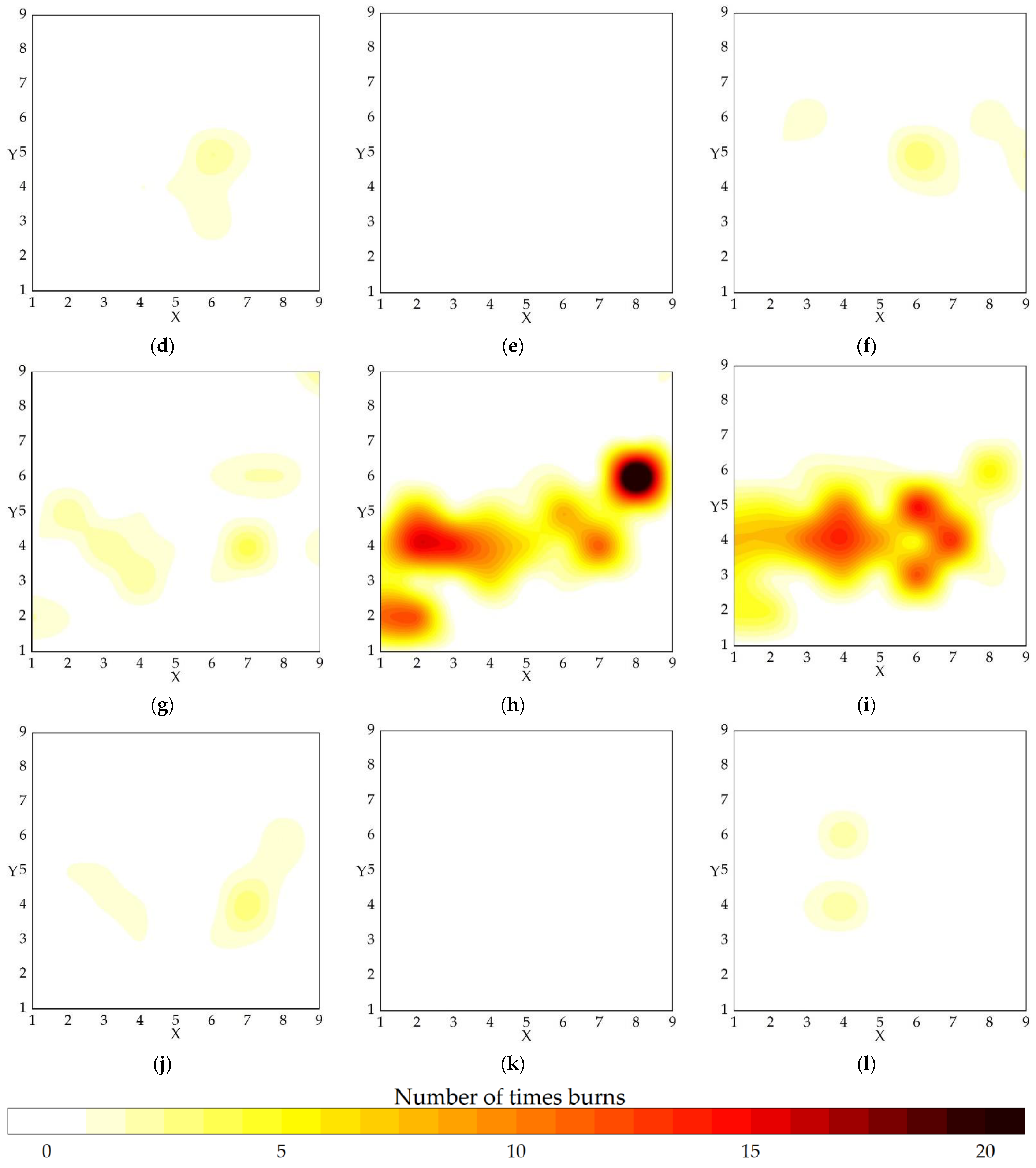
2.4.3. Time and Space Division

The preceding two sections show that the wildfire incidence is strongly linked to both temporal (month) and geographical (block) factors (X, Y). To represent this association in the data, we separated the ND into 12 subgroups based on month and then further subdivided each subset into 81 smaller sections based on the X and Y coordinates. Figure 5 and Figure 6 indicate the number and the area of wildfires for each block in each month.

2.5. K-Means Cluster

The K-means method [37] is a traditional division-based clustering technique, which is extensively utilized in large-scale data clustering due to its efficiency. Many algorithms are currently being developed and refined around this approach.
The K-means approach requires a number K , which groups the dataset into K clusters ( C 1 , C 2 , , C k | k [ 1 , K ] ). The cost function of K-means clustering is:
J = k = 0 K x C k x μ k 2 2 ,
where μ k is the mean vector of cluster C k , sometimes called the center of mass, with the expression:
μ k = 1 | C k | x C k x ,
D. Arthur et al. [38] presented the K-means++ method to overcome the problem of the sensitivity of K-means to the initialized center of mass by utilizing initialized clustering centers that are as far away as feasible.
In this experiment, to investigate the similarities between flammable and non-flammable fires, 12 subsets ( d m ) were separately clustered using the K-means++ algorithm, with the K value set to 2 (flammable fires, non-flammable fires). A link was discovered between the clustering findings and the blocks where forest fires occurred, with fire sites from the same cluster frequently being found in many blocks. In the experiment, we used the clustering findings and the distribution of fire spots inside each block to automatically create a dynamic threshold (i.e., the number of fires starting within each block), which would split the fire region into flammable and non-flammable zones in each month.

2.6. Machine Learning Models

2.6.1. XGBoost

By adding a regular term to the GBDT algorithm’s loss function to discover the best solution and increase the resistance to overfitting, the XGBoost [39] technique is meant to manage the accuracy of the GBDT [40] algorithm and avoid overfitting. Thus, the loss function of the XGBoost algorithm is:
L ( y i , y ^ i ) = i = 1 N l ( y i , y ^ i ) + m = 1 M Ω ( f m ) ,
where l ( y i , y ^ i ) is the GBDT loss function, y i denotes the actual value, y ^ i denotes the forecast value, and Ω is the canonical term and denotes the model’s complexity. The number of trees is denoted by M , while the m th tree is denoted by f m .
Ω ( f ) = γ T + 1 2 λ ω 2 ,
T is the total number of leaves in each tree, and ω is the leaf node score, while γ and ω are the user-determined parameters.

2.6.2. Support Vector Machine

The SVM is a high-performing classifier. For two labeled sets of vectors, the SVM provides an ideal partitioning surface that splits the two sets of vectors into two sides as much as is feasible and maximizes the shortest distance between the two sets of vectors to this hyperplane.

2.6.3. Decision Tree

The essence of the DT is a set of generalized classification rules from the training set. The entire DT learning process is a process of iteratively picking the best features and partitioning the dataset based on them, such that each sample is optimally classified. The DT is the foundation of common integrated learning models such as RFs and GBDTs, and it has a strong reputation in the field of machine learning.

2.6.4. Random Forest

The RF is a learning algorithm that is integrated and is based on the concept of bagging. The random forest is made up of multiple unrelated decision trees, and rather than using all of the data’s features for training, a random selection of a portion of the samples is made before constructing each decision tree. When a new sample is input after the forest has been obtained, each decision tree within the RF is voted on, and the sample is predicted to be the category with the most votes. The RF is less prone to overfitting and more noise resistant than the DT.

2.7. Performance Evaluation Metrics

After model training, three metrics—accuracy (ACC), F1 score (F1), and area under the curve (AUC) values—were used to assess the four models, and each parameter is explained as follows.
ACC: the ratio of the number of samples properly categorized by the classifier to the total number of samples is defined as accuracy, which refers to the model’s prediction accuracy. There are two sorts of samples in the number of correctly categorized samples: (1) the number of samples accurately predicted by positive classes (TP) and (2) the number of samples correctly predicted by negative classes (TN). The total number of samples is n . The formula is as follows:
A C C = T P + T N N ,
F1: precision (P) and recall (R) are weighted 1:1 to obtain the F1 index. Precision denotes the proportion of positive samples among those classified as positive cases by the classifier, whereas recall denotes the proportion of positive samples predicted by the classifier among all the positive samples. The formula is as follows:
F 1 = 2 × P × R P + R ,
AUC: the AUC (area under the curve) value is the area of the geometry below the ROC (receiver operating characteristic) curve (see Figure 7). The AUC value is usually between 0.5 and 1.0, and a higher AUC indicates that the model is more predictive.

3. Results

Five hundred and seventeen samples were labeled using ‘X’, ‘Y’, and K-means++, with 254 positive (flammable flames) and 263 negative samples (non-flammable fires). The models contained ten features: X, Y, FFMC, DMC, DC, ISI, temp, RH, wind, and rain. Because the attribute “month” was used to divide the data, it was removed here. As “day” is not a feature that is sensitive to spatial and temporal variation, it is likewise excluded here. “Area” is not a feature that existed prior to the wildfire; hence, it is likewise removed.
Four classification models were used to assess and validate the labeled data, comprising XGBoost, RF [41], SVM [42], and DT [43]. The sklearn machine learning library was used in the experiments for the auxiliary operations, and the parameters of the four models were configured as shown in Table 2. To avoid bias, the trials utilized stratified 5-fold cross validation (SFV), in which the dataset was randomly divided into five equal portions to guarantee that the percentage of the majority and minority samples in each dataset matched the original data. Four of them served as the training set, while the fifth served as the test set, with the average value produced after five times serving as the model’s overall reference result.
In this study, we employed the same model and assessment criteria as for a comparative dataset experiment using conventional markers so as to validate that spatiotemporal variables indeed have an influence on the forest fire prediction model. Traditional markers utilize the burned area (the area attribute in the dataset) to judge fire size; fires with a burned area greater than 5 ha are classified as major fires, and those with a burned area less than 5 ha are classified as minor fires [32].

Performance Evaluation Results

The AUC values of all four models are larger than 0.65 and less than 0.81, while the ACC and F1 are between 60% and 80%. These values indicate that the models result in accurate predictions. The area dashboard of the respective models for the three indicators is given in Figure 8, with K-nearest neighbor (KNN) serving as the baseline model. The greater the area, the higher the model score and the better the model effect. Figure 8 shows that the XGBoost and DT models perform better than KNN, but the RF and SVM models perform even worse. Among these, the XGBoost model has a much higher ACC and AUC, while having a nearly identical F1 to the DT model. This is due to XGBoost’s greater flexibility to small sample data and its effective ability to avoid overfitting. Table 3 shows the comprehensive evaluation findings for each model.
The data for each index were much lower than the spatiotemporal model and machine learning model findings, which employ the burned area as the foundation for fire size estimation (see Table 4). The AUC values of the old method’s prediction results are around 0.5, suggesting their model’s lack of predictive capacity.

4. Discussion

4.1. Drivers of Wildfire

A forest fire is caused by a complex interaction in terms of time, space, the status of the combustibles, the long-term weather conditions, and other factors. As can be seen from the statistics, the peak is in August and September, with over 70% of active fires happening during that time. In areas where fires have occurred, 73% of the block’s peak number of fires occurred between August and September, while the remaining blocks’ peak number of fires occurred primarily between March and July, indicating a clear monthly pattern of fires associated with spatial and temporal heterogeneity. The two nearby blocks have markedly different numbers of forest fires, despite the fact that the other elements are almost identical, which might be connected to the Montesinho Natural Park’s significant elevation fluctuations. Elevation differences cause variations in human activities and vegetation distribution fractions, impacting fire numbers, as seen in the FWI.
Weather also has a large impact on fuel availability and flammability; thus, it is a significant reason as to why wildfires occur. The regional and temporal patterns of fire weather in the Mediterranean climate are quite variable, which aids our understanding of various fire situations [44]. The four indices that have the most impact on wildfire occurrence are geographic coordinates, temporal dimension, DMC, and DC. In August, the maximum temperature and the lowest humidity of the year are found in the Montesinho Natural Park, and the plant types, as well as the high temperatures and low humidity, contribute to the spread of a significant number of wildfire sites.
Agricultural operations have decreased in the Montesinho Natural Park, but tourist and leisure activities have increased [33]. During the majority of the year, only around 200 sheep are grazed; however, from May to August, grazing activity increases dramatically. Shepherds move around 5000 sheep from lower to higher elevations to improve grazing outcomes, and shepherd activity is one of the reasons for the high incidence of wildfires at this time [45].

4.2. Limitations and Future Work

Despite the fact that this research is an improvement over the previous work, it still has several flaws. The data for the experiment were only gathered centrally during a short period of time (2000–2003), and they lacked the exact years in which the fires occurred. Due to the lack of years, it may not be possible to expand the data into longer data series per month. In this study, we demonstrated that temporal features have a significant influence on forest fire incidence, and more wildfire data products will be used in the future to better understand the dynamics and long-term development of fires throughout the year.
In this study, the studied area was the Montesinho Natural Park, which is just 742 km2 in size and covers a tiny region. Although the influence of spatial division on the forest fire prediction model was proven in this experiment, the short area span and similar geographical circumstances resulted in insignificant experimental results. To further confirm the experimental results, it is necessary to broaden the research area in order to acquire a larger and more complicated regional division. Second, because of the modifiable areal unit problem (MAUP), different scales and zoning schemes for the same study area can have an effect on the wildfire results analysis [46]. The MAUP effect could not be resolved well in this experiment due to dataset limitations.

5. Conclusions

The study of the spatiotemporal heterogeneity of wildfire occurrence is currently a prominent issue. To investigate the effect of spatiotemporal features on wildfire incidence in the Montesinho Natural Park, experiments were carried out to evaluate the fire point data using a clustering method and four classification models. The results reveal that the XGBoost-based spatiotemporal prediction model for forest fires performs better than earlier prediction models in the literature for identifying wildfires (11.37% improvement in accuracy rate). Month, geographic location, and FWI factors were determined to have the greatest impact on forest fire occurrence, followed by climate index variables. There is a non-linear relationship between forest fire drivers and the likelihood of forest fire occurrence, and there is a dynamic critical threshold between the two that is affected by changes in the month and the spatial coordinates; once this threshold is exceeded, there is a high likelihood of wildfire disasters. Predicting fire occurrence from spatial and temporal characteristics, FWI indices, and meteorological data is currently a difficult problem to solve because fire occurrence is also influenced by human activities and surface phenology [47], and the effects of climate change on fires are difficult to account for [48]. Humans are both a source of fires and a facilitator of fire suppression [49], and while human activities exacerbate the severity of fires in the Montesinho Natural Park area, the rational use of human activities, such as forest thinning [50] and artificial combustible material management [51], can reduce the occurrence of fires. For the investigation of the geographical and temporal aspects of fires in the future, a larger experimental region and a longer time axis should be considered. The analysis of parameters such as population density and vegetation distribution can also improve the performance of spatiotemporal wildfire prediction models, allowing managers to deploy resources more rationally and to lower the danger of extensive fires.

Author Contributions

Conceptualization, Y.D.; data curation, H.W. and H.D.; formal analysis, P.S.; funding acquisition, P.S.; investigation, H.D.; methodology, H.D. and H.W; resources, P.S.; supervision, Y.D.; writing—original draft, H.D.; writing—review and editing, H.D. and Y.D. All authors have read and agreed to the published version of the manuscript.

Funding

This research received no external funding.

Institutional Review Board Statement

Not applicable.

Informed Consent Statement

Not applicable.

Data Availability Statement

The dataset used in this study is available for download at https://archive.ics.uci.edu/ml/datasets/forest+fires/ (accessed on 6 May 2021).

Acknowledgments

We would like to acknowledge Cortez and Morais for collecting the forest fire dataset in Montesinho Natural Park and MDPI Magazine for its linguistic assistance during the preparation of this manuscript.

Conflicts of Interest

The authors declare no conflict of interest.

References

  1. Santos, S.; Bento-Gonçalves, A.; Vieira, A. Research on Wildfires and Remote Sensing in the Last Three Decades: A Bibliometric Analysis. Forests 2021, 12, 604. [Google Scholar] [CrossRef]
  2. Ribeiro-Kumara, C.; Köster, E.; Aaltonen, H.; Köster, K. How do forest fires affect soil greenhouse gas emissions in upland boreal forests? A review. Environ. Res. 2020, 184, 109328. [Google Scholar] [CrossRef]
  3. Seidl, R.; Thom, D.; Kautz, M.; Martin-Benito, D.; Peltoniemi, M.; Vacchiano, G.; Wild, J.; Ascoli, D.; Petr, M.; Honkaniemi, J.; et al. Forest disturbances under climate change. Nat. Clim. Chang. 2017, 7, 395–402. [Google Scholar] [CrossRef] [PubMed]
  4. Shukla, P.R.; Skea, J.; Buendia, E.C.; Masson-Delmotte, V.; Portner, H.-O.; Roberts, D.C.; Zhai, P.; Slade, R.; Connors, S.; van Diemen, R.; et al. (Eds.) Change and Land: An IPCC Special Report on Climate Change, Desertification, Land Degradation, Sustainable Land Management, Food Security, and Greenhouse Gas Fluxes in Terrestrial Ecosystems; in press.
  5. Halofsky, J.E.; Peterson, D.L.; Harvey, B.J. Changing wildfire, changing forests: The effects of climate change on fire regimes and vegetation in the Pacific Northwest, USA. Fire Ecol. 2020, 16, 4. [Google Scholar] [CrossRef]
  6. Huffman, D.W.; Roccaforte, J.P.; Springer, J.D.; Crouse, J.E. Restoration applications of resource objective wildfires in western US forests: A status of knowledge review. Fire Ecol. 2020, 16, 1–13. [Google Scholar] [CrossRef]
  7. Sirin, A.; Medvedeva, M. Remote Sensing Mapping of Peat-Fire-Burnt Areas: Identification among Other Wildfires. Remote Sens. 2022, 14, 194. [Google Scholar] [CrossRef]
  8. Ma, W.; Feng, Z.; Cheng, Z.; Chen, S.; Wang, F. Identifying Forest Fire Driving Factors and Related Impacts in China Using Random Forest Algorithm. Forests 2020, 11, 507. [Google Scholar] [CrossRef]
  9. Abram, N.J.; Henley, B.J.; Gupta, A.S.; Lippmann, T.J.R.; Clarke, H.; Dowdy, A.J.; Sharples, J.J.; Nolan, R.H.; Zhang, T.; Wooster, M.J.; et al. Connections of climate change and variability to large and extreme forest fires in southeast Australia. Commun. Earth Environ. 2021, 2, 1–17. [Google Scholar] [CrossRef]
  10. Sulova, A.; Arsanjani, J.J. Exploratory Analysis of Driving Force of Wildfires in Australia: An Application of Machine Learning within Google Earth Engine. Remote. Sens. 2021, 13, 10. [Google Scholar] [CrossRef]
  11. Fernandez-Anez, N.; Krasovskiy, A.; Müller, M.; Vacik, H.; Baetens, J.; Hukić, E.; Solomun, M.K.; Atanassova, I.; Glushkova, M.; Bogunović, I.; et al. Current Wildland Fire Patterns and Challenges in Europe: A Synthesis of National Perspectives. Air, Soil Water Res. 2021, 14, 11786221211028185. [Google Scholar] [CrossRef]
  12. Febriandhika, A.I.; Rahman, C.T.; Ramdani, F.; Saputra, M.C.; IEEE. Tangible Landscape: Simulation of Estimation of Wildfire Spread in Arjuno Mountain Tahura R. Soerjo Region. In Proceedings of the 4th International Symposium on Geoinformatics (ISyG), Malang, Indonesia, 10–12 November 2018. [Google Scholar]
  13. Jain, P.; Coogan, S.C.P.; Subramanian, S.G.; Crowley, M.; Taylor, S.W.; Flannigan, M.D. A review of machine learning applications in wildfire science and management. Environ. Rev. 2020, 28, 478–505. [Google Scholar] [CrossRef]
  14. Jaafari, A.; Zenner, E.K.; Pham, B.T. Wildfire spatial pattern analysis in the Zagros Mountains, Iran: A comparative study of decision tree based classifiers. Ecol. Inform. 2018, 43, 200–211. [Google Scholar] [CrossRef]
  15. Gigović, L.; Pourghasemi, H.R.; Drobnjak, S.; Bai, S. Testing a New Ensemble Model Based on SVM and Random Forest in Forest Fire Susceptibility Assessment and Its Mapping in Serbia’s Tara National Park. Forests 2019, 10, 408. [Google Scholar] [CrossRef]
  16. Collins, L.; McCarthy, G.; Mellor, A.; Newell, G.; Smith, L. Training data requirements for fire severity mapping using Landsat imagery and random forest. Remote Sens. Environ. 2020, 245, 111839. [Google Scholar] [CrossRef]
  17. Michael, Y.; Helman, D.; Glickman, O.; Gabay, D.; Brenner, S.; Lensky, I.M. Forecasting fire risk with machine learning and dynamic information derived from satellite vegetation index time-series. Sci. Total Environ. 2020, 764, 142844. [Google Scholar] [CrossRef]
  18. Hantson, S.; Arneth, A.; Harrison, S.P.; Kelley, D.I.; Prentice, I.C.; Rabin, S.S.; Archibald, S.; Mouillot, F.; Arnold, S.R.; Artaxo, P.; et al. The status and challenge of global fire modelling. Biogeosciences 2016, 13, 3359–3375. [Google Scholar] [CrossRef]
  19. Saha, M.V.; Scanlon, T.M.; D’Odorico, P. Climate seasonality as an essential predictor of global fire activity. Glob. Ecol. Biogeogr. 2018, 28, 198–210. [Google Scholar] [CrossRef]
  20. Spitz, D.B.; Clark, D.A.; Wisdom, M.J.; Rowland, M.M.; Johnson, B.K.; Long, R.A.; Levi, T. Fire history influences large-herbivore behavior at circadian, seasonal, and successional scales. Ecol. Appl. 2018, 28, 2082–2091. [Google Scholar] [CrossRef] [PubMed]
  21. Abouali, A.; Raposo, J.R.; Viegas, D.X. The role of the terrain-modified wind on driving the fire behaviour over hills-an Experimental and Numerical Analysis. In Proceedings of the 8th International Conference on Forest Fire Research, Coimbra, Portugal, 9–16 November 2018; pp. 677–694. [Google Scholar] [CrossRef]
  22. LeVine, D.; Crews, K. Time series harmonic regression analysis reveals seasonal vegetation productivity trends in semi-arid savannas. Int. J. Appl. Earth Obs. Geoinf. ITC J. 2019, 80, 94–101. [Google Scholar] [CrossRef]
  23. Silveira, E.M.D.O.; Espírito-Santo, F.D.B.; Acerbi-Júnior, F.W.; Galvão, L.S.; Withey, K.D.; Blackburn, G.A.; De Mello, J.M.; Shimabukuro, Y.E.; Domingues, T.; Scolforo, J.R.S. Reducing the effects of vegetation phenology on change detection in tropical seasonal biomes. GIScience Remote Sens. 2018, 56, 699–717. [Google Scholar] [CrossRef]
  24. Freitas, W.; Gois, G.; Pereira, E.; Junior, J.O.; Magalhães, L.; Brasil, F.; Sobral, B. Influence of fire foci on forest cover in the Atlantic Forest in Rio de Janeiro, Brazil. Ecol. Indic. 2020, 115, 106340. [Google Scholar] [CrossRef]
  25. Rakhmatulina, E.; Stephens, S.; Thompson, S. Soil moisture influences on Sierra Nevada dead fuel moisture content and fire risks. For. Ecol. Manag. 2021, 496, 119379. [Google Scholar] [CrossRef]
  26. Varela, V.; Vlachogiannis, D.; Sfetsos, A.; Karozis, S.; Politi, N.; Giroud, F. Projection of Forest Fire Danger due to Climate Change in the French Mediterranean Region. Sustainability 2019, 11, 4284. [Google Scholar] [CrossRef]
  27. Jang, E.; Kang, Y.; Im, J.; Lee, D.-W.; Yoon, J.; Kim, S.-K. Detection and Monitoring of Forest Fires Using Himawari-8 Geostationary Satellite Data in South Korea. Remote Sens. 2019, 11, 271. [Google Scholar] [CrossRef]
  28. Chen, Y.; Randerson, J.T.; Coffield, S.R.; Foufoula-Georgiou, E.; Smyth, P.; Graff, C.A.; Morton, D.C.; Andela, N.; van der Werf, G.R.; Giglio, L.; et al. Forecasting Global Fire Emissions on Subseasonal to Seasonal (S2S) Time Scales. J. Adv. Model. Earth Syst. 2020, 12, e2019MS001955. [Google Scholar] [CrossRef] [PubMed]
  29. Liu, J.; Wang, D.; Maeda, E.E.; Pellikka, P.K.E.; Heiskanen, J. Mapping Cropland Burned Area in Northeastern China by Integrating Landsat Time Series and Multi-Harmonic Model. Remote Sens. 2021, 13, 5131. [Google Scholar] [CrossRef]
  30. Zhou, Q.; Rover, J.; Brown, J.; Worstell, B.; Howard, D.; Wu, Z.; Gallant, A.L.; Rundquist, B.; Burke, M. Monitoring Landscape Dynamics in Central U.S. Grasslands with Harmonized Landsat-8 and Sentinel-2 Time Series Data. Remote Sens. 2019, 11, 328. [Google Scholar] [CrossRef]
  31. Carvalho, N.S.; Anderson, L.O.; Nunes, C.A.; Pessôa, A.C.M.; Junior, C.H.L.S.; dos Reis, J.B.C.; Shimabukuro, Y.E.; Berenguer, E.; Barlow, J.; Aragao, L.E. Spatio-temporal variation in dry season determines the Amazonian fire calendar. Environ. Res. Lett. 2021, 16, 125009. [Google Scholar] [CrossRef]
  32. Xie, Y.; Peng, M. Forest fire forecasting using ensemble learning approaches. Neural Comput. Appl. 2018, 31, 4541–4550. [Google Scholar] [CrossRef]
  33. Evelpidou, N.; de Figueiredo, T.; Mauro, F.; Tecim, V.; Vassilopoulos, A. Natural Heritage from East to West: Case Studies from 6 EU Countries; Springer: Berlin/Heidelberg, Germany, 2010; pp. 119–132. [Google Scholar]
  34. Neves, J.M.; Santos, M.F.; Machado, J.M. (Eds.) New trends in artificial intelligence. In Proceedings of the 13th Portuguese Conference on Artificial Intelligence (EPIA 2007), Guimarães, Portugal, 3–7 December 2007; APPIA: Lisaboa, Portugal, 2007; pp. 512–523, ISBN 978-989-95618-0-9. [Google Scholar]
  35. Van Wagner, C.E. Development and Structure of the Canadian Forest Fire Weather Index System; Forestry Technical Report 35; Canadian Forestry Service, Headquarters: Ottawa, ON, Canada, 1987; 35p. [Google Scholar]
  36. Jiménez-Ruano, A.; Mimbrero, M.R.; Jolly, W.M.; Fernández, J.D.L.R. The role of short-term weather conditions in temporal dynamics of fire regime features in mainland Spain. J. Environ. Manag. 2018, 241, 575–586. [Google Scholar] [CrossRef]
  37. MacQueen, J. Some methods for classification and analysis of multivariate observations. In Proceedings of the Fifth Berkeley Symposium on Mathematical Statistics and Probability; University of California Press: Berkeley, CA, USA, 1967; Volume 1, pp. 281–297. [Google Scholar]
  38. Arthur, D.; Vassilvitskii, S. k-means plus plus: The Advantages of Careful Seeding. In Proceedings of the 18th ACM-SIAM Symposium on Discrete Algorithms, New Orleans, LA, USA, 7–9 January 2007. [Google Scholar]
  39. Chen, T.; Guestrin, C. XGBoost: A Scalable Tree Boosting System. In Proceedings of the 22nd ACM SIGKDD International Conference on Knowledge Discovery and Data Mining (KDD), San Francisco, CA, USA, 13–17 August 2016; pp. 785–794. [Google Scholar] [CrossRef]
  40. Friedman, J.H. Greedy function approximation: A gradient boosting machine. Ann. Stat. 2001, 29, 1189–1232. [Google Scholar] [CrossRef]
  41. Breiman, L. Random forests. Mach. Learn. 2001, 45, 5–32. [Google Scholar] [CrossRef]
  42. Vapnik, V.N. The Nature of Statistical Learning Theory, 2nd ed.; Springer: New York, NY, USA, 2000; p. 314. [Google Scholar]
  43. Salzberg, S.L. Book Review: C4.5: Programs for Machine Learning by J. Ross Quinlan. Morgan Kaufmann Publishers, Inc., 1993. Mach. Learn. 1994, 16, 235–240. [Google Scholar] [CrossRef]
  44. Calheiros, T.; Nunes, J.P.; Pereira, M. Recent evolution of spatial and temporal patterns of burnt areas and fire weather risk in the Iberian Peninsula. Agric. For. Meteorol. 2020, 287, 107923. [Google Scholar] [CrossRef]
  45. Geraldes, A.; Boavida, M. Distinct age and landscape influence on two reservoirs under the same climate. Hydrobiologia 2003, 504, 277–288. [Google Scholar] [CrossRef]
  46. Nagle-McNaughton, T.; Gong, X.; Constantine, J.A. Implications of the modifiable areal unit problem for wildfire analyses. Adv. Biol. Earth Sci. 2019, 4, 150–175. [Google Scholar]
  47. Wang, J.; Zhang, X.; Rodman, K. Land cover composition, climate, and topography drive land surface phenology in a recently burned landscape: An application of machine learning in phenological modeling. Agric. For. Meteorol. 2021, 304–305, 108432. [Google Scholar] [CrossRef]
  48. Parente, J.; Pereira, M.G.; Tonini, M. Space-time clustering analysis of wildfires: The influence of dataset characteristics, fire prevention policy decisions, weather and climate. Sci. Total Environ. 2016, 559, 151–165. [Google Scholar] [CrossRef]
  49. Fernandes, P.M. Variation in the Canadian Fire Weather Index Thresholds for Increasingly Larger Fires in Portugal. Forests 2019, 10, 838. [Google Scholar] [CrossRef]
  50. Banerjee, T. Impacts of Forest Thinning on Wildland Fire Behavior. Forests 2020, 11, 918. [Google Scholar] [CrossRef]
  51. Benali, A.; Sá, A.; Pinho, J.; Fernandes, P.; Pereira, J. Understanding the Impact of Different Landscape-Level Fuel Management Strategies on Wildfire Hazard in Central Portugal. Forests 2021, 12, 522. [Google Scholar] [CrossRef]
Figure 1. Terrain distribution map of Montesinho Natural Park, Portugal.
Sustainability 14 10107 g001
Figure 2. The three key steps of the experiment are as follows: (a) pre-process the data using the min–max normalization technique, due to the sensitivity of the K-means++ clustering methodology to distance fluctuation; (b) investigate the link between climate changes and time; the overall sample is divided into numerous sub-samples along the time axis; discover the relationship between sample distribution and the presence of spatial dimensions and use spatial coordinates to grid the forest fire data; generalize the common features within each sub-dataset, compare the clustering results to the geographical division findings, and label the dataset with the clustering technique; (c) for wildfire-prone region prediction, the labeled subsets were concatenated as the complete sample set with labeling, and four machine learning methods were applied. Figure 2 depicts the model’s architecture.
Sustainability 14 10107 g002
Figure 3. Total number of wildfires and total areas burned (in hectares): (a) total number of wildfires and total areas burned per month; (b) number of wildfires and total areas burned on each day of the week. The figure shows that the number and area of wildfires vary greatly with “month”, but relatively little with “day”, which is why “month” was chosen as the time division in the experiment.
Sustainability 14 10107 g003
Figure 4. Total number of wildfires and total areas burned in each block (in hectares): (a) distribution of the number of wildfires; (b) distribution of the total areas burned.
Sustainability 14 10107 g004
Figure 5. Number of times burned by wildfires (NB) in the 81 blocks during each month: (al) for January–December, respectively. The figure shows that the NB varies greatly from month to month and is unevenly distributed within each block, a phenomenon that provides a basis for the spatial and temporal delineation of wildfires.
Sustainability 14 10107 g005aSustainability 14 10107 g005b
Figure 6. The distribution of burned areas (NA) in the 81 blocks in each month: (al) for January–December, respectively. The figure shows that the NA varies greatly from month to month and the regional distribution of the center of gravity is different, a phenomenon that provides a basis for the spatial and temporal division of wildfires.
Sustainability 14 10107 g006aSustainability 14 10107 g006b
Figure 7. Geometric interpretation of the values for area under the curve (AUC) of receiver operating characteristics (ROCs); the shaded area is the AUC value.
Sustainability 14 10107 g007
Figure 8. The evaluation results of spatiotemporal models on the test set. Using the score of the K−nearest neighbor (KNN) model as the benchmark (the dashed part in the figure is the KNN model score), a line graph of the area of the four machine learning model scores is drawn, and the larger the area, the better the model effect. The four models are extreme gradient boosting (XGBoost), random forest (RF), support vector machine (SVM), and decision tree (DT). The evaluation indexes of the model are accuracy (ACC), F1 Score (F1), and the values for the area under the curve (AUC) of the receiver operating characteristics.
Sustainability 14 10107 g008
Table 1. Variables in the wildfire dataset described in great detail.
AbbreviationVariablesExplanations
Location XX-axis spatial coordinates (1 ≤ X ≤ 9)
YY-axis spatial coordinates (1 ≤ Y ≤ 9)
Time series MonthMonths of the year (from January to December)
DayDays of the week (from Monday to Sunday)
FWIFFMCfine fuel moisture codeWater content of cured fine fuels (from 18.7 to 96.20), with a time period of 16 h
DMCduff moisture codeWater content of surface combustible material (from 1.1 to 291.3) in the upper layer of forest humus, with a time period of 12 days
DCdrought codeIndex of the effect of prolonged drought on forest combustibles (7.9–860.6), with a time period of 52 days
ISIinitial spread indexThe initial rate of fire spread (from 0 to 56.10)
Climatic conditionstemptemperature Temperature (Celsius) (from 2.2 to 33.30)
RHrelative humidityRelative humidity (%) (from 15.0 to 100)
WindWind speed (km/h) (from 0.40 to 9.40)
RainOutdoor rainfall (mm/m2) (from 0.0 to 6.40)
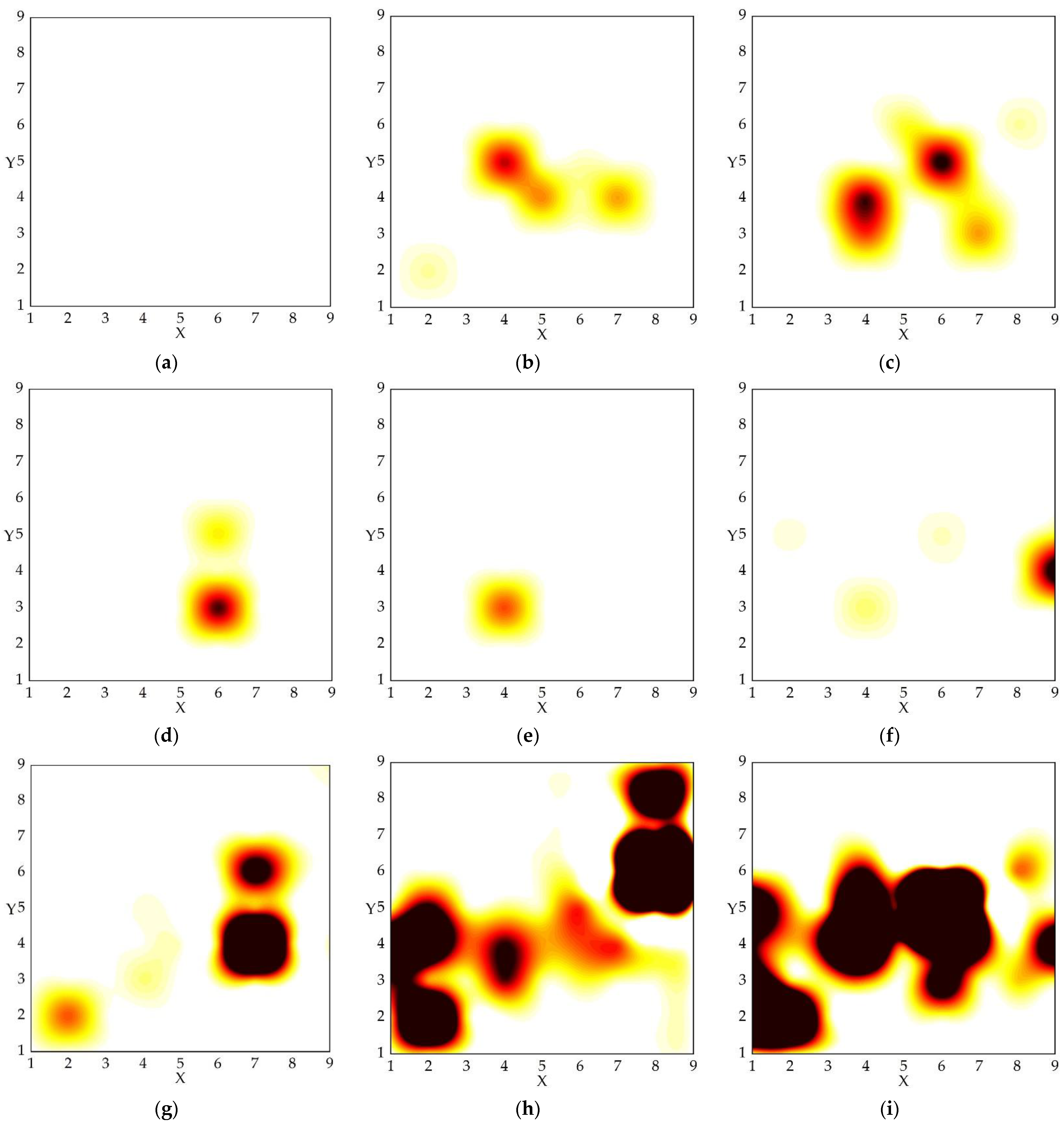
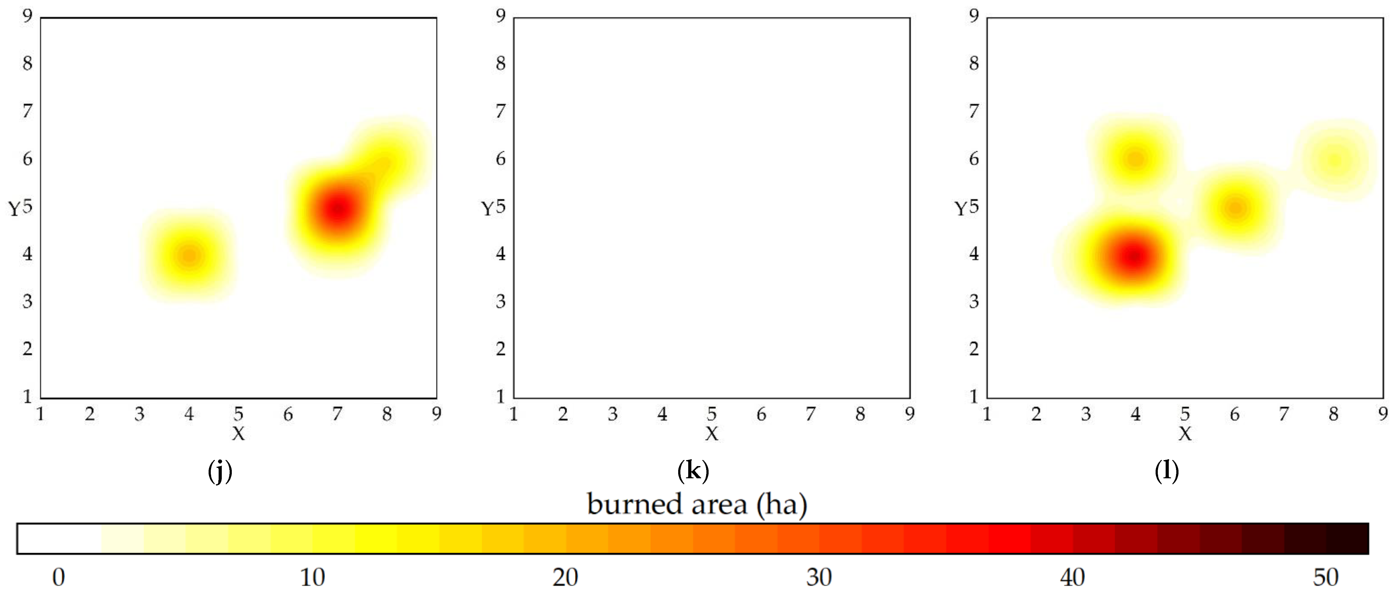
Burned area AreaTotal forest burned area (ha) (0.00~1090.84)
Table 2. Parameter settings for the four models. The four models are extreme gradient boosting (XGBoost), random forest (RF), support vector machine (SVM), and decision tree (DT).
ModelParameters
XGBoostmax_depth = 3; min_child_weight = 1; gamma = 0.1
colsample_bytree = 1; scale_pos_weight = 1; learing_rate = 0.05
n_estimators = 500; silent = 1; colsample_bytree = 1
early_stopping_rounds = 100; eval_metric = “logloss”
RFmax_depth = 5; n_estimators = 10; max_fearure = 1
n_estimators = 500; min_samples_split = 2
SVMKernel = ‘linear’; degree = 3; tol = 0.001
DTcriterion = “gini”; min_samples_split = 2; min_samples_leaf = 1
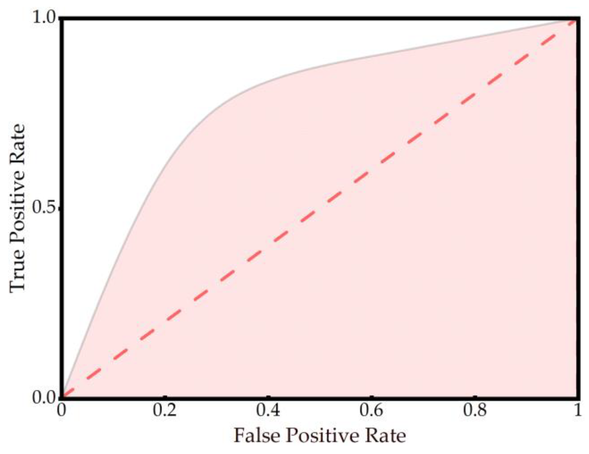
Table 3. Evaluation results of the four machine learning models based on spatiotemporal characteristics.
ModelAccuracy (ACC)F1 Score (F1)AUC 1
XGBoost0.81320.78620.8052
RF0.72040.71220.7204
SVM0.67220.63220.6724
DT0.79680.78800.7966
1 AUC is the value for area under the curve of receiver operating characteristics (ROC).
Table 4. Evaluation results of the four machine learning models based on the approach of classifying wildfires by burned area size.
ModelACCF1AUC
XGBoost0.63660.44840.4804
RF0.68460.42580.4912
SVM0.70820.41460.5000
DT0.53220.46000.4648
Publisher’s Note: MDPI stays neutral with regard to jurisdictional claims in published maps and institutional affiliations.

