Article

Application of Machine Learning (ML) and Artificial Intelligence (AI)-Based Tools for Modelling and Enhancing Sustainable Optimization of the Classical/Photo-Fenton Processes for the Landfill Leachate Treatment

1
Department of Geomatic Engineering, Giresun University, Giresun 28200, Türkiye
2
Department of Environmental Engineering, Institute of Science, Nevşehir Hacı Bektaş Veli University, Nevşehir 50300, Türkiye
*
Author to whom correspondence should be addressed.
Sustainability 2022, 14(18), 11261; https://0-doi-org.brum.beds.ac.uk/10.3390/su141811261
Submission received: 20 July 2022 / Revised: 26 August 2022 / Accepted: 4 September 2022 / Published: 8 September 2022

Abstract

:
This study presents a machine learning (ML)/artificial intelligence (AI)-based perspective to reliably predict and enhance the treatment efficiency of landfill leachate by classical-Fenton (c-Fenton) and photo-Fenton (p-Fenton) processes. This experiment also sought to lower treatment costs by evaluating the impact of using different numbers of UV-c (254 nm) lamps during p-Fenton processes, as well as to develop a sustainable process design for landfill leachate. In the modeling stage, the radial basis function neural network (RBFN), the feed forward neural network (FFNN), and the support vector regression (SVR) were used and the results were evaluated in a broad scanning. Our experimental results, optimized with the help of genetic algorithm (GA), showed an increasing trend in treatment efficiency and a decreasing trend in chemical usage amounts for p-Fenton oxidation. The results indicate that both treatment techniques performed (classical and p-Fenton) within 1 h contact time showed a very high pollutant removal with a reduction in COD of approximately 60% and 80%, respectively, during the first 30 min of processing. Additionally, it was noted that the COD elimination for the c-Fenton and the p-Fenton was significantly finished in first 15 min, 52% and 73%, respectively. According to the results of the optimization model, there is an increase from 62 to 82 percent under eight UV lamps compared to seven UV lamps when considering the impact of the number of UV lamps on the treatment efficiency in p-Fenton. It has been noted that when the results are taken as a whole, the better modeling abilities of ML-based models, particularly the RBFN and the FFNN, come to the fore. From a different angle, the FFNN and the RBFNN have both shown percentile errors that are extremely close to zero when MAPE values, a percentile error measure independent of the unit of the data set, are evaluated alone. Except for two tests whose desirability levels are still around 99.99%, all experiments attained outstanding desirability levels of 100.00%. This serves as more evidence for the higher modeling performance of these ML-based approaches.

1. Introduction

In developing countries, only a small percentage of municipal solid waste is disposed of safely, while the majority remains in the streets or disposed of in open landfills [1]. Although modern landfills are highly engineered facilities designed to eliminate or minimize the adverse impact of wastes, the generation of leachates is still a major problem for sustainable solid waste management. Landfill leachate poses threats to the local ecosystems and has a detrimental effect on the survival of marine life. Due of its volume, composition and the percolation of the rainfall through the site, landfill leachate is known as the high-strength wastewater for receiving environments. In developing countries, only a small percentage of municipal solid waste is disposed of safely, while the majority remains in the streets or is disposed of in open landfills. The characteristics of leachate are widely different, mainly depending on its age, the origin of waste, and climate conditions [2,3,4,5]. Landfill leachate is typically characterized by complex organics, inorganics, xenobiotic organic compounds, heavy metals, ammonium, fulvic/humic acids, especially aromatic hydrocarbons, chlorinated aliphatics, dark color, microorganisms, and other harmful substances. In addition to their complicated chemical makeup, leachates are highly polluting and challenging to remediate since the environment and style of operation of the landfill site affect how they behave [6,7,8].
Because of the toxicity, low biodegradability, and large quantities of organic materials in older leachates, biological treatment is ineffective for removing its contaminants. This demonstrates the value of advanced oxidation processes (AOPs) as a cutting-edge technology for the elimination of hard-to-degrade chemicals, and these systems consist of different oxidation processes such as Fenton’s oxidation, photo-oxidation, and electro-oxidation, which have been widely applied. In order to increase the removal efficiency of pollutants containing especially high COD and TOC, it may be necessary to perform pretreatment (e.g., coagulation) before direct application of AOPs such as Fenton oxidation to wastewater [5,9].
The photo-Fenton process (p-Fenton) is one of the AOPs, in which acidic conditions, ferrous ions, ultraviolet light (UV) irradiation, and hydrogen peroxide decompose to produce hydroxyl radicals (OH˚). The procedure is frequently chosen because of its simple design, ability to research at different temperatures, and its vast superiority over traditional treatments [8,10,11]. One of the primary drawbacks of this AOP is that it is not thought to be an economically viable method because of the higher operating costs linked to electricity consumption. The usage of UV lamps also poses long-term health concerns, regardless of safety [12,13]. The technique is able to decompose the substantial organic load present in the landfill leachate, hence lowering the wastewater’s toxicity [10,14].
The artificial neural network (ANN) application areas considered in the survey include computer security, medical science, business, the stock market, electricity generation, nuclear industry, mining, crops yield prediction, environmental studies (water/wastewater treatment) and policy. The ability of an ANN to learn and generalize the behaviour of any complex and non-linear process makes it a powerful modeling tool [15,16]. In the literature, there are few studies in which different learning techniques are applied for the sustainable optimization of pollutant removal from various wastewater using Fenton-based processes [11,17,18,19,20,21,22,23,24,25,26]. For ANN generated from small-scale datasets, the introduction of ML/AI-based modeling is crucial for enhancing prediction accuracy.
This study presents a machine learning (ML)/artificial intelligence (AI)-based point of view to model the treatment of landfill leachate performed by classical-Fenton (c-Fenton) and photo-Fenton (p-Fenton) processes. Advanced regression models, in the framework of machine learning (ML), offer an opportunity to refine current practices [27]. This ML-based point of view involves the support vector regression (SVR), the feed forward neural network (FFNN) and the radial basis function neural network (RBFNN). These tools are widely used for regression problems in many scientific fields. One of the biggest advantages of ML prediction tools is that they can efficiently and accurately model, thanks to their ability to learn from data. These features allow them to predict parameters reliably for new experiments that are difficult or impossible to set up in terms of time and cost. This is valuable for an experimental design problem such as the treatment of the wastewater.
The performance of the ML-based modelling tools was evaluated together with the outcomes produced by Response Surface Methodology (RSM), which is a traditional statistical modeling approach. When the content of the study is considered as a whole, it includes the following operations:
  • Modelling and prediction of the sustainable treatment of landfill leachate performed by c-Fenton and p-Fenton processes via SVR, FFNN, and RBFNN.
  • Comparison of the ML-based produced results with the RSM’s outcomes by the different paths; the use of some statistical error metrics, the discussion of some features of simple linear regression analysis, and the creating and interpreting of some visual graphs.
  • Investigation of the effects of the oxidation pH, Fe2+ and H2O2 dose, and contact time on both Fenton processes,
  • Computational optimizing of the parameters of the treatment of landfill leachate realized by c-Fenton and p-Fenton processes via Genetic Algorithm (GA),
  • Evaluation and discussion of the findings as a whole.

2. Materials and Methods

In this study, a series of laboratory studies were carried out to compare the COD removal efficiencies of c-Fenton and p-Fenton processes from real solid waste landfill leachate and to model the obtained data with neural networks. In order to achieve these objectives and determine the ideal conditions for the sustainable process design in a batch reactor, the effects of pH, Fe2+ dose, H2O2 dose, H2O2/Fe2+ ratio, and contact time were examined.

2.1. Leachate

Leachate samples were taken from a landfill located in Sivas, Türkiye. The wastewater was collected into 5 L PE bottles as a 2 h composite sample, transported to the laboratory at 4 °C of storage boxes, and stored in the refrigerator for experiments. The specific characteristics of landfill leachate are listed in Table 1.

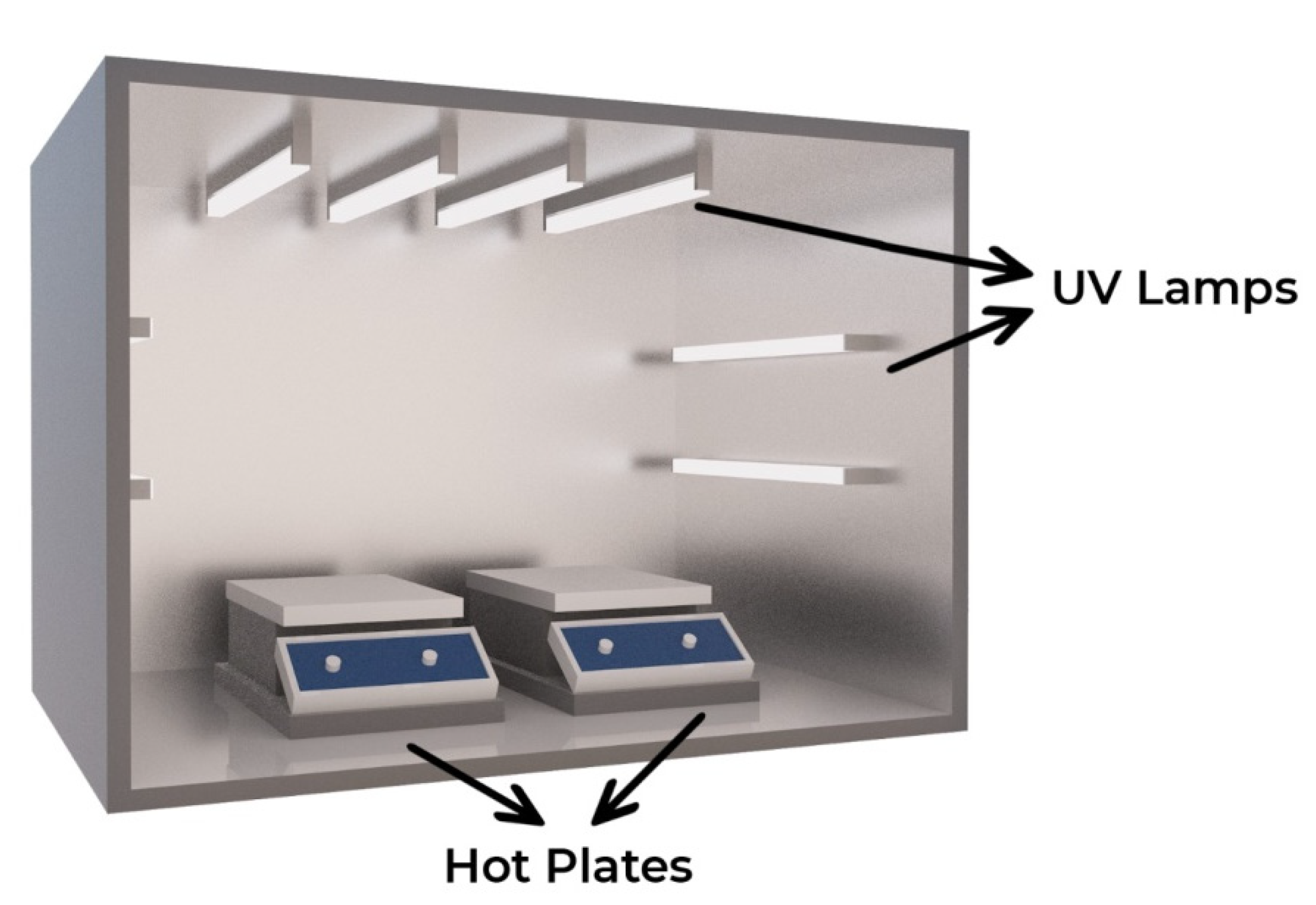
2.2. The Experiment Procedures of the Fenton Processes

The c-Fenton experiments were performed with a jar test flocculator (Velp JLT6). The p-Fenton experiments were conducted in a wooden cabinet with an aluminum exterior. Inside the process cabinet, there are eight independently controllable 8 W UV-c radiation lamps that emit light with a wavelength of 254 nm. The dimensions (L × W × H) of the cabin were 50 cm × 50 cm × 42 cm (Figure 1). The pH value of wastewater was adjusted by 3 N NaOH and 6 N H2SO4. 200 mL of pH-adjusted wastewater at 4671 mg L−1 of initial COD concentration was transferred to 500 mL of the beaker and the desired concentrations of Fe2+ and H2O2 were added to it. After the adding of reagents, fast mixing (300 rpm) and slow mixing (90 rpm) were applied to the mixture during 60 min of contact time. The pH value of the mixture was made alkaline to stop the oxidation and start the flocculation. At the end of the settling process, the supernatant phase was separated by a 0.45 µm membrane filter for COD analysis by the Closed Reflux Method. A thermoreactor (Hach LT200) was used to pre-condition the COD analysis, and COD concentration was measured by a spectrophotometer (Hach DR3900). The effects of pH, Fe2+ dose, H2O2 dose, H2O2/Fe2+ ratio, and contact time on COD removal were investigated for 1 h at a temperature of 23 ± 2 °C.

2.3. Machine Learning-Based Modelling Methods

Machine Learning (ML), in a general manner, can be defined as an automated learning process in which data patterns are processed [28]. ML can also be counted as a branch of artificial intelligence (AI) that enables systems to learn and to be improved from experience and current data patterns without the need for explicit programming or outside interference. The ML process begins with learning from observations or data and can then make inferences based on learned data patterns [29]. One of the most widely used areas of the ML is regression problems. This study focuses on the use and performance of 3 ML modelling methods such as SVR, FFNN and RBFNN.

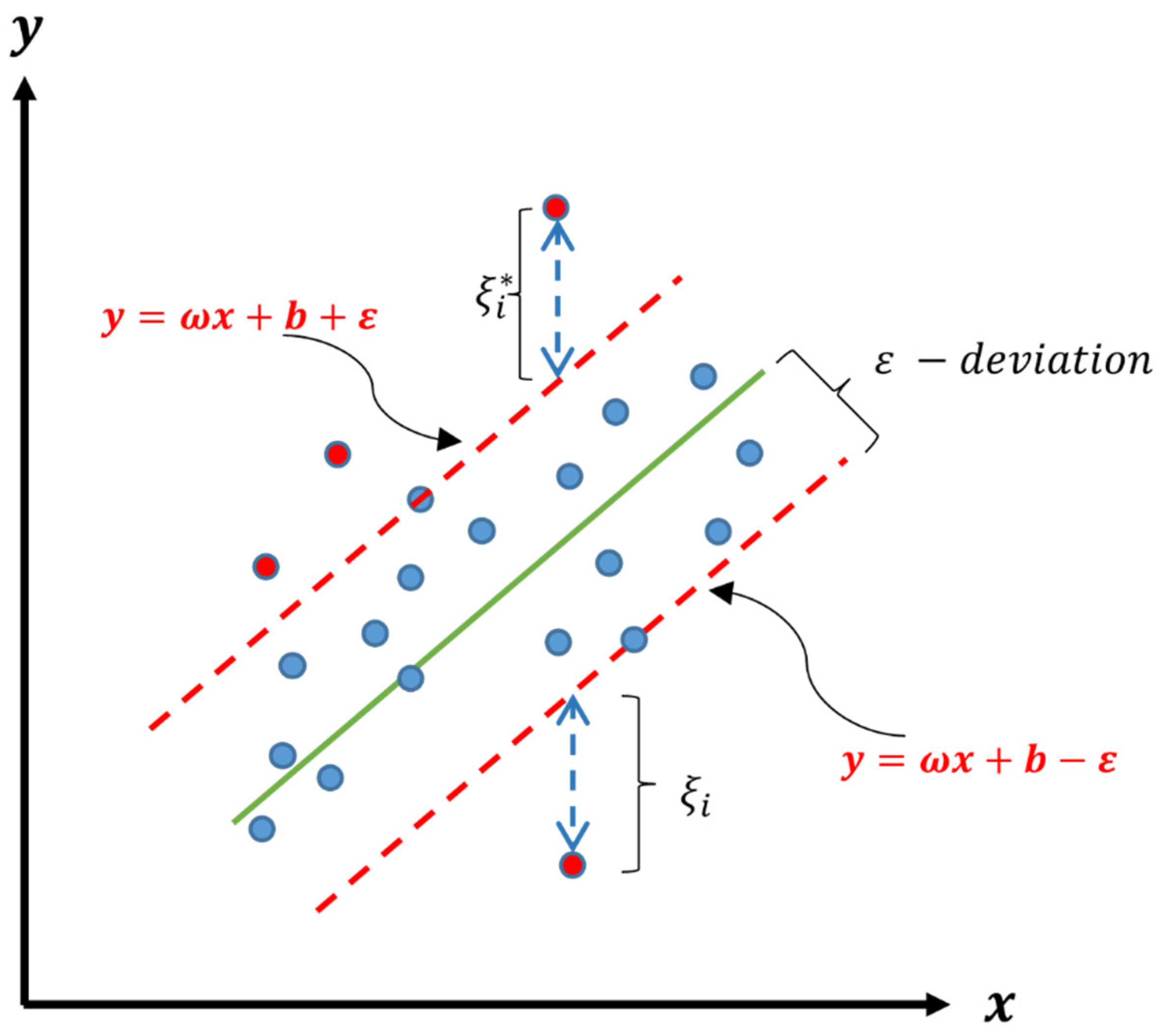
2.3.1. Support Vector Regression

Support Vector Machines (SVM), as a kind of machine learning method, are widely used in classification problems. Support Vector Regression (SVR) as defined by Drucker, et al. [30] uses the same principle as SVM, but for regression problems, not classification. The regression problem is to find a function that can generate values close to the response variable values corresponding to a set of inputs based on a data pattern [31]. SVR is an algorithm that allows decision-makers to choose tolerances for errors through both a satisfactory margin of error (ϵ) and an acceptance adjustment, thus providing flexibility for them [32]. Contrary to the ordinary least square method, the objective function of SVR is to minimize the coefficients—more specifically, the l2-norm of the coefficient vector—instead of the squared error. The objective function and constraints of SVR can be given as follows:
m i n i m i z e 1 2 w 2 s u b j e c t   t o   | y i ( w i x i b ) | ε              
An illustrative example of simple SVR in a regression problem is given in Figure 2.

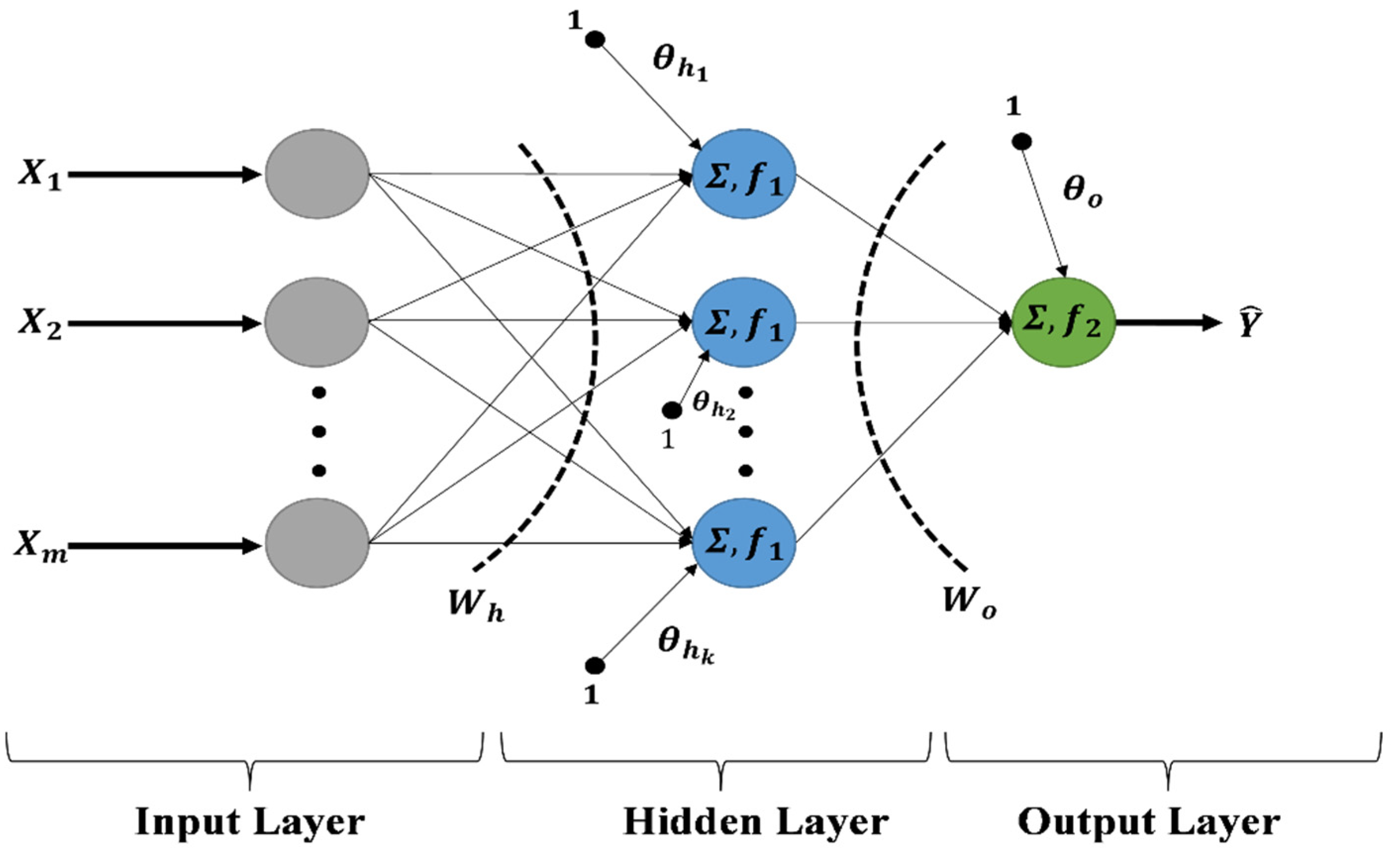
2.3.2. Feed Forward Neural Networks

Artificial neural networks (ANNs) have the ability to create and discover new knowledge through learning, which is one of the characteristics of the human brain thanks to the talent to use supervised and unsupervised machine learning algorithms. Multi-layer perceptron (MLP), introduced by Werbos [33] and improved by Rumelhart, et al. [34], is widely used to solve nonlinear problems. MLP consists of three main layers as an input, an output layer, and one or more hidden layers. While the number of units of the input layer is determined based on the dimension of the input data, the number of neurons in the output layer depends on the response variables. FFNN is a multilayer perceptron class of ANNs. Since the experimental design problem focused in this study is essentially a regression problem, a feedforward neural network (FFNN) using supervised learning is preferred. Figure 3 presents a hypothetical FFNN architecture with m input layer units and o n e output layer unit. For this hypothetical architecture, there are k units in the hidden layer.
Here X 1 , X 2 , , X m form the input of FFNN as a learning sample. Y ^ is the output of the neural network and represents the prediction of the response variable. The W h matrix is the weights as an indicator of the contribution of the input units to the hidden layer units. W o vector is the weights as an indicator of the contribution of the hidden layer units to the output layer. Moreover, θ h and θ o represent the biases for the hidden layer units and the output layer unit, respectively. The Σ symbol in both the hidden and the output layers indicates an additive aggregation function. Moreover, f 1 and f 2 are the activation functions used in the hidden layer and the output layer, respectively.

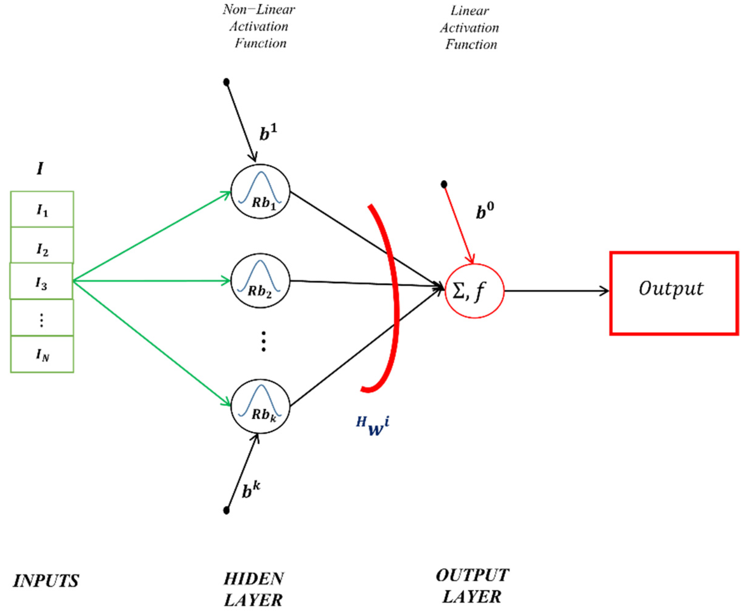
2.3.3. Radial Basis Function Networks

BFFs are another commonly used ANN for regression problems as a function approximation tool [35]. Although RBFNs are similar to a conventional multilayer perceptron (MLP) with their basic structure, they also have some remarkable characteristics that distinguish them from others. Similar to classical MLP, the architecture of RBFNs consists of three layers; the input layer, the hidden layer, and the output layer. The major discrepancy of the RBFNs from classical MLP is that RBFNs can provide a non-linear transformation of the input space without weights in the hidden layer [36,37]. The hidden layer units called the radial basis function are determined by two parameters, the centre and the width [38,39]. Figure 4 shows a hypothetical RBFN architecture structure.
Here, I = [ I 1   I 2     I N ] is a input vector. R b i , i = 1 , k ¯ is i th radial basis in the hidden layer and b i is bias for i th radial basis. w i H is the weight between i th radial basis and the output layer neuron ( i = 1 , k ¯ ) . The output of i th radial basis is calculated as in Equation (2).
R b i o = e x p ( I c i 2 σ i 2 ) ; i = 1 , k ¯
Here, . is the Euclidean norm. c i and σ i are the centre and the width of the i th radial basis, respectively. So, the output of the RBFN is obtained by using following equations.
n e t = i = 1 k R b i o w i H
O u t p u t = f ( n e t ) = n e t

2.4. Modelling the Treatment Process

In this study, machine learning-based methods have been used to model the treatment of landfill leachate performed by c-Fenton and p-Fenton processes. Thus, it is realized the prediction the main factors in the removal performance of both Fenton processes for the treatment of landfill leachate. The SVR, the FFNN and the RBFNN, in this direction, have been utilized. The datasets of each experiment, as training, validation and testing, have been divided into three subsets. The learning process, using the training set, is carried out for different hyperparameters, while the hyperparameters with the best learning, with the validation set, are specified. The test set gives a performance measure of the trained method for out-of-sample data points. Moreover, in order to evaluate the ML-based methods with a statistical method, the RSM was also applied for each of the experiments. The processes of the analysis and the modelling used ML-based methods were performed with the MATLAB R2018b program codes created by researchers. Table 2 presents the summary information on all experiments for the classical and the p-Fenton processes.

Evaluation Perspectives

This study comprises different perspectives for a detailed evaluation of the obtained results.
Comparative evaluation in terms of error metrics: root mean square error (RMSE) and mean absolute percentage error (MAPE) have been used for this purpose.
RMSE = 1 n p = 1 n ( Target p Output p ) 2
MAPE = mean ( | Target p Output p Target p | ) ,   p = 1 , 2 , , n
Here, Target p and Output p , for p th observations of the experiment, represent the observed real values or desired values and the predicted values or output of the modelling tool, respectively.
To examine model fit, regression analysis and its characteristics are applied.
Y p = β Y ^ p + ε p
The determination and the regression coefficients, obtained from the regression model given in Equation (7), for a preferable estimator, should be equal to 1 or very close to 1.
Presentation of graphs with values for the predicted and observed response variables serve as fit demonstrations.

3. Results and Discussion

3.1. Evaluation of the Results in Comparison with the Error Criteria

Table S1 (supplementary data) shows the model performances in terms of RMSE. The results presented in Table S1 show that the RBFN and the FFNN, for all experiments, compared to RSM and other ML-based methods SVR, have superior predictive and modelling abilities. These figures indicate that the RBFN delivers outstanding performance considering all experiments. In addition, the same results were obtained in Table S2, where the modelling performances of the methods are presented in terms of the MAPE criterion. For all experiments, the RBFN and the FFNN have in particular displayed exceptional prediction capabilities.Considering the average rank values as a measure of the degree of success, it is clearly seen that the RBFNN has the best performance for all data sets. The RBFNN has an average rank value of 1.2 for the training set. This average figure, the validation and the testing sets, are 1.1 and 2.1, respectively. The average rankings have been recorded as 1.1 and 2.1, respectively, for the validation and the testing sets. The RBFN again has the lowest mean ranking with a value of 1.6 for the whole dataset.
From another aspect, when MAPE values, which are a percentile error measure independent of the unit of the data set, are evaluated alone, both the FFNN and the RBFNN have revealed percentile errors very close to zero. This is further proof of the superior modelling performance of these ML-based methods.

3.2. Examining Model Fit: Regression Analysis and Using Some of Its Features

The coefficient of determination ( R 2 ) and the regression coefficient ( β ^ ) obtained from linear regression analysis can also be used as a measure of model fit. For a reasonable model fit, from the simple linear regression model of Y t = β Y ^ t + ε t , the values of β ^ and also the determination coefficient R 2 should be estimated as 1 or very close to 1. At this stage, the focus is on the model fit success of the RBFN, as it performs best for almost all experiments and datasets. Table 3 summarizes the relevant findings.
Table S2 presents the findings that indicate that the RBFNN has produced predictions that are highly consistent with the observed cure rate. These findings show that both β and R 2 values, as expected, have been obtained pretty close to 1. It should be noted that when compared to the outcomes of studies in the same field published in the literature in recent years, the model utilized in this study produces more accurate predictions [40,41]. Also, for all experiments, the 95% confidence intervals of the beta are both very narrow and cover 1. This indicates a perfect model fit. Thus, on the basis of all these findings obtained from regression analysis, it can be said that the RBFN is an extraordinary ML-based method for modelling the removal ratio.

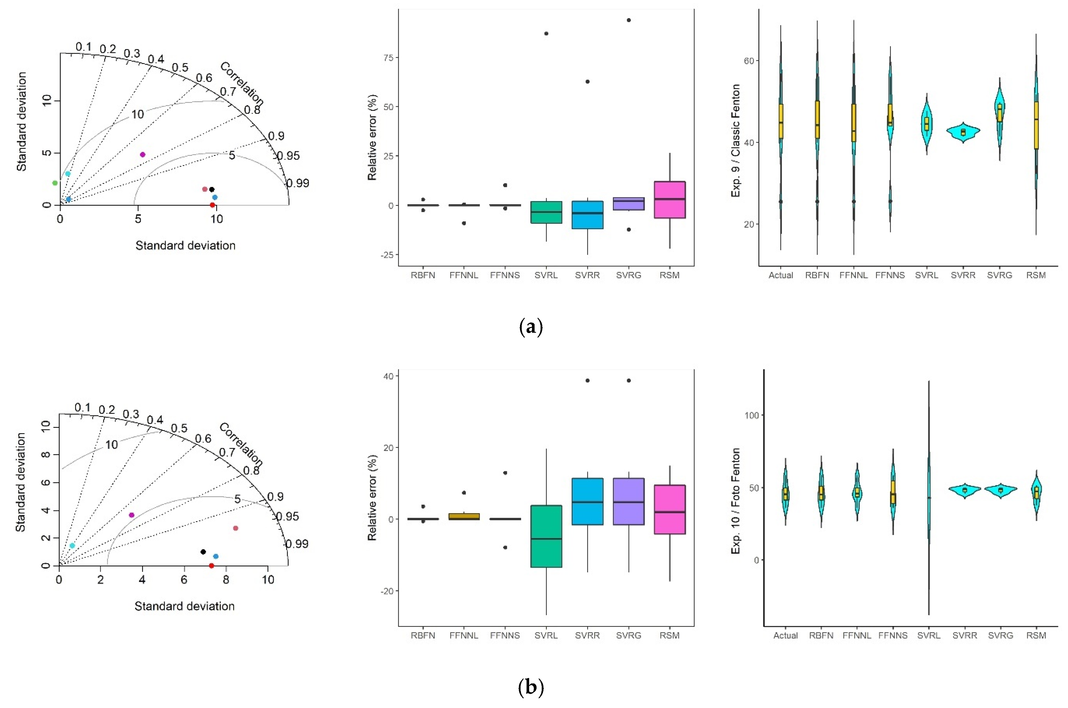
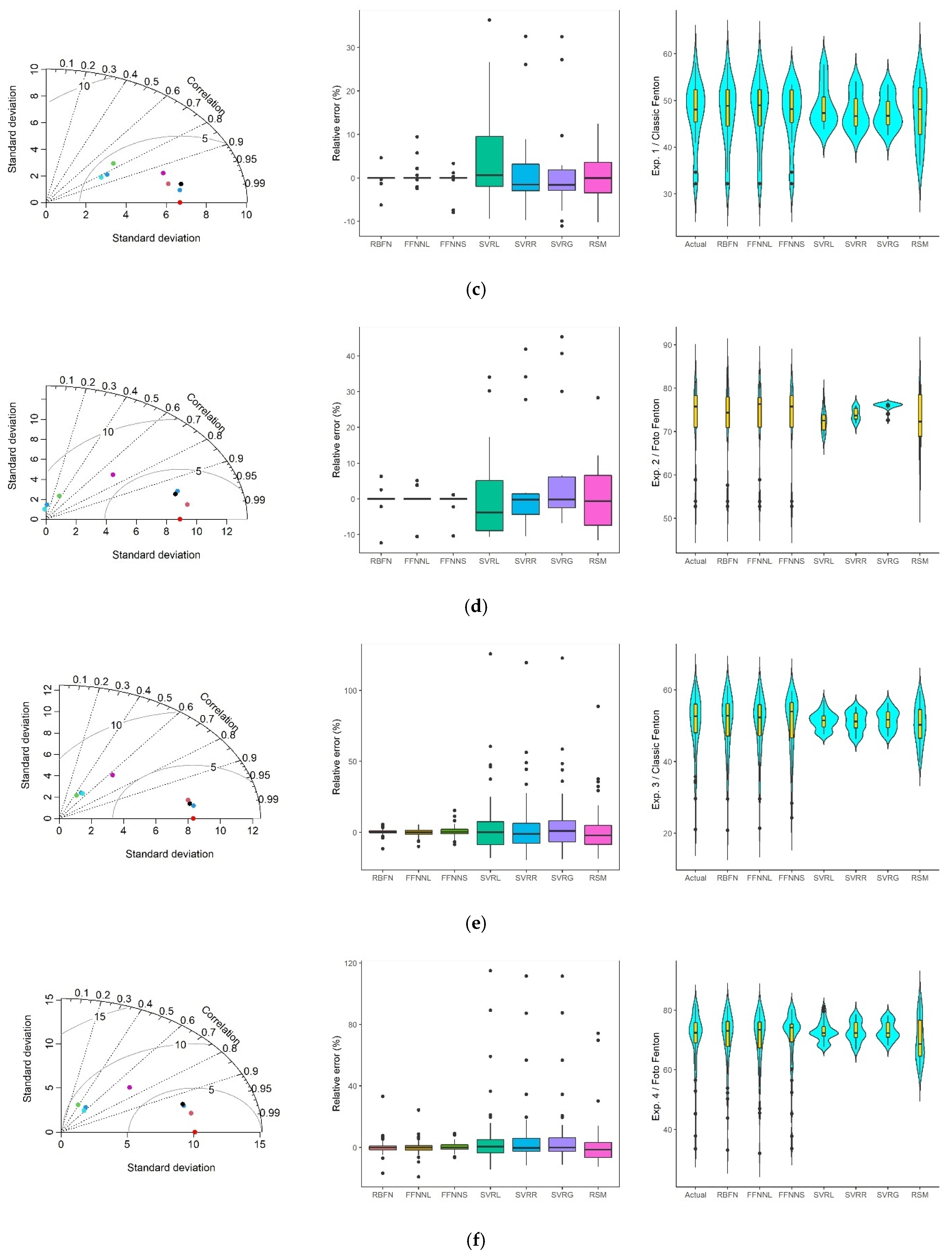
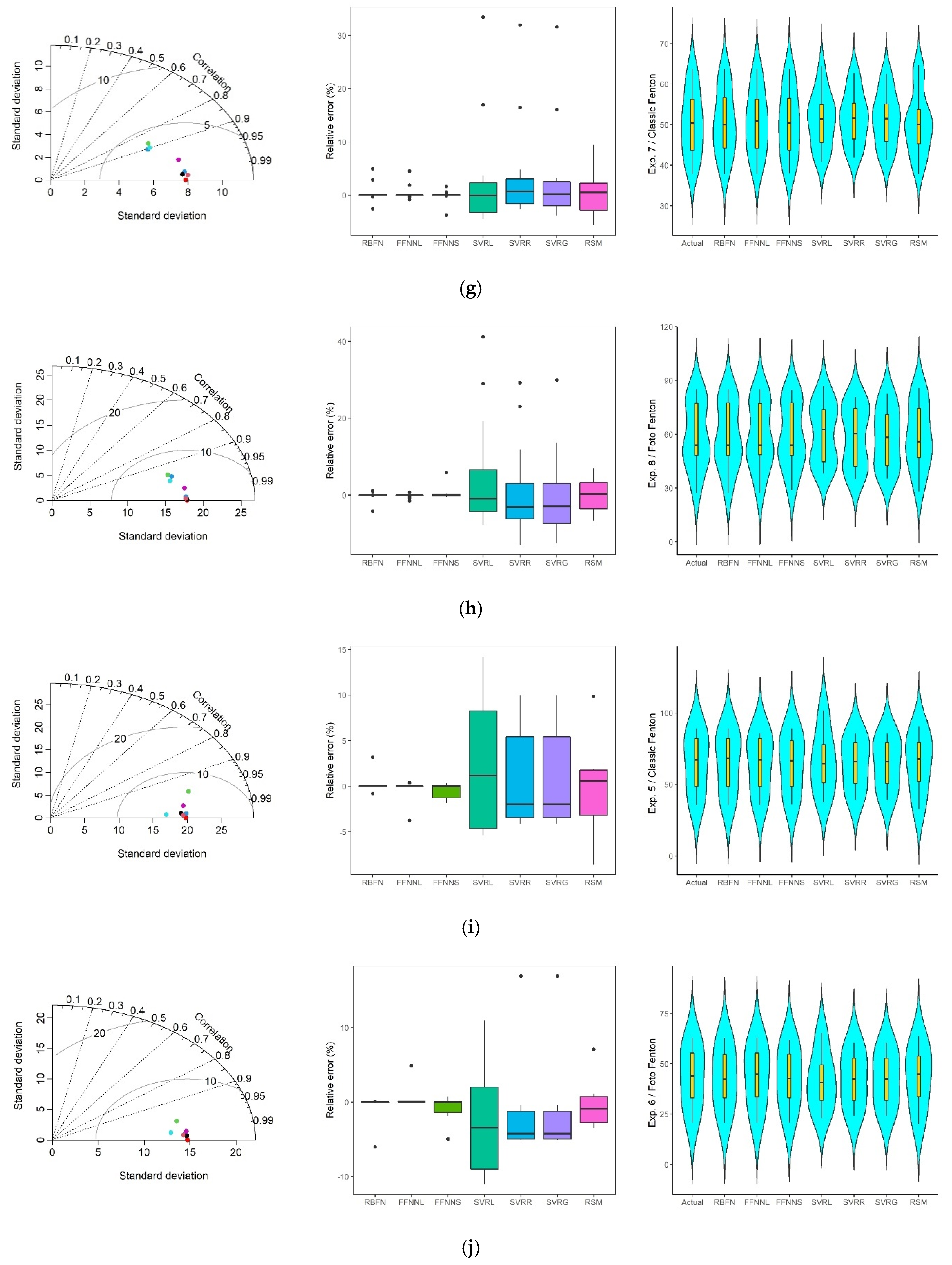
3.3. Interpreting Some Visuals: Scatter Plots and Some Typical Graphs

For most of the analysis of the datasets, the RBFN had the best or sufficiently satisfactory modelling performances comparing the other ML-based modelling tools and the RSM. For this reason only, we have preferred to use the RBFN results to investigate model fit by way of scatter plots. Figure S1 presents a visual perspective of the outstanding performance of the RBFN and high harmony between the predicted and observed removal rates. The proof of this fact, as expected, is that almost all points are on the line segment.
Moreover, with some typical graphs given in Figure 5, all of these findings have been supported. The first is the Taylor diagram which presents the standard deviations (SDs) besides correlations between the observed and the predicted values. Taylor diagrams show that the standard deviations of the predictions of the RBFN (pink points) are quite close to the SDs of the observed removal rates. Also, the FFNN (blue and black points) which is another ML-based method, also marked close points with the RBFN (pink points) for all experiments. Another typical graph is the box plot that indicates the modelling capability of the methods in terms of reliability and validity. The box plots for all experiments showed that the RBFN and the FFNN produced pretty reliable and invariant modelling results. Finally, the violin plots were given as a visual measure of harmony of distribution of the observed and predicted values presented. The violin plots clearly show that the predicted values distribution of the RBFN and the FFNNs, compared with the other modelling methods, are remarkably in agreement with the distribution of the observed values. The first is the Taylor diagram, which can be used to graphically summarise how close a set of patterns (in this case, a collection of models) match observations. Taylor diagrams provide “a concise statistical summary of how well patterns match each other in terms of their correlation, their root-mean-square difference or the ratio of their variances. Here, it presents the standard deviations (SDs) besides correlations between the observed and the predicted values. Taylor diagrams show that the standard deviations of the predictions of the RBFN (pink points) are quite close to the SDs of the observed removal rates. Also, the FFNN (blue and black points) which is another ML-based method, also marked close points with the RBFN (pink points) for all experiments. Another typical graph is the box plot that visually shows the distribution of numerical data and skewness by displaying the data quartiles (and percentiles) and averages. Box plots show the five-number summary of a set of data: including the minimum score, first (lower) quartile, median, third (upper) quartile, and maximum score. The box plot also indicates the modelling capability of the methods in terms of reliability and validity. The box plots for all experiments showed that the RBFN and the FFNN produced pretty reliable and invariant modelling results. Finally, a violin plot is a hybrid of a box plot and a kernel density plot, which shows peaks in the data. It is used to visualize the distribution of numerical data. Unlike a box plot that can only show summary statistics, violin plots depict summary statistics and the density of each variable. Wider sections of the violin plot represent a higher probability that members of the population will take on the given value; the skinnier sections represent a lower probability. The violin plots were given as a visual measure of harmony of distribution of the observed and predicted values that were presented. The violin plots clearly show that the predicted values distribution of the RBFN and the FFNNs, compared with the other modelling methods, are remarkably in agreement with the distribution of the observed values.

3.4. Optimization of the Parameters

The modelling process of the treatment of landfill leachate can be counted as a suitable function finding process for the experiments. The inputs of this function consist of the parameters of the treatment process, while the output is the removal ratio. This section of the article concentrates on determining the optimal values of the parameters to maximize removal ratios by GA using estimated functions. The importance of optimization is that new experiments are not required to conduct further investigations. Trained RBFN has been used at this stage since it has impressive modelling capability. Specifically, an maximation problem with N decision variables and J + K constraints can be established as follows.
m a x ( f ( x _ ) ) ( x _ = [   x 1   x 2     x N ] ) subject   to   g j ( x _ ) 0 ; j = 1 , 2 , , J h k ( x ) = 0 ; k = 1 , 2 , , K x i ( L ) x i x i ( L ) ; i = 1 , 2 , , N
GA, an adaptive heuristic search algorithm based on the concept of survival of the fittest, was used in the optimization.
The desirability coefficient given in Equation (9) can be used as a measure of optimization performance. Here, M i n and M a x represent the limit value of the dependent variables.
d m a x = { 0 ;   f ( x _ ) < M i n   ( f ( x _ ) M i n   M a x M i n   ) ; M i n < f ( x _ ) < M a x 1 ; f ( x _ ) > M a x }
For each experiment, summary information and results of the optimization process are given in Table 4. From the figures given in Table 4, with 100.00%, extraordinary desirability levels were achieved for all experiments, with the exception of only two experiments where desirability levels are still about 100.00% (99.99%). Table 4 also shows that p-Fs have higher treatment performance than c-Fs in each experiment, except in one, under the optimum conditions.
The maximum removal efficiency was found in pH 3.0, and the removal efficiency in both processes decreased as the pH increased. This situation indicated that the increasing free radicals in acidic conditions increased the oxidation of organic substances.
With higher reagent dosages for both Fenton procedures, the removal efficiencies increased. The Fenton process is sensitive to the concentration of ferrous ions, and as FeSO4 concentration rises, more pollutants are removed. Moreover, the improvement of the pollutant removal with an increase in H2O2 concentration is due to the augmentation of the hydroxyl radicals. As seen in Table 4, the difference between the removal efficiencies increased from 110.5 mg L−1 of Fe2+ dose. By the increase of Fe2+ dose from 192.4 to 290.4 mg L−1, the removal efficiencies in the p-Fenton oxidation increased from 82 to 85%. According to the results from the p-Fenton experiments, it was found that the increase in the H2O2 dose had no significant effect on COD removal efficiency. Here, the interaction of hydroxyl radicals with H2O2, which enhances the OH˚ scavenging capability at high H2O2 concentrations, and hydroxyl radical recombination can be shown to be the cause of the decrease in COD removal efficiency.
At the end of 60 min, the maximum removal efficiencies were found to be 63% for the c-Fenton, and 85% for the p-Fenton. When the experimental findings were analyzed, it was found that p-Fenton accomplished roughly 75% removal in the first 15 min as opposed to c-Fenton’s 50% removal in the same time frame. At the end of the first 30 min, both procedures had achieved COD removal efficiency rates of roughly 60% in c-Fenton and approximately 80% in p-Fenton. Aside from that, the model findings showed that the COD removal for c-Fenton could not reach 63% after 36 min based on the contact duration of 1 h in both oxidations, and that a considerable COD removal of 85% at the end of 50 min for p-Fenton was achieved. This instance demonstrates the gradual increase in COD’s removal efficiency. Further irradiation duration exceeding 25 min, however, does not significantly benefit the treatment. It should be noted that during the first 30 min, p-Fenton had removed almost 80% of the COD; there was thereafter a continual but diminishing acceleration of removal; and only a 5% increase was observed during the following 20 min. Looking at the optimization model results of the effectiveness of the number of UV lamps on the treatment efficiency in p-Fenton, it is seen that there is an increase from 62% to 82% under 8 UV lamps compared to 7 UV lamps. The circumstances that achieved the highest removal efficiency, meanwhile, might not be ideal for operational use, since the system’s cost is likewise significant.

4. Conclusions

In this study, ML-based modelling methods were used to predict c-Fenton and p-Fenton processes in the treatment of landfill leachate. In the stage of experimental design, four experiments were organized for both Fenton processes. In the modelling stage, the RBFN, the FFNN, and the SVR were used and the results were evaluated in a broad scanning. In the analyses at this stage, the data sets that make up the experiments are divided into three parts: training, validation and testing. Another remarkable characteristic of this study is that the input parameters of the processes are optimized with GA. When the results are considered as a whole, it has been observed that the superior-modelling capabilities of ML-based models, especially the RBFN and the FFNN, came to the fore. Accordingly, this study confirmed the potential use of the ML-based modeling tool for landfill leachate treatment by sustainable optimization of p-Fenton processes. In addition to evaluating modelling performance, by optimizing the parameters of Fenton processes, optimum conditions were determined that will maximize the removal performance without the need for extra experiments. One of the most significant results of the experiment was that, based on how both processes functioned after the first 30 min, COD removal efficiency rates of around 60% in c-Fenton and roughly 80% in p-Fenton were attained.. The effective contact times with the highest efficiency were determined as 64% efficiency at 36 min and 85% efficiency at 50 min for c-Fenton and p-Fenton processes, respectively. By the application of UV radiation to the Fenton oxidation, the removal efficiency increased about 20% due to increased •OH. Moreover, it has been observed that the p-Fenton process performs better than the c-Fenton process in the treatment of landfill leachate under optimum conditions.
It might be conceivable to totally treat the leachate in line with the discharge standards by offering sustainable optimization of the ML-based model through similar applications. To provide greater performance, optimization algorithms are frequently researched for novel materials, approaches, workflows, and combinations. In order to stop the environmental damage produced by these wastewaters, several treatment techniques can also be combined to boost treatment performance, and the treated water can be reused. Considering this, the authors propose that future study on this topic might include the sustainable optimization of a number of pre-treatment techniques (such as adsorption and coagulation) before treating leachate with AOP.

Supplementary Materials

The following supporting information can be downloaded at: https://0-www-mdpi-com.brum.beds.ac.uk/article/10.3390/su141811261/s1, Figure S1. The scatter plots of the observed and the predicted parameters for the RBFN. Table S1. The modelling results in terms of RMSE. Table S2. The modelling results in terms of MAPE.

Author Contributions

H.C.: Supervision, conceptualization and methodology, writing-original draft, visualization, writing & review and editing. D.Ö.: Investigation, performed the experiments, data curation, validation, writing & review and editing. All authors have read and agreed to the published version of the manuscript.

Funding

This research received no external funding.

Institutional Review Board Statement

Not applicable.

Informed Consent Statement

Not applicable.

Data Availability Statement

All data produced or analyzed during this study is included in this article.

Acknowledgments

The authors would like to thank the Municipality of Sivas (Türkiye) for enabling us to supply landfill leachate during the thesis study. In addition, the authors are thanking and feel grateful to Nevşehir Haci Bektaş Veli University (Türkiye), Department of Environmental Engineering for their laboratory support.

Conflicts of Interest

The authors declare that they have no conflicts of interest.

References

  1. Shaban, A.; Zaki, F.-E.; Afefy, I.H.; Di Gravio, G.; Falegnami, A.; Patriarca, R. An Optimization Model for the Design of a Sustainable Municipal Solid Waste Management System. Sustainability 2022, 14, 6345. [Google Scholar] [CrossRef]
  2. Tejera, J.; Gascó, A.; Hermosilla, D.; Alonso-Gomez, V.; Negro, C.; Blanco, Á. Uva-led technology’s treatment efficiency and cost in a competitive trial applied to the photo-fenton treatment of landfill leachate. Processes 2021, 9, 1026. [Google Scholar] [CrossRef]
  3. Luo, H.; Zeng, Y.; Cheng, Y.; He, D.; Pan, X. Recent advances in municipal landfill leachate: A review focusing on its characteristics, treatment, and toxicity assessment. Sci. Total Environ. 2020, 703, 135468. [Google Scholar] [CrossRef] [PubMed]
  4. Reshadi, M.A.M.; Bazargan, A.; McKay, G. A review of the application of adsorbents for landfill leachate treatment: Focus on magnetic adsorption. Sci. Total Environ. 2020, 731, 138863. [Google Scholar] [CrossRef]
  5. Tejera, J.; Miranda, R.; Hermosilla, D.; Urra, I.; Negro, C.; Blanco, Á. Treatment of a mature landfill leachate: Comparison between homogeneous and heterogeneous photo-Fenton with different pretreatments. Water 2019, 11, 1849. [Google Scholar] [CrossRef]
  6. Dantas, E.R.; Silva, E.J.; Lopes, W.S.; do Nascimento, M.R.; Leite, V.D.; de Sousa, J.T. Fenton treatment of sanitary landfill leachate: Optimization of operational parameters, characterization of sludge and toxicology. Environ. Technol. 2020, 41, 2637–2647. [Google Scholar] [CrossRef]
  7. Temel, F.A.; Yolcu, Ö.C.; Kuleyin, A. A multilayer perceptron-based prediction of ammonium adsorption on zeolite from landfill leachate: Batch and column studies. J. Hazard. Mater. 2021, 410, 124670. [Google Scholar] [CrossRef]
  8. Mahtab, M.S.; Islam, D.T.; Farooqi, I.H. Optimization of the process variables for landfill leachate treatment using Fenton based advanced oxidation technique. Eng. Sci. Technol. Int. J. 2021, 24, 428–435. [Google Scholar] [CrossRef]
  9. Amor, C.; De Torres-Socías, E.; Peres, J.A.; Maldonado, M.I.; Oller, I.; Malato, S.; Lucas, M.S. Mature landfill leachate treatment by coagulation/flocculation combined with Fenton and solar photo-Fenton processes. J. Hazard. Mater. 2015, 286, 261–268. [Google Scholar] [CrossRef]
  10. Poblete, R.; Pérez, N. Use of sawdust as pretreatment of photo-Fenton process in the depuration of landfill leachate. J. Environ. Manag. 2020, 253, 109697. [Google Scholar] [CrossRef]
  11. Alavi, N.; Dehvari, M.; Alekhamis, G.; Goudarzi, G.; Neisi, A.; Babaei, A.A. Application of electro-Fenton process for treatment of composting plant leachate: Kinetics, operational parameters and modeling. J. Environ. Health Sci. Eng. 2019, 17, 417–431. [Google Scholar] [CrossRef] [PubMed]
  12. Renou, S.; Givaudan, J.; Poulain, S.; Dirassouyan, F.; Moulin, P. Landfill leachate treatment: Review and opportunity. J. Hazard. Mater. 2008, 150, 468–493. [Google Scholar] [CrossRef] [PubMed]
  13. Zazouli, M.A.; Yousefi, Z.; Eslami, A.; Ardebilian, M.B. Municipal solid waste landfill leachate treatment by fenton, photo-fenton and fenton-like processes: Effect of some variables. Iran. J. Environ. Health Sci. Eng. 2012, 9, 3. [Google Scholar] [CrossRef] [PubMed]
  14. Welter, J.B.; Soares, E.V.; Rotta, E.H.; Seibert, D. Bioassays and Zahn-Wellens test assessment on landfill leachate treated by photo-Fenton process. J. Environ. Chem. Eng. 2018, 6, 1390–1395. [Google Scholar] [CrossRef]
  15. Abiodun, O.I.; Jantan, A.; Omolara, A.E.; Dada, K.V.; Mohamed, N.A.; Arshad, H. State-of-the-art in artificial neural network applications: A survey. Heliyon 2018, 4, e00938. [Google Scholar] [CrossRef]
  16. Geyikçi, F.; Kılıç, E.; Çoruh, S.; Elevli, S. Modelling of lead adsorption from industrial sludge leachate on red mud by using RSM and ANN. Chem. Eng. J. 2012, 183, 53–59. [Google Scholar] [CrossRef]
  17. Değermenci, N.; Akyol, K. Decolorization of the Reactive Blue 19 from aqueous solutions with the Fenton oxidation process and modeling with deep neural networks. Water Air Soil Pollut. 2020, 231, 72. [Google Scholar] [CrossRef]
  18. Raji, M.; Tahroudi, M.N.; Ye, F.; Dutta, J. Prediction of heterogeneous Fenton process in treatment of melanoidin-containing wastewater using data-based models. J. Environ. Manag. 2022, 307, 114518. [Google Scholar] [CrossRef]
  19. Hosseinzadeh, A.; Najafpoor, A.A.; Navaei, A.A.; Zhou, J.L.; Altaee, A.; Ramezanian, N.; Dehghan, A.; Bao, T.; Yazdani, M. Improving Formaldehyde Removal from Water and Wastewater by Fenton, Photo-Fenton and Ozonation/Fenton Processes through Optimization and Modeling. Water 2021, 13, 2754. [Google Scholar] [CrossRef]
  20. Cüce, H.; Temel, F.A.; Yolcu, O.C. Modelling and optimization of Fenton processes through neural network and genetic algorithm. Korean J. Chem. Eng. 2021, 38, 2265–2278. [Google Scholar] [CrossRef]
  21. Kanafin, Y.N.; Makhatova, A.; Zarikas, V.; Arkhangelsky, E.; Poulopoulos, S.G. Photo-Fenton-like treatment of municipal wastewater. Catalysts 2021, 11, 1206. [Google Scholar] [CrossRef]
  22. Gomes, R.K.; Santana, R.M.; de Moraes, N.F.; Júnior, S.G.S.; de Lucena, A.L.; Zaidan, L.E.; Elihimas, D.R.; Napoleao, D.C. Treatment of direct black 22 azo dye in led reactor using ferrous sulfate and iron waste for Fenton process: Reaction kinetics, toxicity and degradation prediction by artificial neural networks. Chem. Pap. 2021, 75, 1993–2005. [Google Scholar] [CrossRef]
  23. Varank, G.; Yazici Guvenc, S.; Dincer, K.; Demir, A. Concentrated leachate treatment by electro-fenton and electro-persulfate processes using central composite design. Int. J. Environ. Res. 2020, 14, 439–461. [Google Scholar] [CrossRef]
  24. Rashid, A.; Mirza, S.A.; Keating, C.; Ijaz, U.Z.; Ali, S.; Campos, L.C. Machine Learning Approach to Predict Quality Parameters for Bacterial Consortium-Treated Hospital Wastewater and Phytotoxicity Assessment on Radish, Cauliflower, Hot Pepper, Rice and Wheat Crops. Water 2022, 14, 116. [Google Scholar] [CrossRef]
  25. Biglarijoo, N.; Mirbagheri, S.A.; Bagheri, M.; Ehteshami, M. Assessment of effective parameters in landfill leachate treatment and optimization of the process using neural network, genetic algorithm and response surface methodology. Process Saf. Environ. Prot. 2017, 106, 89–103. [Google Scholar] [CrossRef]
  26. Thind, P.S.; John, S. Optimizing the Fenton based pre-treatment of landfill leachate using response surface methodology. J. Water Chem. Technol. 2020, 42, 275–280. [Google Scholar] [CrossRef]
  27. Yang, J.; Jia, J.; Wang, J.; Zhou, Q.; Zheng, R. Multivariate optimization of the electrochemical degradation for COD and TN removal from wastewater: An inverse computation machine learning approach. Sep. Purif. Technol. 2022, 295, 121129. [Google Scholar] [CrossRef]
  28. Di Franco, G.; Santurro, M. Machine learning, artificial neural networks and social research. Qual. Quant. 2021, 55, 1007–1025. [Google Scholar] [CrossRef]
  29. Yolcu, O.C.; Temel, F.A.; Kuleyin, A. New hybrid predictive modeling principles for ammonium adsorption: The combination of Response Surface Methodology with feed-forward and Elman-Recurrent Neural Networks. J. Clean. Prod. 2021, 311, 127688. [Google Scholar] [CrossRef]
  30. Drucker, H.; Burges, C.J.; Kaufman, L.; Smola, A.; Vapnik, V. Support vector regression machines. Adv. Neural Inf. Process. Syst. 1996, 9, 155–161. [Google Scholar]
  31. Babbar, N.; Kumar, A.; Verma, V.K. Crop management: Wheat yield prediction and disease detection using an intelligent predictive algorithms and metrological parameters. In Deep Learning for Sustainable Agriculture; Elsevier: Amsterdam, The Netherlands, 2022; pp. 273–295. [Google Scholar]
  32. Helman, D.; Lensky, I.M.; Bonfil, D.J. Early prediction of wheat grain yield production from root-zone soil water content at heading using Crop RS-Met. Field Crops Res. 2019, 232, 11–23. [Google Scholar] [CrossRef]
  33. Werbos, P.J. The Roots of Backpropagation: From Ordered Derivatives to Neural Networks and Political Forecasting; John Wiley & Sons: Hoboken, NJ, USA, 1994; Volume 1. [Google Scholar]
  34. Rumelhart, D.E.; Hinton, G.E.; Williams, R.J. Learning Internal Representations by Error Propagation; California University San Diego La Jolla Institute for Cognitive Science: San Diego, CA, USA, 1985. [Google Scholar]
  35. Sharifahmadian, A. Numerical Models for Submerged Breakwaters: Coastal Hydrodynamics and Morphodynamics; Butterworth-Heinemann: Oxford, UK, 2015. [Google Scholar]
  36. Faris, H.; Aljarah, I.; Mirjalili, S. Evolving radial basis function networks using moth–flame optimizer. In Handbook of Neural Computation; Elsevier: Amsterdam, The Netherlands, 2017; pp. 537–550. [Google Scholar]
  37. Hamedi, S.; Kordrostami, Z.; Yadollahi, A. Artificial neural network approaches for modeling absorption spectrum of nanowire solar cells. Neural Comput. Appl. 2019, 31, 8985–8995. [Google Scholar] [CrossRef]
  38. Al-Amoudi, A.; Zhang, L. Application of radial basis function networks for solar-array modelling and maximum power-point prediction. IEE Proc.-Gener. Transm. Distrib. 2000, 147, 310–316. [Google Scholar] [CrossRef]
  39. Chuang, C.-C.; Jeng, J.-T.; Lin, P.-T. Annealing robust radial basis function networks for function approximation with outliers. Neurocomputing 2004, 56, 123–139. [Google Scholar] [CrossRef]
  40. Maslahati Roudi, A.; Chelliapan, S.; Wan Mohtar, W.H.M.; Kamyab, H. Prediction and optimization of the fenton process for the treatment of landfill leachate using an artificial neural network. Water 2018, 10, 595. [Google Scholar] [CrossRef]
  41. Amiri, A.; Sabour, M.R. Multi-response optimization of Fenton process for applicability assessment in landfill leachate treatment. Waste Manag. 2014, 34, 2528–2536. [Google Scholar] [CrossRef]
Figure 1. A representation of p-Fenton cabin.
Sustainability 14 11261 g001
Figure 2. An example illustration of the one-dimensional SVR model.
Sustainability 14 11261 g002
Figure 3. A hypothetical architecture of the FF-NN [29].
Sustainability 14 11261 g003
Figure 4. A hypothetical architecture of the RBFNs.
Sustainability 14 11261 g004
Figure 5. The visual assessment of the predictors’ performance. (a) Experiment 1-Classic Fenton. (b) Experiment 2-Photo Fenton. (c) Experiment 3-Classic Fenton. (d) Experiment 4-Photo Fenton. (e) Experiment 5-Classic Fenton. (f) Experiment 6-Photo Fenton. (g) Experiment 7-Classic Fenton. (h) Experiment 10-Photo Fenton. (i) Experiment 8-Photo Fenton. (j) Experiment 9-Photo Fenton.
Sustainability 14 11261 g005aSustainability 14 11261 g005bSustainability 14 11261 g005c
Table 1. The characterization of the landfill leachate.
ParametersValues
COD (mg L−1)4671
pH6.9
Electrical conductivity (µS cm−1)6200
Ortho-phosphate (mg L−1 PO4−2)9.6
Sulfate (mg L−1 SO4−2)478
Table 2. The summary of experiments and architectures of the MLP.
Expr.
No
Treatment ProcessIndependent VariablesFixed VariablesThe # of
Data Set
1c-FentonA. pH (2–7)1. Temperature/23 ± 2°C
2. Fast/slow mixing speed/400–90 rpm
3. Fe(II)/H2O2 = (300/2000) mg/L dose
4. Process duration/60 min
Training—2
Validation—2
Testing—2
2p-FentonA. pH (2–7)1. Temperature/23 ± 2°C
2. Fast/slow mixing speed/400–90 rpm
3. Fe(II)/H2O2 = (300/2000) mg/L dose
4. Process duration /60 min
5. Light intensity/8 lamps/64 Watt
Training—2
Validation—2
Testing—2
3c-FentonA. Fe (II) dose (50–400 mg/L)
B. H2O2 dose (1000, 2000 mg/L)
1. pH/3 ± 0.2
2. Temperature/23 ± 2°C
3. Fast/slow mixing speed/400–90 rpm
Training—8
Validation—4
Testing—4
4p-FentonA. Fe (II) dose (50–400 mg/L)
B. H2O2 (1000, 2000 mg/L)
1. pH/3 ± 0.2
2. Temperature/23 ± 2°C
3. Fast/slow mixing speed/400–90 rpm
4. Light intensity/8 lamps/64 Watt
Training—8
Validation—4
Testing—4
5c-FentonA. H2O2 dose (100–3000 mg/L)
B. Fe (II) dose (150, 300, 400 mg/L)
1. pH/3 ± 0.2
2. Temperature/23 ± 2°C
3. Fast/slow mixing speed/400–90 rpm
Training—31
Validation—10
Testing—10
6p-FentonA. H2O2 dose (100–3000 mg/L)
B. Fe (II) dose (100, 125, 300 mg/L)
1. pH/3 ± 0.2
2. Temperature/23 ± 2°C
3. Fast/slow mixing speed/400–90 rpm
4. Light intensity/8 lamps/64 Watt
Training—31
Validation—10
Testing—10
7c-FentonA. Contact time (0–60 min)
B. H2O2 (500, 1000 mg/L)
1. Temperature/23 ± 2°C
2. Fast/slow mixing speed/400–90 rpm
3. Fe(II) dose/300 mg/L
4. Light intensity/8 lamps/64 Watt
Training—8
Validation—4
Testing—4
8p-FentonA. Contact time (0–60 min)
B. Fe(II) dose (125, 300 mg/L)
C. H2O2 dose (400, 1000 mg/L)
1. Temperature/23 ± 2°C
2. Fast/slow mixing speed/400–90 rpm
3. Light intensity/8 lamps/64 Watt
Training—8
Validation—4
Testing—4
9p-FentonA. Light intensity (16–64 Watt)
B. Number of UV lamps (2–8)
1. pH/3 ± 0.2
2. Temperature/23 ± 2°C
3. Fast/slow mixing speed/400–90 rpm
4. Fe/H2O2 rate/(300/1000)
Training—2
Validation—2
Testing—2
10p-FentonA. Light intensity (16–64 Watt)
B. Number of UV lamps (2–8)
1. pH/3 ± 0.2
2. Temperature/23 ± 2°C
3. Fast/slow mixing speed/400–90 rpm
4. Fe/H2O2 rate/(125/400)
Training—2
Validation—2
Testing—2
Table 3. The findings on the model fit of RBFN predictions.
Exp.
No
Y = β ^ Y p r e 95% Confidence Interval of βR2
%
Lower BoundUpper Bound
1 Y = 0.997756 Y p r e 0.9786431.01686999.9722
2 Y = 0.993541 Y p r e 0.9766621.01042199.9782
3 Y = 1.001636 Y p r e 0.9907341.01253899.9609
4 Y = 1.002498 Y p r e 0.9810881.02390999.8496
5 Y = 0.999335 Y p r e 0.9926551.00601699.9446
6 Y = 0.998970 Y p r e 0.9865711.01136998.8094
7 Y = 0.997273 Y p r e 0.9893941.00515199.9793
8 Y = 1.002451 Y p r e 0.9953741.00952899.9835
9 Y = 0.995711 Y p r e 0.9797121.01171099.9804
10 Y = 1.011066 Y p r e 0.9828631.03926799.9412
Table 4. The summary of the optimization process.
Exp. NoProcessConstraintsOptimal ValuesDesired Values
(Max Obs. of Expr.)
Objective Function ValuesDesirability
z1c-Fenton 2 p H 7 3.000056.792656.7929100.00%
2p-Fenton 2 p H 7 3.000258.441358.4420100.00%
3c-Fenton 50 F e ( I I )   ( m g / L ) 400 1000 H 2 O 2 ( m g / L ) 2000 222.6556
1002.5186
58.104558.1055100.00%
4p-Fenton 50 F e ( I I )   ( m g / L ) 400
1000 H 2 O 2 ( m g / L ) 2000
110.58628
1000.0000
81.706281.7072100.00%
5c-Fenton 100   H 2 O 2 ( m g / L ) 3000
150 F e ( I I ) ( m g / L )   400
1117.6526
150.0000
62.654162.653999.99%
6p-Fenton 100   H 2 O 2 ( m g / L )   3000
100 F e ( I I ) ( m g / L )     300
2844.3457
192.3732
82.272682.272199.99%
7c-Fenton 5 C o n t a c t   t i m e   ( min ) 60
500 H 2 O 2 ( m g / L )       1000
36.4969
500.6874
63.755563.7565100.00%
8p-Fenton 5 C o n t a c t   t i m e   ( min ) 60
400 H 2 O 2 ( m g / L )       1000
125 F e ( I I ) ( m g / L )   300
50.9427
624.8495
290.3516
85.016685.0176100.00%
9p-Fenton 16   L i g h t   i n t e n s i t y   ( W a t t )   64
2 Number   of   UV   lamps 8
( i n t e g e r )
63.8444
8
89.020489.0215100.00%
10p-Fenton 16   L i g h t   i n t e n s i t y   ( W a t t )   64
2 Number   of   UV   lamps 8
( i n t e g e r )
52.8736
7
62.991162.9921100.00%
Publisher’s Note: MDPI stays neutral with regard to jurisdictional claims in published maps and institutional affiliations.

