A Multi-Dimensional Deep Siamese Network for Land Cover Change Detection in Bi-Temporal Hyperspectral Imagery

Abstract

In this study, an automatic Change Detection (CD) framework based on a multi-dimensional deep Siamese network was proposed for CD in bi-temporal hyperspectral imagery. The proposed method has two main steps: (1) automatic generation of training samples using the Otsu algorithm and the Dynamic Time Wrapping (DTW) predictor, and (2) binary CD using a multidimensional multi-dimensional Convolution Neural Network (CNN). Two bi-temporal hyperspectral datasets of the Hyperion sensor with a variety of land cover classes were used to evaluate the performance of the proposed method. The results were also compared to reference data and two state-of-the-art hyperspectral change detection (HCD) algorithms. It was observed that the proposed method relatively had higher accuracy and lower False Alarm (FA) rate, where the average Overall Accuracy (OA) and Kappa Coefficient (KC) were more than 96% and 0.90, respectively, and the average FA rate was lower than 5%.

1. Introduction

Earth’s surface constantly changes due to different factors, such as climate change and anthropogenic activities [1]. Detecting these changes helps to understand the relationship between optimum management of various resources and the Earth system [2,3]. Therefore, timely and accurate Change Detection (CD) is essential to know the effects of anthropogenic activities on Earth’s objects [4,5,6,7].

CD can be performed using different datasets, such as bi-temporal remote sensing imagery [8]. So far, different types of remote sensing datasets have been effectively applied to many applications [9,10] due to several advantages, such as large coverage, low cost, and availability of archived consistent datasets [11,12]. In this regard, one of the valuable datasets is those collected by hyperspectral sensors. Hyperspectral imagery is collected in very narrow spectral sampling intervals [13,14,15]. The availability of a high number of spectral bands in hyperspectral data considerably facilitates the detection of targets with similar spectral responses [16,17,18]. However, one of the limitations of the hyperspectral dataset is the low temporal resolution, which can be efficiently resolved using the recent and future series of hyperspectral sensors (e.g., Hyperspectral Infrared Imager (HyspIRI), PRISMA (PRecursore IperSpettrale Della Missione Applicativa), and HypXIM). Moreover, due to the unique content of hyperspectral imagery, the extraction of multitemporal information is a challenge. Finally, atmospheric effects, noise, and data redundancy can negatively affect the results of Hyperspectral CD (HCD) [19].

So far, many algorithms have been developed for HCD [20]. It is widely reported that Deep Learning (DL) algorithms have the highest accuracies [21,22,23]. A DL approach can automate the learning of features on input data at several abstraction levels [24,25]. Among different DL frameworks, CNN methods have been extensively applied to remote sensing CD applications [8,26,27,28]. CNN methods are often challenged by the availability of large sample datasets. Although many approaches for sample data generation are based on traditional CD methods and use data augmentation procedures, obtaining reliable sample data is still challenging [29,30,31,32].

So far, many studies have been devoted to HCD using DL methods. For example, Guo et al. [33] designed a practical hybrid pixel/subpixel levels analysis HCD framework. This formwork was designed in three main steps: (1) pixel level analysis; the subtraction operator was first utilized to extract spectral change difference. Following this, the principal component analysis was used to reduce the dimension of the features. The convolutional sparse analysis manner was also employed to consider spatial structures. (2) Subpixel level analysis; a temporal, spectral unmixing approach was applied to provide more details of the subpixel abundance. Following this, (3) change map generation was undertaken; the results of the first and second steps were integrated, and the binary change map was generated using a support vector machine classifier. The F1-Score of their proposed method was 97% in CD of the Farmland-1 dataset. In addition, Wang et al. [34] presented a Siamese HCD network based on a spectral/spatial attention module. This framework extracted the deep features from the bi-temporal hyperspectral imagery based on spectral and spatial information by a convolutional block attention module. Then, the similarity of the extracted deep features was generated using the Euclidean distance metric. In the final step, features were flattened and fed into a fully connected layer with a sigmoid activation function. The excremental results of HCD in this resulted in an OA of 97% for the Farmland-1 dataset. Seydi and Hasanlou [35] proposed an HCD method based on match-based learning. This method can be applied within two main parts: (1) the predictor phase to predict the change areas by combining the similarity and distance metrics, and (2) the thresholding phase to decide on change pixels based on a thresholding method. They reported an OA of 96% for the Farmland-2 dataset. Moreover, Tong et al. [36] presented a multiple change detection technique using transfer learning and uncertain area analysis. Four phases were used to implement their method: (1) a binary change map obtained using the uncertain area analysis procedure; (2) reference image classification using an active learning procedure; (3) target data classification based on the enhanced transfer learning manner; and (4) finally, the post-classification comparison manner employed to provide a multiple change map. The OA of their HCD method was 97% for the Farmland-2 dataset. Additionally, Liu et al. [37] proposed a semi-supervised HCD method based on a multilayer cascade screening strategy. This framework increased the training sample dataset by combining the spatial information of labelled data with an active learning framework. The OAs of HCD on the Farmland-1 and Farmland-2 datasets were 91% and 94%, respectively. Finally, Seydi and Hasanlou [29] proposed a supervised HCD method based on a 3D CNN and an image differencing algorithm. This framework was developed based on two main steps: (1) highlighting change and no-change pixels by utilizing a spectral differencing algorithm and (2) making decisions by 3D CNN for binary change map generation. This HCD method had an OA of 95% for both Farmland-1 and Farmland-2 datasets.

Although many DL methods have been developed for HCD, there are still several challenges. These limitations are: (1) there is a need for selecting an optimum threshold value and for collecting training data, both of which are time-consuming; (2) some of the state-of-the-art DL methods are relatively complex and are hard to use for practical applications; (3) the existence of noise and atmospheric conditions cause unreliable CD results; and (4) most studies have only investigated spectral features and ignored the potential of the spatial features in HCD. Consequently, it is essential to develop a DL algorithm that can minimize the mentioned issues and improve the result of HCD. To this end, a new framework for HCD was developed in this research, utilizing the DTW algorithm and CNN algorithm. The proposed method was implemented within two main steps: (1) automatic sample data generation and (2) end-to-end CNN-based binary classification and CD. The proposed method has the following advantages: (1) it uses multiple dimensional kernel convolution instead of only 2D kernel convolution to include both spectral and spatial features in the CD process; (2) it is an automatic framework and does not require setting the parameters and selecting training data; and (3) it is end-to-end and does not need any additional processing steps.

2. Case Study and Reference Data

The two widely-used hyperspectral datasets acquired by Hyperion (Figure 1) were utilized in this study. Many CD studies have used these benchmark HCD datasets [38,39,40,41]. The first dataset is called the Farmland-1 dataset and are of an agricultural field near Yuncheng in China. The images of the Farmland-1 dataset were captured on 3 May 2006, and 23 April 2007. The second dataset is the Farmland-2 dataset which is of farmland in Hermiston city, Oregon, USA. The images of this dataset were captured on 1 May 2004, and 8 May 2007.

The quality and quantity of the reference dataset are paramount. To this end, this dataset utilized two benchmark datasets for HCD. The reference data for both datasets were created using visual analysis of the previous studies which employed these hyperspectral datasets (i.e., [19,29,36,38,42,43]).

3. Methodology

Figure 2 demonstrates the flowchart of the proposed HCD framework. The proposed method has two main phases: (1) sample data generation; and (2) End-to-end CNN-based binary classification and CD.

3.1. Pre-Processing

An essential step in producing accurate CD results is data pre-processing. In the proposed method, the pre-processing step starts with spectral and spatial corrections. Spectral correction of the Hyperion L1R data includes removing no-data bands, correcting striping and noise effects, radiometric correction, and atmospheric correction. Finally, 154 spectral bands were used for HCD.

3.2. Sample Data Generation

The primary purpose of the sample data generation phase is to generate reliable samples for the CNN algorithm. To this end, a new framework for sample data generation is proposed in this study. This framework has three main steps: (1) determining sample regions (sub-regions) to select the training samples; (2) highlighting change and no-change areas using the Dynamic Time Wrapping (DTW) algorithm for the sub-regions; and (3) hierarchical thresholding using the Otsu method.

3.2.1. Sub-Regions Determination

Since the proposed framework utilizes a CNN algorithm for CD, it requires sample data to optimize the hyperparameters. The sample data can be generated from specific regions and then can be utilized to learn the CNN algorithm to generate a change map of other areas. To this end, it is required to define sub-regions for sample data generation and, subsequently, to extract reliable sample data from those sub-regions. In this study, the sub-regions were randomly identified from different regions well distributed over the study area.

3.2.2. Change/No-Change Prediction

It was required to highlight change and no-change areas over the selected sub-regions. The predictor phase was mainly used to discriminate change areas from no-change areas. To this end, the DTW algorithm was utilized in this study due to its high potential and robustness [44].

The DTW algorithm transforms the global optimization problem into a local optimization problem using a sequence matching method [44,45]. This procedure is defined for bi-temporal images (X1 and X2, respectively) as follows:

$$X_1=[x_{11},\dots \dots ,x_{1n}]$$

(1)

$$X_2=[x_{21},\dots \dots ,x_{2n}]$$

(2)

The Euclidean distance (Equation (3)) is employed as a metric to measure the similarity of pixels in bi-temporal hyperspectral images.

$$\aleph \left(x_{1i},x_{2i}\right)=\sqrt{{{\displaystyle \sum }}_{b=1}^B{\left(x_{1ib}-x_{2ib}\right)}^2}$$

(3)

In which $x_{1ib}$ and $x_{2ib}$ are the ith pixel in the first and second times of hyperspectral images at the bth spectral band, and B is the total number of spectral bands.

DTW for two pixels gained at two different times is defined using Equation (4).

$$\mathsf{\Delta }\left(X_1, X_2\right)=\aleph \left(x_{1i},x_{2i}\right)+min\left\{\begin{array}{c}\left(x_{1ib-1},x_{2ib-1}\right)\\ \left(x_{1ib},x_{2ib-1}\right)\\ \left(x_{1ib-1},x_{2ib}\right)\end{array}\right\}$$

(4)

where $\begin{array}{c}\left(x_{1ib-1},x_{2ib-1}\right)\\ \left(x_{1ib},x_{2ib-1}\right)\\ \left(x_{1ib-1},x_{2ib}\right)\end{array}$ are the upper, left, and upper left neighboring spectral elements in the bi-temporal hyperspectral images.

3.2.3. Hierarchical Otsu Thresholding

The Otsu method is a global clustering-based image thresholding method that can automatically divide objects of images from the background using a threshold value [46]. The main idea behind this algorithm is to divide the histogram of input into two segments by minimizing the weight of the variance within the cluster [46,47].

There are multiple factors, including pixels affected by atmospheric and noise, as well as mixed pixels, which can cause issues in the results produced by the Otsu algorithm. These factors cause a mix of change and no-change pixels in the histogram. In this study, a new framework was designed to perform thresholding based on the hierarchical Otsu method to resolve these issues. The use of hierarchical thresholding increased the reliability of the training samples. The output of the DTW was used within the Otsu thresholding method to discriminate the change and no-change pixels. This resulted in an initial change/no-change map. The no-change training pixels were selected from the no-change areas in this initial map. In the next step, the Otsu thresholding method was employed to the output of DTW and only on the change areas in the initial change/no-change map. This resulted in a new change/no-change map where the change areas were selected with better accuracy. The change training pixels were selected from the change areas in this second change/no-change map.

3.3. End-to-End CNN-Based Binary CD

A CNN framework can generally contain two main parts of feature extractor and class label assignment, which a softmax can perform [31]. A CNN network includes multiple layers, including a convolution layer, pooling layers, and a fully connected layer [48].

The proposed CNN algorithm was based on a Siamese framework and has two main differences compared to the original deep Siamese networks: (1) utilizing multi-dimensional kernel convolution (i.e., 3-D, 2-D, and 1-D kernel convolutions); and (2) employing depth-wise dilated convolution for investigating spectral information. Figure 3 presents the architecture of the proposed deep Siamese CNN for HCD. The proposed architecture has three 3D dilated convolution layers, a 2D convolution layer, and a 1D convolution layer (Figure 4). Then, the features were transmitted to a fully connected layer that was two layers. Finally, the softmax layer classified the two classes of change and no-change.

The optimization algorithm used in this study was the Adam optimizer. This algorithm is the adaptive learning rate optimization algorithm. The cost function was also cross-entropy (Equation (5)).

$$H_p\left(q\right)=-\frac{1}{N}{{\displaystyle \sum }}_{i=1}^N{y}_{i}log\left(p\left(y_i\right)\right)+\left(1-y_i\right)·log(1-p(y_i))$$

(5)

where y is a real label, p(y) is the predicted value by the model, and N refers to the number of classes.

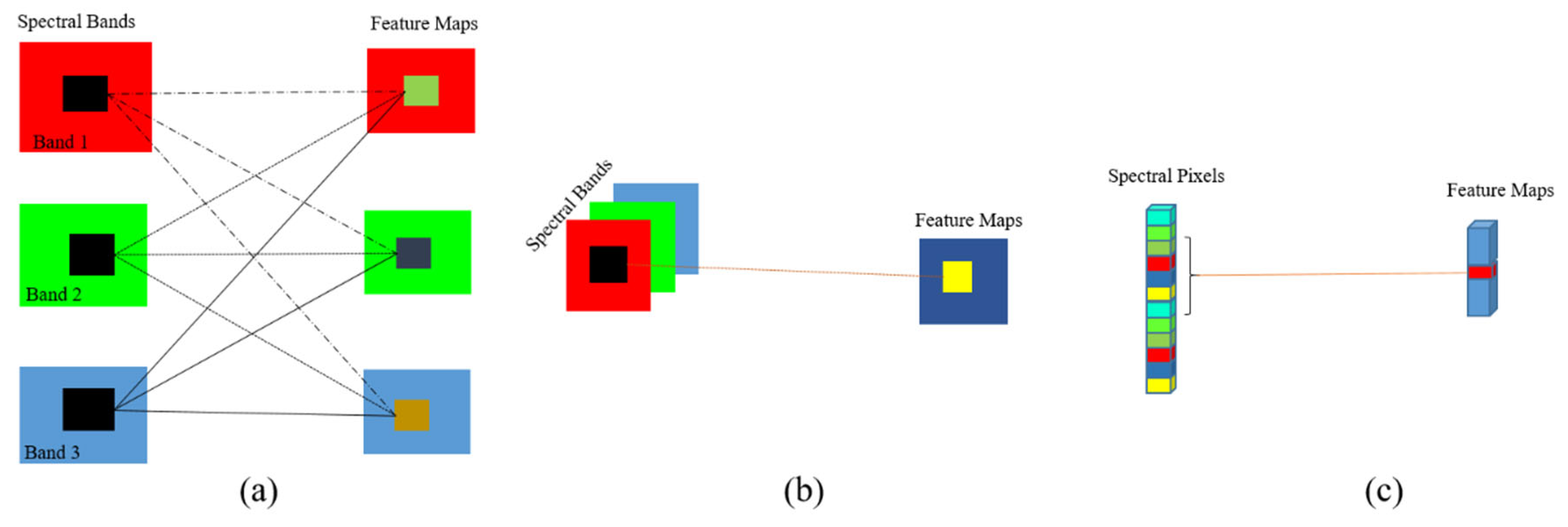
The convolution layer consisted of a set of filters to automatically generate informative features from the raw input data. The kernel of the convolution layer e designed in different dimensional (1D, 2D, and 3D). Figure 4 presents the main difference of kernel convolutions in different dimensions.

The convolution layer uses x as input and provides y in the φth layer using Equation (6).

$$y^{\mathsf{\phi }}=\rho \left(w^{\mathsf{\phi }}{x}^{\mathsf{\phi }-1}\right)+b^{\mathsf{\phi }}$$

(6)

where $\rho$ is the nonlinear activation function, $w$ is the weight in the lth layer, and b is defined as the bias vector of the current layer.

The new output of the ωth feature map in the φth layer ($v_{\mathsf{\phi },\mathsf{\omega }}^{}$) at position (x,y,z) for the 3D-convolution is defined based on Equation (7)

$$v_{\mathsf{\phi },\mathsf{\omega }}^{xyz}=\rho \left(b_{\mathsf{\phi }\mathsf{\omega }}+{{\displaystyle \sum }}_q^{}{{\displaystyle \sum }}_{r=0}^{{\alpha }_{\mathsf{\phi }}-1}{{\displaystyle \sum }}_{s=0}^{{\beta }_{\mathsf{\phi }}-1}{{\displaystyle \sum }}_{t=0}^{{\mathsf{\gamma }}_{\mathsf{\phi }}-1}{W}_{\mathsf{\phi },\mathsf{\omega },q}^{r,s,t}{v}_{\mathsf{\phi }-1,q}^{\left(x+r\right)\left(y+s\right)\left(z+t\right)}\right)$$

(7)

where q is the feature cube connected to the current feature cube in the (φ − 1)th layer; and $\alpha$, $\beta$, and γ are the length, width, and depth of the convolution kernel size, respectively. The output of the 2D convolution layer can be computed using Equation (8).

$$v_{\mathsf{\phi },\mathsf{\omega }}^{xy}=\rho \left(b_{\mathsf{\phi },\mathsf{\omega }}+{{\displaystyle \sum }}_q^{}{{\displaystyle \sum }}_{r=0}^{{\alpha }_{\mathsf{\phi }}-1}{{\displaystyle \sum }}_{s=0}^{{\beta }_{\mathsf{\phi }}-1}{W}_{\mathsf{\phi },\mathsf{\omega },q}^{r,s}{v}_{\mathsf{\phi }-1,q}^{\left(x+r\right)\left(y+s\right)}\right)$$

(8)

The computational in 1D convolution at spatial position x can be expressed based on Equation (9).

$$v_{\mathsf{\phi },\mathsf{\omega }}^x=\rho \left(b_{\mathsf{\phi },\mathsf{\omega }}+{{\displaystyle \sum }}_q^{}{{\displaystyle \sum }}_{t=0}^{{\mathsf{\gamma }}_{\mathsf{\phi }}-1}{W}_{\mathsf{\phi },\mathsf{\omega },q}^r{V}_{\mathsf{\phi }-1,q}^{\left(x+t\right)}\right)$$

(9)

An activation function and a batch normalization function are included in each convolutional layer.

3.4. Accuracy Assessment and Comparison

The results of CD were compared with the reference data (see Section 2) by calculating several accuracy indices, including the OA, F1-Score, Precision, KC, Recall, Miss-Detection (MD), and False Alarm (FA) extracted from a confusion matrix (

Table 1. Confusion matrix.

Confusion Matrix	Predicted
	Change		No-Change
Actual	Change	TP	FN
	No-Change	FP	TN

). The confusion matrix is generated based on four components of True Positive (TP), False Positive (FP), True Negative (TN), and False Negative (FN).

Our proposed method was compared with four other advanced HCD methods to assess its performance. Liu et al. [49] was an unsupervised Multiple HCD framework using the Spectral Unmixing (MSU) method. The second method was introduced by Jafarzadeh and Hasanlou [39], which utilized the Spectral Unmixing (SU) method and similarity measure index. The third HCD method was designed by Hou et al. [50] based on a combination of deep, slow features and differencing (DSFA-Diff) methods. Finally, Du et al. [51] introduced an HCD method based on multiple morphological attributes and spectral angle weighted-based local absolute distance (SALA) methods.

4. Experiments and Results

The weights of the proposed CNN algorithm were initialized using the Glorot normal initializer technique [52]. Moreover, the CNN algorithm was trained with a back-propagation manner and the Adam optimizer. The input patch size was 11 × 11 × 154, and the size of mini-batches was 500. Additionally, the initial learning rate and the number of iterations were set to 10⁻⁴ and 750 epochs, respectively.

The number of sub-regions for the Farmland-1 and Farmland-2 datasets were considered 2 and 7, respectively. The sample data generation results of the proposed method are demonstrated in Figure 5. As can be seen, the generated samples had a high correlation with the reference data.

The results of the statistical accuracy assessment of the sample data generation method for sample regions (Figure 5a,d) are provided in

Table 2. The sample data generation accuracy levels by the proposed hierarchical Otsu thresholding. Level-0 and Level-1 indicate when the original and the proposed hierarchical Otsu thresholding methods were employed.

Dataset	Level	OA	KC	TP	TN	FP	FN
Farmland-1	I	93.97	0.865	4968	2377	386	85
	II	98.51	0.964	4968	2056	21	85
Farmland-2	I	97.08	0.938	4317	7037	309	32
	II	99.53	0.990	3831	7037	19	32

. Based on the results, utilizing the hierarchical Otsu algorithm increased the reliability of the sample data generation. For example, for the Farmland-1 dataset, the OA was 93.97 when the original Otsu method was used (i.e., Level-I). However, it was increased by 4.5% when the hierarchical Otsu thresholding method was employed (i.e., Level-II).

The generated sample data were randomly divided into three groups. Figure 5b,e illustrates the distribution of the reference data, and

Table 3. Numbers of reference samples in the two hyperspectral datasets which were used for HCD.

Case Study	All Sample Data	Training (50%)	Validation (17%)	Testing (33%)
Farmland-1	7130	3566	1212	2352
Farmland-2	10,919	5460	1856	3603

provides the number of the generated samples.

The results of the HCD using the proposed framework and the SU and MSU methods for the Farmland-1 dataset are presented in Figure 6. The results are different, especially in the areas where no changes occurred (i.e., there are no FN pixels). Relatively, more no-change areas were considered as change pixels using the MSU, DSFA-Diff, and SU methods. However, the proposed CD method showed a high performance compared to the reference data (i.e., Figure 6d). Furthermore, there were many FN pixels in the result of the SALA method.

Figure 7 shows the errors using different HCD algorithms for the Farmland-1 dataset. SU, DSFA-Diff, and MSU CD methods had significant amounts of FP and FN pixels (i.e., red and blue colors, respectively). Overall, the proposed HCD method had the least number of errors.

The result of the numerical analysis of the HCD methods for the Farmland-1 dataset is presented in

Table 4. The accuracy of different HCD methods for the Farmland-1 dataset.

Method	DSFA-Diff	SU	MSU	SALA	Propose-Method
OA (%)	86.64	92.50	95.16	94.65	96.33
Precision (%)	73.25	95.37	93.07	86.30	94.35
MD (%)	9.80	16.85	8.40	1.50	6.04
FA (%)	15.0	2.25	3.17	7.10	2.57
F1-Score (%)	80.86	88.83	92.32	92.01	94.15
Recall (%)	90.23	83.14	91.59	98.53	93.95
KC	0.71	0.83	0.89	0.880	0.91

. Our framework had a higher performance than other methods. The OA and KC of the proposed framework were more than 96% and 0.91, respectively. The SU method also had good performance in detecting TP pixels, although it had a limitation in detecting TN pixels.

The result of binary change maps for the Farmland-2 dataset using different HCD methods is also presented in Figure 8. The proposed method provided relatively better performance and lower FA rates.

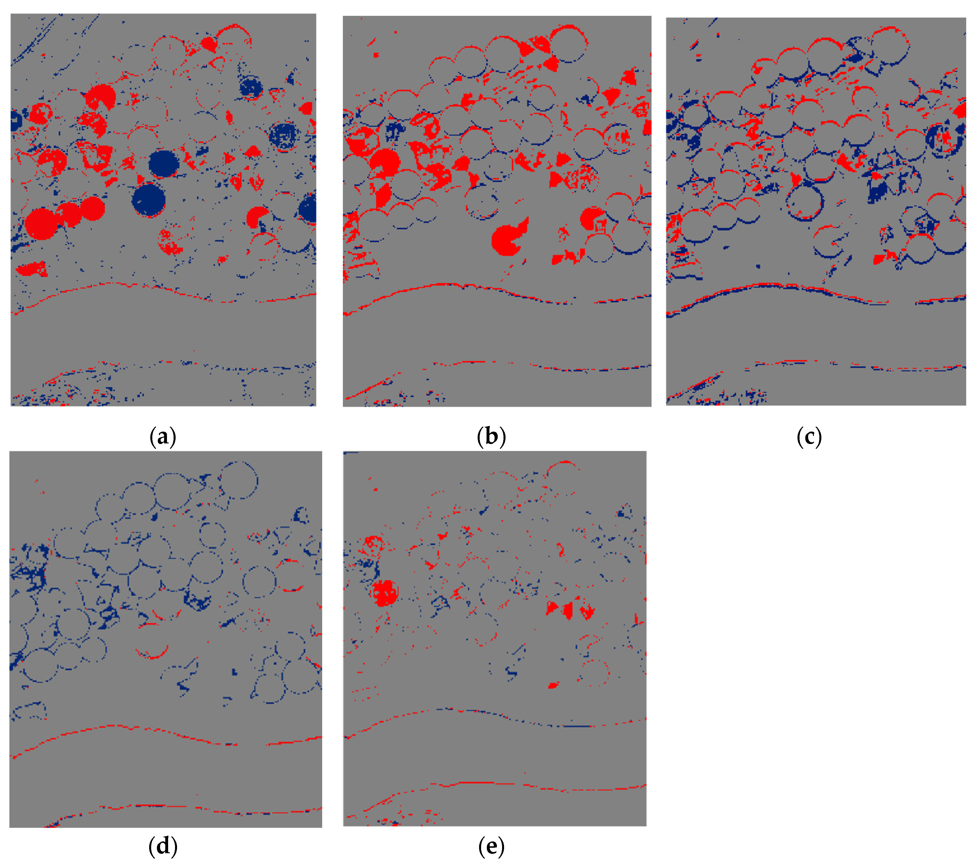
The CD errors using different methods for the Farmland-2 dataset were also evaluated, and the results are demonstrated in Figure 9. It was observed that the SALA and proposed method had lower FP and MD pixels than the other methods. Overall, the proposed method resulted in the lowest FP pixels but more FN pixels than SALA.

The statistical accuracy indices obtained by different HCD methods for the Farmland-2 dataset are also presented in

Table 5. The accuracy of different HCD methods for the Farmland-2 dataset.

Method	DSFA-Diff	SU	MSU	SALA	Propose-Method
OA (%)	88.38	90.06	89.68	95.96	96.86
Precision (%)	72.37	63.10	80.78	85.25	94.62
MD (%)	35.45	9.92	24.55	4.31	11.20
FA (%)	5.87	9.95	5.76	4.02	1.42
F1-Score (%)	68.22	74.21	78.02	90.16	91.72
Recall (%)	64.52	90.08	75.45	95.67	88.99
KC	0.61	0.68	0.72	0.876	0.898

. Based on the results, all HCD algorithms had relatively lower performance than the results obtained for the Farmland-1 dataset. This issue was more severe for the MSU and SU methods in terms of OA, KC, and PCC. For this dataset, the FA and PCC were considerably different compared to the results of the Farmland-1 dataset. Although the SALA method had the lowest MD rate, it had a high FA rate (more than 4%). Generally, the proposed method provided the highest accuracy and lowest error compared to the other four HCD methods.

The ablation analysis in deep learning frameworks measures a network’s performance after removing one or more components to understand how the ablated components contribute to the overall performance. We removed the 1D/2D/3D convolution layers to consider the effects of these layers in our proposed method. In this regard, four scenarios were considered: (S#1) without 1-D convolution layers, (S#2) without 2-D convolution layers, (S#3) without 3-D convolution layers, and (S#4) proposed method with all components. The result of the ablation analysis of the proposed method for the Farmland-2 dataset is presented in

Table 6. The ablation analysis of the proposed HCD method for different scenarios. Scenario 1: without 1-D convolution layers. Scenario 2: without 2-D convolution layers. Scenario 3: without 3-D convolution layers. Scenario 4: the proposed method with all components.

Method	Scenario 1	Scenario 2	Scenario 3	Propose-Method
OA (%)	95.55	95.05	96.18	96.86
Precision (%)	87.98	92.52	93.27	94.62
MD (%)	11.10	18.8	13.50	11.20
FA (%)	2.90	1.60	1.50	1.20
F1-Score (%)	88.45	86.46	89.74	91.72
Recall (%)	88.92	81.16	86.48	88.99
KC	0.857	0.834	0.874	0.898

. The 2D and 3D convolution layers had the highest and lowest impact on the proposed HCD method, respectively.

5. Discussion

Based on the results, hyperspectral imagery is an excellent resource for CD purposes, providing an average OA of more than 90% using different HCD algorithms. The SU method had a low FA (2.25%) rate and a high MD rate (16.85%) for the Farmland-1 dataset. There is, however, a trade-off between detecting change and non-changed classes. For example, the SALA method provided lower MD rates in both datasets but had higher FA rates than the proposed method. Ideally, a method should be able to detect both change and no-change pixels with the lowest error.

The DTW model is a robust predictor and can efficiently predict the change and no-change areas. One of the main limitations of the original DTW predictor is that it takes more time to predict the bi-temporal hyperspectral datasets (about 5 h). However, our proposed method improved the time processing of HCD (less than one hour). Another limitation of the original DTW predictor is that it utilizes only a spectral dataset for HCD. However, in this study, both spatial/spectral features were combined to enhance the results of HCD.

DL methods need a high number of sample datasets, which is usually a challenge for bi-temporal datasets. Additionally, the sample dataset’s quality and quantity are other challenges for the supervised methods. The proposed method in this study did not require setting parameters and collecting user training data. This could significantly reduce the cost and time.

Recently, several HCD methods were proposed to generate sample data using an unsupervised framework [53]. Mainly, these methods generate the sample data with a traditional predictor (i.e., principal component analysis, change vector analysis) and thresholding methods. Although they obtained promising results, the generation of reliable sample data is still challenging. The unreliable sample data result in low accuracies because the supervised classifiers are trained with false sample data. One of the achievements of the proposed method was refining sample data in a hierarchical thresholding method to improve the reliability of sample data. Additionally, utilizing a robust predictor (i.e., DTW algorithm) helped achieve promising results.

Although hyperspectral imagery contains rich spectral information, spatial features should also be included in the HCD process to obtain more accurate results. Most HCD methods have only utilized spectral features, neglecting the importance of spatial features. On the other hand, although there are many methods to extract spatial features, they need to optimize them. Optimizing these features by optimization algorithms is a big challenge and time confusing. This issue can reduce the accuracy of HCD using both traditional and advanced methods. The proposed method could automatically extract the deep features containing spatial and spectral information. In conclusion, the proposed method yielded accurate and reliable results for HCD.

The proposed method contained multi-dimensional convolution layers to improve the results of HCD. Although there are many DL methods based on only 2-D convolution filters, the proposed method used 3D dilated convolution to employ both spatial features and the relationship between spectral bands and, consequently, improved the accuracy of HCD. Additionally, the dilated convolution increased the receptive field without missing information. Furthermore, this research replaced the 2D convolution layer with 1D kernel convolution to decrease the number of parameters of the proposed network. This also decreased the time of the learning process.

The proposed HCD method effectively extracted the changes in an automatic framework. In this study, we focused on binary change detection, though multi-change detection could provide more details of changes. Thus, our future work will be focused on developing a new HCD method for multiple change detection.

6. Conclusions

Developing robust and reliable HCD algorithms is a relatively challenging task due to the specific content of the hyperspectral data, such as a high number of spectral bands and noise conditions. It is also essential to develop an HCD algorithm that can effectively utilize spectral and spatial features within hyperspectral imagery to improve the result of CD. Although DL methods have proved to be efficient for HCD, they require a large number of samples to produce accurate CD results. In this study, a new HCD method based on deep Siamese CNN was proposed for HCD to resolve some of the HCD challenges. The hierarchical Otsu thresholding within the proposed framework improved the performance of the sample generation by producing a high number of reliable sample data. The proposed CNN architecture also improved the HCD by employing spatial and spectral deep features. In addition to comparing the results with the reference data and state-of-the-art CD methods, the proposed method was applied to two bi-temporal hyperspectral datasets. According to the results, hyperspectral imagery has a high potential for CD purposes but requires special techniques to extract change information accurately. Based on visual and statistical accuracy analyses, in comparison with other state-of-the-art HCD methods, the proposed method has the following advantages: (1) it provides a higher accuracy (more than 93%) as well as low MD and FA rates; (2) it is an automatic framework and did not require collecting training data; (3) it is robust to a variety of datasets and land cover classes, (4) it can effectively extract robust deep features using multi-dimensional kernel convolution. All of these advantages illustrate the high potential of the proposed DL framework for different HCD applications.

References

- Song, Y.; Chen, B.; Kwan, M.-P. How does urban expansion impact people’s exposure to green environments? A comparative study of 290 Chinese cities. J. Clean. Prod. 2020, 246, 119018. [Google Scholar] [CrossRef]
- Koko, A.F.; Yue, W.; Abubakar, G.A.; Hamed, R.; Alabsi, A.A.N. Monitoring and Predicting Spatio-Temporal Land Use/Land Cover Changes in Zaria City, Nigeria, through an Integrated Cellular Automata and Markov Chain Model (CA-Markov). Sustainability 2020, 12, 10452. [Google Scholar] [CrossRef]
- Çağlıyan, A.; Dağlı, D. Monitoring Land Use Land Cover Changes and Modelling of Urban Growth Using a Future Land Use Simulation Model (FLUS) in Diyarbakır, Turkey. Sustainability 2022, 14, 9180. [Google Scholar] [CrossRef]
- Kuzevic, S.; Bobikova, D.; Kuzevicova, Z. Land Cover and Vegetation Coverage Changes in the Mining Area—A Case Study from Slovakia. Sustainability 2022, 14, 1180. [Google Scholar] [CrossRef]
- Daba, M.H.; You, S. Quantitatively assessing the future land-use/land-cover changes and their driving factors in the upper stream of the Awash River based on the CA–markov model and their implications for water resources management. Sustainability 2022, 14, 1538. [Google Scholar] [CrossRef]
- Quan, Q.; Gao, S.; Shang, Y.; Wang, B. Assessment of the sustainability of Gymnocypris eckloni habitat under river damming in the source region of the Yellow River. Sci. Total Environ. 2021, 778, 146312. [Google Scholar] [CrossRef]
- Zhang, K.; Wang, S.; Bao, H.; Zhao, X. Characteristics and influencing factors of rainfall-induced landslide and debris flow hazards in Shaanxi Province, China. Nat. Hazards Earth Syst. Sci. 2019, 19, 93–105. [Google Scholar] [CrossRef] [Green Version]
- Luppino, L.T.; Kampffmeyer, M.; Bianchi, F.M.; Moser, G.; Serpico, S.B.; Jenssen, R.; Anfinsen, S.N. Deep image translation with an affinity-based change prior for unsupervised multimodal change detection. IEEE Trans. Geosci. Remote Sens. 2021. [Google Scholar] [CrossRef]
- Wang, S.; Zhang, K.; Chao, L.; Li, D.; Tian, X.; Bao, H.; Chen, G.; Xia, Y. Exploring the utility of radar and satellite-sensed precipitation and their dynamic bias correction for integrated prediction of flood and landslide hazards. J. Hydrol. 2021, 603, 126964. [Google Scholar] [CrossRef]
- Zhao, F.; Song, L.; Peng, Z.; Yang, J.; Luan, G.; Chu, C.; Ding, J.; Feng, S.; Jing, Y.; Xie, Z. Night-time light remote sensing mapping: Construction and analysis of ethnic minority development index. Remote Sens. 2021, 13, 2129. [Google Scholar] [CrossRef]
- Chen, Y.; Bruzzone, L. Self-supervised Change Detection in Multi-view Remote Sensing Images. arXiv 2021, arXiv:2103.05969. [Google Scholar]
- Zhou, H.; Zhang, M.; Hu, X.; Li, K.; Sun, J. A Siamese convolutional neural network with high–low level feature fusion for change detection in remotely sensed images. Remote Sens. Lett. 2021, 12, 387–396. [Google Scholar] [CrossRef]
- Arroyo-Mora, J.P.; Kalacska, M.; Løke, T.; Schläpfer, D.; Coops, N.C.; Lucanus, O.; Leblanc, G. Assessing the impact of illumination on UAV pushbroom hyperspectral imagery collected under various cloud cover conditions. Remote Sens. Environ. 2021, 258, 112396. [Google Scholar] [CrossRef]
- Pechanec, V.; Mráz, A.; Rozkošný, L.; Vyvlečka, P. Usage of Airborne Hyperspectral Imaging Data for Identifying Spatial Variability of Soil Nitrogen Content. ISPRS Int. J. Geo. Inf. 2021, 10, 355. [Google Scholar] [CrossRef]
- Xie, R.; Darvishzadeh, R.; Skidmore, A.K.; Heurich, M.; Holzwarth, S.; Gara, T.W.; Reusen, I. Mapping leaf area index in a mixed temperate forest using Fenix airborne hyperspectral data and Gaussian processes regression. Int. J. Appl. Earth Obs. Geoinf. 2021, 95, 102242. [Google Scholar] [CrossRef]
- Chang, C.-I.; Chen, J. Orthogonal Subspace Projection Using Data Sphering and Low-Rank and Sparse Matrix Decomposition for Hyperspectral Target Detection. IEEE Trans. Geosci. Remote Sens. 2021. [Google Scholar] [CrossRef]
- Meerdink, S.; Bocinsky, J.; Zare, A.; Kroeger, N.; McCurley, C.; Shats, D.; Gader, P. Multitarget Multiple-Instance Learning for Hyperspectral Target Detection. IEEE Trans. Geosci. Remote Sens. 2021. [Google Scholar] [CrossRef]
- Gao, C.; Wu, Y.; Hao, X. Hierarchical Suppression Based Matched Filter for Hyperspertral Imagery Target Detection. Sensors 2021, 21, 144. [Google Scholar] [CrossRef] [PubMed]
- Hasanlou, M.; Seydi, S.T. Hyperspectral change detection: An experimental comparative study. Int. J. Remote Sens. 2018, 39, 7029–7083. [Google Scholar] [CrossRef]
- Ghamisi, P.; Yokoya, N.; Li, J.; Liao, W.; Liu, S.; Plaza, J.; Rasti, B.; Plaza, A. Advances in hyperspectral image and signal processing: A comprehensive overview of the state of the art. IEEE Geosci. Remote Sens. Mag. 2017, 5, 37–78. [Google Scholar] [CrossRef] [Green Version]
- Kim, J.; Lee, M.; Han, H.; Kim, D.; Bae, Y.; Kim, H.S. Case Study: Development of the CNN Model Considering Teleconnection for Spatial Downscaling of Precipitation in a Climate Change Scenario. Sustainability 2022, 14, 4719. [Google Scholar] [CrossRef]
- Tsokov, S.; Lazarova, M.; Aleksieva-Petrova, A. A Hybrid Spatiotemporal Deep Model Based on CNN and LSTM for Air Pollution Prediction. Sustainability 2022, 14, 5104. [Google Scholar] [CrossRef]
- Liu, F.; Xu, H.; Qi, M.; Liu, D.; Wang, J.; Kong, J. Depth-Wise Separable Convolution Attention Module for Garbage Image Classification. Sustainability 2022, 14, 3099. [Google Scholar] [CrossRef]
- Li, S.; Liu, C.H.; Lin, Q.; Wen, Q.; Su, L.; Huang, G.; Ding, Z. Deep residual correction network for partial domain adaptation. IEEE Trans. Pattern Anal. Mach. Intell. 2020, 43, 2329–2344. [Google Scholar] [CrossRef] [Green Version]
- Zhang, Q.; Ge, L.; Hensley, S.; Metternicht, G.I.; Liu, C.; Zhang, R. PolGAN: A deep-learning-based unsupervised forest height estimation based on the synergy of PolInSAR and LiDAR data. ISPRS J. Photogramm. Remote Sens. 2022, 186, 123–139. [Google Scholar] [CrossRef]
- Sefrin, O.; Riese, F.M.; Keller, S. Deep Learning for Land Cover Change Detection. Remote Sens. 2021, 13, 78. [Google Scholar] [CrossRef]
- Chen, H.; Zhang, K.; Xiao, W.; Sheng, Y.; Cheng, L.; Zhou, W.; Wang, P.; Su, D.; Ye, L.; Zhang, S. Building change detection in very high-resolution remote sensing image based on pseudo-orthorectification. Int. J. Remote Sens. 2021, 42, 2686–2705. [Google Scholar] [CrossRef]
- Wang, C.; Wang, X. Building change detection from multi-source remote sensing images based on multi-feature fusion and extreme learning machine. Int. J. Remote Sens. 2021, 42, 2246–2257. [Google Scholar] [CrossRef]
- Seydi, S.; Hasanlou, M. Binary Hyperspectral Change Detection Based on 3d Convolution Deep Learning. Int. Arch. Photogramm. Remote Sens. Spat. Inf. Sci. 2020, 43, 1629–1633. [Google Scholar] [CrossRef]
- Huang, F.; Yu, Y.; Feng, T. Hyperspectral remote sensing image change detection based on tensor and deep learning. J. Vis. Commun. Image Represent. 2019, 58, 233–244. [Google Scholar] [CrossRef]
- Wang, L.; Zhang, J.; Liu, P.; Choo, K.-K.R.; Huang, F. Spectral–spatial multi-feature-based deep learning for hyperspectral remote sensing image classification. Soft Comput. 2017, 21, 213–221. [Google Scholar] [CrossRef]
- Ball, J.E.; Anderson, D.T.; Chan Sr, C.S. Comprehensive survey of deep learning in remote sensing: Theories, tools, and challenges for the community. J. Appl. Remote Sens. 2017, 11, 042609. [Google Scholar] [CrossRef] [Green Version]
- Guo, Q.; Zhang, J.; Zhong, C.; Zhang, Y. Change detection for hyperspectral images via convolutional sparse analysis and temporal spectral unmixing. IEEE J. Sel. Top. Appl. Earth Obs. Remote Sens. 2021, 14, 4417–4426. [Google Scholar] [CrossRef]
- Wang, L.; Wang, L.; Wang, Q.; Atkinson, P.M. SSA-SiamNet: Spectral–spatial-wise attention-based Siamese network for hyperspectral image change detection. IEEE Trans. Geosci. Remote Sens. 2021, 60, 1–18. [Google Scholar] [CrossRef]
- Seydi, S.T.; Hasanlou, M. A new land-cover match-based change detection for hyperspectral imagery. Eur. J. Remote Sens. 2017, 50, 517–533. [Google Scholar] [CrossRef]
- Tong, X.; Pan, H.; Liu, S.; Li, B.; Luo, X.; Xie, H.; Xu, X. A novel approach for hyperspectral change detection based on uncertain area analysis and improved transfer learning. IEEE J. Sel. Top. Appl. Earth Obs. Remote Sens. 2020, 13, 2056–2069. [Google Scholar] [CrossRef]
- Liu, L.; Hong, D.; Ni, L.; Gao, L. Multilayer Cascade Screening Strategy for Semi-Supervised Change Detection in Hyperspectral Images. IEEE J. Sel. Top. Appl. Earth Obs. Remote Sens. 2022, 15, 1926–1940. [Google Scholar] [CrossRef]
- Zhan, T.; Song, B.; Sun, L.; Jia, X.; Wan, M.; Yang, G.; Wu, Z. TDSSC: A Three Directions Spectral-Spatial Convolution Neural Networks for Hyperspectral Image Change Detection. IEEE J. Sel. Top. Appl. Earth Obs. Remote Sens. 2020. [Google Scholar] [CrossRef]
- Jafarzadeh, H.; Hasanlou, M. An unsupervised binary and multiple change detection approach for hyperspectral imagery based on spectral unmixing. IEEE J. Sel. Top. Appl. Earth Obs. Remote Sens. 2019, 12, 4888–4906. [Google Scholar] [CrossRef]
- López-Fandiño, J.; Heras, D.B.; Argüello, F.; Dalla Mura, M. GPU framework for change detection in multitemporal hyperspectral images. Int. J. Parallel Program. 2019, 47, 272–292. [Google Scholar] [CrossRef]
- Appice, A.; Di Mauro, N.; Lomuscio, F.; Malerba, D. Empowering change vector analysis with autoencoding in bi-temporal hyperspectral images. In Proceedings of the CEUR Workshop Proceedings, Würzburg, Germany, 20 September 2019. [Google Scholar]
- Song, A.; Kim, Y. Transfer Change Rules from Recurrent Fully Convolutional Networks for Hyperspectral Unmanned Aerial Vehicle Images without Ground Truth Data. Remote Sens. 2020, 12, 1099. [Google Scholar] [CrossRef]
- Seydi, S.T.; Hasanlou, M.; Amani, M. A new end-to-end multi-dimensional CNN framework for land cover/land use change detection in multi-source remote sensing datasets. Remote Sens. 2020, 12, 2010. [Google Scholar] [CrossRef]
- Han, T.; Peng, Q.; Zhu, Z.; Shen, Y.; Huang, H.; Abid, N.N. A pattern representation of stock time series based on DTW. Phys. A Stat. Mech. Appl. 2020, 550, 124161. [Google Scholar] [CrossRef]
- Csillik, O.; Belgiu, M.; Asner, G.P.; Kelly, M. Object-based time-constrained dynamic time warping classification of crops using Sentinel-2. Remote Sens. 2019, 11, 1257. [Google Scholar] [CrossRef] [Green Version]
- Kurita, T.; Otsu, N.; Abdelmalek, N. Maximum likelihood thresholding based on population mixture models. Pattern Recognit. 1992, 25, 1231–1240. [Google Scholar] [CrossRef]
- Goh, T.Y.; Basah, S.N.; Yazid, H.; Safar, M.J.A.; Saad, F.S.A. Performance analysis of image thresholding: Otsu technique. Measurement 2018, 114, 298–307. [Google Scholar] [CrossRef]
- Fang, B.; Li, Y.; Zhang, H.; Chan, J.C.-W. Collaborative learning of lightweight convolutional neural network and deep clustering for hyperspectral image semi-supervised classification with limited training samples. ISPRS J. Photogramm. Remote Sens. 2020, 161, 164–178. [Google Scholar] [CrossRef]
- Liu, S.; Bruzzone, L.; Bovolo, F.; Du, P. Unsupervised multitemporal spectral unmixing for detecting multiple changes in hyperspectral images. IEEE Trans. Geosci. Remote Sens. 2016, 54, 2733–2748. [Google Scholar] [CrossRef]
- Hou, Z.; Li, W.; Li, L.; Tao, R.; Du, Q. Hyperspectral change detection based on multiple morphological profiles. IEEE Trans. Geosci. Remote Sens. 2021, 60, 1–12. [Google Scholar] [CrossRef]
- Du, B.; Ru, L.; Wu, C.; Zhang, L. Unsupervised deep slow feature analysis for change detection in multi-temporal remote sensing images. IEEE Trans. Geosci. Remote Sens. 2019, 57, 9976–9992. [Google Scholar] [CrossRef] [Green Version]
- Glorot, X.; Bengio, Y. Understanding the difficulty of training deep feedforward neural networks. In Proceedings of the Thirteenth International Conference on Artificial Intelligence and Statistics, Sardinia, Italy, 13–15 May 2010; pp. 249–256. [Google Scholar]
- Song, A.; Choi, J.; Han, Y.; Kim, Y. Change detection in hyperspectral images using recurrent 3D fully convolutional networks. Remote Sens. 2018, 10, 1827. [Google Scholar] [CrossRef]
Figure 1.
(a,b) False-color composites of the hyperspectral dataset captured in 2006 and 2007 from the Farmland-1 study area. (c) The binary reference data was generated for the Farmland-1 dataset. (d,e) False-color composites of the hyperspectral dataset were captured in 2004 and 2007 from the Farmland-2 study area. (f) The binary reference data was generated for the Farmland-2 dataset.
Figure 2.
Overview of the proposed framework for HCD.
Figure 3.
The architecture of the proposed deep Siamese CNN for HCD applications. Feature map size is indicated by the numbers.
Figure 4.
Comparison of kernel convolutions. (a) 1-D, (b) 2-D, and (c) 3-D.
Figure 5.
The result of sample data generation for (a–c) Farmland-1 and (d–f) Farmland-2 datasets. White and gray colors demonstrate the TP and TN pixels, respectively.
Figure 6.
The results of binary HCD for the Farmland-1 dataset using (a) DSFA-Diff, (b) SU, (c) MSU, (d) SALA, and (e) proposed methods. (f) Binary reference data. White and black colors demonstrate the TP and TN pixels, respectively.
Figure 7.
The CD errors of (a) DSFA-Diff, (b) SU, (c) MSU, (d) SALA, and (e) proposed for the Farmland-1 datasets. Gray, red, and blue colors demonstrate TP/TN, FN, and FP pixels, respectively.
Figure 8.
The results of binary HCD for the Farmland-2 dataset using (a) DSFA-Diff, (b) SU, (c) MSU, (d) SALA, and (e) proposed methods. (f) Binary reference data. White and black colors indicate the TP and TN pixels, respectively.
Figure 9.
The CD errors of the (a) DSFA-Diff, (b) SU, (c) MSU, (d) SALA, and (e) proposed methods for the Farmland-2 dataset. Gray, red, and blue colors indicate the TP/TN, FN, and FP pixels, respectively.