
A Holistic Review of GM/IM Selection Methods from a Structural Performance-Based Perspective

Department of Civil and Environmental Engineering, Utah State University, Logan, UT 84322, USA
Sustainability 2022, 14(20), 12994; https://0-doi-org.brum.beds.ac.uk/10.3390/su142012994
Submission received: 16 September 2022
/
Revised: 9 October 2022
/
Accepted: 9 October 2022
/
Published: 11 October 2022
(This article belongs to the Special Issue Seismic Retrofit and Rehabilitation Methods for Resilient and Sustainable Structures)
Abstract
:Current fully probabilistic approaches to performance-based earthquake engineering describe structures’ behavior under a wide range of seismic hazard levels. These approaches require a detailed representation of ground motion (GM) uncertainty at all considered hazard levels, yet different GM selection methods lead to different estimations of structural performance. This paper presents a holistic review of the current practices in GM representation and selection for structural demand analysis through a performance-based lens. The multidisciplinary nature of GM selection, ranging from earth science to engineering seismology and statistics, has created a preponderance of literature to find the best practice for probabilistic assessment of structures in terms of computational efficiency and statistical accuracy. Many of these studies focus individually on GM selection or structural analysis, and the relatively scarce review papers either focus on code-based GM selection or do not specifically address risk-based evaluations by overlooking the interaction between GM selection and structural analysis. This paper aims to aid researchers in selecting appropriate GMs as part of a statistically valid and robust probabilistic demand analysis without performing an exhaustive literature review. Discussion on the available computational tools and their trade-offs for risk-based assessment of single structures is provided. While the problem-specific nature of GM selection means that no pre-selected set of GM/IM is applicable to all cases, the comprehensive narrative of this paper is expected to aid analysts in reaching a more informed decision.
1. Introduction
In the last decade, performance-based earthquake engineering (PBEE) introduced a paradigm shift from a prescriptive approach, which only accounts for implicit life safety objectives through ductility and strength requirements, to one that directly quantifies performance under different levels of hazard intensities [1,2,3]. Bertero and Bertero picture PBEE as a framework that monitors both structural and non-structural components at the given seismic excitation levels to ensure they are not damaged beyond pre-specified levels with a certain reliability [4]. Hence, the wide scope of PBEE requires that all important sources of uncertainties be included to accurately capture the structure’s reliability [5]. While PBEE is usually represented as a series of analyses linked by generic “pinch-point variables”, the actual implementation of the approach is significantly more complex, as shown in Figure 1.
The first two steps of PBEE, hazard analysis and structural analysis, comprise probabilistic seismic demand analysis (PSDA), which constructs a probabilistic model of structural response conditioned on the seismic hazard level. Uncertainties in PSDA are attributed to uncertainties in ground motions (GM) and structural seismic demand. Uncertainty in GM stems from a seismic source (occurrence of an event, magnitude, distance, epicenter, and rupture surface), path, and site. Uncertainty in demand depends on ground motion uncertainty, but additionally accounts for structural modeling uncertainty (e.g., elements types that are used to represent actual structure) and structure’s dynamic characteristics (e.g., damping, reactive mass, and force–deformation behavior) [6]. The incorporation of uncertainties in PSDA requires performing a large number of structural analyses, commonly through time-domain analysis, where PSDA accuracy largely depends on the degree to which the GMs represent the true seismic hazard.
The current PBEE literature addresses GM selection by (a) finding the most appropriate proxy for GM uncertainty, frequently an Intensity Measure (IM); and (b) matching the selected proxy to the site hazard. While it is convenient to treat these two steps independently for cases where the IM precisely and accurately describes structure’s response (i.e., IM is a perfect proxy) at all considered hazard levels, recent studies demonstrate that an IM’s ability to meet this requirement also depends on the selected GM set [7,8]. Therefore, this paper will argue that a holistic IM/GM approach is needed.
While a large body of research addresses GM selection, there are three practical obstacles to finding the most relevant information when performing PSDA:
- GM treatments are developed separately for numerous applications, leading to a perplexing literature. For example, most building codes-based methods use the average expected seismic loads and minimize the variability between GMs by scaling them to a predefined design spectrum. In contrast, PBEE preserves the variability between the selected GMs to estimate the structural response distribution parameters [9,10,11]. It can be expected that applying these GM methods out of context will lead to inaccurate performance estimates.
- Even for the same application, the scope and trade-offs between different GM selection methods are unclear or scattered among different references. Various GM uncertainty proxies and matching methods are presented, and it is believed that if best practices are followed, all appropriate choices will yield similar results. However, recent studies [12,13,14] show that the analyst’s choices will lead to significantly different estimations of performance.
- The interaction of GM selection and structural analysis procedure is understudied because GM suites and structural models are generally developed by two different parties. However, high-fidelity models used in recent studies challenge the GM selection methods that are commonly proposed based on simplified models [15,16]. The structure-specific nature of GM/IM selection suggests that a holistic approach is needed to consider structural analysis and modeling in conjunction with IM and GM selection methods.
The primary goal of this paper is to facilitate an informed selection of appropriate GMs to support the PSDA of individual structures. In this regard, a comprehensive review is presented to discuss the available computational methods, their trade-offs, and their effect on PSDA. This review aims to tackle the identified gaps by (i) focusing on information only pertaining to estimating PSDA based on the widely accepted terminology and approaches, (ii) providing complementary perspectives of proposed methods, and when applicable, and (iii) analyzing topics relevant to a structural analysis perspective, such as the bias due to scaling and the required number of records.
The materials covered in this paper are scattered in different sources and, to the best knowledge of the author, a single review paper does not exist that shares the same scope and objective. Therefore, this paper can be considered as an overview of all interconnected topics related to PSDA and is targeted at users with limited exposure to PBEE methodology. Using this review as a first step can save readers time to re-direct effort at the GM selection aspects that are more important for their study. In this regard, the structure of this review paper is organized pragmatically to address the role of GM uncertainties for estimation of structural response (in comparison to other sources of uncertainty), to select appropriate proxies to represent GM uncertainty, and to match those proxies to site hazard through GM selection. Section 2 provides a brief review of PBEE, focusing on the role of GM uncertainty. Section 3 discusses GM uncertainty representation through IM selection, followed by a more detailed discussion of two primary approaches of GM selection methods in Section 4.
2. PBEE Framework
Although the initial idea of probabilistic treatment of structural response was established in the 1960s [17], early efforts in “modern” PBEE are commonly traced to the Vision 2000 report of the Structural Engineers Association of California (SEAOC) in 1995. This pioneering report (and following guidelines, such as FEMA 273, FEMA 274, and FEMA 356) redefines a performance objective as the expected damage level under a given earthquake shaking level, where damage is measured in terms of local criteria imposed at component-level deformation and strength [18,19,20]. The Pacific Earthquake Engineering Research (PEER) Center refined and extended the scope of the first-generation of performance-based guidelines in their fully probabilistic framework. As shown in Figure 1, the PEER-PBEE framework (herein referred to as PBEE) consists of four distinct stages: hazard analysis, structural analysis, damage analysis, and loss analysis. The framework relies on the total probability theorem to propagate uncertainties (i.e., measuring the impact of input randomness on response randomness) from each stage using intermediate random variables (i.e., pinch point variables). It implicitly assumes that the result of each stage is solely dependent on the immediate predecessor stage, commonly referred to as the Markovian assumption. In this manner, the mean annual frequency of performance metrics expressed as decision variables (DV) (e.g., financial or human loss, downtime) can be expanded using the “pinch points” of each stage, which are ground motion’s intensity measures (IM), structure’s engineering demand parameters (EDP), and component’s damage state (DS), respectively [21]. A series of conditional distributions are convolved as follows [22]:
where G(X|Y) is the conditional complementary cumulative distribution of X given Y, and λ is the mean annual frequency of exceeding a threshold for a given decision variable. PSDA performs integration on the last two right-sided terms of the integrand in Equation (1) and estimates the mean annual frequency of exceeding a particular EDP level as follows:
Figure 2 compares the estimation of using two structural analysis methods. While is theoretically unique for each structure, depends on the conditioning IM, as EDP can exceed a given level, edp, at different IM levels (i.e., if a vertical line is positioned at IM-EDP plots in Figure 2, it crosses different IM values) [23]. In addition, for the same GM suite consisting of n records, the two represented methods treat GMs differently, which results in different EDP-IM data. Hence, estimations from these methods are likely to be different at certain IM levels. These observations illustrate the IM/GM selection salience in PSDA applications. Structural analysis methods are further discussed in Section 2.3.
2.1. Treatment of Uncertainty in PBEE
At the broadest level, uncertainty is induced by either lack of knowledge (i.e., epistemic) or inherent randomness/variability (i.e., aleatory). While this distinction is not always apparent, the effects of these two uncertainty types on the estimated performance are different. In practical terms, aleatory uncertainties are related to the point estimates (e.g., mean) of performance probabilities, whereas the epistemic uncertainties determine the confidence in the estimated probabilities (e.g., confidence intervals) [24]. The current PBEE practice follows a parametric approach, where a probability distribution (i.e., probabilistic model) is assigned to the aleatory uncertainty, and the distribution’s parameters are estimated from the numerical models and/or available data using the method of moments or maximum likelihood estimation. If uncertainty is dominated by a single source, a probabilistic distribution for that source can be assumed and approximate measures can be used for other sources of uncertainty [25]; this approximation is largely followed by the current practice of the PBEE community, as will be discussed in Section 2.2. The model’s epistemic uncertainties are addressed either using reliability methods or sampling-based approaches.
Uncertainty can also be modeled using probabilistic methods such as Bayesian statistics [26,27], which combines experts’ judgment and scarce data, or non-probabilistic methods such as the Dempster–Shafer theory [28] of evidence or fuzzy sets [29]. The choice is mostly driven by the availability of data, hence when sufficient data are available, as assumed to be the case in PSDA, statistical methods based on numerical models or data are more favorable [30].
2.2. The Role of GM Uncertainty in PBEE
It is commonly assumed that GM variability governs all other sources of uncertainty in PSDA, which has resulted in the disproportionately larger body of research of GM uncertainty with respect to all other sources of uncertainty in PBEE. Wen argues that since the variability (in terms of coefficient of variation) of ground motion is generally about twice that of the capacity, their effects can be decoupled by using a mean value for capacity and a full probabilistic model for ground motion variability [31]. Kwon and Elnashai investigated the effect of material and ground motion variability in PSDA of an ordinary RC frame and conclude that GM variability has the most significant role, whereas material properties play a smaller role only at higher shaking intensity [32]. Porter et al. investigated a high-rise non-ductile RC frame and compared the effect of uncertainties associated with the ground motion, mass, damping, component force–deformation relationship, component fragility, contractor cost, and profit on the repair cost, and find that uncertainties in ground motion are one of the two main contributors [33]. Celik and Ellingwood studied three non-ductile RC frames and concluded that since the median fragilities (considering only GM uncertainties) were enclosed by the 95% confidence bounds of fragilities considering both modeling and GM uncertainties, the GMs’ uncertainty governed the overall response [34].
Despite the vast body of research favoring GM uncertainty as the main contributor, some recent studies suggest that other sources of uncertainty (such as modeling uncertainties) might be significant, as they affect both the median and dispersion of estimated response. Celarec and Dolĕk investigated the effect of concrete strength, steel strength, mass and beams and columns yield, and ultimate rotation of three non-ductile and ductile RC structures, and found that the important parameters vary with structures. For example, the ductile building’s response was controlled by the ultimate rotation of beams, whereas the non-ductile building was controlled by the ultimate rotation of columns [35]. Jalayer et al. considered modeling uncertainties by assuming a prior distribution of design parameters and then used a Bayesian updating approach to derive the posterior distribution of modeling parameters and structural performance. The authors demonstrated that modeling uncertainties increase both demand/capacity ratio median and standard deviation [36]. Gokkaya et al. showed that if a GM set is selected based on the site’s seismicity, the impacts of modeling uncertainties depend on the performance metric and demand parameter of interest. While modeling uncertainty could significantly increase the mean annual frequency of collapse, it has a limited effect on median drifts below 7% [13]. A recent experimental study by Deng et al. on nonlinear oscillators under seven GMs showed that the uncertainty contributions of structural and GMs change with the intensity level, and that GM uncertainty is not always the governing source [14]. While the limited number of GMs does not allow to establish a general trend, it casts additional doubts on the assumption of the higher significance of GM uncertainty. Tarbali et al. investigated the effect of epistemic uncertainties in GM selection and concluded that while it has a negligible effect at low demand, its contribution in regard to other sources of epistemic uncertainties (such as hazard analysis and site response) increases for near-collapse states [37]. Bradley pointed out that the studies emphasizing GM uncertainties are not consistent in their treatment of the uncertainties: GM uncertainty is overestimated due to the relaxed selection of a large number of GMs, whereas modeling uncertainties are underrepresented due to the inclusion of only low-level uncertainties [38].
To summarize, while there is a consensus on the role of GM uncertainty, other sources of uncertainty, such as modeling uncertainty, can be substantial, particularly at near-collapse limit states.
2.3. Structural Analysis Procedures
Three popular procedures are available to estimate using nonlinear dynamic analysis: cloud analysis [39], multiple stripe analysis (MSA) [40], and incremental dynamic analysis (IDA) [41]. IDA successively scales the selected GMs to increasing amplitude using the same GM suite [42,43], whereas MSA uses different GMs at different hazard levels. In cloud analysis, structures are subjected to a large number of records, and the relationship between IM and EDP (i.e., a cloud of IM-EDP data points) is modeled using a regression model [44]. Here, GMs are considered more as loading protocols to assess a structure’s behavior under a wide range of shaking levels. Although cloud analysis is inherently simple and reduces the number of required analyses significantly as opposed to IDA or MSA, it is constrained by the limitations of its underlying regression assumptions (e.g., homoscedasticity of residuals) and high sensitivity to GM selection [45]. It should be noted that some recent studies aim to improve the current analyses methods to use fewer ground motions, for example, through constraining the number of stripes in MSA [46].
Comparison of different analysis procedures has not received wide attention, and only a few studies assessed the results obtained from different procedures using realistic structural models. Bai et al. compared IDA and cloud analysis for 2- and 5-story RC office buildings and showed that the methods provide a consistent prediction of elastic slope and yield onset [47]. It should be noted that their IDA is constructed using a single record with scaling factors from 1 to 10, whereas the GM suite for cloud analysis consists of 160 unscaled records. Therefore, care should be given not to extend their conclusion to the consistency of the results from the two methods, as the IDA procedure was extremely limited. Nassirpour et al. compared cloud and IDA for 2- and 4-story steel frames and showed that while the results are mostly consistent for lower damage levels, they show significantly different values at larger damage states related to higher shaking intensities [48]. It should be noted this study uses 150 unscaled for cloud and scaled FEMA P695 records from 0.05 g to 2.6 g for IDA. Banerjee et al. showed that for a 3-story RC frame, obtained from MSA and IDA are very different [49]. Two different GM suites were used, which comprised 11 and 43 records for IDA and MSA, respectively.
The reviewed studies used different GMs for each method, preventing the impact of GM analysis to be isolated from GM selection. In this regard, Mackie and Stojadinović compared a more consistent IDA and cloud analysis (GMs were selected based on magnitude-distance bins and soil type for cloud analysis with a subset from the same GMS used for IDA) for a highway overpass bridge and concluded they yield interchangeable PSDA results [50]. However, more studies with consistent GM selection are needed to assess the role of different GM analysis methods.
As a final remark, the method to estimate varies with the analysis procedure due to differing IM-EDP data collection [51]. For example, while most IDA studies use the method of moments [42] to estimate the mean and standard deviation of response conditional distribution, MSA uses maximum likelihood estimation due to the discontinuity of data (i.e., some GMs might not show collapse and a strictly increasing relationship between IM and collapse is not observed) [51]. This non-uniformity of estimated is the main argument in support of interaction between structural analysis and GM selection method and should be kept in mind in PSDA applications.
3. Representing GM Uncertainties
GM uncertainty is commonly described using either stochastic GM models or intensity measures (IM) [40]. A stochastic GM model modifies a white noise sequence based on expected spectral and temporal ground motion features. The modification is made either by using the fault physics to describe the GM radiation spectrum through the product of source, path, and site functions (source-based models), or by fitting a pre-selected mathematical model to a suite of recorded GMs (i.e., site-based models) [52]. As stochastic GMs are uncommon in conventional PBEE (except for sites with infrequent seismic activities), this review only focuses on IM selection. Following a primer on IM definition and limitation, the remaining sections discuss IM selection criteria, different types (single and vector) of IMs, and proposed optimal IMs.
3.1. Intensity Measures (IMs)
Intensity measures explicitly describe the salient features of GMs. The term “explicit” is used to distinguish IMs from other measures that are not directly related to the severity of GM records; these non-explicit measures are commonly referred to as causal parameters [53]. The reason behind the IM approach’s ubiquity in PBEE is that it facilitates an uncoupled framework, where structural and seismic hazard analyses are treated separately [54]. An earthquake has different features (such as magnitude, energy content, and duration), and it is the analyst’s responsibility to determine which features are important for a given structure, and hence should be captured using an IM. However, such expertise often is not available to the structural engineer performing PSDA.
The task of choosing the right IM is seldom straightforward, and the literature is frequently conflicting. A prominent example of literature confliction is the GM duration. Early studies measured the correlation between duration and peak displacement demands and suggested that duration is not important [55], whereas successor studies found a significant association between duration and cumulative response measures [56]. Raghunandan and Liel performed multivariate regression on the collapse of a 4-story RC building and noted that when GMs with the same inelastic spectral displacement intensities are compared, the ones with the longer duration caused collapse at lower IM levels. However, the extent of the duration effect depends on the other considered IMs and the structure’s ductility [57]. Chandramohan et al. suggested that duration is more important for near-collapse limit states at sites where large magnitude interface earthquakes have the largest contribution [58]. These examples emphasize that the selected IMs are largely problem-specific and structural and seismological issues affect the choice of IM, hence the scope and limitations of each IM should be carefully understood. In this regard, after an extensive investigation of IM selection criteria and types in the following sections, the scope of several different proposed IMs is summarized as a first step for IM selection in future studies.
3.2. IM Selection Criteria
As IMs are the medium by which structural response is related to a site’s seismic hazard, the accuracy of PBEE’s convolution relies on the appropriateness of the adopted IM. As shown in Table 1, the appropriateness of an IM can be assessed through different criteria such as “efficiency” [59], “sufficiency” [59], “practicality” [59], “hazard computability” [60], “scaling robustness” [61], and “proficiency” [62]. An efficient (precise) IM reduces the dispersion of the estimated seismic response conditioned on the IM (i.e., EDP|IM), which subsequently reduces the number of required analyses. On the other hand, sufficiency (accuracy) determines whether the structural response is independent of all other site hazard characteristics that are not captured by the adopted IM, that is, seismological parameters such as magnitude and distance [59]. Hazard computability examines the effort required to calculate the IM hazard curve, and frequently encapsulates whether or not the IM is a direct output of conventional hazard analysis [60]. Scaling robustness requires scaled records to yield an unbiased response estimation, and is assessed by regressing responses subjected to the GMs with the same IM values to scale factors [61]. Practicality refers to the dependence of the response to the IM, and is measured by the slope of EDP-IM regression [62] where a weak slope shows lower practicality. Finally, proficiency represents the combined effect of practicality and efficiency [62]. Khosravikia and Clayton argued that using practicality to compare different IMs with different ranges is not fair due to their impact on regression slope. In addition, they discussed that efficiency cannot capture the correlation of PSDA and time-history analysis and, while adequate for a single EDP, are not suitable to compare different types of structures or structural responses. Instead, they suggested modifications to the original definitions to extend their scope [63].
Compared to other criteria, efficiency and sufficiency have gained more attention, as they are deemed necessary conditions for a valid combination of the results of hazard and structural analyses [64]. Some authors even argue that a sufficient IM might render a careful GM selection unnecessary [60]. Interestingly, the structural engineering literature favors the IM’s association with the parameters of EDP distribution over considering them as direct estimators of site seismic hazard. In this regard, the notion of estimator’s efficiency is borrowed from statistical inference, and efficiency is measured by comparing the variance of EDPs’ residuals regressed on IM (i.e., ). However, establishing a mathematical notion for sufficiency is shown not to be as straightforward. Luco and Cornell [59] used the p-value test to examine whether the is dependent on any other seismological parameter, namely magnitude and distance. A p-value larger than a significant level of interest (commonly taken as 0.05) shows that residuals cannot be described by the considered seismological parameters, hence the IM is sufficient in regard to that parameter. While this procedure is straightforward, it cannot measure the extent of the sufficiency of different IMs. For a given EDP and ground motion suite, several IMs can have p-values that are higher than the significance level and are identified as sufficient (as shown by [65], among others). In addition, while a small p-value can be used to argue that a statistically significant relationship between seismological parameters and exists, it is questionable to use a large p-value to support that such a relationship does not exist.
Following the literature on information theory, Jalayer et al. defined sufficiency as reducing and preserving the information in the GM records to estimate EDP as follows [66]:
where is the acceleration history of a given record. Since sufficiency, in an absolute sense, requires that all the different levels of the IM be independent of any given seismological features, a relative measure can alleviate the computational expense [66]. Jalayer et al. proposed a relative sufficiency measure based on average information gain that one IM can provide over another one, as follows [66]:
To obtain , one must calculate , which represents all possible earthquakes at the site. The exact approach then extends the above integration to seismological parameters of interest (e.g., M and R) and uses hazard deaggregation to compute the joint probability of those seismological parameters (e.g., p(M,R)) in combination with a stochastic ground motion model to obtain . To avoid the need for hazard deaggregration and joint treatment of causal parameter variability, Jalayer et al. approximated Equation (4) for a selected suite of GMs as follows:
It should be noted that the selected suite might not represent the site characteristics accurately, and different conclusions might be drawn from the application of Equation (4) and Equation (5) [66]. Nevertheless, some studies have used the approximate approach for preliminary ranking of sufficiency of different IMs for medium-rise RC [67] or high-rise core-tube buildings [68].
Recently, Dhulipala et al. have shown that is a measure of efficiency (and not sufficiency), if the logarithms of EDP and IM are used in Equation (5) and subsequently, the sum of squares of errors is minimized [7]. Instead, the authors quantified sufficiency by measuring the deviation of the conditional distribution of IMi on EDP with and without considering the jth seismological parameters. The information gain due to the inclusion of jth parameter is summed to calculate the total information gain for IMi, TIGi, as follows:
where and represent the conditional distribution of the ith IM given EDP with and without considering the jth seismological parameter, respectively. The authors studied a 4-story steel frame and showed that sufficiency (using Equation (6)) and efficiency have a bivariate normal distribution with a low correlation value of 0.3, and therefore a strong efficiency does not enforce a similar sufficiency. In addition, they found sufficiency to depend on ground motion selection.
To conclude, since it is practically infeasible to obtain an IM that is sufficient for different levels of site’s hazard and structure’s response, a practical approach is to combine relatively efficient IMs with carefully selected (e.g., hazard-consistent) GMs to introduce the least bias in risk estimation.
3.3. Scalar and Vector IMs
IMs can be classified as scalar and vector IMs, where the former uses single quantities and the latter comprises several scalar IMs.
3.3.1. Scalar IMs
Scalar IMs are single quantities linking structural response to ground motion characteristics. Currently, the most widely used scalar IM is the spectral acceleration at the fundamental period of the structure with a damping ratio of 5%, Sa(T1). In one of the earliest studies on Sa(T1), Shome showed that Sa(T1) is more closely related to inelastic demand than PGA for structures with fundamental periods close to 1 s [69,70]. A similar observation was made by Giovenale et al. for SDOF systems with varying ductility and hysteretic behavior [60]. However, it has been demonstrated that Sa(T1) is not a good IM when several modes of response dominate the total dynamic behavior of a structure [15]. Grigoriu argued that since spectral accelerations and maximum demands are derived from different processes with different frequency bands, they are weakly correlated for linear multiple-degree-of-freedom (MDOF) systems with more than one contributing mode [71].
In response to the limited scope of common scalar IMs, some authors combined the different important features of GM as a single quantity (sometimes referred to as “combinational IMs”). The earliest examples were proposed by Shome and Cornell in 1999, who used the weighted average of spectral acceleration at the first three periods using modal participation factors [72]. Cordova et al. show that S*, defined as where Tf is the elongated period, is more efficient IM for composite and space steel frames [73]. Lin et al. suggested the geometric mean of Sa(T1) and Sa(1.5T1), denoted as SN1, for short period structures, and a multiplicative IM in terms of Sa(T1)0.25Sa(T2)0.75, denoted as SN2, for long-period structures [74]. Zhang et al. proposed Sa-based [75] and Sv-based [68] combinational IMs to predict the displacement of high-rise RC core-tube buildings, where they used the arithmetic and geometric average of the optimum number of spectral ordinates to minimize the error, respectively. Although these IMs offer clear improvement in their domains of application, the degree to which findings from these studies can be extrapolated to other structure types or geometries is unclear. More importantly, in most cases the ground motion model (GMM) of the proposed IM is not available, limiting their application to derive seismic risk.
Recently, the geometric average of spectral acceleration over a period range of interest, denoted as Saavg, has gained considerable attention to replace common scalar spectral IMs. Eads et al. suggested that Saavg is more efficient than Sa(T1) in predicting collapse risk of 700 RC frames and shear wall structures; Saavg was also sufficient for more cases compared to Sa(T1), particularly for long-period (more than 1.5 s) structures [76]. Kohrangi et al. showed that Saavg reduces the uncertainty of loss estimation for a spatially distributed building portfolio [77], and can also increase sufficiency (and efficiency) when predicting several EDPs using a single ground motion suite [78]. Considering the issues of combinational IMs, Saavg is more promising, since its GMM can be calculated using available GMMs of spectral ordinates as follows [79]:
where and are the mean and standard deviation of a spectral ordinate from the corresponding GMM and is the correlation between two spectral ordinates computed from correlation models. It should be noted that this is an indirect method, as the GMM is not directly derived from a GM database using a mixed-effect regression, but has shown to be robust for real applications [80]. Furthermore, Saavg aims to capture the contributing spectral ordinates by considering all the possible values in a range of periods. This is a favorable approach, since it is not always feasible to determine the important periods a priori [81]. Although including the spectral ordinates that are not correlated might slightly inflate the variance of parameters of seismic demand models, it generalizes the application of Saavg to a wider range of structures. For example, Kazantzi and Vamvatiskos showed that Saavg can reduce bias in vulnerability assessment of building classes, particularly if calculated for class-average second and elongated first modes [82]. Similarly, Ruggieri et al. showed that Saavg can be used for fragility analysis of an RC building stock with different topological parameters or plan-irregular low-rise frames [83,84].
3.3.2. Vector IMs
Vector IMs consider several aspects of GM records simultaneously, however, they require IMs’ joint probability distribution to be included in the hazard analysis [74], increasing the computational expense of using vector IMs and limiting their application. This increased effort may be justified by a reduced computational burden or increased accuracy in the structural analysis phase of PSDA.
Baker and Cornell showed a vector IM of {Sa, ɛ} estimated a lower mean annual frequency of collapse and the drift associated with the hazard level of 10% probability in 50 years than Sa for fifteen generic RC frames [75]. ɛ is defined as the number of the standard deviation by which an observed spectral acceleration differs from the mean logarithmic spectral acceleration of a GMM, or, more simply, the GMM’s model error. The authors showed that ɛ is correlated with the structural response of a 7-story concrete frame at all hazard levels, providing a mechanism by which ɛ affects structural response. Since an MDOF system has multiple vibrational modes, the authors examined the relationship between ɛ and spectral shape, concluding that the improvement is due to ɛ’s ability to account for the spectral shape. Therefore, theoretically, any IM that captures Sa at other periods, i.e., spectral shape, will improve the response’s prediction.
Baker and Cornell investigated whether other candidate IMs that represent spectral shape have the same effect as ɛ. They compared {Sa(T1), ɛ, RT1,T2} to {Sa(T1), ɛ}, {Sa(T1), RT1,T2} and Sa(T1), where RT1,T2 is the ratio of Sa at a given period to the Sa at the first-mode period [85]. To evaluate the importance of RT1,T2, they performed an extra sum-of-squared F-test with {ɛ, RT1,T2} and RT1,T2 as full and reduced models, respectively, under different values of T2 values. Since the results depend on the choice of T2 and nonlinear characteristic of the structure, they argued that ɛ and RT1,T2 represent different aspects of spectral shape, and averagely speaking, ɛ shows a better prediction for spectral shape. Therefore, it is necessary to consider ɛ at ground motion selection, particularly at larger response values. This finding motivated the inclusion of similar full-spectrum or multi-point Sa IMs in new vector IMs/combination IMs.
The majority of studies on vector IMs support their application for high-fidelity structural models. Kohrangi et al. evaluated several scalar and vector IMs and concluded that while vector IMs are necessary for accurate analysis of 3D asymmetric RC buildings with well-separated periods, averaging scalar IMs (e.g., Saavg) is preferred in other cases. Additionally, contrary to scalar IMs, the higher efficiency of vector IMs does not necessarily reduce the number of the required analysis, as more data are needed to fit a regression model to more than one IM [64]. Kohrangi et al. have also shown that, unlike common scalar IMs, vector IMs lead to more stable loss analysis results for three-dimensional buildings [15]. Gehl et al. showed that vector IMs consisting of two IMs generally outperformed single IMs to predict damage states of a masonry structure. Inefficient IMs can be used in combination with vector IMs to increase their efficiency, indicating that vector IMs might compensate for the cases where the analyst fails to choose the right IM [86]. Málaga-Chuquitaype and Bougatsas examined perimeter and space steel frames building under bi-directional GMs and suggested that the inclusion of a spectral shape parameter (NP) in combination with Sa improves the efficiency at large drift values, whereas at lower drift values a secondary IM in terms of the ratio of Sa(T3)/Sa(T1) improves fragility estimation. In addition, they showed that this improvement is larger for far-field records, and depends on the framing type and structure’s height [87]. Among the studies that challenge vector IMs, Rajeev et al. investigated an IM vector of Sa at two different periods, and argued that although the vector-valued IM reduced the dispersion of demand estimation, the reduction was not significant [88].
An important additional consideration is that vector–PSDA uses multiple regression to relate EDP to IM, introducing additional error sources. Therefore, vector IM efficiency depends on the selected IMs, their correlation to each other, and their correlation to the EDP. For example, redundant (i.e., highly correlated) IMs cause multicollinearity problems in the demand model. Severe multicollinearity inflates the variance of the demand model’s parameters, making it difficult to capture independent variables’ effect on response.
3.4. Optimal IM
As previously discussed, different criteria and IMs exist in the literature, and the existence of a single “omni-optimal” IM would bring immense joy to PSDA practitioners. Therefore, a vast body of research is directed at comparing common IMs or developing new refined IMs. Table 2 summarizes the literature on optimum IMs for different structure types. The proposed IMs can be categorized as being either structure-agnostic or structure-specific, where the first group is directly computed from GM histories, and the latter uses structural response spectra at a particular or range of period(s). Unfortunately, the PSDA community might not get to celebrate such a perfect IM, as these studies show that different types of structures are correlated to various characteristics (i.e., IMs) of GMs. In addition, optimal IMs also depend on the considered EDP; for example, PGA is more efficient at capturing acceleration-based responses compared to drift-based ones.
While identifying more efficient and sufficient IMs is valuable, a new combinational IM may not provide an explicit physical basis for the selection and combination of IM terms. Rather, the new IMs are determined based on minimizing the model error of PSDA for a particular EDP. This approach risks overfitting in PSDA, where the advanced IMs outperform common ones for the considered case of the study yet might perform very poorly for some other type of structure, or even the same class of structures in other sites or with different configurations and design details. In addition, GMM of the refined IMs are sometimes not readily available (i.e., the IMs have low hazard computability), which further limits their application to derive annualized risk. To summarize, it might be more practical to incorporate simpler refined IMs with rigorous hazard-consistent GM selection methods, instead of identifying the optimal IM, for a robust PBEE assessment.
4. GM Selection
This section first addresses record scaling, as almost all GM selection methods use scaling either to provide GMs at certain intensity levels or to match to a site-consistent hazard target. Then, the two perspectives on GM selection, as a dynamic loading protocol (generic GMs) or a representation of future earthquakes (hazard-consistent GM selection methods), are discussed.
4.1. The Curious Case of Amplitude Scaling
The accurate statistical representation of PSDA requires an adequate number of records at different shaking intensities, which inevitably requires some sort of scaling due to the limited number of as-recorded strong GMs. However, there is a long-standing debate over the legitimacy of scaling, commonly measured in terms of the ratio of the median structural response from scaled records to the response obtained from the unscaled response for a target hazard (i.e., bias). Some authors focused on the fact that the current practice of amplitude scaling does not consider all seismological features of GMs (particularly the non-scalable ones), whereas others cite the negligible impact of these features on structural response [100]. Grigoriu compares the scaled and unscaled GM records analytically by representing them as zero-mean stationary Gaussian time series and assessing the similarity between their probability laws. He showed that their probability laws do not match and the difference depends on record length and scale factor [101]. Luco and Bazzuro studied a range of different SDOFs with varying nonlinear properties, as well as a 9-story steel frame building, and found bias in median responses. The bias increased for structures with lower fundamental period and strength, and at larger scaling factors. The bias also was sensitive to higher mode and range of M and R of the selected records. Furthermore, the authors suggested that this bias can largely be explained by the difference in the spectral shape of the target and the source records, hence scaling records with similar spectral shapes can be justified [102]. The importance of ɛ to reduce bias is supported in other studies as well [10]. Most notably, Baker compares scaling to Sa(T1), arbitrary scaling, scaling to match causal parameters, and scaling considering ɛ for a 7-story RC frame. Baker measured bias by performing regression on EDP versus scale factor and suggested that bias depends on the GM scaling method: the ɛ-based selection method was associated with large p-values (>0.05) for scale factor, indicating a lack of bias [103]. This observation emphasizes the importance of considering spectral shape to select scale factors in IDAs, as will be discussed in the next section.
4.2. Generic GM Suites to Support PSDA
A structural engineer might perceive GMs as standardized “dynamic loading inputs” to obtain statistically valid estimates of , rather than the expected hazard of the site. Hence, the notion of “generic” GM suites has been justified due to its simplicity for performance evaluation of a large number of buildings, or a relative ranking of different buildings. However, this approach disregards GM features that vary between different locations, such as duration and ɛ, which is shown to be an important consideration for collapse risk assessment [104]. Generic GMs sets are mostly used in IDA, and to some extent in cloud analysis; their application to and modification for these analysis procedures are discussed in the following sections.
4.2.1. Application of Generic GMs to IDA
IDA is ubiquitously performed by scaling the same generic GM suite to different shaking intensity levels. However, it is well-known that spectral shape changes with IM level. Vamvatsikos and Cornell argued that while scaling depends on the structure and the choice of EDP and IM, this procedure is “legitimate” if the selected IM is sufficient with respect to M and R [105]. On the other hand, Zacharenaki et al. performed IDA on several SDOFs and two 3- and 9-story steel frames using a generic set of 30 GM Records, and estimated bias compared to results of cloud analysis employing 1480 as-recorded (1015 records) and synthetic (465 records) GMs. The authors concluded that the IDA results for MDOFs were unbiased since their median collapse capacities from IDA differed from cloud analysis by only 3% and 25% for 3- and 9-story buildings, respectively. However, the authors identified significant bias for SDOFs with shorter periods (T < 0.5 s), and at lower damage states of SDOFs with longer periods [106].
To improve hazard consistency of IDA, Haselton et al. proposed simplified approaches to adjust the median collapse capacity from IDA using generic FEMA P-695 records sets. The authors regressed Sa at collapse with respect to ɛ of generic records and used this relationship to estimate a median Sa for the site’s target ɛ [107,108]. Lin and Baker proposed adaptive incremental dynamic analysis to combine IDA and MSA by defining bin sizes of IM based on target ground motion properties, choosing GMs that are useable at several IM bins, and then scaling the GMs within their tolerable range [109].
4.2.2. Application of Generic GMs to Cloud Analysis
Despite the sensitivity of cloud analysis to selected GMs [39], the majority of studies use lax GM selection methods based on providing a wide range of IMs. Miano et al. suggested that [39]: (i) a wide range of IM should be considered because doing so decreases the variance of regression coefficients, (ii) a “significant portion” (e.g., 30%) of records should push structure to the life safety limit state (i.e., where the EDP is “of interest”), (iii) “too many” (e.g., 10%) records should not be included from the same earthquake event. In this approach, the second condition increases the risk of response heteroscedasticity (i.e., larger dispersion of response at higher levels of IM), which subsequently increases regression coefficient’s variance. Additionally, while some application of PBEE, such as collapse risk assessment, is focused on the near-collapse domain of EDP-IM, EDPs at lower IMs usually dominate loss analysis.
Some authors developed more refined regression formulations to reduce the sensitivity of results to input GMs. Jalayer et al. proposed a Bayesian cloud method where the results of conventional cloud analysis on different realizations of structural model parameters are used to update a joint posterior of cloud analysis parameters (i.e., regression coefficients and model error) and fragility model parameters. The fragilities are generated by sampling from this updated distribution, and their expected values are denoted as the “Robust Fragility”. It is suggested that a more robust formulation would possibly ease the effect of relaxed ground motion selection [110]. Zareian et al. incorporated different levels of response, each corresponding to a level of IM, to avoid extrapolation of results from one IM level to another [111].
Regarding studies that address cloud-based GM selection, Bradley et al. compared a stratified sampling-based GM selection method to a direct hazard-consistent benchmark. They selected a statistically robust number of records from each bin and adjusted the weight of the selected GMs from the bin based on the annual frequency of occurrence associated with each bin. The authors concluded that while the stratified method and benchmark agree reasonably well for IMs with a strong correlation to the EDP, the bin sizes and IM choice significantly affect the results [112]. Esteghamati and Huang proposed an adaptive stratified-based GM selection, where structural analysis and GM selection are carried out in an iteration fashion and, based on the updated demand model, the new GM records are selected from bins that reduce model error at response level with larger estimation error [113]. Esteghamati et al. also showed that hazard deaggregation formulation and scenario have a significant impact on seismic demand models obtained from a stratified GM selection for cloud analysis [114].
4.2.3. How Many GMs Are Needed?
The primary concern of generic GM approaches is to use an adequate number of records to obtain a statistically valid estimate of at a low computational expense. Table 3 provides some recommended values of the required GM record number in the literature. Most studies addressing this question establish a relationship between GM record number (i.e., sample size) and variability of the model parameter (distribution parameter of the fragility function/ regression coefficient of demand model). Eads et al. investigated uncertainty in collapse probabilities associated with a small GM by calculating a confidence interval of collapse’s underlying binomial proportion as follows [115]:
where is the fraction of records causing collapse at a certain IM and N is the total number of records. The authors showed that a small number of records leads to a larger confidence interval, significantly overestimating small probabilities of collapse. In addition, using a small GM suite will yield erroneous estimates of λc for N < 40 [115]. Kiani et al. suggested that a small number of GMs can be used if an efficient IM is used with a hazard-consistent GM selection approach (i.e., GCIM approach described in Section 4.3.2), and the number depends on the structure height. They showed that if N > 20, the risk-based assessment generally shows less than 10% error, and this error further decreases for more frequent intensities, indicating that even a smaller number of records can be used for hazards with an exceedance rate greater than 10−3 [116]. Baltzopoulos et al. investigated the coefficient of variation of structural failure rate, COVλf, (defined based on Cornell’s closed-form reliability method) and showed this metric is inversely related to the root square of N. They estimated that between 40 to 100 records are needed to have a COVλf less than 10%. COVλf also depends on the hazard curve of the site: sites dominated by multiple sources require a larger number of records [117]. Sousa et al. studied a building portfolio with varying properties and concluded that 60 records could provide an adequate trade-off between accuracy and effort to estimate drift profiles [118].
4.3. Target-Based GM Selection
The hazard-consistent GM selection procedures provide a suite of records with response spectra (or distribution) matching a target response spectrum (or distribution). The difference among these methods stems from either the way they select their “target” or how they establish the relationship between individual records and this target. Figure 3 provides a schematic of the evolution of the target-based GM selection. As a side note, care should be given to not confuse matching to a target with the “spectral matching” procedure in the literature. Spectral matching alters the frequency and phasing of a record to match a smooth spectrum such as the design code spectrum [119], whereas the approaches discussed in this section match records to the target without changing their frequency or phase through amplitude (or another type of) scaling.
4.3.1. GM Selection Based on Causal Parameters
Causal parameters are implicit measures of GM severity, such as magnitude (M), distance (R), fault type, etc. Since a site’s hazard is usually represented using M and R, intuitively, the first generation of GM selection methods (such as [70] among others) choose records from different M-R pairs such as small-distance small-magnitude, or small-distance and large-magnitude, based on hazard deaggregation of the site [69]. However, it has been suggested that there is no difference between this method and arbitrarily selected GMs to estimate the response of MDOF systems [100]. Baker and Cornell showed that under extreme ground motions, selecting records based on magnitude and distance bins leads to a biased estimate of response because these parameters are not robust proxies for structural shape [59]. Instead, the authors suggested that ɛ should be included with causal parameters. Other authors suggested more refined proxies for spectral shape using the linear combination of ɛ of spectral and non-spectral IMs [120,121].
While causal parameters are no longer the primary means to select GMs, a pre-defined range of these parameters is still used to filter the GM database for earthquakes consistent with the site hazard. The range of the causal parameter is typically determined based on the experience of the analyst, and this subjectivity may be exacerbated by the conflicting suggestions from the literature [69,122]. Recently, Tarbali and Bradley suggest that a narrow range of causal parameters will lead to an ineffective description of the seismic hazard features. Instead, they proposed some formal criteria based on the percentile of the marginal distribution of causal parameters from site deaggregation with a certain tolerance [53].
4.3.2. Target Spectra: From Uniform Hazard to Conditional
The target spectrum should represent the actual seismic hazard of the site, hence the initial GM selection methods (especially code-based methods) matched records to the elastic design response spectra obtained from statistical analysis of all representative GM records of the site, defined in terms of Sa corresponding to the fundamental period of an oscillator [123]. The early design response spectrums used one control point and a standardized shape, which resulted in a large discrepancy in the non-control spectral ordinates. Therefore, the uniform hazard spectrum (UHS) concept was introduced, where several spectral ordinates with a specific exceedance probability, e.g., 2% in 50 years, were enveloped at different periods [124], as shown in Figure 4.
Despite the popularity of UHS in the earthquake engineering community, it has been shown that a single ground motion record does not produce high-amplitude Sa at all periods, and UHS leads to an overestimation of structural response [125]. To overcome the limitations of UHS, Baker presented the conditional mean spectrum (CMS), which for large ɛ (indicating a rare event) has a peak value at Sa(Ti), and decays to the median spectrum at other periods, presenting a more realistic representation of ground motion. As shown in Figure 4, CMS constructs a conditional multivariate distribution of spectral ordinates where the Sa at a conditioning period (T*) is determined from PSHA based on a target probability of exceedance. The corresponding target site characteristics such as the mean of magnitude (), distance () and () are calculated using hazard deaggregation, and GMMs are then used to estimate the mean and standard deviation of Sa at the conditioning period (i.e., (T*) and (T*), respectively) for these target site characteristics. Finally, if one knows the correlation between ɛ values at different periods, , they can compute the conditional distribution of mean spectral values, i.e., CMS, as follows [125,126]:
An issue of CMS is that it predicts larger responses than UHS for negative ɛ values. Such negative values are mostly limited to Eastern North America with special seismicity and near characteristic earthquake sources, and therefore, the target spectra could be adjusted for that area or the median spectrum of the characteristic earthquake should be used [127].
Since logarithms of Sa values at different sites and periods follow a multivariate normal distribution [128], the idea of CMS can readily be extended to account for the variability of spectral Sa at all periods. This spectrum, referred to as conditional spectrum (CS), fully describes the distribution of Sa values using conditional mean from Equation (9) and standard deviation as follows [129,130]:
Variance and mean are “minimally sufficient” statistics for normal distributions, and no other statistics are needed to obtain the parameters of the multivariate distribution through sampling. However, the accuracy of CS (from a hazard analysis point of view) can be improved by including multiple GMMs and casual earthquake characters (i.e., M, R) from hazard deaggregation [131]. This “exact CS” is obtained as follows:
where and are computed from Equations (9) and (10) for the kth GMM and corresponding jth combination of M and R. is the deaggregation weight corresponding to this GMM and M-R combination [131].
Bradley proposed the generalized conditional intensity measure (GCIM) approach to implement other IMs into the CS framework, arguing that conventional CS only provides a limited description of ground motion in terms of spectral ordinates, while other aspects of ground motion such as duration are neglected [132]. For any arbitrary IM vector conditioned on a specific earthquake rupture scenario, Rup, the conditional probability density function of IMi on the occurrence of IMj can be obtained as follows:
Assuming that the joint density function of any arbitrary IM is a lognormal multivariate distribution (i.e., is lognormal), similar equations such as (9) and (10) are derived as follows:
Although the lognormality assumption is not necessary for the GCIM approach, as equation 13 holds for any distribution, it is backed by current empirical GMMs of different IMs [132]. Nevertheless, the assessment of this assumption is of ongoing interest [133].
An important issue in both CS and GCIM methods is the choice of the conditioning variable (T* in CS and IMj in GCIM, respectively). Lin et al. have shown that as long as the selected records meet “hazard consistency”, i.e., the response spectrum of selected records at each Sa level matches the site hazard curve, the choice of CS conditioning period does not significantly affect the results of a risk-based assessment [129]. Along the same lines, Bradley showed that GCIM-based records obtained from different IMj lead to statistically similar seismic demand hazard curves [54]. While the conditioning IM might not affect the response estimation directly, it could still be important for the correct representation of other IMs. For example, Kiani et al. showed that when IMj = Sa(T1), GM duration should be used to develop GCIM, whereas for IMj = PGA the effect of duration is negligible [134].
Recent work aims to extend the scope of hazard-consistent methods to consider additional information. For example, Mergos and Sextos proposed a multi-objective approach based on genetic algorithms to attain both spectral compatibility with a target distribution and additional objectives in terms of regional seismicity or local soil condition or the level of GM scaling [135]. Similarly, Dhulipala and Flint integrated CS into Bayesian statistics, allowing seamless consideration of M-R variability and vector–IM conditioning [136].
4.3.3. Target-Matching Methods
After the target spectrum is selected, the GM selection method must relate GM records to the target at either individual record- or suite-levels. Individual records may be selected based on the least distance from the target (usually in terms of the sum of squared deviation). Alternately, the difference between a GM suite and the target spectrum may be minimized within a period range. Both formulations are optimization problems, where different algorithms such as harmony search [137] and genetic algorithm [138] have been proposed for the matching. When the distance is measured between the means of records and the target spectrum, it is computationally easy to select individual records with the least deviation, however, matching to the target mean might lead to a biased structural response estimation and unrealistically low dispersion [139]. Therefore, it is more appropriate (and necessary if CS is selected as the target spectrum) to match both the mean and variance of the target spectrum. Kottke and Rathje proposed a semi-automated procedure where records of a candidate suites are scaled using an average scale factor to fit to target mean and individual records are scaled separately to match the target standard deviation (the automatic phase), and then the analyst could select the best suite based on the suites’ rank provided by the algorithm (the manual part) [140]. Wang suggested matching to realizations from a multivariate distribution of spectral ordinates, where each variable is determined from GMM for a specific scenario. The target realizations are selected in a way that each of them has the closest mean and standard deviation to GMM’s specified values. Then, for each target realization, a record is selected that has the least weighted sum of squared errors value [141].
4.3.4. Comparison of Different Target-Based Methods
The literature on comparing different target-based methods consistently shows the superiority of CS/GCIM over UHS. Uribe et al. evaluated 4- and 8-story steel moment-resisting frames using records matched to CMS and UHS. The authors showed that the CMS method estimates structural response with lower dispersion when the first-mode controls. Additionally, the expected values of predicted responses were different [142]. Dyanati et al. compared the results from four generic GM suites (e.g., SAC, FEMA far-field records) with GMs selected based on CMS for a 6-story steel braced frame, and showed that responses obtained from CMS cover all damages states, whereas the generic records are suitable for performance assessment at either low or high damage states [143]. Cantagallo et al. assessed the demand sensitivity of ten 3D regular and irregular RC structures to GM scaling methods and showed that as structural irregularity increases, spectrum-compatible records maintain the same precision for the estimated demand. In addition, they showed that EDP variation is consistent with records’ deviation from the target spectrum [144]. Huang et al. compared the four different scaling methods and concluded that distribution scaling (i.e., CS matching to median and dispersion of a target spectral ordinate distribution) produces unbiased estimates of mean response and reasonably (yet sometimes conservative) capture response dispersion. They suggested the distribution should explicitly consider ε [10]. Koopaee et al. investigated the effect of GM selection methods on fragility curves of a 10-story RC moment-resisting building, and showed that records selected based on UHS yield around 40% smaller median collapse capacity compared to the CMS method, indicating that UHS is quite conservative [12].
Recently, a few studies focused on whether the advanced target-based method, such as CS and GCIM, yield unbiased estimates of response at the full spectrum of the site hazard. Kwong and Chopra compared the seismic demand hazard curves from GCIM and CS-exact procedures to a benchmark seismic demand hazard curve from site-consistent synthetic records. They concluded that although both methods are generally unbiased, the GCIM approach provides unbiased estimation even for the cases where CS-exact fails. However, even GCIM could not provide an unbiased estimation for all considered responses at every hazard level [145]. This conclusion raises some concern, as unbiasedness should have been attained if the IM was (theoretically) sufficient and records were hazard-consistent. Bradley addressed Kwong and Chopra’s methodology, pointing out that the majority of the records are scaled excessively to match the amplitude of the target spectrum and hence they produce bias in the non-Sa IMs distribution. They additionally argued that the hazard consistency (i.e., the difference between the empirical hazard curve of the GM suite and the true hazard curve) is checked in an average sense rather than for each single IM level, therefore the analysis does not have adequate statistical power to reject the null hypothesis [146]. Davalos and Miranda compared the lateral displacement and collapse risk of SDOFs and 4 RC frames (2- and 4-story) from unscaled and CS-scaled GMs and showed that for larger scale factors, the CS method introduces bias, particularly for degrading systems. This bias increases with the reduction in the system’s period. The authors argue that the bias is due to the difference in input energy, incremental velocity, and energy distribution among individual pulses [147]. As the literature on this topic is conflicting, future efforts are still needed to validate the existence and source of a bias in advanced target-based methods.
5. Conclusions
This paper attempts to provide a comprehensive review of IM/GM selection for performance-based evaluation of individual structures. While substantial progress has been made towards high-resolution GM selection methods, IM and GM selection remain structure and site-specific. The following summarizes general recommendations based on the analyzed literature:
- GM uncertainty is a major factor contributing to the uncertainty in PSDA, and a complete probabilistic description of GM uncertainty is suggested for performance-based applications. EDPs should be evaluated at different levels of seismic hazard that fully represent the site hazard. Additional inclusion of modeling uncertainties will improve the estimation of response at near-collapse levels.
- The minimum criteria for IM selection are efficiency (reducing the model error of PSDA; measured by its standard deviation) and sufficiency (independence of any other seismological feature of site; measured by information gain or statistical t-tests). The structure-dependency of IMs requires some literature review (such as one provided in Table 1) for the preliminary screening of candidate IMs for a given application.
- No available IM is sufficient in an absolute sense: careful GM selection is needed to account for hazard characteristics that are not represented using the selected IM. GM selection methods must also be chosen in conjunction with the structural response analysis procedure.
- A site-consistent GM selection method that considers the distribution of IM at the site is preferred for cloud and multiple stripe analysis. For cases where EDP can efficiently be described using one IM, the CS method provides a viable solution, whereas, for structures that require several IMs, the GCIM method is recommended.
- Generic GM suites may be used in IDA, but care should be given to adjusting the results based on the difference between the site and suite epsilon, particularly at near-collapse limit states.
These recommendations are based on consensus findings confirmed in a variety of studies when such a consensus exists, and careful review of the comprehensiveness and statistical power where evidence is not in agreement. A holistic approach that yields consistent results at different hazard levels has yet to be introduced. In this context, “consistent” refers to an optimal pairing of IM and GM, which leads to a similar risk estimate of a given structure through different analysis procedures and applies to different types of structures with varying taxonomies.
Since this review paper aimed to compile and synthesize studies of GM/IM selection for single structures, some other critical research topics have not been covered. For example, GM selection for regional-level seismic assessments poses new challenges due to the required statistical treatment of event-based simulations [148,149]. Additionally, GM for near-fault sites shows different characteristics than far-field GMs, such as velocity pulses, that need to be incorporated in GM selections [150]. Therefore, care should be given that the reviewed literature does not encompass all different cases of PBEE application and their associated decisions for accurate GM/IM selection.
Funding
This research received no external funding.
Data Availability Statement
Not applicable.
Acknowledgments
The comments and feedback provided by Madeleine Flint and Adrian Rodriguez-Marek on the first draft of this manuscript is greatly appreciated.
Conflicts of Interest
The author declares no conflict of interest.
References
- Moehle, J.; Deierlein, G.G. A framework methodology for performance-based earthquake engineering. In Proceedings of the 13th World Conference on Earthquake Engineering, Vancouver, Canada, 3 August 2004. [Google Scholar]
- Deierlein, G.G.; Krawinkler, H.; Cornell, C.A. A framework for performance-based earthquake engineering. In Proceedings of the 2003 Pacific Conference on Earthquake Engineering, Athens, Greece, 10–11 September 2003; pp. 140–148. [Google Scholar]
- Esteghamati, M.Z.; Flint, M.M. Developing data-driven surrogate models for holistic performance-based assessment of mid-rise RC frame buildings at early design. Eng. Struct. 2021, 245, 112971. [Google Scholar] [CrossRef]
- Bertero, R.D.; Bertero, V.V. Performance-based seismic engineering: The need for a reliable conceptual comprehensive approach. Earthq. Eng. Struct. Dyn. 2002, 31, 627–652. [Google Scholar] [CrossRef]
- Collins, K.R.; Wen, Y.K.; Foutch, D.A. Dual-level seismic design: A reliability-based methodology. Earthq. Eng. Struct. Dyn. 1996, 25, 1433–1467. [Google Scholar] [CrossRef]
- Porter, K.A. An Overview of PEER’s Performance-Based Earthquake Engineering Methodology. In Proceedings of the Ninth International Conference on Applications of Statistics and Probability in Civil Engineering, Pasadena, CA, USA, 6 July 2003. [Google Scholar]
- Dhulipala, S.L.N.; Rodriguez-Marek, A.; Ranganathan, S.; Flint, M.M. A site-consistent method to quantify sufficiency of alternative IMs in relation to PSDA. Earthq. Eng. Struct. Dyn. 2018, 47, 377–396. [Google Scholar] [CrossRef]
- Dhulipala, S.L.N.; Flint, M.M. Importance of Intensity Measure sufficiency for structural seismic demand hazard analysis. In Proceedings of the 11 th National Conference on Earthquake Engineering, Los Angeles, CA, USA, 25–29 June 2018. [Google Scholar]
- Monteiro, R. Sampling based numerical seismic assessment of continuous span RC bridges. Eng. Struct. 2016, 118, 407–420. [Google Scholar] [CrossRef]
- Huang, Y.-N.; Whittaker, A.S.; Luco, N.; Hamburger, R.O. Scaling Earthquake Ground Motions for Performance-Based Assessment of Buildings. J. Struct. Eng. 2011, 137, 311–321. [Google Scholar] [CrossRef]
- Araújo, M.; Macedo, L.; Marques, M.; Castro, J.M. Code-based Record Selection Methods for Seismic Performance Assessment of Buildings. Earthq. Eng. Struct. Dyn. 2016, 45, 129–148. [Google Scholar] [CrossRef]
- Koopaee, M.E.; Dhakal, R.P.; MacRae, G. Effect of ground motion selection methods on seismic collapse fragility of RC frame buildings. Earthq. Eng. Struct. Dyn. 2017, 46, 1875–1892. [Google Scholar] [CrossRef]
- Gokkaya, B.U.; Baker, J.W.; Deierlein, G.G. Quantifying the impacts of modeling uncertainties on the seismic drift demands and collapse risk of buildings with implications on seismic design checks. Earthq. Eng. Struct. Dyn. 2016, 45, 2239–2241. [Google Scholar] [CrossRef]
- Deng, P.; Pei, S.; van de Lindt, J.W.; Zhang, C. Experimental Investigation of Seismic Uncertainty Propagation through Shake Table Tests. J. Struct. Eng. 2018, 144. [Google Scholar] [CrossRef]
- Kohrangi, M.; Vamvatsikos, D.; Bazzurro, P. Implications of intensity measure selection for seismic loss assessment of 3-D buildings. Earthq. Spectra 2016, 32, 2167–2189. [Google Scholar] [CrossRef]
- Ay, B.Ö.; Fox, M.J.; Sullivan, T.J. Technical Note: Practical Challenges Facing the Selection of Conditional Spectrum-Compatible Accelerograms. J. Earthq. Eng. 2017, 21, 169–180. [Google Scholar] [CrossRef]
- Bertero, V.V. Performance-based seismic engineering:conventional vs. innovative approaches. In Proceedings of the 12th World Conference on Earthquake Engineering, Auckland, New Zealand, 30 January–4 February 2000. [Google Scholar]
- FEMA. NEHRP Guidelines for the Seismic Rehabilitation of Buildings (FEMA 273); Redwood: Sacramento, CA, USA, 1997. [Google Scholar]
- FEMA. NEHRP Commentary on the Guidelines for the Seismic Rehabilitation of Buildings (FEMA 274); Redwood: Sacramento, CA, USA, 1997. [Google Scholar]
- FEMA. Prestandard and Commentary for the Seismic Rehabilitation of Building (FEMA 356); Redwood: Sacramento, CA, USA, 2000. [Google Scholar]
- Zaker Esteghamati, M.; Lee, J.; Musetich, M.; Flint, M.M. INSSEPT: An open-source relational database of seismic performance estimation to aid with early design of buildings. Earthq. Spectra 2020, 36, 875529302091985. [Google Scholar] [CrossRef]
- Günay, S.; Mosalam, K.M. PEER performance-based earthquake engineering methodology, revisited. J. Earthq. Eng. 2013, 17, 829–858. [Google Scholar] [CrossRef]
- Bradley, B.A. Practice-oriented estimation of the seismic demand hazard using ground motions at few intensity levels. Earthq. Eng. Struct. Dyn. 2013, 42, 2167–2185. [Google Scholar] [CrossRef] [Green Version]
- Ellingwood, B.R.; Kinali, K. Quantifying and communicating uncertainty in seismic risk assessment. Struct. Saf. 2009, 31, 179–187. [Google Scholar] [CrossRef]
- Baker, J.W.; Cornell, C.A. Uncertainty propagation in probabilistic seismic loss estimation. Struct. Saf. 2008, 30, 236–252. [Google Scholar] [CrossRef]
- Stafford, P.J. Continuous integration of data into ground-motion models using Bayesian updating. J. Seismol. 2019, 23, 39–57. [Google Scholar] [CrossRef] [Green Version]
- Kuehn, N.M.; Riggelsen, C.; Scherbaum, F. Modeling the joint probability of earthquake, site, and ground-motion parameters using Bayesian networks. Bull. Seismol. Soc. Am. 2011, 101, 235–249. [Google Scholar] [CrossRef]
- Lo, C.-K.; Pedroni, N.; Zio, E. Treating uncertainties in a nuclear seismic probabilistic risk assessment by means of the Dempster-Shafer theory of evidence. Nucl. Eng. Technol. 2014, 46, 11–26. [Google Scholar] [CrossRef]
- Wadia-Fascetti, S.; Gunes, B. Earthquake response spectra models incorporating fuzzy logic with statistics. Comput. Civ. Infrastruct. Eng. 2000, 15, 134–146. [Google Scholar] [CrossRef]
- Sudret, B. Uncertainty propagation and sensitivity analysis in mechanical models–Contributions to structural reliability and stochastic spectral methods. Habilit. Dir. Rech. Univ. Blaise Pascal Clermont-Ferrand Fr. 2007, 147, 53. [Google Scholar]
- Wen, Y.K. Reliability and performance-based design. Struct. Saf. 2001, 23, 407–428. [Google Scholar] [CrossRef]
- Kwon, O.S.; Elnashai, A. The effect of material and ground motion uncertainty on the seismic vulnerability curves of RC structure. Eng. Struct. 2006, 28, 289–303. [Google Scholar] [CrossRef]
- Porter, K.A.; Beck, J.L.; Shaikhutdinov, R.V. Sensitivity of building loss estimates to major uncertain variables. Earthq. Spectra 2002, 18, 719–743. [Google Scholar] [CrossRef] [Green Version]
- Celik, O.C.; Ellingwood, B.R. Seismic fragilities for non-ductile reinforced concrete frames—Role of aleatoric and epistemic uncertainties. Struct. Saf. 2010, 32, 1–12. [Google Scholar] [CrossRef]
- Celarec, D.; Dolšek, M. The impact of modelling uncertainties on the seismic performance assessment of reinforced concrete frame buildings. Eng. Struct. 2013, 52, 340–354. [Google Scholar] [CrossRef]
- Jalayer, F.; Iervolino, I.; Manfredi, G. Structural modeling uncertainties and their influence on seismic assessment of existing RC structures. Struct. Saf. 2010, 32, 220–228. [Google Scholar] [CrossRef]
- Tarbali, K.; Bradley, B.A.; Baker, J.W. Consideration and propagation of ground motion selection epistemic uncertainties to seismic performance metrics. Earthq. Spectra 2018, 34, 587–610. [Google Scholar] [CrossRef] [Green Version]
- Bradley, B.A. A critical examination of seismic response uncertainty analysis in earthquake engineering. Earthq. Eng. Struct. Dyn. 2013, 42, 1717–1729. [Google Scholar] [CrossRef] [Green Version]
- Miano, A.; Jalayer, F.; Ebrahimian, H.; Prota, A. Cloud to IDA: Efficient fragility assessment with limited scaling. Earthq. Eng. Struct. Dyn. 2017, 47, 1124–1147. [Google Scholar] [CrossRef]
- Jalayer, F.; Beck, J.L. Effects of two alternative representations of ground-motion uncertainty on probabilistic seismic demand assessment of structures. Earthq. Eng. Struct. Dyn. 2008, 37, 61–79. [Google Scholar] [CrossRef]
- Vamvatsikos, D.; Cornell, C.A. Applied incremental dynamic analysis. Earthq. Spectra 2004, 20, 523–553. [Google Scholar] [CrossRef]
- Zaker Esteghamati, M.; Farzampour, A. Probabilistic seismic performance and loss evaluation of a multi-story steel building equipped with butterfly-shaped fuses. J. Constr. Steel Res. 2020, 172, 106187. [Google Scholar] [CrossRef]
- Zaker Esteghamati, M.; Banazadeh, M.; Huang, Q. The effect of design drift limit on the seismic performance of RC dual high-rise buildings. Struct. Des. Tall Spec. Build. 2018, 27, e1464. [Google Scholar] [CrossRef]
- Soleimani-Babakamali, M.H.; Esteghamati, M.Z. Estimating seismic demand models of a building inventory from nonlinear static analysis using deep learning methods. Eng. Struct. 2022, 266, 114576. [Google Scholar] [CrossRef]
- Jalayer, F.; Ebrahimian, H.; Miano, A.; Manfredi, G.; Sezen, H. Analytical fragility assessment using unscaled ground motion records. Earthq. Eng. Struct. Dyn. 2017, 46, 2639–2663. [Google Scholar] [CrossRef]
- Ruggieri, S.; Porco, F.; Uva, G.; Vamvatsikos, D. Two frugal options to assess class fragility and seismic safety for low-rise reinforced concrete school buildings in Southern Italy. Bull. Earthq. Eng. 2021, 19, 1415–1439. [Google Scholar] [CrossRef]
- Bai, J.W.; Gardoni, P.; Hueste, M.B.D. Comparison between seismic demand models and incremental dynamic analysis for low-rise and mid-rise reinforced concrete buildings. In Proceedings of the 10th U.S. National Conference on Earthquake Engineering, Anchorage, AL, USA, 21–25 July 2014. [Google Scholar]
- Nassirpour, A.; Song, B.; D’Ayala, D. IDA & Cloud Method for Fragility Assessment of Bare & Infilled Steel Frame Structures. In Proceedings of the 16th World Conference on Earthquake Engineering, Santiago, Chile, 9–13 January 2017. [Google Scholar]
- Banerjee, A.K.; Pramanik, D.; Roy, R. Seismic structural fragilities: Proposals for improved methodology per spectral matching of accelerogram. Eng. Struct. 2016, 111, 538–551. [Google Scholar] [CrossRef]
- Mackie, K.R.; Stojadinović, B. Comparison of Incremental Dynamic, Cloud, and Stripe Methods for Computing Probabilistic Seismic Demand Models. In Proceedings of the Structures Congress and Exposition ASCE 2005, New York, NY, USA, 20–24 April 2005. [Google Scholar]
- Baker, J.W. Efficient analytical fragility function fitting using dynamic structural analysis. Earthq. Spectra 2015, 31, 579–599. [Google Scholar] [CrossRef]
- Vetter, C.; Taflanidis, A.A. Global sensitivity analysis for stochastic ground motion modeling in seismic-risk assessment. Soil Dyn. Earthq. Eng. 2012, 38, 128–143. [Google Scholar] [CrossRef]
- Tarbali, K.; Bradley, B.A. The effect of causal parameter bounds in PSHA-based ground motion selection. Earthq. Eng. Struct. Dyn. 2016, 45, 1515–1535. [Google Scholar] [CrossRef]
- Bradley, B.A. The seismic demand hazard and importance of the conditioning intensity measure. Earthq. Eng. Struct. Dyn. 2012, 41, 1417–1437. [Google Scholar] [CrossRef]
- Iervolino, I.; Manfredi, G.; Cosenza, E. Ground motion duration effects on nonlinear seismic response. Earthq. Eng. Struct. Dyn. 2006, 35, 21–38. [Google Scholar] [CrossRef]
- Barbosa, A.R.; Ribeiro, F.L.A.; Neves, L.A.C. Influence of earthquake ground-motion duration on damage estimation: Application to steel moment resisting frames. Earthq. Eng. Struct. Dyn. 2017, 46, 27–49. [Google Scholar] [CrossRef]
- Raghunandan, M.; Liel, A.B. Effect of ground motion duration on earthquake-induced structural collapse. Struct. Saf. 2013, 41, 119–133. [Google Scholar] [CrossRef]
- Chandramohan, R.; Baker, J.W.; Deierlein, G.G. Quantifying the influence of ground motion duration on structural collapse capacity using spectrally equivalent records. Earthq. Spectra 2016, 32, 927–950. [Google Scholar] [CrossRef] [Green Version]
- Luco, N.; Cornell, C.A. Structure-specific scalar intensity measures for near-source and ordinary earthquake ground motions. Earthq. Spectra 2007, 23, 357–392. [Google Scholar] [CrossRef] [Green Version]
- Giovenale, P.; Cornell, C.A.; Esteva, L. Comparing the adequacy of alternative ground motion intensity measures for the estimation of structural responses. Earthq. Eng. Struct. Dyn. 2004, 33, 951–979. [Google Scholar] [CrossRef]
- Tothong, P.; Luco, N. Probabilistic seismic demand analysis using advanced ground motion intensity measures. Earthq. Eng. Struct. Dyn. 2007, 36, 1837–1860. [Google Scholar] [CrossRef]
- Padgett, J.E.; Nielson, B.G.; DesRoches, R. Selection of optimal intensity measures in probabilistic seismic demand models of highway bridge portfolios. Earthq. Eng. Struct. Dyn. 2008, 37, 711–725. [Google Scholar] [CrossRef]
- Khosravikia, F.; Clayton, P. Updated evaluation metrics for optimal intensity measure selection in probabilistic seismic demand models. Eng. Struct. 2020, 202, 109899. [Google Scholar] [CrossRef]
- Kohrangi, M.; Bazzurro, P.; Vamvatsikos, D. Vector and scalar IMs in structural response estimation, Part II: Building demand assessment. Earthq. Spectra 2016, 32, 1525–1543. [Google Scholar] [CrossRef]
- Hariri-Ardebili, M.A.; Saouma, V.E. Probabilistic seismic demand model and optimal intensity measure for concrete dams. Struct. Saf. 2016, 59, 67–85. [Google Scholar] [CrossRef]
- Jalayer, F.; Beck, J.L.; Zareian, F. Analyzing the Sufficiency of Alternative Scalar and Vector Intensity Measures of Ground Shaking Based on Information Theory. J. Eng. Mech. 2012, 138, 307–316. [Google Scholar] [CrossRef]
- Ebrahimian, H.; Jalayer, F.; Lucchini, A.; Mollaioli, F.; Manfredi, G. Preliminary ranking of alternative scalar and vector intensity measures of ground shaking. Bull. Earthq. Eng. 2015, 13, 2805–2840. [Google Scholar] [CrossRef]
- Zhang, Y.; He, Z.; Yang, Y. A spectral-velocity-based combination-type earthquake intensity measure for super high-rise buildings. Bull. Earthq. Eng. 2018, 16, 643–677. [Google Scholar] [CrossRef]
- Katsanos, E.I.; Sextos, A.G.; Manolis, G.D. Selection of earthquake ground motion records: A state-of-the-art review from a structural engineering perspective. Soil Dyn. Earthq. Eng. 2010. [CrossRef]
- Shome, N.; Cornell, C.A.; Bazzurro, P.; Carballo, J.E. Earthquakes, records, and nonlinear responses. Earthq. Spectra 1998, 14, 469–500. [Google Scholar] [CrossRef]
- Grigoriu, M. Do seismic intensity measures (IMs) measure up? Probabilistic Eng. Mech. 2016, 46, 80–93. [Google Scholar] [CrossRef] [Green Version]
- Shome, N.; Cornell, C.A. Probabilistic Seismic Analysis of Non-Linear Structures; Stanford University: Stanford, CA, USA, 1999. [Google Scholar]
- Mehanny, S.S.; Cordova, P.P. Development of a two-parameter seismic intensity measure and probabilistic design procedure. J. Eng. Appl. Sci. 2004, 2004, 187–206. [Google Scholar]
- Lin, L.; Naumoski, N.; Saatcioglu, M.; Foo, S. Improved intensity measures for probabilistic seismic demand analysis. Part 2: Application of the improved intensity measures. Can. J. Civ. Eng. 2010, 38, 89–99. [Google Scholar] [CrossRef]
- Zhang, Y.; He, Z.; Lu, W.; Yang, Y. A Spectral-Acceleration-Based Linear Combination-Type Earthquake Intensity Measure for High-Rise Buildings. J. Earthq. Eng. 2017, 22, 1479–1508. [Google Scholar] [CrossRef]
- Eads, L.; Miranda, E.; Lignos, D.G. Average spectral acceleration as an intensity measure for collapse risk assessment. Earthq. Eng. Struct. Dyn. 2015, 44, 2057–2073. [Google Scholar] [CrossRef]
- Kohrangi, M.; Vamvatsikos, D.; Bazzurro, P. Site dependence and record selection schemes for building fragility and regional loss assessment. Earthq. Eng. Struct. Dyn. 2017, 46, 1625–1643. [Google Scholar] [CrossRef]
- Kohrangi, M.; Bazzurro, P.; Vamvatsikos, D.; Spillatura, A. Conditional spectrum-based ground motion record selection using average spectral acceleration. Earthq. Eng. Struct. Dyn. 2017, 46, 1667–1685. [Google Scholar] [CrossRef]
- Baker, J.W.; Jayaram, N. Correlation of spectral acceleration values from NGA ground motion models. Earthq. Spectra 2008, 24, 299–317. [Google Scholar] [CrossRef]
- Kohrangi, M.; Kotha, S.R.; Bazzurro, P. Ground-motion models for average spectral acceleration in a period range: Direct and indirect methods. Bull. Earthq. Eng. 2018, 16, 45–65. [Google Scholar] [CrossRef]
- Vamvatsikos, D.; Cornell, C.A. Developing efficient scalar and vector intensity measures for IDA capacity estimation by incorporating elastic spectral shape information. Earthq. Eng. Struct. Dyn. 2005, 31, 996–1008. [Google Scholar] [CrossRef]
- Kazantzi, A.K.; Vamvatsikos, D. Intensity measure selection for vulnerability studies of building classes. Earthq. Eng. Struct. Dyn. 2015, 44, 2677–2694. [Google Scholar] [CrossRef] [Green Version]
- Ruggieri, S.; Chatzidaki, A.; Vamvatsikos, D.; Uva, G. Reduced-order models for the seismic assessment of plan-irregular low-rise frame buildings. Earthq. Eng. Struct. Dyn. 2022. Preprint. [Google Scholar] [CrossRef]
- Ruggieri, S.; Calò, M.; Cardellicchio, A.; Uva, G. Analytical-mechanical based framework for seismic overall fragility analysis of existing RC buildings in town compartments. Bull. Earthq. Eng. 2022, 1–38. [Google Scholar] [CrossRef]
- Baker, J.W.; Cornell, C.A. Vector-valued intensity measures incorporating spectral shape for prediction of structural response. J. Earthq. Eng. 2008, 12, 534–554. [Google Scholar] [CrossRef]
- Gehl, P.; Seyedi, D.M.; Douglas, J. Vector-valued fragility functions for seismic risk evaluation. Bull. Earthq. Eng. 2013, 11, 365–384. [Google Scholar] [CrossRef] [Green Version]
- Malaga-Chuquitaype, C.; Bougatsas, K. Vector-IM-based assessment of alternative framing systems under bi-directional ground-motion. Eng. Struct. 2017, 132, 188–204. [Google Scholar] [CrossRef] [Green Version]
- Rajeev, P.; Franchin, P.; Pinto, P.E. Increased accuracy of vector-IM-based seismic risk assessment? J. Earthq. Eng. 2008, 12, 111–124. [Google Scholar] [CrossRef]
- Bianchini, M.; Diotallevi, P.P.; Baker, J.W. Prediction of inelastic structural response using an average of spectral accelerations. In Proceedings of the 10th International Conference on Structural Safety and Reliability, Osaka, Japan, 1 September 2009; pp. 2164–2171. [Google Scholar]
- Akkar, S.; Özen, Ö. Effect of peak ground velocity on deformation demands for SDOF systems. Earthq. Eng. Struct. Dyn. 2005, 34, 1551–1571. [Google Scholar] [CrossRef]
- Yakut, A.; Yılmaz, H. Correlation of deformation demands with ground motion intensity. J. Struct. Eng. 2008, 134, 1818–1828. [Google Scholar] [CrossRef]
- Mollaioli, F.; Lucchini, A.; Cheng, Y.; Monti, G. Intensity measures for the seismic response prediction of base-isolated buildings. Bull. Earthq. Eng. 2013, 11, 1841–1866. [Google Scholar] [CrossRef]
- Lucchini, A.; Mollaioli, F.; Monti, G. Intensity measures for response prediction of a torsional building subjected to bi-directional earthquake ground motion. Bull. Earthq. Eng. 2011, 9, 1499–1518. [Google Scholar] [CrossRef]
- Luco, N.; Manuel, L.; Baldava, S.; Bazzurro, P. Correlation of damage of steel moment-resisting frames to a vector-valued set of ground motion parameters. In Proceedings of the 9th International Conference on Structural Safety and Reliability (ICOSSAR05), Rome, Italy, 19–23 June 2005; pp. 2719–2726. [Google Scholar]
- Donaire-Ávila, J.; Mollaioli, F.; Lucchini, A.; Benavent-Climent, A. Intensity measures for the seismic response prediction of mid-rise buildings with hysteretic dampers. Eng. Struct. 2015, 102, 278–295. [Google Scholar] [CrossRef]
- Barbosa, A.R. Simplified Vector Valued Probabilistic Seismic Hazard Analysis and Probabilistic Seismic Demand Analysis; University of California: San Diego, CA, USA, 2011. [Google Scholar]
- Faggella, M.; Barbosa, A.R.; Conte, J.P.; Spacone, E.; Restrepo, J.I. Probabilistic seismic response analysis of a 3-D reinforced concrete building. Struct. Saf. 2013, 44, 11–27. [Google Scholar] [CrossRef]
- Shokrabadi, M.; Burton, H.V. Ground Motion Intensity Measures for Rocking Building Systems. Earthq. Spectra 2017, 33, 1533–1554. [Google Scholar] [CrossRef]
- Yang, C.; Xie, L.; Li, A.; Jia, J.; Zeng, D. Ground motion intensity measures for seismically isolated RC tall buildings. Soil Dyn. Earthq. Eng. 2019, 125, 105727. [Google Scholar] [CrossRef]
- Iervolino, I.; Cornell, C. Record selection for nonlinear seismic analysis of structures. Earthq. Spectra 2005, 21, 685–713. [Google Scholar] [CrossRef] [Green Version]
- Grigoriu, M. To Scale or Not to Scale Seismic Ground-Acceleration Records. J. Eng. Mech. 2010, 137, 284–293. [Google Scholar] [CrossRef]
- Luco, N.; Bazzurro, P. Does amplitude scaling of ground motion records result in biased nonlinear structural drift responses? Earthq. Eng. Struct. Dyn. 2007, 6, 1813–1835. [Google Scholar] [CrossRef]
- Baker, J.W. Measuring bias in structural response caused by ground motion scaling. Pacific Conf. Earthq. Eng. 2007, 46, 95–116. [Google Scholar] [CrossRef]
- Baker, J.W. Trade-offs in ground motion selection techniques for collapse assessment of structures. Vienna Congr. Recent Adv. Earthq. Eng. Struct. Dyn. 2013, 123, 1–10. [Google Scholar]
- Vamvatsikos, D.; Allin Cornell, C. Incremental dynamic analysis. Earthq. Eng. Struct. Dyn. 2002, 31, 491–514. [Google Scholar] [CrossRef]
- Zacharenaki, A.; Fragiadakis, M.; Assimaki, D.; Papadrakakis, M. Bias assessment in Incremental Dynamic Analysis due to record scaling. Soil Dyn. Earthq. Eng. 2014, 67, 158–168. [Google Scholar] [CrossRef]
- Haselton, C.B.; Baker, J.W.; Liel, A.B.; Deierlein, G.G. Accounting for Ground-Motion Spectral Shape Characteristics in Structural Collapse Assessment through an Adjustment for Epsilon. J. Struct. Eng. 2011, 137, 332–344. [Google Scholar] [CrossRef] [Green Version]
- Tarfan, S.; Banazadeh, M. Zaker Esteghamati Probabilistic seismic assessment of non-ductile RC buildings retrofitted using pre-tensioned aramid fiber reinforced polymer belts. Compos. Struct. 2018, 208, 865–878. [Google Scholar] [CrossRef]
- Lin, T.; Baker, J. Incremental Dynamic Analysis: A New Tool for Linking Ground Motion Selection and Structural Response Assessment. Icossar. 2013. Available online: https://www.google.com.hk/url?sa=t&rct=j&q=&esrc=s&source=web&cd=&cad=rja&uact=8&ved=2ahUKEwiusuSQ1Nf6AhUgyzgGHc1jAJAQFnoECAkQAQ&url=https%3A%2F%2Fwww.jackwbaker.com%2FPublications%2FLin_Baker_(2013)_AIDA%2C_ICOSSAR.pdf&usg=AOvVaw1i-dsFvHtt62FH79ahScFd (accessed on 15 September 2022).
- Jalayer, F.; De Risi, R.; Manfredi, G. Bayesian Cloud Analysis: Efficient structural fragility assessment using linear regression. Bull. Earthq. Eng. 2015, 13, 1183–1203. [Google Scholar] [CrossRef]
- Zareian, F.; Kaviani, P.; Taciroglu, E. Multiphase Performance Assessment of Structural Response to Seismic Excitations. J. Struct. Eng. 2015, 141, 04015041. [Google Scholar] [CrossRef]
- Bradley, B.A.; Burks, L.S.; Baker, J.W. Ground motion selection for simulation-based seismic hazard and structural reliability assessment. Earthq. Eng. Struct. Dyn. 2015, 44, 2321–2340. [Google Scholar] [CrossRef] [Green Version]
- Zaker Esteghamati, M.; Huang, Q. An Efficient Stratified-Based Ground Motion Selection for Cloud Analysis. In Proceedings of the 13th International Conference on Applications of Statistics and Probability in Civil Engineering(ICASP13), Seoul, Korea, 26–30 May 2019. [Google Scholar]
- Zaker Esteghamati, M.; Bahrampouri, M.; Rodriguez-Marek, A. The impact of hazard-consistent ground motion scenarios selection on structural seismic risk estimation. Geotech. Eng. Extrem. Events 2021, 2021, 347–356. [Google Scholar]
- Eads, L.; Miranda, E.; Krawinkler, H.; Lignos, D.G. An efficient method for estimating the collapse risk of structures in seismic regions. Earthq. Eng. Struct. Dyn. 2013, 42, 25–41. [Google Scholar] [CrossRef]
- Kiani, J.; Camp, C.; Pezeshk, S. On the number of required response history analyses. Bull. Earthq. Eng. 2018, 16, 5195–5226. [Google Scholar] [CrossRef]
- Baltzopoulos, G.; Baraschino, R.; Iervolino, I. On the number of records for structural risk estimation in PBEE. Earthq. Eng. Struct. Dyn. 2019, 48, 489–506. [Google Scholar] [CrossRef]
- Sousa, L.; Silva, V.; Marques, M.; Crowley, H. On the treatment of uncertainty in seismic vulnerability and portfolio risk assessment. Earthq. Eng. Struct. Dyn. 2018, 47, 87–104. [Google Scholar] [CrossRef]
- Hancock, J.; Watson-Lamprey, J.; Abrahamson, N.A.; Bommer, J.J.; Markatis, A.; McCoy, E.M.M.A.; Mendis, R. An improved method of matching response spectra of recorded earthquake ground motion using wavelets. J. Earthq. Eng. 2006, 10, 67–89. [Google Scholar] [CrossRef]
- Mousavi, M.; Ghafory-Ashtiany, M.; Azarbakht, A. A new indicator of elastic spectral shape for the reliable selection of ground motion records. Earthq. Eng. Struct. Dyn. 2011, 40, 1403–1416. [Google Scholar] [CrossRef]
- Yakhchalian, M.; Ghodrati Amiri, G.; Nicknam, A. A new proxy for ground motion selection in seismic collapse assessment of tall buildings. Struct. Des. Tall Spec. Build. 2014, 23, 1275–1293. [Google Scholar] [CrossRef]
- Bommer, J.J.; Acevedo, A.B. The use of real earthquake accelerograms as input to dynamic analysis. J. Earthq. Eng. 2004, 8, 43–91. [Google Scholar] [CrossRef]
- Chopra, A.K. Dynamics of structures: Theory and applications to earthquake engineering. Pearson Educ. 2007. [Google Scholar] [CrossRef]
- Ahmed, A.; Hasan, R.; Pekau, O.A. Evaluation of seismic design spectrum based on UHS implementing fourth-generation seismic hazard maps of Canada. Int. J. Adv. Struct. Eng. 2016, 8, 411–422. [Google Scholar] [CrossRef] [Green Version]
- Baker, J. Conditional Mean Spectrum: Tool for Ground-Motion Selection. J. Struct. Eng. 2010, 137, 322–331. [Google Scholar] [CrossRef]
- Baker, J.W.; Cornell, C.A. Spectral shape, epsilon and record selection. Earthq. Eng. Struct. Dyn. 2006, 35, 1077–1095. [Google Scholar] [CrossRef]
- Burks, L.S.; Baker, J.W. Occurrence of negative epsilon in seismic hazard analysis deaggregation, and its impact on target spectra computation. Earthq. Eng. Struct. Dyn. 2012, 41, 1241–1256. [Google Scholar] [CrossRef]
- Jayaram, N.; Baker, J.W. Statistical tests of the joint distribution of spectral acceleration values. Bull. Seismol. Soc. Am. 2008, 98, 2231–2243. [Google Scholar] [CrossRef]
- Lin, T.; Haselton, C.B.; Baker, J.W. Conditional spectrum-based ground motion selection. Part I: Hazard consistency for risk-based assessments. Earthq. Eng. Struct. Dyn. 2013, 42, 1847–1865. [Google Scholar] [CrossRef] [Green Version]
- Baker, J.W.; Lee, C. An Improved Algorithm for Selecting Ground Motions to Match a Conditional Spectrum. J. Earthq. Eng. 2018, 22, 708–723. [Google Scholar] [CrossRef]
- Lin, T.; Harmsen, S.C.; Baker, J.W.; Luco, N. Conditional spectrum computation incorporating multiple causal earthquakes and ground-motion prediction models. Bull. Seismol. Soc. Am. 2013, 103, 1103–1116. [Google Scholar] [CrossRef]
- Bradley, B.A. A ground motion selection algorithm based on the generalized conditional intensity measure approach. Soil Dyn. Earthq. Eng. 2012, 40, 48–61. [Google Scholar] [CrossRef]
- Peruš, I.; Fajfar, P. Ground-motion prediction by a non-parametric approach. Earthq. Eng. Struct. Dyn. 2010, 39, 1395–1416. [Google Scholar] [CrossRef]
- Kiani, J.; Camp, C.; Pezeshk, S. Role of conditioning intensity measure in the influence of ground motion duration on the structural response. Soil Dyn. Earthq. Eng. 2018, 104, 408–417. [Google Scholar] [CrossRef]
- Mergos, P.E.; Sextos, A.G. Selection of earthquake ground motions for multiple objectives using genetic algorithms. Eng. Struct. 2019, 187, 414–427. [Google Scholar] [CrossRef]
- Dhulipala, S.L.N. Bayesian Methods for Intensity Measure and Ground Motion Selection in Performance-Based Earthquake Engineering, Virginia Tech. 2019. Available online: https://vtechworks.lib.vt.edu/handle/10919/88493 (accessed on 15 September 2022).
- Haydar Kayhan, A.; Armagan Korkmaz, K.; Irfanoglu, A. Selecting and scaling real ground motion records using harmony search algorithm. Soil Dyn. Earthq. Eng. 2011, 31, 941–953. [Google Scholar] [CrossRef]
- Naeim, F.; Alimoradi, A.; Pezeshk, S. Selection and scaling of ground motion time histories for structural design using genetic algorithms. Earthq. Spectra 2004, 20, 413–426. [Google Scholar] [CrossRef] [Green Version]
- Jayaram, N.; Lin, T.; Baker, J.W. A Computationally efficient ground-motion selection algorithm for matching a target response spectrum mean and variance. Earthq. Spectra 2011, 27, 797–815. [Google Scholar] [CrossRef] [Green Version]
- Kottke, A.; Rathje, E.M. A semi-automated procedure for selecting and scaling recorded earthquake motions for dynamic analysis. Earthq. Spectra 2008, 24, 911–932. [Google Scholar] [CrossRef]
- Wang, G. A ground motion selection and modification method capturing response spectrum characteristics and variability of scenario earthquakes. Soil Dyn. Earthq. Eng. 2011, 31, 611–625. [Google Scholar] [CrossRef]
- Uribe, R.; Sattar, S.; Speicher, M.S.; Ibarra, L. Impact of Ground Motion Selection Methods on the Seismic Assessment of Steel Special Moment Frames. 2018. Available online: https://www.researchgate.net/publication/328748677_Impact_of_Ground_Motion_Selection_Methods_on_the_Seismic_Assessment_of_Steel_Special_Moment_Frames (accessed on 15 September 2022).
- Dyanati, M.; Huang, Q.; Roke, D. Sensitivity analysis of seismic performance assessment and consequent impacts on loss analysis. Bull. Earthq. Eng. 2017, 5, 4751–4790. [Google Scholar] [CrossRef]
- Cantagallo, C.; Camata, G.; Spacone, E. Seismic demand sensitivity of reinforced concrete structures to ground motion selection and modification methods. Earthq. Spectra 2014, 30, 1449–1465. [Google Scholar] [CrossRef]
- Kwong, N.S.; Chopra, A.K. Evaluation of the exact conditional spectrum and generalized conditional intensity measure methods for ground motion selection. Earthq. Eng. Struct. Dyn. 2016, 45, 757–777. [Google Scholar] [CrossRef]
- Bradley, B.A. Discussion on “a framework for the evaluation of ground motion selection and modification procedures” by N. Simon Kwong, Anil K. Chopra, and Robin K. McGuire. Earthq. Eng. Struct. Dyn. 2015, 44, 817–821. [Google Scholar] [CrossRef]
- Dávalos, H.; Miranda, E. Evaluation of bias on the probability of collapse from amplitude scaling using spectral-shape-matched records. Earthq. Eng. Struct. Dyn. 2019, 48, 970–986. [Google Scholar] [CrossRef]
- Xu, J.; Feng, D.; Mangalathu, S.; Jeon, J. Data-driven rapid damage evaluation for life-cycle seismic assessment of regional reinforced concrete bridges. Earthq. Eng. Struct. Dyn. 2022, 51, 2730–2751. [Google Scholar] [CrossRef]
- Miller, M.; Baker, J. Ground-motion intensity and damage map selection for probabilistic infrastructure network risk assessment using optimization. Earthq. Eng. Struct. Dyn. 2015, 44, 1139–1156. [Google Scholar] [CrossRef]
- Tarbali, K.; Bradley, B.A.; Baker, J.W. Ground motion selection in the near-fault region considering directivity-induced pulse effects. Earthq. Spectra 2019, 35, 759–786. [Google Scholar] [CrossRef]
Figure 1.
An overview of the PBEE framework and analysis options.

Figure 2.
Comparison of incremental dynamic analysis (IDA) and cloud analyses to estimated EDP conditioned on IM.
Figure 2.
Comparison of incremental dynamic analysis (IDA) and cloud analyses to estimated EDP conditioned on IM.

Figure 3.
Progress of target-based GM selection methods.

Figure 4.
Comparison of uniform hazard (UHS) and conditional mean (CMS) spectra.


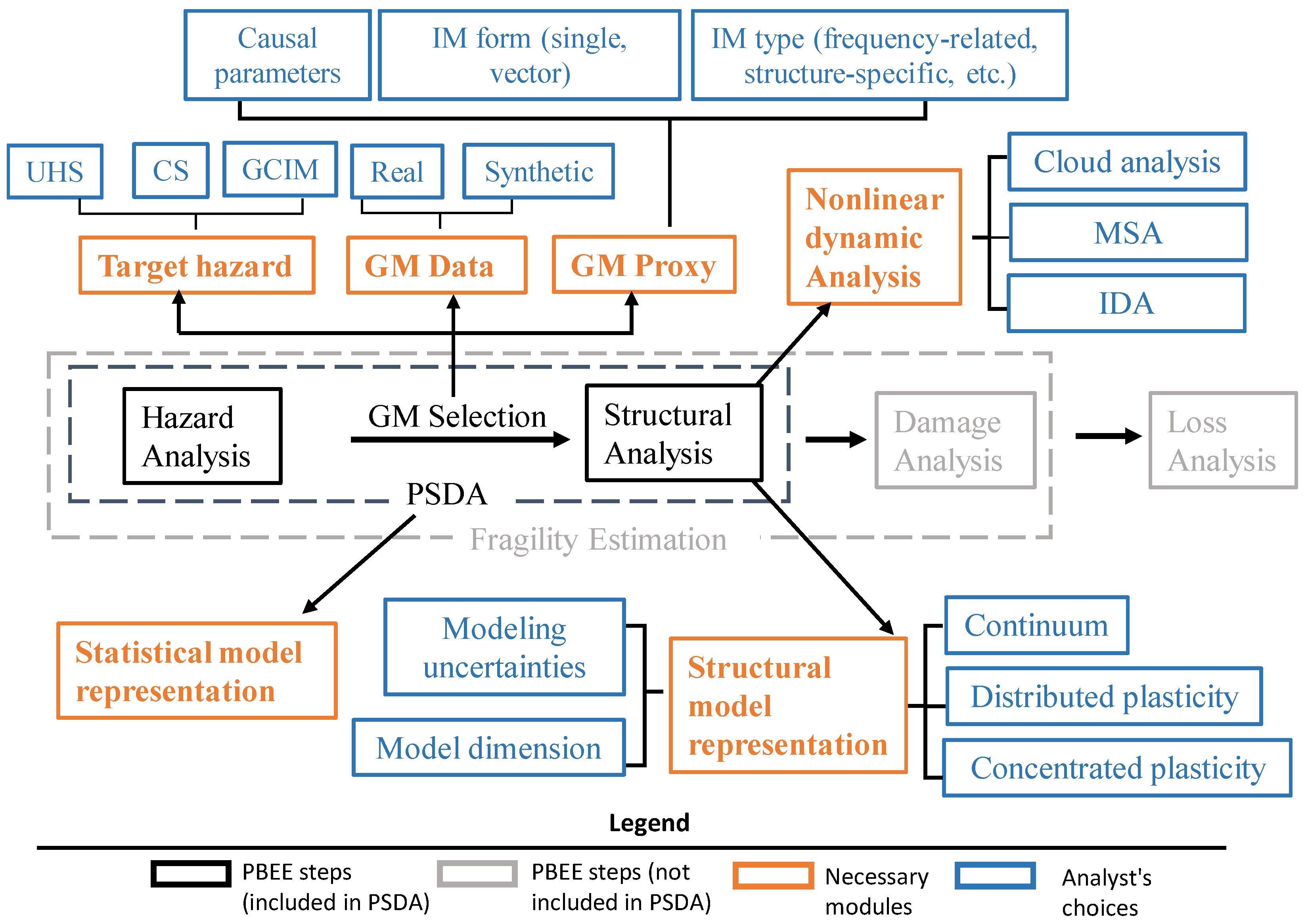
Table 1.
Proposed criteria to assess IMs suitability.
| IM Criteria | Definition | Calculation |
|---|---|---|
| Efficiency | Smaller variability of EDP|IM | The variance of residuals of EDP regression on IM |
| Sufficiency | Independency of EDP|IM of any other seismological variable (e.g., M, R) | the p-value of regressing residuals of EDP|IM on M and R, Information gain |
| Practicality | Dependency of EDP on IM | Regression slope of EDP versus IM |
| Hazard computability | Efforts to calculate the IM hazard curve | Qualitative measure |
| Scaling robustness | Lack of bias in the estimated EDP from scaled IMs | Regressing residuals of EDP|IM on scale factors |
| Proficiency | Proficiency + Efficiency | The ratio of the variance of EDP|IM residuals to the regression slope |
Table 2.
Proposed IMs for different structural systems.
| References | Structure | No. of Story | Studied IM(s) | Criteria a | Results |
|---|---|---|---|---|---|
| Cordova et al. [73] | Composite and steel frame | 6,12 | S* | E | S* estimates structural response with lower dispersion. |
| Luco and Cornell [59] | Steel frames | 3,9,20 | IM1E, IM1I, IM1E&2E, IM1I&2E | E, S | IM1I&2E is the most sufficient and efficient IM. |
| Bianchini et al. [89] | Steel frames | 6,12,18 | Saavg | E, S, SR, HC | Saavg performs better than Sa. |
| Lin et al. [74] | RC frames | 4,10,16 | SN1, SN2 | E, S, SR | SN1 and SN2 perform better Sa for short- and long-period structures. |
| Akkar and Özen [90] | SDOFs | - | PGV, PGA, PGV/PGA, Sa | E | PGV outperforms other IMs. |
| Yakut and Yilmaz [91] | RC frames | 2,7,9 | 11 different scalar IMs | E | For frames with periods between: (i) 0.2 s–0.5 s: PGA, VSI, Ic. (ii) 0.5 s–1.1 s: VSI, HI, Sa |
| Mollaioli et al. [92] | RC base-isolated frames | 4,6 | 14 non-structure-specific and 13 structure-specific IM | E, S | MVEIr SI (None of the studied IMs were sufficient) |
| Lucchini et al. [93] | A 3D Irregular RC frame | 3 | Several scalar and vector IMs | E | Sa(T1) and {ɛ, Sa(T1)} show poor performance. {Sa,x(T1,x),Sa,y(T1,y)} is a suitable for multi-directional response. |
| Luco et al. [94] | Non-ductile steel frames | 3,9,20 | PGA, PGV, PGD, Sa(T1), Sv(T1), Sd(T1), PSV(T1), TP | E, S | {Sa(T1), (Sa(T2)/Sa(T1)}, Sd(T1)/Sa(T1)} is sufficient. |
| Ebrahimian et al. [67] | Bare and Base-isolated RC frame | 4,6 | 32 scalar IMs and 6 vector IMs | E, S | {Sa(T1), RT1,T2, ɛ} is suggested for displacement-based responses. |
| Donaire-Ávila et al. [95] | RC frame with hysteretic dampers | 6 | 16 non-structure specific and 18 structure-specific IMs | E, S | Modified integral-based IMs (e.g., Housner) for displacement-based responses. |
| Barbosa [96] | 3D wall-frame | 13 | IM1={Sa(T1),Sa(1.5T1)} IM2={Sa(T1),Sa(T2)} | E, S | IM1 and IM2 for displacement- and acceleration-based EDPs, respectively. |
| Fagella et al. [97] | 3D RC building | 4 | SaY(T1), SaY(1.5T1), SaY(2T1), SaY(T4), PGAY, SaX(T2) | E, S | None of the scalar IMs were sufficient and efficient. Vector IMs are preferred. |
| Shokrabadi et al. [98] | Rocking braced frame w/ infills | Sa(T1), PGA, Saavg, Sdi | E, S | Saavg is suitable for peak and residual story drift. | |
| Yang et al. [99] | High-rise frame-core tube | 17,22 | 25 scalar IMs | E, S | PGV and MSI are suggested for peak drift. MVSI is suitable for isolator damage |
a Criteria: Efficiency (E), Sufficiency (S), Scaling robustness (SR), Hazard computability (HC).
Table 3.
Suggested minimum number of records.
| References | Proposed Minimum Number | Studied Structure | Comment |
|---|---|---|---|
| Eads et al. [115] | 40 | A 4-story frame | The confidence interval of the mean annual frequency of collapse |
| Kiani et al. [116] | 20 | 4-,8-, and 16-story buildings | If used with a hazard-consistent GM method |
| Baltzopolous et al. [117] | 40–100 | Three SDOFs and two 4-story frames | Using the Cornell reliability method |
| Sousa et al. [118] | 60 | A building portfolio | Compared to a GCIM-based suite with 150 records |
Publisher’s Note: MDPI stays neutral with regard to jurisdictional claims in published maps and institutional affiliations. |
© 2022 by the author. Licensee MDPI, Basel, Switzerland. This article is an open access article distributed under the terms and conditions of the Creative Commons Attribution (CC BY) license (https://creativecommons.org/licenses/by/4.0/).
Share and Cite
MDPI and ACS Style
Zaker Esteghamati, M. A Holistic Review of GM/IM Selection Methods from a Structural Performance-Based Perspective. Sustainability 2022, 14, 12994. https://0-doi-org.brum.beds.ac.uk/10.3390/su142012994
AMA Style
Zaker Esteghamati M. A Holistic Review of GM/IM Selection Methods from a Structural Performance-Based Perspective. Sustainability. 2022; 14(20):12994. https://0-doi-org.brum.beds.ac.uk/10.3390/su142012994
Chicago/Turabian StyleZaker Esteghamati, Mohsen. 2022. "A Holistic Review of GM/IM Selection Methods from a Structural Performance-Based Perspective" Sustainability 14, no. 20: 12994. https://0-doi-org.brum.beds.ac.uk/10.3390/su142012994
Note that from the first issue of 2016, this journal uses article numbers instead of page numbers. See further details here.