Spatio Prediction of Soil Capability Modeled with Modified RVFL Using Aptenodytes Forsteri Optimization and Digital Soil Assessment Technique

Abstract

To meet the needs of Egypt’s rising population, more land must be cultivated. Land evaluation is vital to achieving sustainable agricultural production. To determine the soil capability in the northeast Nile Delta region of Egypt, the present study introduces a new form of integration between the Agriculture Land Evaluation System (ALES Arid) model and the machine learning (ML) approach. The soil capability indicators required for the ALES Arid model were determined for the 47 collected soil profiles covering the study area. These indicators include soil pH, soil salinity, the sodium adsorption ratio (SAR), the exchangeable sodium percentage (ESP), the organic matter (OM) content, the calcium carbonate (CaCO₃) content, the gypsum content, the clay percentage, and the slope. The ALES Arid model was run using these indicators, and soil capability indexes were obtained. Using GIS, these indexes helped to classify the study area into four capability classes, ranging from good to very poor soils. To predict the soil capability, three machine learning algorithms named traditional RVFL, sine cosine algorithm (SCA), and AFO were also applied to the same soil criteria. The developed ML method aims to enhance the prediction of soil capability. This method depends on improving the performance of Random Vector Functional Link (RVFL) using an optimization technique named Aptenodytes Forsteri Optimization (AFO). The operators of AFO were used to determine the best parameters of RVFL since traditional RVFL is sensitive to parameters. To assess the performance of the developed AFO-RVFL method, a set of real collected data was used. The experimental results illustrate the high efficacy of AFO-RVFL in the spatial prediction of soil capability. The correlations found in this study are critical for understanding the overall techniques for predicting soil capability.

1. Introduction

On a worldwide scale, agriculture, industry, and services are the three main sectors involved in production, required for economic and sociocultural progress [1]. In relation to nutrition, the agricultural sector holds a distinctive place and significance among these sectors [2]. Numerous problems across the world, such as climate change, the depletion of water supplies, and the rapid increase in the population, are aggravating the demand for productive agricultural areas [3]. On the one hand, there is no increase in the amount of agricultural land used for production, and on the other hand, the quality of the land in use is degrading over time owing to the use of unscientific methods, leading to a decline in sustainability concurrently with output [4]. The difficulties farmers face every day are related to how, where, and when to cultivate. In essence, land capability refers to a soil’s ability to cultivate crops and grassland plants for an extended time frame without deterioration [5]. The capability of soil to support crop growth is influenced by its physical, chemical, and fertility properties [6]. All these properties also have a significant impact on soil fertility, and as a result, soil productivity also varies [7]. On the basis of the capability of the soil, farmers are required to predict food production and plan sustainable land management [8]. Land capability is a helpful tool to classify management zones intended for appropriate land use [9]. The capability evaluation of alluvial soils in the Nile Delta of Egypt is important, especially after long periods of intensive agricultural practices and loss of Nile sediments [10]. Anthropic activities may magnify soil degradation, which leads to situations that put soil productivity at risk [11].

It is one of the most important agricultural areas in Egypt. It suffers from deterioration mainly due to intensive cropping [10,11]. Additionally, due to land reclamation programs, agricultural land has increased, particularly in the northeastern zones around El-Manzala Lake and the northwestern parts. This expansion of agricultural land, however, was unable to cover the loss of formerly cultivated area to urban growth. Additionally, it was noted that before 2011, urban areas largely came up around older towns and cities; after 2011, however, they adopted a random distribution [12]. Nevertheless, our observations can provide a research direction to advance a strategy for soil capability prediction. In different regions of the world, land capability has been determined using different evaluation models mainly based on GIS software, such as the applied system of land evaluation (ASLE), the Mediterranean land evaluation information system (MicroLEIS), the land evaluation and site assessment system (LESA), and the land classification system of Storie index [13,14]. Land capability has also been classified using a multi-thematic approach, multivariate statistics, and ALES Arid [8,10,15]. The Geographic Information System (GIS) can also be used to analyze and map large amounts of spatial data and provide accurate and easily accessible information of different characteristics of soil and water [16,17]. Moreover, soil spatial variability is a vital tool used to obtain accurate classes of land capability [18,19].

To determine land capability, the present work uses a new form of integration of one of the land evaluation models, i.e., the Agriculture Land Evaluation System for arid and semi-arid regions (ALES Arid), and machine learning algorithms. The ALES Arid model is based on the Storie index, which has been modified by [19]. The Storie index is an acceptable and widely known soil evaluation method for land use and productivity worldwide [20]. The ALES Arid software can be incorporated with GIS to show its outputs in map form. A land capability map can be used to visualize which locations are best suited for which crops [21]. This model is one of the most recently developed methodologies that are practical for use in arid and semi-arid regions, so it is appropriate for Egyptian circumstances.

Machine learning is a methodological approach that executes the framework of an analytical model [22]. It belongs to the artificial intelligence field. Machine learning (ML) procedures have been prevalent in a variety of research sectors, particularly in the past 10 years [23]. Recently, a variety of machine learning methods have been used to identify soil features [24,25]. Several studies on soil assessment have been conducted using machine learning approaches [26,27]. Machine learning techniques are used to estimate soil distribution and quality indexes [28]. Machine learning approaches have also been demonstrated to be efficient for assessing and mapping various types of water-induced soil erosion [29,30]. However, it is currently uncertain how well machine learning systems can forecast soil capability. In this regard, to predict the soil’s capability, we used data on soil properties in the ALES Arid software. Then, we tested the same data in different models of machine algorithms, i.e., AFO, RVFL, and SCA. On the basis of the accuracy, sensitivity, and specificity of the data, we chose the model that is best for predicting land capability. Furthermore, the current study is the first global view on the role of machine learning algorithms in estimating soil capability. In the present work, the Dakahlia governorate in the northeast Nile Delta of Egypt was selected to apply the proposed integration.

2. Materials and Methods

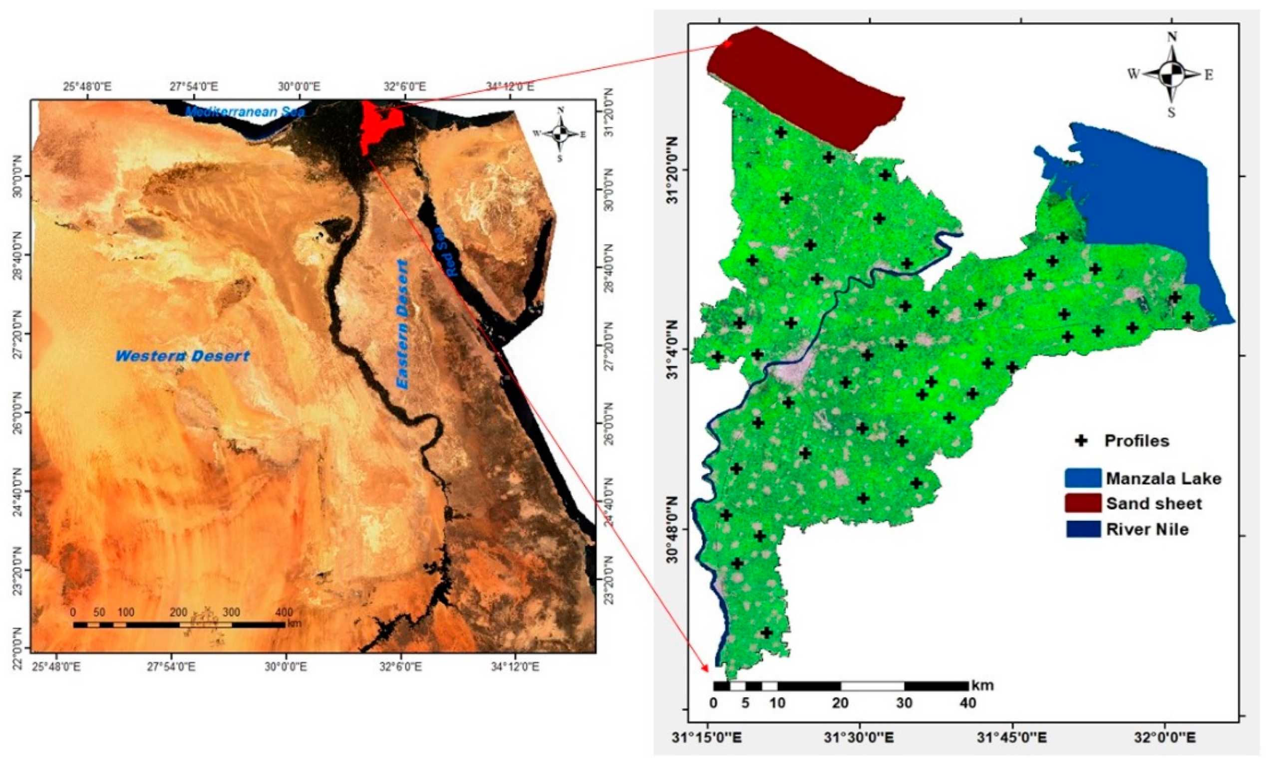
2.1. The Investigated Area

This study was conducted in the northeast Nile Delta, in the catchment area of Dakahlia governorate, Egypt, (31°12′47″ and 32°07′25″ E and 30°35′10″ and 31°34′02″ N), with an area of 3936 km² (Figure 1). The area has a Mediterranean climate, with daily temperatures oscillating between 15 and 33 °C and a mean annual temperature of 20 °C. The average annual rainfall is 57 mm and occurs mostly during the winter months. This indicates that the study area belongs to a thermic temperature and Torric moisture regime. The prevalent slopes change from 0 to 36 degrees, indicating that the majority of this area is leveled (Figure 2a). The elevation fluctuates from −35 to 45 m above sea level (Figure 2b). The geology of the studied area includes Nile deposits, sabkha deposits, and sand dunes [31]. In [32], the area is mainly described as a clayey alluvial deposit, except the northwestern parts, which are characterized by fluvio-marine deposits. To understand the broad soil pattern characteristics, a reconnaissance survey was carried out throughout the investigated area. Thereafter, on the basis of the pre-field interpretation and the data obtained from the survey, the soil profiles were selected to cover the morphological units of the study area as well as the variations in the field landscape.

2.2. Sampling and Soil Analyses

In all, 47 soil profiles were surveyed using GPS. Each soil profile includes 3 or 4 horizons. One soil sample was collected from each horizon for different analysis. Most of the soil profiles were dug to a depth of 150 cm or to the permanent water table. Some profiles were 100 cm deep and located in sabkha deposits. In the studied area, the horizon depth differs across the soil profiles on the basis of morphological aspects, observed in the field survey, such as color, texture, and boundaries. The soil samples were put through a 2 mm sieve after being air-dried and crushed to prepare them for physical, chemical, and fertility analyses according to standardized protocols described in [33,34].

2.3. The ALES Arid Software

The ALES Arid software is based on the Storie index, which evaluates land capability using four indexes, A, B, C, and X, where A is for soil’s physical properties, including soil profile depth (cm); B is for soil texture; C is for slope; and X is for other soil factors, including calcium carbonate content, gypsum content, irrigation water quality, topographic, drainage, fertility, nutrient level, climate data, topography, and alkalinity. A score ranging from 0 to 100% is determined for each index, and the scores are then multiplied together to generate a final index expressing the soil capability class [35].

Using Equation (1), the soil data were transformed into weighted average values (av) for each soil characteristic, which was associated with a specific soil profile. To calculate the weighted average values, the number of soil horizons, the horizon thickness, and the total soil depth were obtained for each soil profile:

$$av=\left(\frac{{{\displaystyle \sum }}_{i=1}^n\left(v_i{t}_i\right)}{T}\right),$$

(1)

where v_i denotes the value of soil property for the soil horizon i, t_i is the soil horizon thickness, n is the number of soil profile horizons, and T is the total depth of the soil profile.

The capability index and limitations for each parameter were calculated using weighted average values of soil parameters and proposed ratings coded within the model (

Table 1. Land capability classes, grades, and capability indexes of ALES Arid software [20].

Capability Class	Grade	Capability Index (%)
C1	Excellent	80–100
C2	Good	60–79
C3	Fair	40–59
C4	Poor	20–39
C5	Very Poor	10–19
C6	Nonagricultural	<10

). If a parameter’s index is less than 50%, the parameter is considered a limiting factor (Equations (2) and (3)).

$$Log\left(MI\right)=\frac{\log \left(I_1{I}_2{I}_3\dots \right)}{n},$$

(2)

$$MI=antLog\left(MI\right),$$

(3)

Here, MI is the major index; I₁, I₂, and I₃ are the inner estimated indices; and n is the number of the inner indices used for the major index calculation. After calculating the three major land capability indexes, the model computes the final land capability index from the three major indexes. Finally, the model categorizes the land capability classes on the basis of the proposed capability classifications provided in Table 1.

2.4. Data Sets

The investigated area is covered by two Landsat 8 (OLI-TIRS) scenes (path 176, rows 38 and 39) acquired on 9 August 2020. Images were mosaicked to acquire a single image using a histogram matching and stitching process. The mosaicked image was subsetted to cover the study area and its outside boundaries. The satellite image was corrected atmospherically and radiometrically to enhance the image quality. The digital elevation model (DEM) of the study area was extracted from the Shuttle Radar Topography Mission (SRTM) images. The slope degree was computed using the DEM and spatial analysis tools in ArcMap 10.4 software (Esri, Redlands, CA, USA).

2.5. GIS Spatial Mapping

To create a geodatabase for the input data of soil properties, the software ArcGIS 10.3 (Esri, Redlands, CA, USA) was used. To create spatial distribution maps of the collected soil profiles in a raster format, the locations of the soil profiles were geo-referenced, converted to shapefile format, and interpolated. The inverse distance weighted (IDW) interpolation was used to create these maps using the GIS spatial analyst tool [36]. To produce a representative interpolation of the points, the IDW needs a lot of points (>14 soil profiles) [36]. IDW performs best when the soil profiles points are evenly dispersed throughout the region, and not clustered [37]. IDW assumes that the rate of correlations between nearby points is proportional to the distance between them [38]. The concept that objects are more similar to one another when they are close to one another is clearly implied through IDW interpolation [39]. When sampling is sufficiently dense in relation to the local variation that we are attempting to simulate, the best results from IDW are obtained [40]. According to the ArcGIS^® software by Esri, ArcGIS^® and ArcMap™, the IDW method is an advanced and accurate interpolation geostatistical procedure, and it is commonly used in soil, water resources, and geological sciences. Soil mapping has been used in several studies on soil assessment using IDW interpolation [36,41].

In the current study, IDW was used to estimate properties at a point i and Pi was based on property values at measured locations, where $Pi$ is the property at the soil profile location $i$, $Pj \mathrm{is} \mathrm{the} \mathrm{property} \mathrm{at} \mathrm{the} \mathrm{soil} \mathrm{profile} \mathrm{location} j$, $D_{ij}$ is the distance from $i$ to j, $G$ is the number of soil profile locations, and n is the inverse distance weighting power. The property at each unknown location is given by Equation (4):

$$P_i={\displaystyle \sum }_{j=1}^G\frac{Pj}{D_{ij}}n {\displaystyle \sum }_{j=1}^G\frac{1}{D_{ij}}n.$$

(4)

2.6. Machine Learning Models

2.6.1. Random Vector Functional Link

The Random Vector Functional Link (RVFL) connects input and output nodes as in the feedforward neural networks (Figure 3) [42]. The weights of the output layer are edited during the process. The weights are randomly generated and do not need to be modified. These features help in improving the prediction performance and avoiding the overfitting issue that can appear in traditional artificial neural network (ANN) models.

The RVFL processes start when the input data are fed to the input nodes. These data include $M$ soil profiles designed as $(a_i, b_i)$, where $a_i\in R^n, b_i\in R^m, i=1,\dots ,M$. Then, the output of the hidden layer is computed by the following equation:

$$O_j\left(c_j{a}_i+d_j\right)=\frac{1}{1+e^{-\left(c_j{a}_i+d_j\right)}} , d_j\in \left[0,\xi \right], c_j\in \left[-\xi ,\xi \right].$$

(5)

In Equation (5), $\xi$ represents the scalar values and $c_j$ and $d_j$ are the input weights between hidden and input nodes and the bias, respectively. RVFL predicts the output using the weight $w$ and is calculated as:

$$Z={\rm K}w,w\in R^{n+P},$$

(6)

where ${\rm K}=\left[{{\rm K}}_1,{{\rm K}}_2\right]$ exemplifies the input data, and ${{\rm K}}_1$ and ${{\rm K}}_2$ are defined as

$${{\rm K}}_1=\left[\begin{array}{ccc}{a}_{11}& \dots & a_{1n}\\ ⋮& \ddots & ⋮\\ a_{N1}& \dots & a_{Nn}\end{array}\right], {{\rm K}}_2=\left[\begin{array}{ccc}{O}_1\left(c_1{a}_1+d_1\right)& \dots & O_P\left(c_P{a}_1+d_P\right)\\ ⋮& \ddots & ⋮\\ O_1\left(c_1{a}_N+d_1\right)& \dots & O_P\left(c_P{a}_N+d_P\right)\end{array}\right],$$

(7)

The $w$ is modified using the following equation:

$$w=K^{†}Z,$$

(8)

In Equation (8), $†$ denotes the Moore–Penrose pseudo-inverse [26].

2.6.2. Aptenodytes Forsteri Optimization Algorithm

The AFO algorithm mimics emperor penguins in huddling for warmth [43]. They have some strategies based on their fat and the temperature of the environment. They are looking for a heating location to move toward energy and temperature. In AFO, the positions of the penguins represent the solutions X used to determine the parameters of RVFL, and their temperature is the fitness function Y. Therefore, the best fitness is the highest-temperature location.

• Move mode I: Temperature sensing

The gradient estimation method of position is as follows: At the time $t$, for the $i$th penguin, the position is $X_i^t=\left[x_1,\dots ,x_j,\dots ,x_D\right]$ and its corresponding fitness (temperature) is $Y_i^t$ [43]. The position is $X$ after minimal movement in the $i$th axis, and its fitness is $Y$. The position is $X_{ij}^{{}^{\prime }t}=\left[x_1,\dots ,x_j+\Delta x,\dots ,x_D\right]$ after minimal movement in the $i$th axis, and its fitness is $Y_{ij}^{{}^{\prime }t}$. Then, the partial derivative of the current position in the $j$th direction can be formulated as [43]:

$$g_{ij}^t=(Y_{ij}^{\prime }-Y_i)\Delta x,$$

(9)

where $g_{ij}^t$ is the partial derivative of each axis direction, which is estimated by:

$$G_i^t=\left[g_1,g_2,\dots ,g_D\right],$$

(10)

After that, the penguin’s displacement $A{T}_i^t$ on the basis of temperature perception can be obtained by:

$$A{T}_i^t=\alpha G_i^t,$$

(11)

where $\alpha$ defines the conversion factor from the gradient of the temperature to displacement.

• Move mode II: Reference to memory

In the search process, the penguins will remember the position they had visited and the temperature of that position. $X{m}_i^t$ denotes the location of the optimal fitness $Y{m}_i^t$ in the penguin’s memory at time $t$. The following equation describes the calculation of the penguin’s displacement to explore a new position influenced by memory.

$$A{M}_i^t=R_1\beta \left(X{m}_i^t–X_i^t\right),$$

(12)

where $R_1$ denotes a random number.

• Move mode III: Reference to other individuals’ locations

The displacement of penguins is influenced by other penguins. In the penguin population, the locations of two penguins are $X_p^{t}1$ and $X_p^{t}2$, and the corresponding functions are $Y_{p1}^t$ and $Y_{p2}^t$. At time $t$, the following equation formulates this movement:

$$A{l}_i^t=R_2\gamma (X_{p1}^t-X_{p2}^t)\left(-sgn(Y_{p1}^t-Y_{p2}^t)\right),$$

(13)

$$\gamma =2arctanh(1-\frac{t}{T_{max}}),$$

(14)

where $R_2$ is a random number, sgn(X) controls the positive and negative values of variable $X$, and $t$ and $T_{max}$ are the iteration and the max iteration number, respectively.

• Move mode IV: Movement to the population center

While the penguins are huddling for warmth, they try to move toward the center of the population (the warmest position, $c^t$). The following equation shows this movement:

$$A{C}_i^t=R_3\delta \left(X{c}^t–X_i^t\right),$$

(15)

where $R_3$ is a random array and $\delta$ is a control factor.

• Move mode V: Minimization of energy consumption

Penguins try to reduce unnecessary actions, and their displacement at time $t$ will be less than what occurred previously, at time $t-1$. If the displacement at the previous moment is $A_i^{t-1}$, the displacement $A{V}_i^t$ at time $t$ can be calculated as follows:

$$A{V}_i^t=\epsilon A_i^{t-1},$$

(16)

where $\epsilon$ is a coefficient and controls the previous displacement at time $t-1$.

• Final displacement

The final displacement $A_i^t$ is the weighted sum of the above five displacements

$$A_i^t={\omega }_{1}A{T}_i^t+{\omega }_{2}A{M}_i^t+{\omega }_{3}A{l}_i^t+{\omega }_{4}A{C}_i^t+{\omega }_{5}A{V}_i^t,$$

(17)

$$X_i^t=X_i^{t-1}+A_i^t,$$

(18)

where $X_i^t$ is the new position of the penguins and $\omega$ is the weight of the displacements.

2.6.3. Designing the Algorithm Further

This section presents different updated approaches for penguins.

• Gradient estimation in the exploration stage

In this stage, the gradient is estimated by the increment $\Delta x\left(step\right)$ of $X$. A change in the gradient estimation step size balances development and exploration. The following equations show this change in step size:

$$c=exp\left(-30\times \left(t-Gap0\right)/T_{max}\right),$$

(19)

$$\Delta x=c\left|\left|S_{max}-S_{min}\right|\right|/2,$$

(20)

Here, $c$ is a coefficient that denotes the changing gradient estimation step, $S_{max}$ and $S_{min}$ are the penguin displacement range, and $Gap0$ is the initial use period for the method.

• More accurate gradient estimation

This method is applied to add more flexibility to the gradient estimation method. It solves the potential errors due to minus steps in the gradient estimation method, as in the following equations:

$$g_{ij}^t=\frac{Y_{ij}^{{}^{\prime }t}-Y_i^t}{\Delta x}+\frac{Y_{ij}^{{}^{″}t{}^{\prime }}-Y_i^t}{-\Delta x}=\frac{Y_{ij}^{{}^{\prime }t}-Y_{ij}^{{}^{″}t{}^{\prime }}}{\Delta x},$$

(21)

where $g_{ij}^t$ is the partial derivative for each direction. The partial derivatives $G_i^t$ for the solution can be calculated as:

$$G_i^t=\left[g_{i1}^t,\dots ,g_{iD}^t\right],$$

(22)

• Usage interval of move mode I

This approach is used more frequently in the exploitation stage of the algorithm. This mode interval decreases gradually with the increase in iterations. The interval is formulated by the following equation:

$$Ga{p}_{i+1}=max\left(Ga{p}_i-dec,Ga{p}_{min}\right),$$

(23)

where $Ga{p}_i$, $Ga{p}_{min}$, and $dec$ are the use interval, the minimal value of use interval, and a decrement of use interval, respectively.

• Adaptive multi-step update based on estimated gradient

This approach is used to extend the updating method. The algorithm can apply the remainder of the estimated gradient evaluation time periods to test the difference, as in the following equation:

$$M=2-2D,$$

(24)

where $N$ is the population size, $D$ is the dimension, and $2D$ is the estimated gradient evaluation time period.

If there is a magnitude difference between the objective function and the decision variables, the following equation is used:

$$g_{ij}^t=\frac{log(Y_{ij}^{{}^{\prime }t})-log(Y_i^t)}{\Delta x}+\frac{log(Y_{ij}^{{}^{″}t{}^{\prime }})-log(Y_i^t)}{-\Delta x}=\frac{log(Y_{ij}^{{}^{\prime }t})/log(Y_{ij}^{{}^{″}t{}^{\prime }})}{\Delta x},$$

(25)

On the basis of the above equation, the $G_i^t$ for the solution can be calculated as:

$$G_i^{{}^{\prime }t}=\frac{G_i^t\left|\left|S_{max}-S_{min}\right|\right|}{2\left|\left|G_i^t\right|\right|},$$

(26)

$$X{c}_i^t=X{c}_i^{t-1}+\alpha G_i^{{}^{\prime }t},$$

(27)

$${\alpha }_i=exp(-\frac{10\left(i-1\right)}{M-1})(1-\frac{\left(i-1\right)(1-\frac{\Delta x}{\left|\left|G_i^t\right|\right|})}{M-1}),$$

(28)

• Replacement strategy of mode I

This mode is proposed to extend the exploitability of the original move mode. It is formulated as in the following equation:

$$X_i^t=X_i^{t-1}+\frac{5Dm{R}_n}{\left|\left|R_n\right|\right|}),$$

(29)

$$Dm=\left|\right|\frac{{\sum }_{i=1}^N(X_i^t-X_c^t)}{N}\left|\right|$$

(30)

where $Dm$ is the distance between the penguin and the center.

The population updates should consider the number of iterations of the algorithm, as shown in the following equation:

$$Dm=\frac{\left|\left|S_{max}-S_{min}\right|\right|}{2},Dm=\frac{t\left|\left|S_{max}-S_{min}\right|\right|}{20T_{max}},$$

(31)

• Improved move mode III

This improvement works to replace some of the old solutions with the optimal ones. This phase is formulated as in the following equations:

$$A{l}_{ij}^t=R_2\gamma (X_{p1j}^t-X_{p2j}^t)\left(-sgn(Y{m}_{p1}^t-Y{m}_{p2}^t)\right),$$

(32)

$$A{l}_{ij}^t=R_n\gamma \left(S_{maxj}-S_{minj}\right)/2,$$

(33)

Here, $X_{p1j}^t$ and $X_{p2j}^t$ denote the best random solutions, $j$ is the dimension, and $Y{m}_{p1}^t$ and $Y{m}_{p2}^t$ denote the best temperature.

To prevent solutions from falling into the local optimum, the following equation is used:

$$std=\sqrt{{\displaystyle \sum }_{i=1}^N\left(X{m}_{ij-{\mu }_j}\right)/N},$$

(34)

If $std\le 0.5 exp\left(-20t/T_{max}\right)\left(S_{maxj}-S_{minj}\right)$, the following equation is used:

$$A{l}_{ij}^t=-0.5R_n\gamma \left(S_{maxj}-S_{minj}\right)sgn\left(Y{m}_{p1}^t-Y{m}_{p2}^t\right)\left(X_{p1j}^t-X_{p2j}^t\right),$$

(35)

• Discardable move mode V

This step uses Equation (24) to correct the current penguin’s movement.

• Alternate penguin moving strategies

This step depends on the weighted sum of the previous movement modes, as in the following equations:

$$A_i^t=w_{2}A{M}_i^t+w_{4}A{C}_i^t+w_{5}A{V}_i^t,$$

(36)

$$X_i^t=X_i^{t-1}+A_i^t,$$

(37)

where $w_2$ and $w_4$ = 1 and $w_2$ = 0.5.

The probability is applied to switch movements two and three. The following equation is used with movement three:

$$p_i=arctanh\left(\left|Y_i^t-Y_c^t\right|\right)\left(T_{max}-t\right)/T_{max,}$$

(38)

The probability of movement two is $1-p_i$.

• Catastrophic strategy

This strategy is used if the improvement is less than 1%, to regenerate solutions and clear the memory. The following equation is used to control this step:

$$count=count+1,\hspace{1em}0.99Y_c^{t-1}\le Y_c^t,$$

(39)

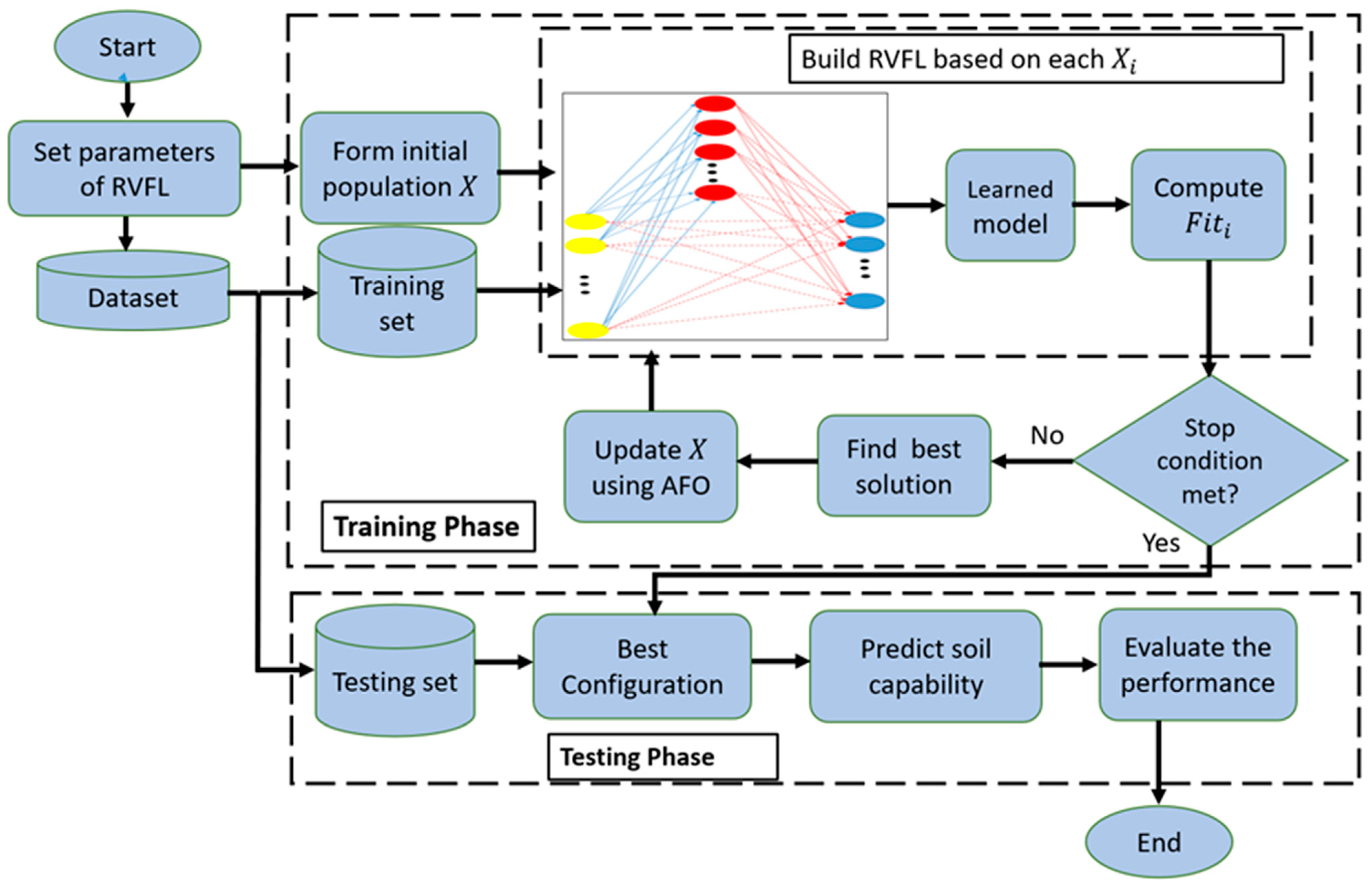
2.6.4. Proposed AFO–RVFL Method

In the AFO–RVFL approach, first, the data are divided into two parts: a 20% part for testing and an 80% part for training. Next, the initial population $X$ is created, consisting of $N$ solutions with $dim$ values, using Equation (40).

$$X_{ij}=l_j+r\times \left(u_j-l_j\right), i=1,\dots ,N,j=1,\dots ,dim,r\in \left[0,1\right],$$

(40)

where $X_i$ stands for the RVFL parameters, including three values: the activation function ($AF$), the randomization strategy ($RT$), and the number of hidden nodes ($N_h$). For example, $X_i=\left[AF,RT, N_h\right]$, where $AF\in \left\{1,2,3,4,5\right\}$ means the type of activation used, and it includes the radbas, tribas, sign, hardlim, and sig, respectively. The definitions of these transfer function are given as in

Table 2. Definition of activation function.

Function	Formulation
Radial basis (radbas)	F(n) =$e^{-n^2}$
Triangular basis (tribas)	F(n) =$\{\begin{array}{c}1-{\left|xn\right|}^2 -1<n<1\\ 0 otherwise\end{array}$
Sigmoid (sig)	$F\left(n\right)=\frac{1}{1 = e^{-n}}$
Hard-limit (hardlim)	$F\left(n\right)=1$ if $n\ge 0$
sign	$F\left(n\right)=\frac{\mathrm{n}}{\left|\mathrm{n}\right|}$

.

In addition, $N_h\in \left[1,2000\right]$ indicates the number of hidden nodes. $RT\in \left\{1,2\right\}$ stands for either the Uniform or Gaussian, and is used to construct the weights of the network.

Next, the fitness value ($Fi{t}_i$) of $X_i$ is computed and represents the error of classification using KNN classifiers. This can be formulated as:

$$Fi{t}_i=1-\gamma ,$$

(41)

where $\gamma$ is the accuracy of the classification using the KNN training set. Then, the best set of parameters (i.e., best solution) is determined and used with the operators of AFO to enhance the other solutions. The stop conditions are checked next, and if they do not meet the criteria, the updating process is repeated. Otherwise, we return to the best solution and evaluate it by constructing RVFL according to its value and using the testing set. The developed soil capability prediction steps are provided in Figure 3.

2.6.5. Performance Metrics

We evaluate the performance of the presented soil capability prediction model using different performance measures, such as accuracy, sensitivity, specificity, and precision. In addition, we compare it with other models, such as the sine cosine algorithm (SCA) and traditional RVFL. Accuracy, sensitivity, specificity, and precision are also used to evaluate the algorithm quality. These measures are defined as in

Table 3. The definition of performance metrics.

Measure	Formulation
Accuracy	$\frac{TP + TN}{TP + TN + FN + FP}$
Precision	$\frac{TP}{TP + FP}$
Sensitivity	$\frac{TP}{TP + FN}$
Specificity	$\frac{TN}{TN + FP}$

TP, TN, FP, and FN are the true positive, true negative, false positive, and false negative values in the data, respectively.

.

3. Results and Discussion

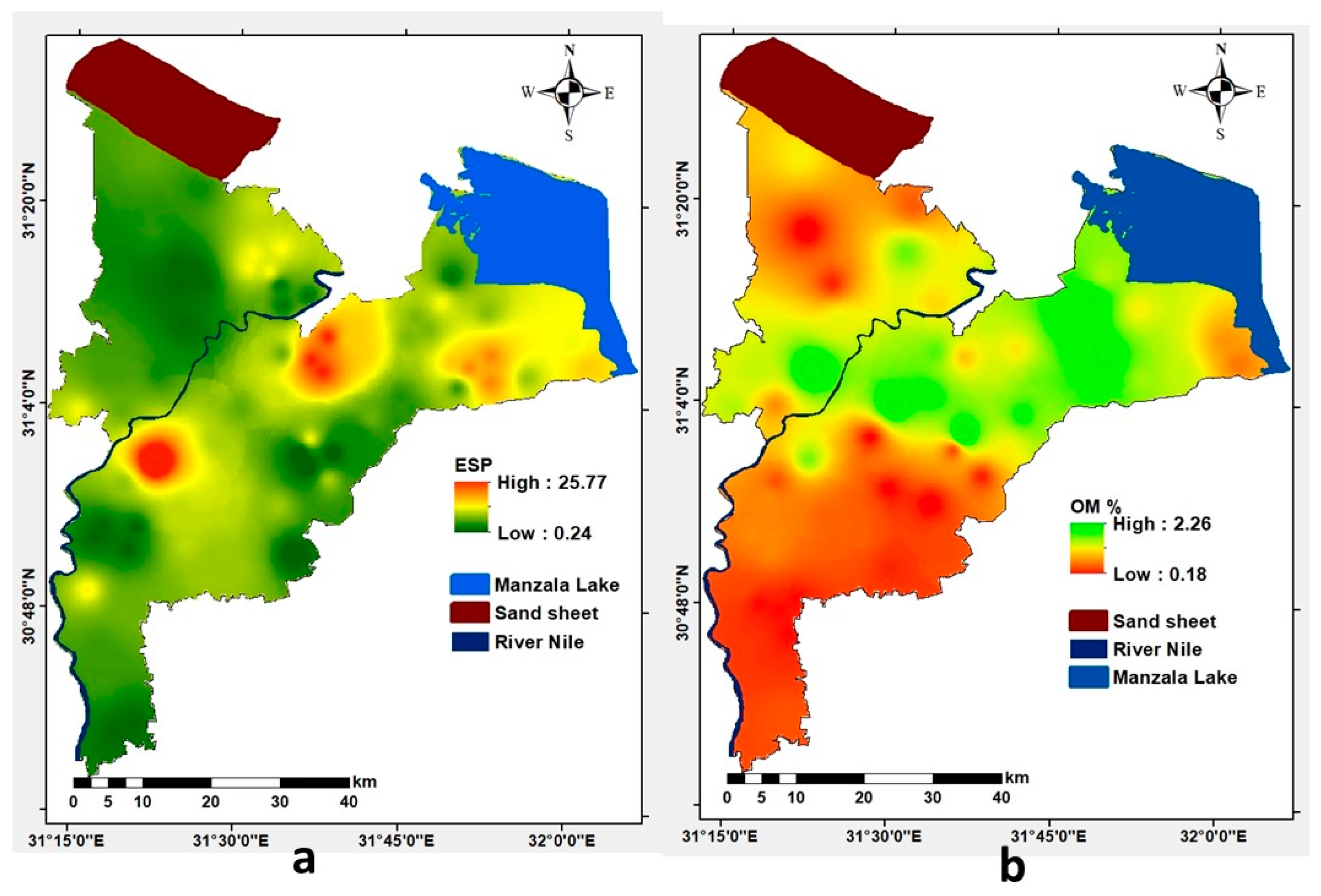
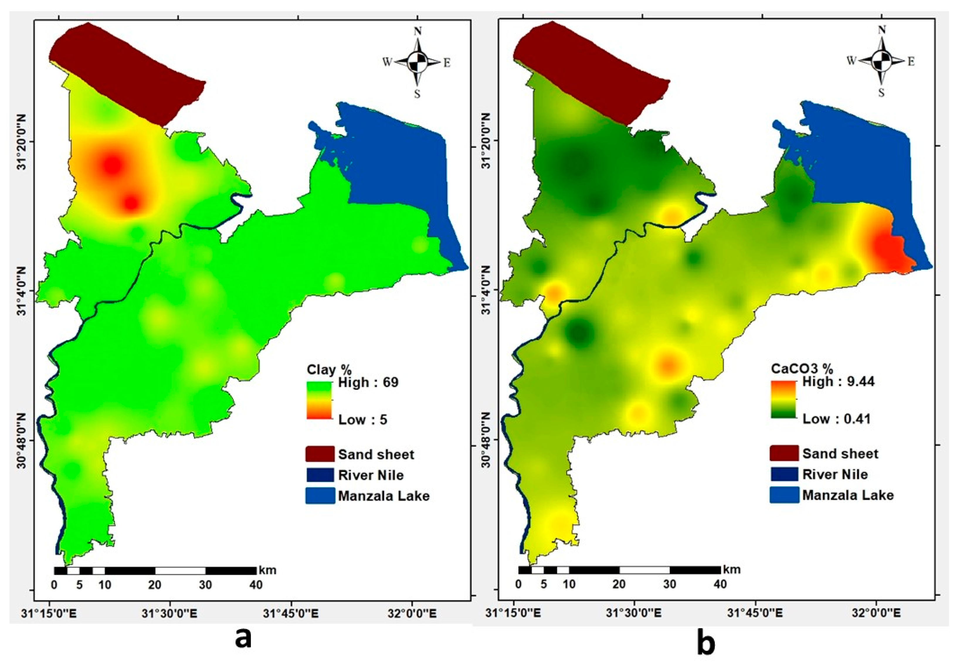
3.1. Soil Physicochemical Characteristics

The soils were moderately deep to very deep, and according to [44], ranged from 100 to 150 cm (Figure 4a). According to [45], the soils exhibited a neutral to strongly alkaline pH, ranging from 7.23 to 8.63 (Figure 4b). According to [45], the soils were non-saline to saline (Figure 5a). The EC values varied between 0.45 and 8.45 dSm⁻¹, with the exception of profile 44, which had an EC value of 28 dSm⁻¹ and was classified as strongly saline soil. Low soil salinity reflects advanced cultivation, which enhances leaching and free drainage conditions, resulting in high soil capability [46]. However, saline soils were found in the upper area near El-Manzala Lake, which was thought to be the main source of salinization in the northwestern parts of the study area [47,48]. Proximity to the coast and a progressive increase in subsidence encourage water infiltration, resulting in salinization, regarded as the beginning of low soil capability [48]. Thus, soil salinity is a critical issue in agriculture, affecting land evaluation the world over [9]. The sodium adsorption ratio (SAR) values of the study area were less than 13, excluding profiles 15 and 47, with values of 18 and 15, respectively (Figure 5b).

The exchangeable sodium percentage (ESP) values of the study area were less than 15%, except for profiles 15 and 47, which had values of 25.0 and 17.0, respectively (Figure 6a). Cultivation was observed to decrease SAR values, lowering ESP values and indicating that there was no alkalinity hazard [48]. Salinity and sodicity are major constraints on land capability and agricultural production [49]. The soil organic matter content (OM) was extremely low to moderate, ranging from 0.18 to 2.26% (Figure 6b). Due to the prevailing arid climate, there is a deficiency of organic matter [50,51]. Soils with a finer texture have more organic matter than soils with a coarser texture [51,52]. Low soil OM is one of the most important soil constraints, as OM has a direct impact on the soil properties and, most significantly, limits its capability [53,54].

Many farmers use natural fertilizers, such as manure, leaf mold, sawdust, straw, animal waste, green manure, and compost, to improve the soil capability status [55]. Several environmental factors have been linked with soil OM, including topography, climate, vegetation, and soil properties such as texture [46,56]. The clay percentage of the study area varied from 5 to 69%. Consequently, the texture of the majority of the soil was clayey, except for the soil near the coast, which was sandy (Figure 7a). Soil texture is an influential factor in soil and crop management [35]. Thus, soil texture is considered a severe limiting factor [57]. The CaCO₃ content ranged from 0.41 to 9.44% (Figure 7b). Gypsum content was very low, ranging from 0.09 to 4.40% (Figure 8a). According to [44], the studied soils were non-calcareous to moderately calcareous and non-gypsiric to slightly gypsiric. High values of calcium carbonate content in some profiles date back to the shell remnants (inert CaCO₃) and the original lacustrine deposits in these soils near El-Manzala Lake [21]. These restrictions on soil capability, and therefore crop productivity, in the study area are not insurmountable; they can be solved by using appropriate fertility and land management techniques [58].

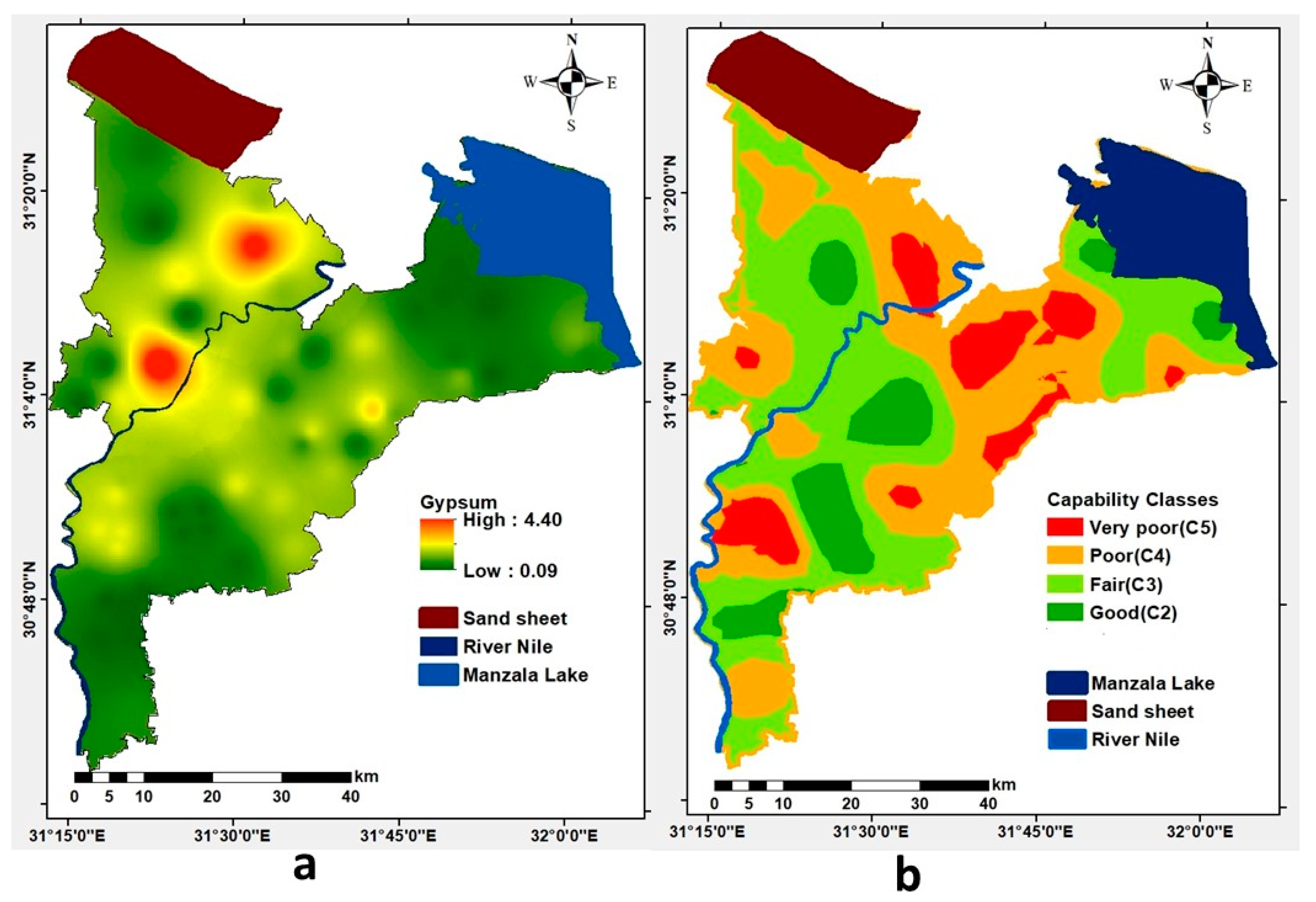
3.2. Soil Capability Map Predicted

After obtaining soil capability indexes and classes of 47 locations from the ALES Arid software (Table 1), IDW was applied to predict a spatial distribution map for soil capability (Figure 8b). The study area was classified into four classes (C2 to C5):

• In all, 11.31% (369.13 km²) of the studied area was determined as class 2 (C2), which is defined as good soil for agricultural crops, including alfalfa, wheat, barley, onion, sugar beet, sunflower, and pear. Class 2 requirements include a clayey texture, slightly alkaline soils, and low soil salinity (ECe ˂ 2 dSm⁻¹). The soils that belong to this class are characterized by advancements in agricultural management practices, high-quality irrigation water, and an effective soil drainage system, which all dramatically reduce soil salinity [21]. Therefore, these soils are suitable for a variety of plants, with no or only minor restrictions that limit the choice of species or require conservation activities [57];
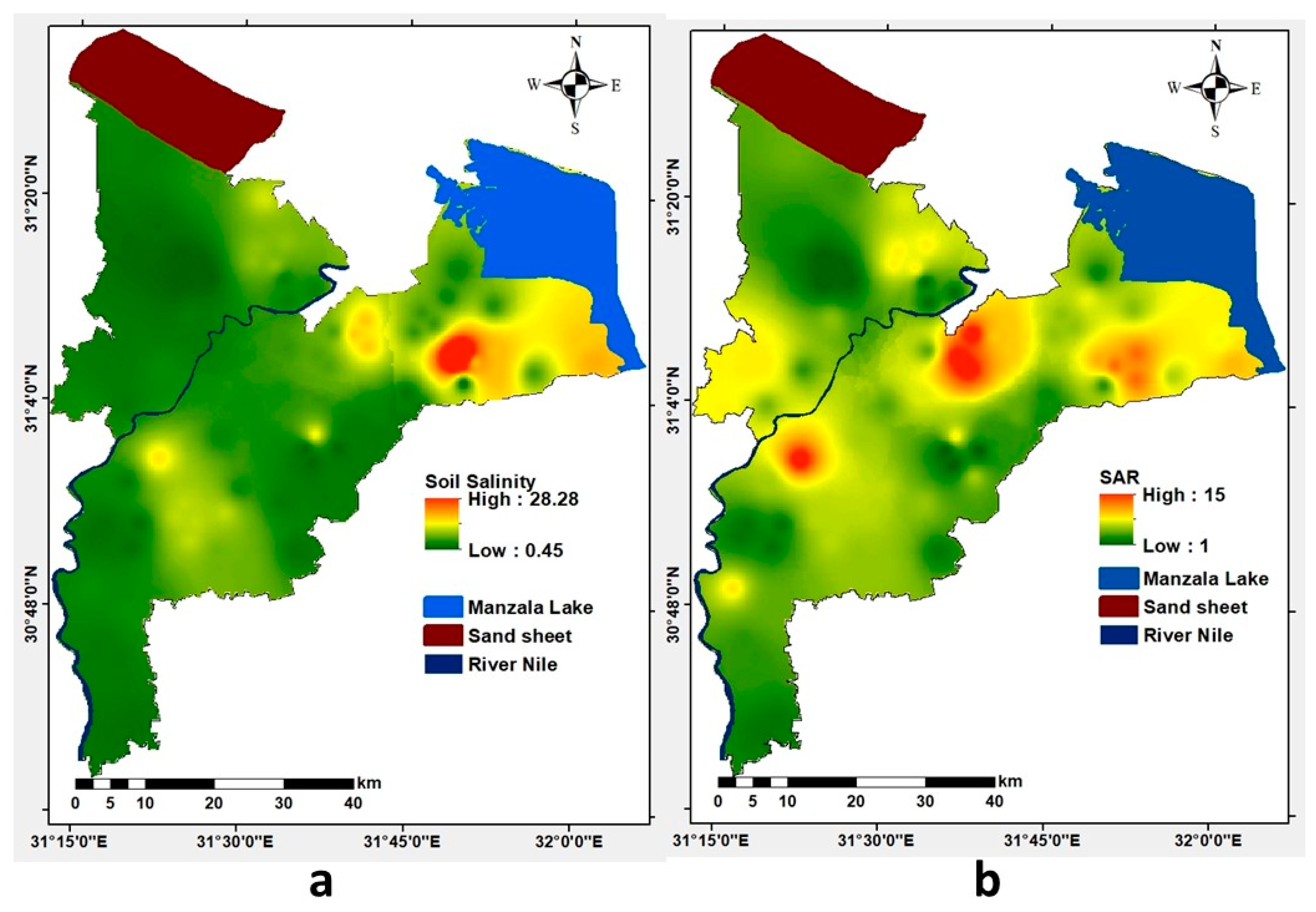
• The majority of the investigated area, or 42.87% (1398.25 km²), was defined as class 3 (C3), which is called fair soil. Class 3 soils have severe restrictions, ranging from one to five, that limit the available plants or necessitate conservation efforts, or both [15]. These soils have a slightly higher salinity, exceeding 4 dS cm⁻¹; higher alkalinity; and lower OM content than the soils of class 2 [59]. Additionally, the soils that belong to this class suffer from seawater intrusion from El-Manzala Lake [48]. However, the increase in salinization in these soils results from numerous factors, including drainage conditions, water table levels, and irrigation water types that have a negative influence by mixing with the saline drainage water due to a lack of irrigation water [60]. Furthermore, human engagement in agricultural management and climate change have a significant impact on the acceleration of salinization processes [61];
• About 35.19% (1147.77 km²) of the study area was classified as poor, class 4 (C4), soil. Compared with class 3 soils, these soils have more severe restrictions, ranging from three to five, which restrict the selection of plants, require careful management, or both [15,21,44]. The soil drainage networks in these regions are insufficient [26], and the condition of the soil drainage is one of the soil capability limiting factors that may prevent nutrients from freely moving and from being absorbed. It is important to emphasize that some agricultural techniques can improve soil capability and thus reduce restrictions [62]. To develop and protect these soils, more cautious management and conservation measures are required, such as using manure and irrigation water with low salinity. Such management can enhance the soil’s physical fertility, biological activity, and the soil OM content, which are associated with soil nutrients. Additionally, it can maintain the soil’s porosity while promoting deep drainage, which raises the soil capability [63,64];
• A small part of the study area, covering about 10.61% (346.26 km²) of the total area, was classified as very poor soil, or class 5 (C5). These soils have more severe limitations that make them generally unsuited to cultivation. Consequently, they are only suitable for fish pond usage. The main contributing factors to these soils include excessive irrigation; anthropogenic activity with natural drainage; improper timing of the use of heavy machinery; and a lack of conservation monitoring.

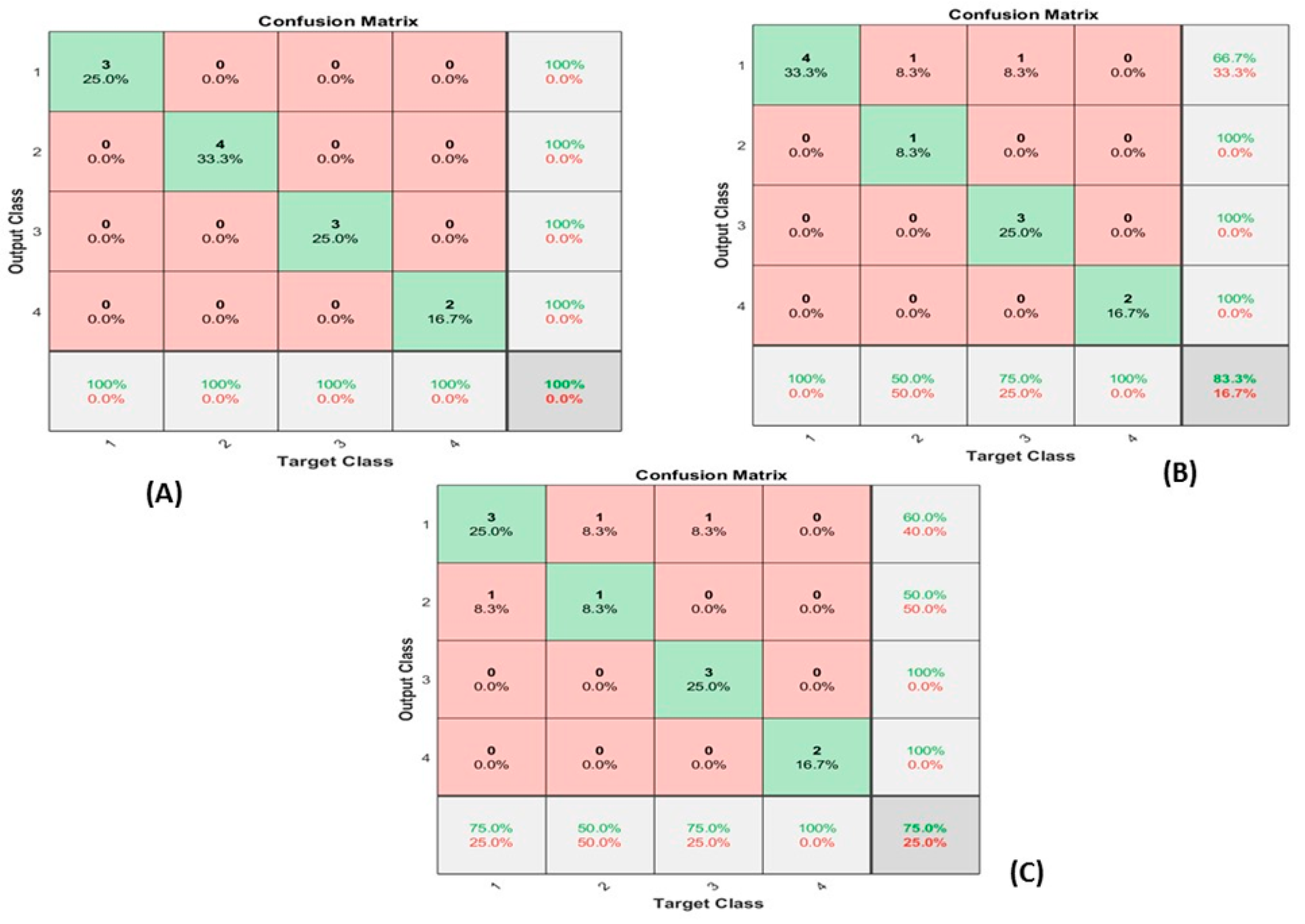
3.3. Uncertainty Assessment and Model Validation

Various factors may contribute to the model’s uncertainty: uncertainty resulting from the model and uncertainty resulting from scale-down precision and detail in data available at smaller scales [65]. Uncertainty in the predicted soil capability map may be linked to the significant variability in the data in terms of soil properties, the low accuracy of the covariates, the inherently poor relationships between the soil properties and the covariates, modeling mistakes, the number of the studied soil profiles in relation to the study area, and the effect of urbanization [66]. To validate the soil capability map of the study area, the map was checked with the soil quality map produced using a GIS-based model in accordance with the geometric mean algorithm, where the same study area was related to five grades: very high, high, moderate, low, and very low [67]. The results were found to be highly correlated, except for one class, i.e., grade 1. The suggested model provides for updating the database on the study area with the possibility of reporting in real time any changes in one or more of the cartographic topics covered (pH, salinity, SOM) [68]. Therefore, the soil capability map introduced with the applied model should not be considered as a permanent document but a modifiable one in a positive or negative sense, depending on anthropic interventions, urban density, and natural impacts, mainly climatic change. The prediction accuracy will need to be increased through additional studies investigating the soil capability or other soil features in various places in light of these impressive results. So, the farmers in Egypt can be guided carefully with the produced map to make the best possible management decisions.

3.4. Land Capability Prediction Using Machine Learning Models

In this section, the results of the developed method are compared with other methods according to different performance measure.

Table 4. Comparison between developed AFO–RVFL and other methods.

	Accuracy	Sensitivity	Specificity	Precision
RVFL	100	0.667	0.778	0.500
SCA	0.833	1.000	0.778	0.600
AFO	0.917	1.000	1.000	1.000

and Figure 9 compare the developed method and other methods. According to Table 4, the developed AFO–RVFL has the highest accuracy value, followed by SCA–RVFL and traditional RVFL (Appendix A). However, the sensitivity values of AFO–RVFL and SCA-RVFL are better than that of traditional RVFL. A comparison of the specificity and precision values of AFO–RVFL with the other two models shows that AFO–RVFL has the largest values, indicating its ability to determine the optimal class of the tested soil profiles. The performance of SCA–RVFL is also better than that of classical RVFL in terms of precision. However, both have the same specificity value.

4. Conclusions

The aim of this research was to predict soil capability so as to identify the optimal areas for crop productivity and sustainable farming activities. The study was conducted in a northeastern Nile Delta region. The methodology combines one of the land evaluation system models (ALES Arid) and the machine learning algorithms. The applied ALES Arid model is based on various soil factors, including soil pH, soil salinity, the sodium adsorption ratio (SAR), the exchangeable sodium percentage (ESP), the organic matter (OM) content, the calcium carbonate (CaCO₃) content, the gypsum content, the clay percentage, climate data, and the slope. The resulting land capability map classified the study area into four capability classes, good (class 2), fair (class 3), poor (class 4), and very poor (class 5), represented by 369.13 km² (11.31%), 1398.25 km² (42.87%), 1147.77 km² (35.19%), and 346.26 km² (10.61%) of the total study area, respectively. The same soil aspect data were also applied, using three algorithms of machine learning (RVFL, SCA, and AFO), to predict the soil capability classes for the study area. The RVFL algorithm was more accurate than the other two algorithms and predicted the best values of soil capability related to the actual classes obtained from the ALES Arid software. The resulting soil capability map of the present work was verified using a published map reflecting the soil capability classes of the study area, where a good correlation exists. The current study is the first to provide data on soil capability in Egypt by combining machine learning and spatial information. This combination provides a new approach to land evaluation. The major challenges in adopting this methodology for soil capability modeling are defining and determining optimal input parameters and the need for adequate input observations to explain the soil capability, which may not be available everywhere. For further studies in the future, we suggest exploring methods for monitoring spatial changes in soil capability, which are deteriorating mainly due to urbanization and climate change.

References

1. İşcan, F.; Güler, E. Developing a mobile GIS application related to the collection of land data in soil mapping studies. Int. J. Eng. Geosci. 2021, 6, 27–39. [Google Scholar] [CrossRef]
2. Uyan, M.; Tongur, V.; Ertunc, E. Comparison of different optimization based land reallocation models. Comput. Electron. Agric. 2020, 173, 105449. [Google Scholar] [CrossRef]
3. Pal, S.C.; Chakrabortty, R.; Roy, P.; Chowdhuri, I.; Das, B.; Saha, A.; Shit, M. Changing climate and land use of 21st century influences soil erosion in India. Gondwana Res. 2021, 94, 164–185. [Google Scholar] [CrossRef]
4. Zheng, H.; Peng, J.; Qiu, S.; Xu, Z.; Zhou, F.; Xia, P.; Adalibieke, W. Distinguishing the impacts of land use change in intensity and type on ecosystem services trade-offs. J. Environ. Manag. 2022, 316, 115206. [Google Scholar] [CrossRef] [PubMed]
5. Klingebiel, A.A.; Montgomery, P.H. Land-Capability Classification; Soil Conservation Service, US Department of Agriculture: Washington, DC, USA, 1961. [Google Scholar]
6. Sanchez, P.A.; Couto, W.; Buol, S.W. The fertility capability soil classification system: Interpretation, applicability and modification. Geoderma 1982, 27, 283–309. [Google Scholar] [CrossRef]
7. Grose, C. Land Capability Handbook: Guidelines for the Classification of Agricultural Land in Tasmania; Department of Primary Industries, Water and Environment Natural Heritage Trust: Launceston, Tasmania, 1999. [Google Scholar]
8. Hudson, B.D. The soil survey as paradigm-based science. Soil Sci. Soc. Am. J. 1992, 56, 836–841. [Google Scholar] [CrossRef]
9. De Feudis, M.; Falsone, G.; Gherardi, M.; Speranza, M.; Vianello, G.; Antisari, L.V. GIS-based soil maps as tools to evaluate land capability and suitability in a coastal reclaimed area (Ravenna, northern Italy). Int. Soil Water Conserv. Res. 2021, 9, 167–179. [Google Scholar] [CrossRef]
10. Elnaggar, A.; Mosa, A.; El-Seedy, M.; Biki, F. Evaluation of Soil Agricultural Productive Capability by Using Remote Sensing and GIS Techniques in Siwa Oasis, Egypt. J. Soil Sci. Agric. Eng. 2016, 7, 547–555. [Google Scholar] [CrossRef] [Green Version]
11. El-Naggar, A.; Lee, S.S.; Rinklebe, J.; Farooq, M.; Song, H.; Sarmah, A.K.; Zimmerman, A.R.; Ahmad, M.; Shaheen, S.M.; Ok, Y.S. Biochar application to low fertility soils: A review of current status, and future prospects. Geoderma 2019, 337, 536–554. [Google Scholar] [CrossRef]
12. Elnaggar, A.; Azeez, A.; Mowafy, M. Monitoring Spatial and Temporal Changes of Urban Growth in Dakahlia Governorate, Egypt, by Using Remote Sensing and GIS Techniques. Bull. Fac. Engineering Mansoura Univ. 2020, 39, 1–14. [Google Scholar] [CrossRef]
13. Abd El-Aziz, S.H. Soil capability and suitability assessment of Tushka area, Egypt by using different programs (ASLE, MicroLEIS and Modified Storie Index). Malays. J. Sustain. Agric. 2018, 2, 9–15. [Google Scholar] [CrossRef]
14. Qian, F.; Lal, R.; Wang, Q. Land evaluation and site assessment for the basic farmland protection in Lingyuan County, Northeast China. J. Clean. Prod. 2021, 314, 128097. [Google Scholar] [CrossRef]
15. Castaldi, F.; Hueni, A.; Chabrillat, S.; Ward, K.; Buttafuoco, G.; Bomans, B.; Vreys, K.; Brell, M.; van Wesemael, B. Evaluating the capability of the Sentinel 2 data for soil organic carbon prediction in croplands. ISPRS J. Photogramm. Remote Sens. 2019, 147, 267–282. [Google Scholar] [CrossRef]
16. Elewa, H.H.; Zelenakova, M.; Nosair, A.M. Integration of the analytical hierarchy process and GIS spatial distribution model to determine the possibility of runoff water harvesting in dry regions: Wadi Watir in Sinai as a case study. Water 2021, 13, 804. [Google Scholar] [CrossRef]
17. Junakova, N.; Klescova, Z. Estimation of soil loss by water erosion depending on land use management using GIS. In Proceedings of the 14th International Multidisciplinary Scientific Geoconference SGEM 2014, Albena, Bulgaria, 17–26 June 2014. [Google Scholar]
18. Elkateb, T.; Chalaturnyk, R.; Robertson, P.K. An overview of soil heterogeneity: Quantification and implications on geotechnical field problems. Can. Geotech. J. 2003, 40, 1–15. [Google Scholar] [CrossRef]
19. Ismail, M.; Ghaffar, M.A.; Azzam, M. GIS application to identify the potential for certain irrigated agriculture uses on some soils in Western Desert, Egypt. Egypt. J. Remote Sens. Space Sci. 2012, 15, 39–51. [Google Scholar] [CrossRef] [Green Version]
20. O’geen, A.T. A Revised Storie Index for Use with Digital Soils Information; University of California Division of Agriculture and Natural Resources (UCANR) Publications: Oakland, CA, USA, 2008. [Google Scholar]
21. Kawy, W.A.; Ali, R. Assessment of soil degradation and resilience at northeast Nile Delta, Egypt: The impact on soil productivity. Egypt. J. Remote Sens. Space Sci. 2012, 15, 19–30. [Google Scholar]
22. Mokarram, M.; Hamzeh, S.; Aminzadeh, F.; Zarei, A.R. Using machine learning for land suitability classification. West Afr. J. Appl. Ecol. 2015, 23, 63–73. [Google Scholar]
23. Rahmati, O.; Tahmasebipour, N.; Haghizadeh, A.; Pourghasemi, H.R.; Feizizadeh, B. Evaluation of different machine learning models for predicting and mapping the susceptibility of gully erosion. Geomorphology 2017, 298, 118–137. [Google Scholar] [CrossRef]
24. Gruszczyński, S.; Gruszczyński, W. Supporting soil and land assessment with machine learning models using the Vis-NIR spectral response. Geoderma 2022, 405, 115451. [Google Scholar] [CrossRef]
25. Taghizadeh-Mehrjardi, R.; Nabiollahi, K.; Rasoli, L.; Kerry, R.; Scholten, T. Land suitability assessment and agricultural production sustainability using machine learning models. Agronomy 2020, 10, 573. [Google Scholar] [CrossRef]
26. Prasad, R.; Deo, R.C.; Li, Y.; Maraseni, T. Ensemble committee-based data intelligent approach for generating soil moisture forecasts with multivariate hydro-meteorological predictors. Soil Tillage Res. 2018, 181, 63–81. [Google Scholar] [CrossRef]
27. Sahour, H.; Gholami, V.; Vazifedan, M. A comparative analysis of statistical and machine learning techniques for mapping the spatial distribution of groundwater salinity in a coastal aquifer. J. Hydrol. 2020, 591, 125321. [Google Scholar] [CrossRef]
28. Fathizad, H.; Ardakani, M.A.H.; Heung, B.; Sodaiezadeh, H.; Rahmani, A.; Fathabadi, A.; Scholten, T.; Taghizadeh-Mehrjardi, R. Spatio-temporal dynamic of soil quality in the central Iranian desert modeled with machine learning and digital soil assessment techniques. Ecol. Indic. 2020, 118, 106736. [Google Scholar] [CrossRef]
29. Bandyopadhyay, S.; Maiti, S.K. Application of statistical and machine learning approach for prediction of soil quality index formulated to evaluate trajectory of ecosystem recovery in coal mine degraded land. Ecol. Eng. 2021, 170, 106351. [Google Scholar] [CrossRef]
30. Garosi, Y.; Sheklabadi, M.; Conoscenti, C.; Pourghasemi, H.R.; Van Oost, K. Assessing the performance of GIS-based machine learning models with different accuracy measures for determining susceptibility to gully erosion. Sci. Total Environ. 2019, 664, 1117–1132. [Google Scholar] [CrossRef] [PubMed]
31. Conoco, C. Geological map of Egypt, scale 1:500,000-NF 36 NE-Bernice, Egypt; The Egyptian General Petroleum Corporation: Cairo, Egypt, 1987. [Google Scholar]
32. Soil Survey Staff. Keys to Soil Taxonomy, 12th ed.; U.S. Department of Agriculture; Natural Resources Conservation Service (NRCS); U.S. Department of Agriculture; Natural Resources Conservation Service (NRCS): Washington, DC, USA, 2014; p. 353.
33. Van Reeuwijk, L.P. Procedures for Soil Analysis; International Soil Reference and Information Centre (ISRIC): Wageningen, The Netherlands, 1986. [Google Scholar]
34. Barthakur, H.; Baruah, T. Text Book of Soil Analysis; Vikas Publishing House (Pvt) Ltd.: New Dehli, India, 1997. [Google Scholar]
35. Sys, C.; Van Ranst, E.; Debaveye, J. Principle of Land Evaluation; Agriculture Publication ITC: Hasselt, Belgium, 1991. [Google Scholar]
36. Yousif, M.; Hussien, H.M.; Abotalib, A.Z. The respective roles of modern and paleo recharge to alluvium aquifers in continental rift basins: A case study from El Qaa plain, Sinai, Egypt. Sci Total Env. 2020, 739, 139927. [Google Scholar] [CrossRef]
37. Abu Salem, H.S.; Gemail, K.S.; Junakova, N.; Ibrahim, A.; Nosair, A.M. An Integrated Approach for Deciphering Hydrogeochemical Processes during Seawater Intrusion in Coastal Aquifers. Water 2022, 14, 1165. [Google Scholar] [CrossRef]
38. Qin, C.; An, Y.; Liang, P.; Zhu, A.; Yang, L. Soil property mapping by combining spatial distance information into the Soil Land Inference Model (SoLIM). Pedosphere 2021, 31, 638–644. [Google Scholar] [CrossRef]
39. Ma, Y.; Minasny, B.; McBratney, A. Identifying soil provenance based on portable X-ray fluorescence measurements using similarity and inverse-mapping approaches—A case in the Lower Hunter Valley, Australia. Geoderma Reg. 2021, 25, e00368. [Google Scholar] [CrossRef]
40. Watson, D.F.; Philip, G. A refinement of inverse distance weighted interpolation. Geo-Process. 1985, 2, 315–327. [Google Scholar]
41. El Shinawi, A.; Zeleňáková, M.; Nosair, A.M.; Abd-Elaty, I. Geo-spatial mapping and simulation of the sea level rise influence on groundwater head and upward land subsidence at the rosetta coastal zone, nile delta, egypt. J. King Saud Univ.-Sci. 2022, 34, 102145. [Google Scholar] [CrossRef]
42. Abd Elaziz, M.; Essa, F.; Elsheikh, A.H. Utilization of ensemble random vector functional link network for freshwater prediction of active solar stills with nanoparticles. Sustain. Energy Technol. Assess. 2021, 47, 101405. [Google Scholar] [CrossRef]
43. Yang, Z.; Deng, L.; Wang, Y.; Liu, J. Aptenodytes forsteri optimization: Algorithm and applications. Knowl.-Based Syst. 2021, 232, 107483. [Google Scholar] [CrossRef]
44. Jahn, R.; Blume, H.; Asio, V.; Spaargaren, O.; Schad, P. Guidelines for Soil Description; FAO: Rome, Italy, 2006. [Google Scholar]
45. Soil Survey Division Staff. Soil Survey Manual; Handbook No.18; U.S. Department of Agriculture: Washington, DC, USA, 1993.
46. Liu, S.; Qin, T.; Dong, B.; Shi, X.; Lv, Z.; Zhang, G. The Influence of Climate, Soil Properties and Vegetation on Soil Nitrogen in Sloping Farmland. Sustainability 2021, 13, 1480. [Google Scholar] [CrossRef]
47. Ramadan, E.M.; Fahmy, M.R.; Nosair, A.M.; Badr, A.M. Using geographic information system (GIS) modeling in evaluation of canals water quality in Sharkia Governorate, East Nile Delta, Egypt. Model. Earth Syst. Environ. 2019, 5, 1925–1939. [Google Scholar] [CrossRef]
48. Nosair, A.M.; Shams, M.Y.; AbouElmagd, L.M.; Hassanein, A.E.; Fryar, A.E.; Abu Salem, H.S. Predictive model for progressive salinization in a coastal aquifer using artificial intelligence and hydrogeochemical techniques: A case study of the Nile Delta aquifer, Egypt. Environ. Sci. Pollut. Res. 2021, 29, 9318–9340. [Google Scholar] [CrossRef]
49. Abrol, I.; Yadav, J.S.P.; Massoud, F. Salt-Affected Soils and Their Management; Food & Agriculture Organization, Soil Resources, Management and Conservation Service, FAO Land and Water Development Division: Rome, Italy, 1988. [Google Scholar]
50. Abdel-Fattah, M.K.; Mohamed, E.S.; Wagdi, E.M.; Shahin, S.A.; Aldosari, A.A.; Lasaponara, R.; Alnaimy, M.A. Quantitative evaluation of soil quality using Principal Component Analysis: The case study of El-Fayoum depression Egypt. Sustainability 2021, 13, 1824. [Google Scholar] [CrossRef]
51. Jobbágy, E.; Jackson, R. The Vertical Distribution of Soil Organic Carbon and Its Relation to Climate and Vegetation. Ecol. Appl. 2000, 10, 423–436. [Google Scholar] [CrossRef]
52. Ajami, M.; Heidari, A.; Khormali, F.; Gorji, M.; Ayoubi, S. Environmental factors controlling soil organic carbon storage in loess soils of a subhumid region, northern Iran. Geoderma 2016, 281, 1–10. [Google Scholar] [CrossRef]
53. Elrys, A.S.; Raza, S.; Elnahal, A.S.; Na, M.; Ahmed, M.; Zhou, J.; Chen, Z. Do soil property variations affect dicyandiamide efficiency in inhibiting nitrification and minimizing carbon dioxide emissions? Ecotoxicol. Environ. Saf. 2020, 202, 110875. [Google Scholar] [CrossRef] [PubMed]
54. Alnaimy, M.A.; Shahin, S.A.; Vranayova, Z.; Zelenakova, M.; Abdel-Hamed, E.M.W. Long-term impact of wastewater irrigation on soil pollution and degradation: A case study from Egypt. Water 2021, 13, 2245. [Google Scholar] [CrossRef]
55. Elrys, A.S.; Desoky, E.-S.M.; Alnaimy, M.A.; Zhang, H.; Zhang, J.-b.; Cai, Z.-c.; Cheng, Y. The food nitrogen footprint for African countries under fertilized and unfertilized farms. J. Environ. Manag. 2021, 279, 111599. [Google Scholar] [CrossRef] [PubMed]
56. Elrys, A.S.; Metwally, M.S.; Raza, S.; Alnaimy, M.A.; Shaheen, S.M.; Chen, Z.; Zhou, J. How much nitrogen does Africa need to feed itself by 2050? J. Env. Manag. 2020, 268, 110488. [Google Scholar] [CrossRef]
57. Montgomery, B.; Dragićević, S.; Dujmović, J.; Schmidt, M. A GIS-based Logic Scoring of Preference method for evaluation of land capability and suitability for agriculture. Comput. Electron. Agric. 2016, 124, 340–353. [Google Scholar] [CrossRef]
58. Elnaggar, A.; Mosa, A.; Shebiny, G.; El-Seedy, M.; El-Bakry, F. Evaluation of Soil Fertility by Using GIS Techniques for Some Soils of Dakahlia Governorate, Egypt. J. Soil Sci. Agric. Eng. 2016, 7, 713–720. [Google Scholar] [CrossRef] [Green Version]
59. Ahmed, B.O.; Inoue, M.; Moritani, S. Effect of saline water irrigation and manure application on the available water content, soil salinity, and growth of wheat. Agric. Water Manag. 2010, 97, 165–170. [Google Scholar] [CrossRef]
60. Mohamed, E.; Morgun, E.; Goma Bothina, S. Assessment of soil salinity in the Eastern Nile Delta (Egypt) using geoinformation techniques. Mosc. Univ. Soil Sci. Bull. 2011, 66, 11–14. [Google Scholar] [CrossRef]
61. Daliakopoulos, I.; Tsanis, I.; Koutroulis, A.; Kourgialas, N.; Varouchakis, A.; Karatzas, G.; Ritsema, C. The threat of soil salinity: A European scale review. Sci. Total Environ. 2016, 573, 727–739. [Google Scholar] [CrossRef]
62. Alnaimy, M.; Zelenakova, M.; Vranayova, Z.; Abu-Hashim, M. Effects of Temporal Variation in Long-Term Cultivation on Organic Carbon Sequestration in Calcareous Soils: Nile Delta, Egypt. Sustainability 2020, 12, 4514. [Google Scholar] [CrossRef]
63. Abdo, A.I.; Deng, Y.; Sun, D.; Chen, X.; Alnaimy, M.A.; El-Sobky, E.-S.E.; Wei, H.; Zhang, J. Maintaining higher grain production with less reactive nitrogen losses in China: A meta-analysis study. J. Environ. Manag. 2022, 322, 116018. [Google Scholar] [CrossRef] [PubMed]
64. Jha, S.; Das, J.; Goyal, M.K. Assessment of risk and resilience of terrestrial ecosystem productivity under the influence of extreme climatic conditions over India. Sci. Rep. 2019, 9, 1–12. [Google Scholar] [CrossRef] [Green Version]
65. Yang, S.-H.; Liu, F.; Song, X.-D.; Lu, Y.-Y.; Li, D.-C.; Zhao, Y.-G.; Zhang, G.-L. Mapping topsoil electrical conductivity by a mixed geographically weighted regression kriging: A case study in the Heihe River Basin, northwest China. Ecol. Indic. 2019, 102, 252–264. [Google Scholar] [CrossRef]
66. Rossiter, D.G. ALES: A framework for land evaluation using a microcomputer. Soil Use Manag. 1990, 6, 7–20. [Google Scholar] [CrossRef]
67. Abuzaid, A.S.; Abdellatif, A.D.; Fadl, M.E. Modeling soil quality in Dakahlia Governorate, Egypt using GIS techniques. Egypt. J. Remote Sens. Space Sci. 2021, 24, 255–264. [Google Scholar] [CrossRef]
68. Elseedy, M. Soil fertility evaluation using ASLE, nutrient index models and GIS techniques: A case study on some soils of Dakahlia Governorate, Egypt. Egypt. J. Soil Sci. 2019, 59, 403–415. [Google Scholar]
69. Mirjalili, S. SCA: A sine cosine algorithm for solving optimization problems. Knowl.-Based Syst. 2016, 96, 120–133. [Google Scholar] [CrossRef]
Figure 1. Location map of the study area and soil profiles.
Sustainability 14 14996 g001
Figure 2. Spatial distribution maps of the study area: (a) slope degree and (b) digital elevation model.
Sustainability 14 14996 g002
Figure 3. Steps of AFO–RVFL.
Sustainability 14 14996 g003
Figure 4. Spatial distribution maps of the study area: (a) soil depth; (b) soil pH.
Sustainability 14 14996 g004
Figure 5. Spatial distribution maps of the study area: (a) soil salinity, dSm−1; (b) SAR.
Sustainability 14 14996 g005
Figure 6. Spatial distribution maps of the study area: (a) ESP; (b) soil OM.
Sustainability 14 14996 g006
Figure 7. Spatial distribution of the study area: (a) clay percent; (b) CaCO3 content.
Sustainability 14 14996 g007
Figure 8. Spatial distribution maps of the study area: (a) gypsum content; (b) soil capability classes.
Sustainability 14 14996 g008
Figure 9. Confusion matrix obtained using (A) AFO–RVFL, (B) SCA–RVFL, and (C) RVFL. The numbers 1, 2, 3, and 4 represent good, fair, poor, and very poor soil capability classes, respectively.
Sustainability 14 14996 g009