Article

Machine Learning for the Estimation of Diameter Increment in Mixed and Uneven-Aged Forests

by
Abotaleb Salehnasab
1,
Mahmoud Bayat
2,*,
Manouchehr Namiranian
1,
Bagher Khaleghi
1,
Mahmoud Omid
3,
Hafiz Umair Masood Awan
4,
Nadir Al-Ansari
5,* and
Abolfazl Jaafari
2
1
Department of Forestry, Faculty of Natural Resources, University of Tehran, Karaj 7787131587, Iran
2
Research Institute of Forests and Rangelands, Agricultural Research, Education and Extension Organization (AREEO), Tehran 1496813111, Iran
3
Department of Agricultural Engineering and Technology, Faculty of Agriculture, University of Tehran, Karaj 7787131587, Iran
4
Department of Forest Sciences, Faculty of Agriculture and Forestry, University of Helsinki, Latokartanonkaari 7, 00014 Helsinki, Finland
5
Civil, Environmental and Natural Resources Engineering, Lulea University of Technology, 97187 Lulea, Sweden
*
Authors to whom correspondence should be addressed.
Sustainability 2022, 14(6), 3386; https://0-doi-org.brum.beds.ac.uk/10.3390/su14063386
Submission received: 14 January 2022 / Revised: 4 March 2022 / Accepted: 9 March 2022 / Published: 14 March 2022
(This article belongs to the Special Issue Sustainable Forest Management and Natural Hazards Prevention)

Abstract

:
Estimating the diameter increment of forests is one of the most important relationships in forest management and planning. The aim of this study was to provide insight into the application of two machine learning methods, i.e., the multilayer perceptron artificial neural network (MLP) and adaptive neuro-fuzzy inference system (ANFIS), for developing diameter increment models for the Hyrcanian forests. For this purpose, the diameters at breast height (DBH) of seven tree species were recorded during two inventory periods. The trees were divided into four broad species groups, including beech (Fagus orientalis), chestnut-leaved oak (Quercus castaneifolia), hornbeam (Carpinus betulus), and other species. For each group, a separate model was developed. The k-fold strategy was used to evaluate these models. The Pearson correlation coefficient (r), coefficient of determination (R2), root mean square error (RMSE), Akaike information criterion (AIC), and Bayesian information criterion (BIC) were utilized to evaluate the models. RMSE and R2 of the MLP and ANFIS models were estimated for the four groups of beech ((1.61 and 0.23) and (1.57 and 0.26)), hornbeam ((1.42 and 0.13) and (1.49 and 0.10)), chestnut-leaved oak ((1.55 and 0.28) and (1.47 and 0.39)), and other species ((1.44 and 0.32) and (1.5 and 0.24)), respectively. Despite the low coefficient of determination, the correlation test in both techniques was significant at a 0.01 level for all four groups. In this study, we also determined optimal network parameters such as number of nodes of one or multiple hidden layers and the type of membership functions for modeling the diameter increment in the Hyrcanian forests. Comparison of the results of the two techniques showed that for the groups of beech and chestnut-leaved oak, the ANFIS technique performed better and that the modeling techniques have a deep relationship with the nature of the tree species.

1. Introduction

Estimating the diameter increment of forests is one of the most important relationships in forest management and planning [1,2]. Therefore, choosing an accurate method to determine this relationship in the forests has great importance. A great variety of growth model systems exist, and they are usually grouped in different levels of resolution such as stand, diameter class, and individual tree [3].
Growth and yield models predict the dynamics of forests, including future forest growth and products that enable the study of alternative management options [4,5]. The diameter increment of trees is affected by internal factors such as physiology, species, age, and genetic characteristics and external factors such as climatic conditions, ground slope, soil type, and competition from nearby trees [6].
The revolution in computing technology has affected growth and yield modeling as it has all fields of science [7]. Computationally intensive methods have been applied in various studies, showing that the use of machine learning methods has many advantages [8,9,10,11]. Machine learning methods have been used to detect complex nonlinear relationships and work with qualitative data. The utility of these methods has been well demonstrated in many studies [12,13,14,15,16,17]. ANNs form a subset of machine learning that is used for a wide range of problem-solving tasks, including in optimization, prediction, diagnosis, and control [18]. Another method of machine learning that has many applications in various fields, including forestry, is the ANFIS method, and the results of various studies in this field are satisfactory [15,19]. This method has been widely used in recent years because it is not limited to the assumptions of experimental models and has the ability to solve problems related to nonlinear relationships [13]. The ANFIS is a fuzzy system with a parallel structure, and neural network learning algorithms are used to adjust the parameters of the fuzzy system [20].
Among the available methods in machine learning, ANNs are the most common method for modeling at the individual-tree level [21], while usage of other techniques such as the adaptive neuro-fuzzy inference system (ANFIS) and fuzzy logic are in their early stages [18]. The ANFIS as a nonlinear model was proposed by Jang [22] for the first time. In its structure, there are two different parametric groups that include premise and consequence. The training of the ANFIS involves determining these parameters using an optimization algorithm [23]. The ANFIS is a two-in-one package, as if you are utilizing a neural network and fuzzy logic advantages at the same time [22].
Different studies have been conducted in various fields of forest science using ANNs and ANFIS methods. Reis et al. [24] investigated the mortality and survival of individual-trees in selectively harvested forests using ANNs in Amazon rainforests. Training and testing of ANNs were performed for modeling, classification, mortality, and survival, using different input variables. Reis et al. [24] argued that the overall efficiencies of the classification in the training and testing phases were above 89% and 90%, respectively. In another study conducted by Vieira et al. [18], the predicted growth of diameter at breast height (DBH) and height of eucalyptus trees were determined using both techniques (ANN and ANFIS). These two methods have high predictive accuracy for DBH growth and tree height. Reis et al. [25], in their research, predicted a diameter growth model using an ANN with a correlation above 99% and root mean square error (RMSE) below 11%. They argued that the ANN could be used effectively to help in the management of rainforests and ensure the environmental and economic sustainability of the forest. Ashraf et al. [26], using machine learning, developed growth and yield models (basal area and volume increment) in forests. The coefficients of determination (R2) of the model using field data were 0.38 and 0.60 for the increments of the basal area and volume, respectively. Other studies have also highlighted the successful use of ANNs in forest model development, including predicting the growth and mortality of trees (e.g., [27,28,29]). In the Hyrcanian uneven-aged and mixed forests, Bayat et al. [15] estimated forest tree height using an ANN and ANFIS and concluded that these methods have good ability for tree height estimation.
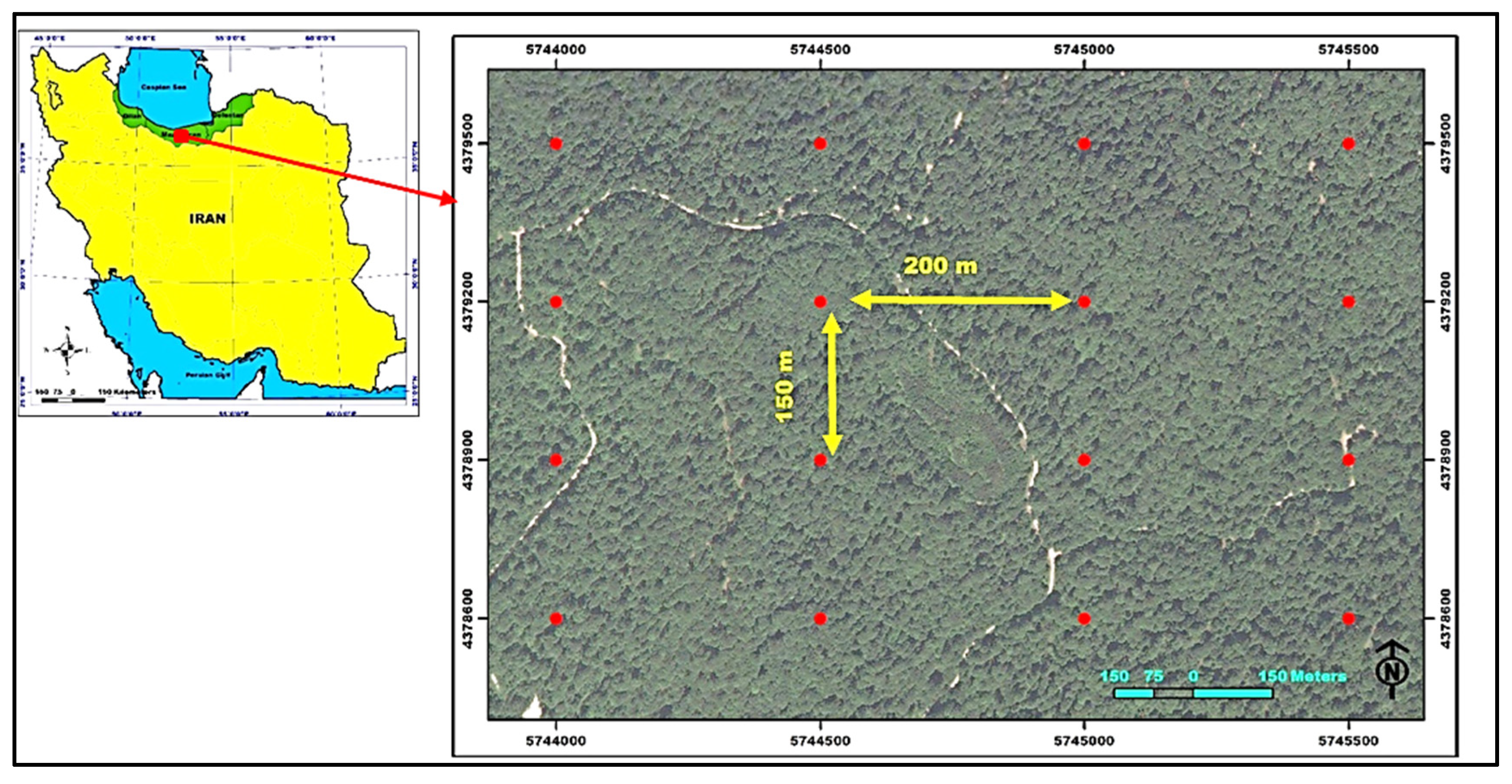
Hyrcanian forests are of great importance as the only commercial forests in Iran that have temperate broad-leaved species. Their approximate area is 1.85 million hectares and about 15% of Iran’s forests. This region is of special importance with about 44% of the vascular plants in Iran. There are about 500 species of plants native to Iran in these forests. Therefore, sustainable and effective planning and management in this region have always been a major concern. Accurate estimation of the characteristics of these forests, including diameter increment, has great importance for planners [30].
However, the application of ANNs and the ANFIS to predict the diameter increment in uneven-aged forests has not been previously conducted in the world. Therefore, by providing diameter increment models in mixed and uneven-aged Caspian forests using these two techniques, we are presenting here an account of novel approaches to build a foundation for future studies.
Therefore, in this study, some specific issues were investigated: (1) estimation of the diameter increment in mixed and uneven-aged forests using machine learning (the main objective), (2) the potential use of nonparametric models including ANNs and the ANFIS for the estimation of the diameter increment, (3) a comparison between the ANFIS and ANN in estimating tree increment, and finally (4) optimization of ANN and ANFIS methods when used in predicting tree diameter increment.

2. Materials and Methods

2.1. Study Area and Data

Kheyroud educational research forest is located in watershed 45 in northern forests of Iran seven kilometers east of the city of Noshahr in Mazandaran Province. The forest plan categorizes this area into eight districts including the Gorazbon district. The Gorazbon district, with an area of 934.24 hectares, is the third largest district of Kheyroud forest (Figure 1). This district is located in the longitudinal range 51° 36′ 30″ to 51° 39′ 30″ and latitude 36° 32′ 0″ to 36° 34′ 0″. The general orientation of this district is north–south, and the minimum and maximum altitudes are 840 and 1350 m above sea level. Brown soil is typical in this district.
The data used in modeling were obtained from two sampling periods (2003 and 2012) with fixed-area sample plots. In 2003, using a 150 × 200 m grid, 256 permanent circular sample plots with area of 0.1ha were present in the Gorazbon district in the form of a systematic sample. Each sample plot was recorded with a GNSS receiver. The accuracy of the registration of the forest monitoring permanent sample plots’ center depends on several factors, including the density of the canopy of the study forest [31]. Inside the sample plots, the diameter at breast height (DBH) of all living trees with a diameter of more than 7.5 cm was measured using caliper, and their values were recorded in inventory forms and in one-centimeter classes. These operations were repeated after nine years. In total, seven tree species consisting of Fagus orientalis, Carpinus betulus, Quercus castaneifolia, Alnus subcordat, Acer cappadocicum, Acer velutinum, and Tilia begonifolia were tallied in sample plots. For the sake of our study and simplification, we put these species into four broad groups such as beech, hornbeam, chestnut-leaved oak, and other species [32].

2.2. Determination of the Model Inputs

The data we recorded were used as input to calculate models (Table 1). These inputs consisted of natural logarithm of DBH (cm), square of DBH (cm2), basal area of the largest tree (BAL) (m2/ha), Shannon–Weiner’s species diversity index (HS) (Equation (1)) [33], size diversity index (Hd) (Equation (2)), and the mean of basal area (BA) in sample plot (m2) (Table 2).
H s = i = 1 n s B i B ln ( B i B )
H d = j = 1 n d B j B ln ( B j B )

2.3. Model Development

Almost 80% of the studied trees come from two species (beech and hornbeam), and nearly 20% fall into chestnut-leaved oak and other species groups in the study site. Consequently, the species were divided into four groups of beech (2215 trees), hornbeam (3131 trees), chestnut-leaved oak (340 trees), and other species (856 trees), and a separate model was developed for each group.
Machine learning has various algorithms including artificial neural network (ANN), genetic algorithm, fuzzy logic, and neuro-fuzzy [30,34,35]. For predicting the diameter increment of individual trees, two techniques of adaptive neuro-fuzzy inference system (ANFIS) and multi-layer perceptron (MLP) neural network were designed and implemented in MATLAB software version 2016. Prior to delving into the details of these techniques, it is better to describe the data stratification method. In general, the data used in the ANN model were divided into two subsets of training and testing data. Training section is larger and usually involves 70 to 80% of the data and is used for training the learning patterns to the network [36,37]. The test section is not utilized in the network learning process. Rather, it is used for comparing different models in terms of network power (goodness of fit) and generalization [38]. In the present study, the k-fold cross validation method was utilized. This method has been applied by Kozak and Kozak [39] and others. In our study, all observations after random distribution were divided into four-fold (i.e., k = 4), and for each species group every data set contained 25% of observations. Therefore, four data sets were created with different structures (Table 3). The data sets were utilized to construct four models for both MLP and ANFIS techniques. The three sets of data were used for model development (training) and one data set for error estimation in each model. For each species group, 4 models with different formation of the data sets were obtained. The final step included averaging the calculations of outputs of the four models.

2.3.1. Multilayer Perceptron Artificial Neural Network (MLP)

The typical architecture of MLP consists of three layers: an input, hidden, and output layer [40]. The architecture of these networks includes the number of layers, the number of neurons, the transfer function of each neuron, and how the layers are interconnected depending on the type of problem [26]. The number of independent variables of the problem determines the number of network inputs, and the number of dependent variables specifies the neurons’ number of output layer. The main issue in the design of the ANN is the determination of the number of suitable neurons in the hidden layer(s), which is achieved with the trial-and-error method. A single neuron is not very useful for modeling real and complex systems, whereas several neurons have a high power when they are linked with one or more layers. In general, the larger number of layers enables the system to represent more complexities. However, on the other hand, a high number of layers decreases the accuracy of the prediction model and may prevent the network from converging. In such a case, it has been proven that MLPs with one hidden layer, a sigmoid function (in the hidden layer), and a linear function in the output layer are able to provide an approximation of all the functions, provided that there are enough neurons in the hidden layer [41,42]. Hence, in this study, the number of neurons in each layer was determined as follows:
(i)
The number of neurons in input layer: The determination of inputs number for each species group was obtained by trial and error. Thus, the combination with the lowest mean squared error (MSE) values was selected as the final combination of the model. The tested combinations are shown in Table 4. Therefore, according to each species group, the suitable and normalized inputs were entered into the network. Then, these inputs, using hyperbolic tangent (tansig) function [26], were passed from hidden layer to the output layer.
(ii)
The number of neurons in hidden layer: In MLP, the nodes of hidden layer are a structural sensitive parameter. This means that very low nodes could lead to ill training and high nodes lead to over-fitting [40]. In this study, the structures of MLP with 1 to 30 neurons in the hidden layer were analyzed and their prediction accuracy was evaluated.
(iii)
The number of neurons in output layer: According to the aim of this study (diameter increment estimation) and number of parameters, the neuron’s number in the output layer is equal to 1. The outputs of hidden layer are eventually passed through the output layer with a linear transfer function (purelin) to provide the final output of the model.
Table 4. Combinations of model inputs.
No.Model Inputs
1Natural logarithm of DBH (cm), square of DBH (m), BAL
2Natural logarithm of DBH (cm), square of DBH (m), BAL, the average of BA at sample plot
3Natural logarithm of DBH (cm), square of DBH (m), BAL, Hs
4Natural logarithm of DBH (cm), square of DBH (m), BAL, Hd
5Natural logarithm of DBH (cm), square of DBH (m), BAL, average BA at sample plot, Hs
6Natural logarithm of DBH (cm), square of DBH (m), BAL, average BA at sample plot, Hd
7Natural logarithm of DBH (cm), square of DBH (m), BAL, Hs, Hd
8Natural logarithm of DBH (cm), square of DBH (m), BAL, average BA at sample plot, Hs, Hd
The outputs of the model were compared with the target values, and the differences were calculated as suggested by earlier studies [43,44]. The process was continued until network’s weights were optimized. The prediction capability and performance of the developed ANN were determined using mathematical and statistical methods. In order to assess the network performance and terminate the training, the MSE was utilized as a measure of the accuracy of the ANN results. The Levenberg–Marquardt (LM) algorithm depicted the best performance in fitting functions. Therefore, this LM algorithm was used in this study.

2.3.2. Neuro-Fuzzy Inference System (ANFIS)

ANFIS was also used to predict diameter increment of individual trees. ANFIS structure consists of five layers: input nodes, rule nodes, average nodes, consequent nodes, and output nodes [45,46]. Each node has a function with an adjustable or fixed component [46]. The proper structure of the ANFIS is selected according to the input data, membership degree, the rules, and the membership functions of the input and output. The input values could become closer to the actual ones, if the membership degree components are adjusted during the training stage.
For our study, we used the same stratification method as was conducted for MLP (Table 4) during modeling and testing stages. Just as with MLP (Table 4), the inputs of ANFIS technique were determined by trial and error. ANFIS uses neural network learning algorithms and fuzzy logic to design nonlinear mapping between input and output space [22]. It also has the advantage of adaptation capability and rapid learning capacity [47]. In addition, it can adjust the conversion of human intelligence to fuzzy systems. The learning rule is based on the back-propagation algorithm with the aim of minimizing the MSE between the network output and the actual output. There are three types of systems included in the fuzzy inference system (FIS): Mamdani system, Sugeno system, and Tsukamoto system. In most cases, Mamdani system is used; however, the Sugeno system performs better than the former in computing and has a definite (crisp) output [46]. Therefore, for our study, modeling was performed by ANFIS technique using Sugeno system. The grid partitioning method was used to determine the degree and type of desirable membership functions such as triangular-shaped, trapezoidal-shaped, bell-shaped, Gaussian, pi-shaped, Gaussian 2, and sigmoid through trial and error. Further, the hybrid algorithm, which is a combination of the back-propagation algorithm and the least-squares error method, was used for training and adapting with the FIS.

2.3.3. Model Evaluation

Model evaluation is an important part of the modeling process and should be considered at different stages of modeling, including design, adjustment, and implementation. The evaluation of the model consists of two main stages, which include verification (qualitative) and validation (quantitative) [48]. In this study, five criteria including coefficient of determination (R2) (Equation (3)), root mean square error (RMSE) (Equation (4)), Akaike information criterion (AIC) (Equation (5)), Bayesian information criterion (BIC) (Equation (6)), and correlation coefficient (r) were used. The coefficient of determination (R2) is the proportion of the variance in the dependent variable that can be explained by the independent variables [49,50]. The root mean square error (RMSE) is the standard deviation of the residuals, which is the difference between the surveyed data and the fitted model [51,52].
R 2 = ( i = 1 N ( O i O ¯ ) ( P i P ¯ ) ) 2 i = 1 N ( O i O ¯ ) 2 i = 1 N ( P i P ¯ ) 2
RMSE = [ N 1 i = 1 N ( P i O i ) 2 ] 0.5
Akaike [53] proposed the Akaike information criterion (AIC) to estimate the expected Kullback–Leibler distance between the model generating the data and the fitted candidate model. AIC can be expressed as:
AIC = N . ln ( S S E ) + 2 n p a r
In order to overcome the over-estimation problem of AIC, Schwarz [54] proposed the Bayesian information criterion (BIC). BIC was derived using a Bayesian perspective, and it selects the model with the maximum posterior probability for a given prior probability. BIC can be expressed as:
BIC = N . ln ( S S E ) + n p a r ln ( N )
where O, p, O ¯ , P ¯ , N, npar, and SSE are observed values, estimated values, the average of observed values, the average of estimated values, total number of observations, number of inputs used in the model, and sum of the squared error (SSE), respectively. The best model has the highest value of R2 and the lowest of three other criteria (RMSE, AIC, and BIC).

3. Results

For the development of the ANN and ANFIS models, all networks examined in the MATLAB software environment (version 2016) were designed and implemented, and the results were derived separately for the groups of beech, hornbeam, chestnut-leaved oak, and other species. During the simulation process, the settings of the networks’ parameters were selected for both techniques (ANN and ANFIS) based on the minimum MSE via a trial-and-error procedure. The results indicated that for all groups of species in all data sets, the training of the network is more successful and has a higher accuracy (R2 and Pearson correlation coefficient (r)) than the network validation. In addition, the correlation values of the two techniques (ANN and ANFIS) for all species groups in all data sets were significant at a 0.01 level. The best combination of input variables was the same for both techniques (Table 5).
In the ANFIS technique, the k-fold strategy was used just as with the MLP. The results of this technique are presented separately for the four groups. The optimal ANFIS models were obtained by implementing a hybrid learning algorithm. The type and number of membership functions (in the form of trial and error) were determined using MSE criteria. The number of membership functions for all models was considered to be two, because the network was over-fitted with the increase in the number of membership functions. Moreover, triangular membership function was obtained as the best membership function. We used a linear transfer function in the output layer. The grid partitioning function was used to create the network architecture and the FIS. The number of iterations for optimization of the model was 100.

3.1. Beech Group

In the MLP model, data set D showed the best results in terms of the correlation and coefficient of determination (R2). However, by comparing the four data sets in terms of the three evaluation criteria of RMSE, AIC, and BIC, a different result is obtained, so that the lowest RMSE of training and validation were seen in groups C and B, respectively. Further, group C had the least value of AIC and BIC criteria and showed better performance (Table 6).
In the ANFIS model, given the R2 of both validation and training, data set C provided the best results. Moreover, by comparing four data sets in terms of the three evaluation criteria of RMSE, AIC, and BIC, data set C had the lowest value and presented the best result and performance (Table 6).
The error rates in the correlation and RMSE (MLP model) for the training and validation (four data sets) from the beech species are presented in Figure 2. The results of the models showed that for different data sets, correlation and RMSE values varied with increasing number of nodes, so that by increasing the number of nodes, the correlation value of the training of all data sets increases, while, for the validation data set, the trend is approximately unchanged. This trend is also seen in the case of RMSE criteria. The lowest correlation with two nodes and the highest correlation with 30 nodes were observed (Figure 2). Finally, according to the evaluation criteria of training and validation, it can be said that the best MLP network had 21 hidden nodes (i.e., a 5-21-1 structure).

3.2. Hornbeam Group

In the MLP model of the hornbeam group, data set B had the highest R2, data set A and C had the lowest RMSE, and data set B had the lowest AIC and BIC. Therefore, data set B generally gives the best result. In the ANFIS model, data set B had the highest R2, and C had the lowest RMSE, AIC, and BIC. Thus, for the hornbeam species, data set B generally provides the best outcome (Table 7).
The results of the MLP model for hornbeam species indicated that by increasing the number of nodes, the error rates in the correlation of training and validation data were incremental and decreasing, respectively. However, in the case of RMSE criteria, this trend is reversed. The lowest correlation was observed with two nodes and the highest correlation occurred with 29 nodes (Figure 3). According to the description provided, the best MLP model for hornbeam species consists of 29 hidden nodes (i.e., a 5-29-1 structure).

3.3. Chestnut-Leaved Oak Group

In the MLP model of this species, the difference between correlation and RMSE of training and validation is more than other studied species. The R2 of the training was approximately twice the R2 of the validation data. In both MLP and ANFIS models, in terms of correlation, RMSE, BIC, and AIC, it can be said that the data sets of A, B, B, and B provide the best results, respectively. Additionally, data set B also had the best performance in both models (Table 8).
The results of the changes in correlation and RMSE of chestnut-leaved oak species are slightly more complicated and do not show a tangible trend. It can only be said that by increasing the number of nodes, the value of correlation for training and validation data increases and decreases, respectively. The lowest correlation was observed with two nodes and the highest correlation with 21 nodes (Figure 4). The best MLP network of chestnut-leaved oak species has 21 hidden nodes (i.e., a 4-21-1 structure).

3.4. Other Species Group

In the MLP model of this group, the data set B had the highest R2 in training. For the other three evaluation criteria (RMSE, AIC, and BIC), the best performance was for the data set D. Finally, we can say that data set D provides the best performance because the validation provides better R2 than the training (Table 9). In the ANFIS model, data set C presented the best result in terms of all evaluation criteria (Table 9).
The results of the MLP model for the other species group showed that by increasing nodes (up to 25 nodes), the correlation showed an increasing trend. This means that by increasing the nodes, the error rate of the model decreases. The lowest correlation was found with one node (Figure 5). Therefore, the best MLP model of the other species group consists of 25 hidden nodes (i.e., a 4-25-1 structure).

4. Discussion

Since the habitat conditions of the Hyrcanian forests change from west to east and in elevation, it is very difficult to develop increment models. Therefore, identifying the appropriate predictors (inputs of the model) on increment and incorporating them into increment models is key to making predictions. For this purpose, the best input variables in the diameter increment models of four groups of beech, hornbeam, chestnut-leaved oak, and other species were identified using MLP (a class of feedforward ANN) and ANFIS techniques. The results were then compared.
Our results indicated that in relation to each group of species, different parameters could be significant, such as a previous study concluded [55,56]. For example, in relation to beech species, factors such as DBH and natural logarithm of DBH, BAL, Hd, and average of BA were significant. These variables are associated with hornbeam (DBH, natural logarithm of DBH, and BAL) and chestnut-leaved oak, and other species (DBH and natural logarithm of DBH, BAL, and Hs) showed a different pattern. The effectiveness of the two indices, size diversity and species diversity of Shannon–Wiener, on the increment rate were consistent with the results of Liang [57]. In the research for oak forests, an individual-tree model was presented, and it was concluded that the indices affecting the diameter increment include tree size, basal area, tree diameter, volume inventory, and site index [58]. The results of Lhotka and Loewenstein [59] on the development of individual-tree diameter growth models for the Missouri forest stands in the United States showed that the BAL parameter was effective for all species, while the patterns of remaining predictors were different for other species. The results of Lhotka and Loewenstein [59] were in line with the findings of the present study, except in one case. Unlike their findings, in our study the species composition (species diversity index) was not effective for all species groups. In general, the BAL variable has been used as the most important competition variable in previous growth and increment modeling studies (e.g., [60,61,62,63,64]). In this study, we incorporated all the measured independent variables, i.e., DBH, BAL, HS, Hd, BA, number of trees per hectare, slope, aspect, and altitude into the modeling process. However, only DBH, BAL, BA, HS, and Hd were significant and considered in the final model. Other variables were removed from the final model because they were insignificant in terms of correlation because the study area was relatively consistent in some respects (e.g., slope). If a larger area is selected for study, these variables may become meaningful [30,40]. However, variables of size diversity and species diversity have not been closely evaluated, except for few studies (e.g., [1,57]). Given the fact that the Hyrcanian forests have high biodiversity (species diversity) and high size diversity [30], consideration of these two indices in new studies is most important.
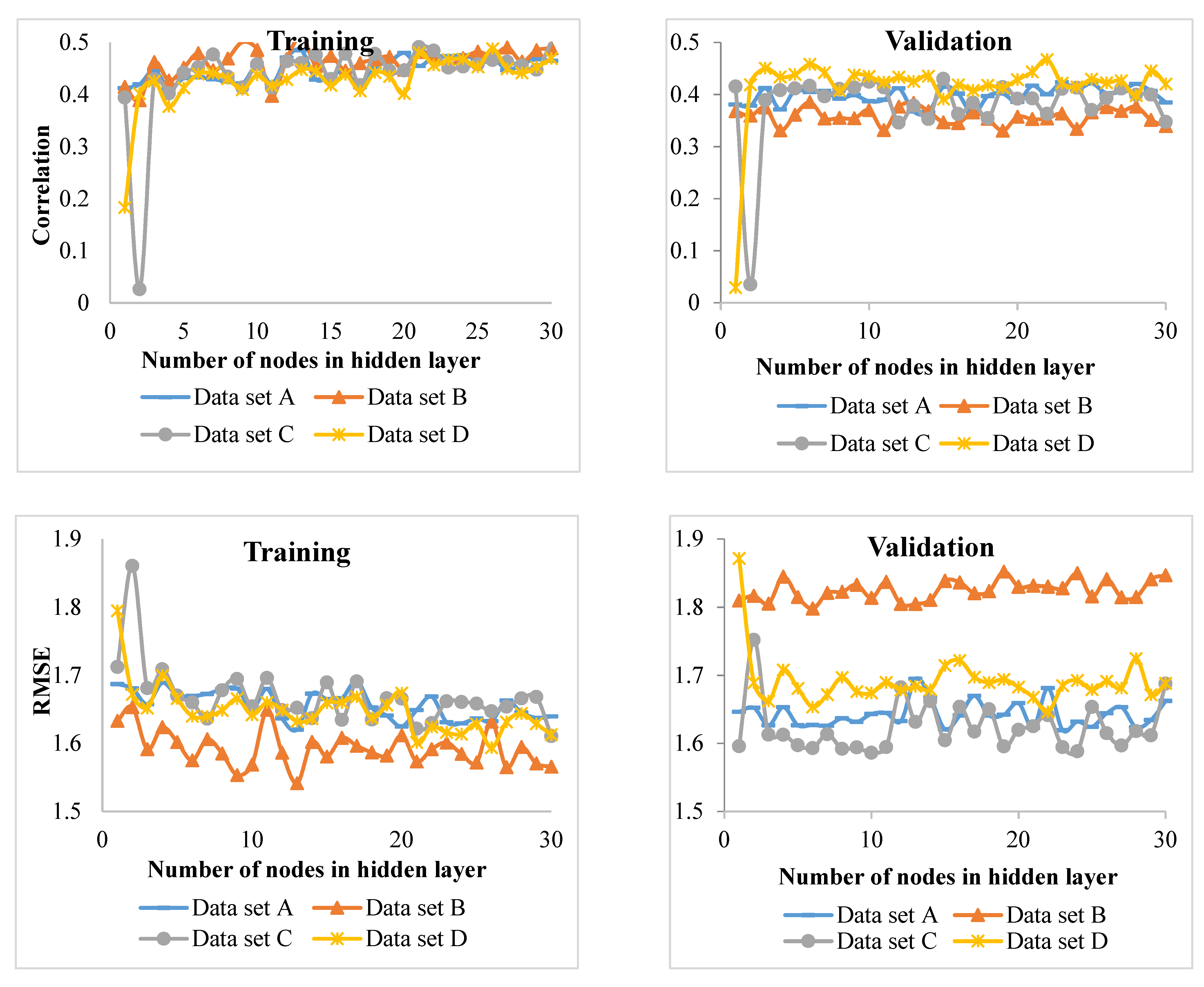
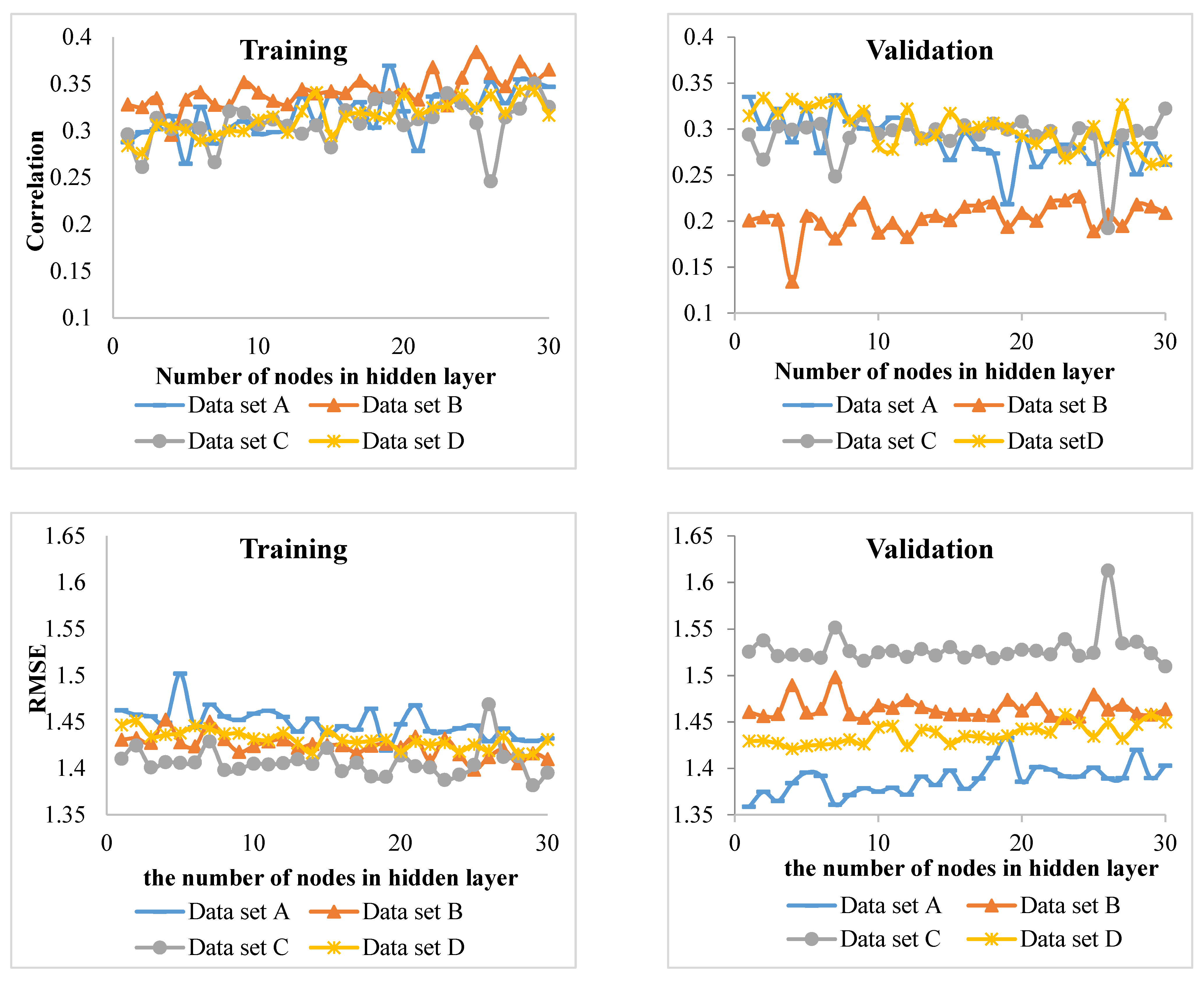
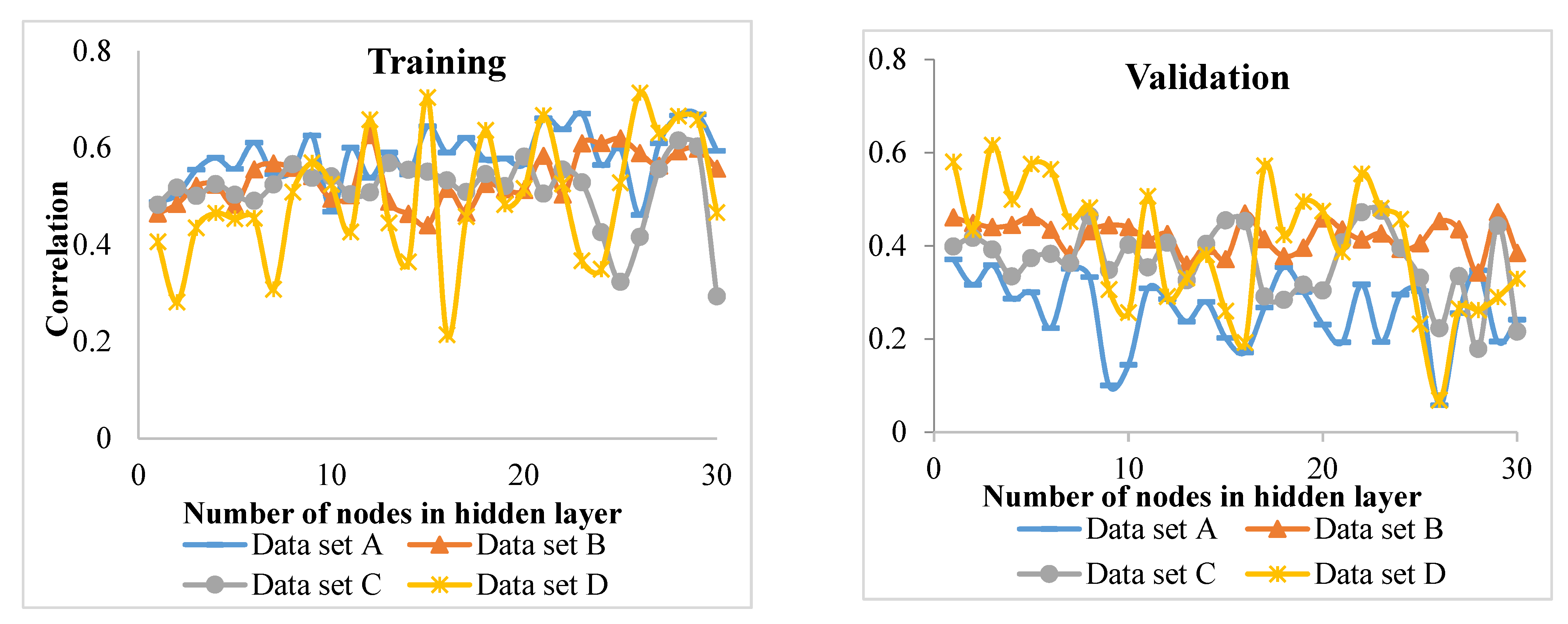
Comparison of the MLP and ANFIS techniques showed that the latter performed better for of the beech and chestnut-leaved oak groups. On the other hand, MLP showed promising results for the hornbeam and other species groups. However, in the study of Vieira et al. [18], no significant difference was observed for diameter growth estimation between the ANFIS and ANN techniques. It seems that with increasing complexity of the relationship, the ANN technique brings better results [65]. Beech and chestnut-leaved oak clusters occupy more distinctive site conditions than the other two groups in the Hyrcanian forests. For instance, the beech class is mainly situated in the northern side [6], while the chestnut-leaved oak group is situated in the southern and southwestern directions. The hornbeam group appeared in almost all sample plots (high distribution). Therefore, the determination of its diameter increment was more challenging and complicated, and the coefficient of determination (R2) of the model showed the lowest value compared to the other tree groups. This means that the inputs of the model did not properly account for the variation in the diameter increment. It is recommended that hybrid models be fitted for this group. The low R2 values can be attributed to a large number of heterogeneous data used in this study. However, the values were statistically significant and allowed for identifying major growth driving factors. For future works, other factors (e.g., soil properties) from a large-scale area might be incorporated into the models for measuring, and perhaps improving, their performance.
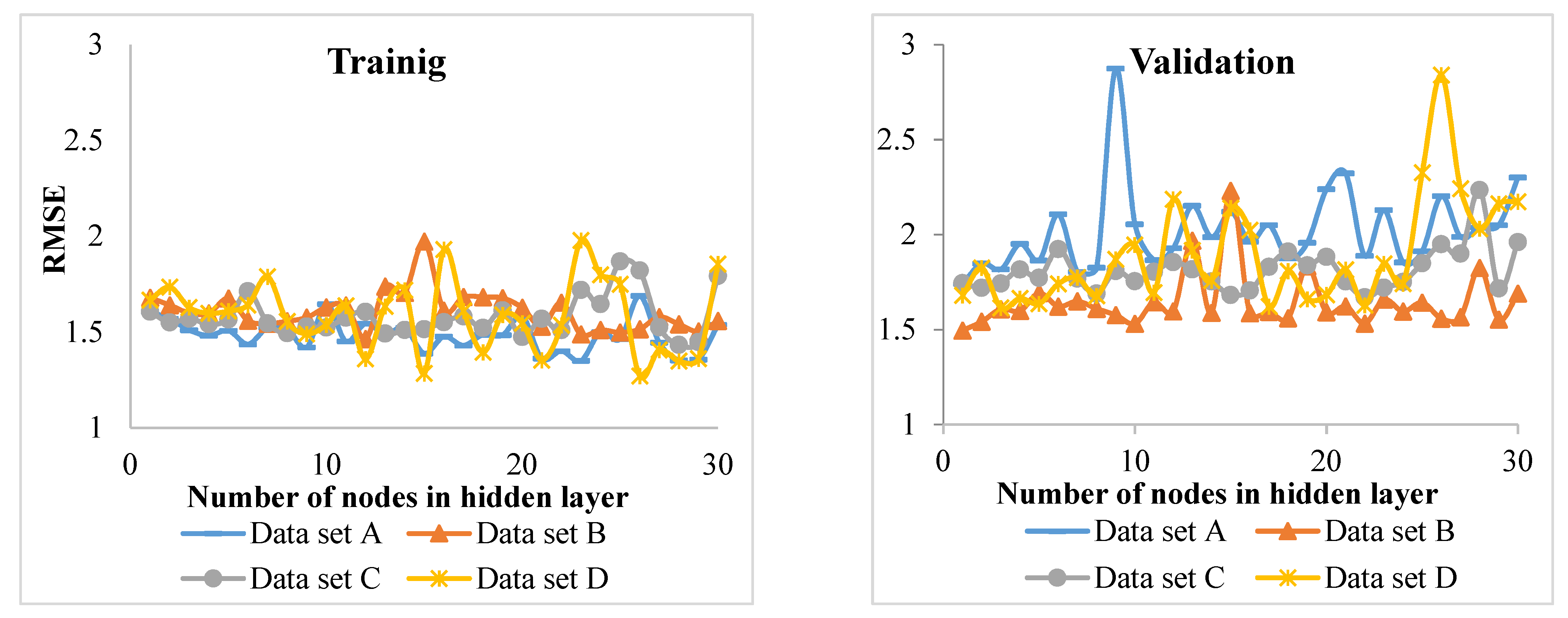
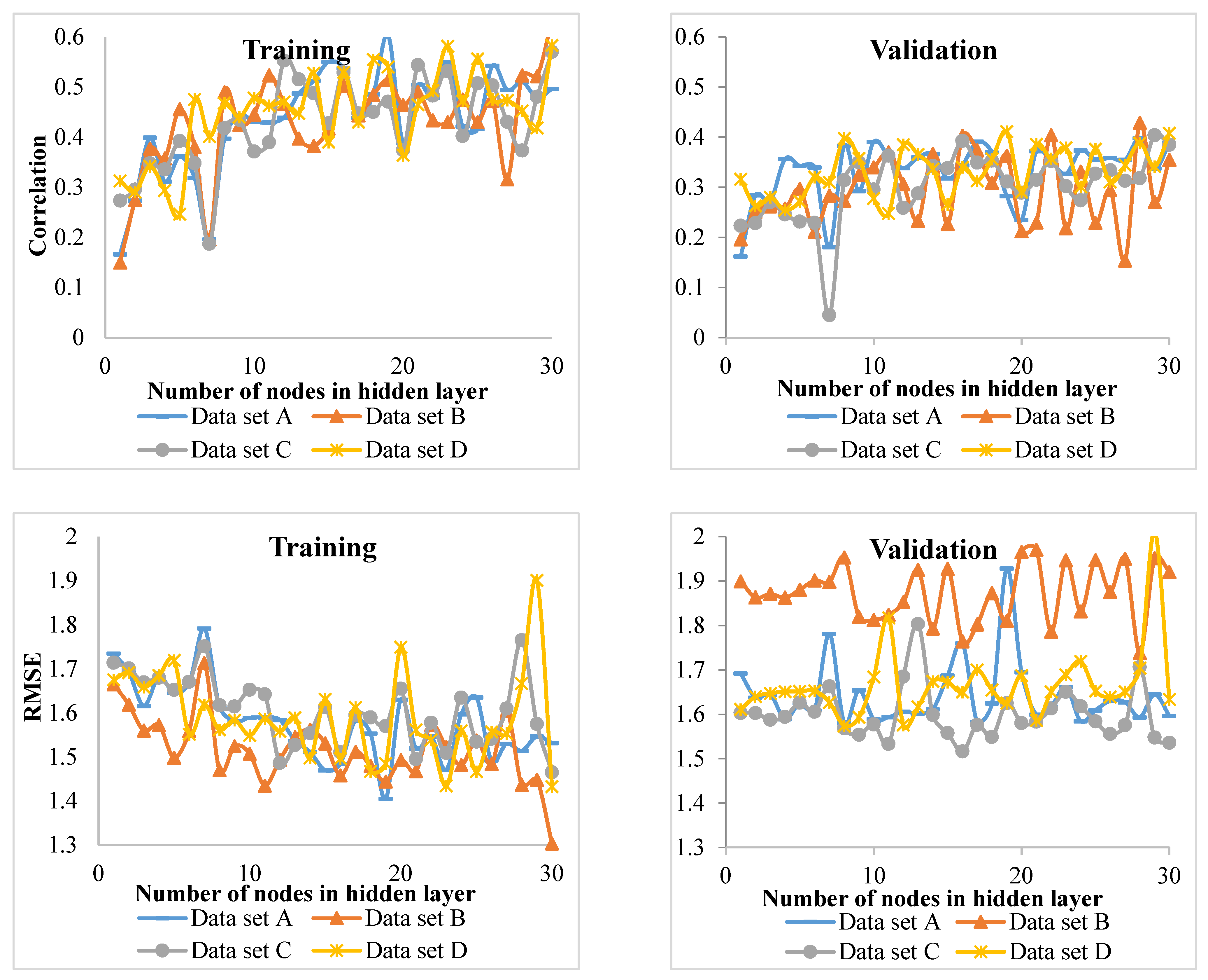
Using the k-fold strategy in evaluation showed that different combinations of data give different results. Therefore, the use of this strategy and the acquisition of the final model of the four-folds (where, k = 4) average provides the most realistic result. We found this strategy useful, as it has been considered promising in other recent studies (e.g., [26,61,63]). The correlation coefficient of models, despite not having high values, were significant at a 0.01 level. There could be several reasons for such a pattern of correlation coefficients. One possibility could be the existence of trees with the same diameter and significant differences in diameter increment values [66], which resulted from forest competition and succession [67]. The second reason might be the autocorrelation of data used in increment models due to both time and spatial components [26]. Although permanent sample plots are the most popular method for estimating forest growth and yield and have been used in numerous studies (e.g., [60,61,62,63]), they are not immune from the autocorrelation. The autocorrelation created within the sample plots was greater than the autocorrelation between the sample plots, because the sample plots are separated by more distance than the trees within a sample plot [26].
Since previous studies carried out using ANNs and the ANFIS are different from our study in terms of diverse aspects such as forest type (even-aged or uneven-aged) and research goal (diameter increment, diameter growth, basal area growth survival, etc.), comparisons between our results and those of most prior studies are not possible.

5. Conclusions

The aim of this study was to provide insight into the utilization of two machine learning methods (MLP and ANFIS) for developing a diameter increment model for the Hyrcanian forests. The findings of this study would for the first time provide general information on the number of optimal hidden neurons (in ANNs) and the type and number of membership functions (in ANFIS) for diameter increment modeling.
RMSE and R2 of the MLP and ANFIS models were estimated for the four groups of beech ((1.61 and 0.23) and (1.57 and 0.26)), hornbeam ((1.42 and 0.13) and (1.49 and 0.10)), chestnut-leaved oak ((1.55 and 0.28) and (1.47 and 0.39)), and other species ((1.44 and 0.32) and (1.5 and 0.24)), respectively. Despite the low coefficient of determination, the correlation test in both techniques was significant at a 0.01 level for all four groups. In general, the ANFIS worked better when the data from the oak and beech groups were used, probably because these groups represent the dense-covered areas with trees. On the other hand, the ANN performed better with the hornbeam and other species groups that represent a wide but less-covered area with trees. Our study also provides information on optimizing and adjusting the parameters necessary for the application of machine learning in developing prediction models for the estimation of the diameter increment in the Hyrcanian forests. We found that modeling techniques have a deep relationship with the nature of the tree species. The results provide guidance for future studies in the same area (Hyrcanian forest) or elsewhere in the diverse forests of the world.

Author Contributions

Conceptualization: A.S. and M.B.; data collection: A.S., M.B. and B.K.; formal analysis: A.S., M.B., B.K., M.N. and M.O.; validation: A.S., M.B., B.K., M.N., H.U.M.A. and M.O.; supervision: M.B. and M.N.; writing—original draft: all authors; funding acquisition: N.A.-A. and A.J. All authors have read and agreed to the published version of the manuscript.

Funding

This research received no external funding.

Institutional Review Board Statement

Not applicable.

Informed Consent Statement

Not applicable.

Data Availability Statement

The data presented in this study will be available on interested request from the corresponding author.

Acknowledgments

We thank Harold Burkhart from Virginia Polytechnic Institute and State University and three anonymous reviewers for their helpful comments on an earlier draft of this paper.

Conflicts of Interest

The authors declare no conflict of interest.

References

  1. Wang, W.; Chen, X.; Zeng, W.; Wang, J.; Meng, J. Development of a mixed-effects individual-tree basal area increment model for oaks (Quercus spp.) considering forest structural diversity. Forests 2019, 10, 474. [Google Scholar] [CrossRef] [Green Version]
  2. Bombrun, M.; Dash, J.P.; Pont, D.; Watt, M.S.; Pearse, G.D.; Dungey, H.S. Forest-scale phenotyping: Productivity characterisation through machine learning. Front. Plant Sci. 2020, 11, 99. [Google Scholar] [CrossRef] [PubMed]
  3. Burkhart, H.E.; Tomé, M. Modeling Forest Trees and Stands; Springer Science & Business Media: Dordrecht, Germany, 2012. [Google Scholar]
  4. Burkhart, H.; Brooks, T. Status and future of growth and yield models. In Proceedings of the State-of-the-Art Methodology of Forest Inventory: A Symposium Proceedings, Syracuse, NY, USA, 30 July–5 August 1990; pp. 409–414. [Google Scholar]
  5. Bayat, M.; Pukkala, T.; Namiranian, M.; Zobeiri, M. Productivity and optimal management of the uneven-aged hardwood forests of Hyrcania. Eur. J. For. Res. 2013, 132, 851–864. [Google Scholar] [CrossRef]
  6. Bourque, C.P.-A.; Bayat, M.; Zhang, C. An assessment of height–diameter growth variation in an unmanaged Fagus orientalis-dominated forest. Eur. J. For. Res. 2019, 138, 607–621. [Google Scholar] [CrossRef]
  7. Burkhart, H.E. Modelling growth and yield for intensively managed forests. J. For. Environ. Sci. 2008, 24, 119–126. [Google Scholar]
  8. He, S.; Guo, F.; Zou, Q. MRMD 2.0: A python tool for machine learning with feature ranking and reduction. Curr. Bioinform. 2020, 15, 1213–1221. [Google Scholar] [CrossRef]
  9. Cai, J. Ship electronic information identification technology based on machine learning. J. Coast. Res. 2020, 103, 770–774. [Google Scholar] [CrossRef]
  10. Mehtätalo, L.; Lappi, J. Biometry for Forestry and Environmental Data: With Examples in R.; CRC Press: Boca Raton, FL, USA, 2020. [Google Scholar]
  11. Ou, Q.; Lei, X.; Shen, C. Individual tree diameter growth models of larch–spruce–fir mixed forests based on machine learning algorithms. Forests 2019, 10, 187. [Google Scholar] [CrossRef] [Green Version]
  12. de Silva, R.M.; Brandão, F.G.; Baleeiro, G.B.; Valentim, F.L.; de Mendonça, A.R.; Pires, D.M. Fuzzy and neuro-fuzzy estimates of the total height of eucalyptus trees. In Proceedings of the 2008 ACM Symposium on Applied Computing, Fortaleza, Brazil, 16–20 May 2008; pp. 1772–1776. [Google Scholar]
  13. Özçelik, R.; Diamantopoulou, M.J.; Brooks, J.R.; Wiant Jr, H.V. Estimating tree bole volume using artificial neural network models for four species in Turkey. J. Environ. Manag. 2010, 91, 742–753. [Google Scholar] [CrossRef] [PubMed]
  14. Soares, F.A.A.; Flôres, E.L.; Cabacinha, C.D.; Carrijo, G.A.; Veiga, A.C.P. Recursive diameter prediction and volume calculation of eucalyptus trees using Multilayer Perceptron Networks. Comput. Electron. Agric. 2011, 78, 19–27. [Google Scholar] [CrossRef]
  15. Bayat, M.; Bettinger, P.; Heidari, S.; Henareh Khalyani, A.; Jourgholami, M.; Hamidi, S.K. Estimation of tree heights in an uneven-aged, mixed forest in northern Iran using artificial intelligence and empirical models. Forests 2020, 11, 324. [Google Scholar] [CrossRef] [Green Version]
  16. Miao, R.; Liu, Y.; Wu, L.; Wang, D.; Liu, Y.; Miao, Y.; Yang, Z.; Guo, M.; Ma, J. Effects of long-term grazing exclusion on plant and soil properties vary with position in dune systems in the Horqin Sandy Land. Catena 2022, 209, 105860. [Google Scholar] [CrossRef]
  17. Li, X.; Zhang, K.; Gu, P.; Feng, H.; Yin, Y.; Chen, W.; Cheng, B. Changes in precipitation extremes in the Yangtze River Basin during 1960–2019 and the association with global warming, ENSO, and local effects. Sci. Total Environ. 2021, 760, 144244. [Google Scholar] [CrossRef] [PubMed]
  18. Vieira, G.C.; de Mendonça, A.R.; da Silva, G.F.; Zanetti, S.S.; da Silva, M.M.; Dos Santos, A.R. Prognoses of diameter and height of trees of eucalyptus using artificial intelligence. Sci. Total Environ. 2018, 619, 1473–1481. [Google Scholar] [CrossRef]
  19. Chen, J.; Yang, H.; Man, R.; Wang, W.; Sharma, M.; Peng, C.; Parton, J.; Zhu, H.; Deng, Z. Using machine learning to synthesize spatiotemporal data for modelling DBH-height and DBH-height-age relationships in boreal forests. For. Ecol. Manag. 2020, 466, 118104. [Google Scholar] [CrossRef]
  20. Wijayanto, A.K.; Sani, O.; Kartika, N.D.; Herdiyeni, Y. Classification model for forest fire hotspot occurrences prediction using ANFIS algorithm. IOP Conf. Ser. Earth Environ. Sci. 2017, 54, 012059. [Google Scholar] [CrossRef]
  21. Guan, B.T.; Gertner, G. Modeling red pine tree survival with an artificial neural network. For. Sci. 1991, 37, 1429–1440. [Google Scholar]
  22. Jang, J.-S. ANFIS: Adaptive-network-based fuzzy inference system. IEEE Trans. Syst. Man Cybern. 1993, 23, 665–685. [Google Scholar] [CrossRef]
  23. Karaboga, D.; Kaya, E. Adaptive network based fuzzy inference system (ANFIS) training approaches: A comprehensive survey. Artif. Intell. Rev. 2019, 52, 2263–2293. [Google Scholar] [CrossRef]
  24. Reis, L.P.; de Souza, A.L.; dos Reis, P.C.M.; Mazzei, L.; Soares, C.P.B.; Torres, C.M.M.E.; da Silva, L.F.; Ruschel, A.R.; Rêgo, L.J.S.; Leite, H.G. Estimation of mortality and survival of individual trees after harvesting wood using artificial neural networks in the amazon rain forest. Ecol. Eng. 2018, 112, 140–147. [Google Scholar] [CrossRef]
  25. Reis, L.P.; de Souza, A.L.; Mazzei, L.; dos Reis, P.C.M.; Leite, H.G.; Soares, C.P.B.; Torres, C.M.M.E.; da Silva, L.F.; Ruschel, A.R. Prognosis on the diameter of individual trees on the eastern region of the amazon using artificial neural networks. For. Ecol. Manag. 2016, 382, 161–167. [Google Scholar] [CrossRef]
  26. Ashraf, M.I.; Zhao, Z.; Bourque, C.P.A.; MacLean, D.A.; Meng, F.-R. Integrating biophysical controls in forest growth and yield predictions with artificial intelligence technology. Can. J. For. Res. 2013, 43, 1162–1171. [Google Scholar] [CrossRef]
  27. Richards, M.; McDonald, A.J.S.; Aitkenhead, M. Optimisation of competition indices using simulated annealing and artificial neural networks. Ecol. Model. 2008, 214, 375–384. [Google Scholar] [CrossRef]
  28. Ashraf, M.I.; Meng, F.-R.; Bourque, C.P.-A.; MacLean, D.A. A novel modelling approach for predicting forest growth and yield under climate change. PLoS ONE 2015, 10, e0132066. [Google Scholar] [CrossRef] [PubMed] [Green Version]
  29. Castro, R.; Soares, C.; Leite, H.; Souza, A.; Martins, F.; Nogueira, G.; Romarco, M. Artificial neural networks effectiveness to estimate mortality in a Semi-Deciduous Seasonal Forest. Aust. J. Basic Appl. Sci. 2015, 9, 435–444. [Google Scholar]
  30. Bayat, M.; Bettinger, P.; Hassani, M.; Heidari, S. Ten-year estimation of Oriental beech (Fagus orientalis Lipsky) volume increment in natural forests: A comparison of an artificial neural networks model, multiple linear regression and actual increment. For. Int. J. For. Res. 2021, 94, 598–609. [Google Scholar] [CrossRef]
  31. Bettinger, P.; Merry, K.; Bayat, M.; Tomaštík, J. GNSS use in forestry–A multi-national survey from Iran, Slovakia and southern USA. Comput. Electron. Agric. 2019, 158, 369–383. [Google Scholar] [CrossRef]
  32. Bayat, M.; Namiranian, M.; Zobeiri, M. Volume, height and wood production modeling using the changes in a nine years rotation (case study: Gorazbon district in Kheyroud forest, north of Iran). For. Wood Prod. 2014, 67, 423–435. [Google Scholar]
  33. Fedor, P.; Zvaríková, M. Biodiversity indices. Encycl. Ecol. 2019, 2, 337–346. [Google Scholar]
  34. Chen, X.; Quan, Q.; Zhang, K.; Wei, J. Spatiotemporal characteristics and attribution of dry/wet conditions in the Weihe River Basin within a typical monsoon transition zone of East Asia over the recent 547 years. Environ. Model. Softw. 2021, 143, 105116. [Google Scholar] [CrossRef]
  35. Quan, Q.; Gao, S.; Shang, Y.; Wang, B. Assessment of the sustainability of Gymnocypris eckloni habitat under river damming in the source region of the Yellow River. Sci. Total Environ. 2021, 778, 146312. [Google Scholar] [CrossRef] [PubMed]
  36. Bayat, M.; Burkhart, H.; Namiranian, M.; Hamidi, S.K.; Heidari, S.; Hassani, M. Assessing Biotic and Abiotic Effects on Biodiversity Index Using Machine Learning. Forests 2021, 12, 461. [Google Scholar] [CrossRef]
  37. Xiong, Z.; Mo, F.; Zhao, X.; Xu, F.; Zhang, X.; Wu, Y. Dynamic Texture Classification Based on 3D ICA-Learned Filters and Fisher Vector Encoding in Big Data Environment. J. Signal Processing Syst. 2022, 1–15. [Google Scholar] [CrossRef]
  38. Hagan, M.T.; Demuth, H.B.; Beale, M. Neural Network Design; PWS Publishing Co.: Boston, MA, USA, 1997. [Google Scholar]
  39. Kozak, A.; Kozak, R. Does cross validation provide additional information in the evaluation of regression models? Can. J. For. Res. 2003, 33, 976–987. [Google Scholar] [CrossRef]
  40. Hamidi, S.K.; Weiskittel, A.; Bayat, M.; Fallah, A. Development of individual tree growth and yield model across multiple contrasting species using nonparametric and parametric methods in the Hyrcanian forests of northern Iran. Eur. J. For. Res. 2021, 140, 421–434. [Google Scholar] [CrossRef]
  41. Hecht-Nielsen, R. Kolmogorov’s mapping neural network existence theorem. In Proceedings of the International Conference on Neural Networks, San Diego, CA, USA, 21–24 June 1987; pp. 11–14. [Google Scholar]
  42. Liu, F.; Zhang, G.; Lu, J. Multisource heterogeneous unsupervised domain adaptation via fuzzy relation neural networks. IEEE Trans. Fuzzy Syst. 2020, 29, 3308–3322. [Google Scholar] [CrossRef]
  43. Lek, S.; Park, Y. Artificial neural networks. In Encyclopedia of Ecology, Five-Volume Set; Elsevier Inc.: Amsterdam, The Netherlands, 2008; pp. 237–245. [Google Scholar]
  44. Demuth, H.; Beale, M.; Hagan, M. Neural Network Toolbox; The MathWorks, Inc.: Natick, MA, USA, 1992. [Google Scholar]
  45. Chen, S.H.; Lin, Y.H.; Chang, L.C.; Chang, F.J. The strategy of building a flood forecast model by neuro-fuzzy network. Hydrol. Processes Int. J. 2006, 20, 1525–1540. [Google Scholar] [CrossRef]
  46. Kisi, O.; Haktanir, T.; Ardiclioglu, M.; Ozturk, O.; Yalcin, E.; Uludag, S. Adaptive neuro-fuzzy computing technique for suspended sediment estimation. Adv. Eng. Softw. 2009, 40, 438–444. [Google Scholar] [CrossRef]
  47. Şahin, M.; Erol, R. A comparative study of neural networks and ANFIS for forecasting attendance rate of soccer games. Math. Comput. Appl. 2017, 22, 43. [Google Scholar] [CrossRef] [Green Version]
  48. Oreskes, N.; Shrader-Frechette, K.; Belitz, K. Verification, validation, and confirmation of numerical models in the earth sciences. Science 1994, 263, 641–646. [Google Scholar] [CrossRef] [PubMed] [Green Version]
  49. Chicco, D.; Warrens, M.J.; Jurman, G. The coefficient of determination R-squared is more informative than SMAPE, MAE, MAPE, MSE and RMSE in regression analysis evaluation. PeerJ Comput. Sci. 2021, 7, e623. [Google Scholar] [CrossRef] [PubMed]
  50. Xu, H.; Wang, X.-Y.; Liu, C.-N.; Chen, J.-N.; Zhang, C. A 3D root system morphological and mechanical model based on L-Systems and its application to estimate the shear strength of root-soil composites. Soil Tillage Res. 2021, 212, 105074. [Google Scholar] [CrossRef]
  51. Hu, Y.; Xu, X.; Wu, F.; Sun, Z.; Xia, H.; Meng, Q.; Huang, W.; Zhou, H.; Gao, J.; Li, W. Estimating forest stock volume in Hunan Province, China, by integrating in situ plot data, Sentinel-2 images, and linear and machine learning regression models. Remote Sens. 2020, 12, 186. [Google Scholar] [CrossRef] [Green Version]
  52. Liang, X.; Lu, T.; Yishake, G. How to promote residents’ use of green space: An empirically grounded agent-based modeling approach. Urban For. Urban Green. 2022, 67, 127435. [Google Scholar] [CrossRef]
  53. Akaike, H. Information theory and an extension of the maximum likelihood principle. In Selected Papers of Hirotugu Akaike; Springer: Berlin/Heidelberg, Germany, 1998; pp. 199–213. [Google Scholar]
  54. Schwarz, G. Estimating the dimension of a model. Ann. Stat. 1978, 461–464. [Google Scholar] [CrossRef]
  55. Liang, J. Dynamics and management of Alaska boreal forest: An all-aged multi-species matrix growth model. For. Ecol. Manag. 2010, 260, 491–501. [Google Scholar] [CrossRef]
  56. Li, W.; Shi, Y.; Zhu, D.; Wang, W.; Liu, H.; Li, J.; Shi, N.; Ma, L.; Fu, S. Fine root biomass and morphology in a temperate forest are influenced more by the nitrogen treatment approach than the rate. Ecol. Indic. 2021, 130, 108031. [Google Scholar] [CrossRef]
  57. Liang, J.; Buongiorno, J.; Monserud, R.A.; Kruger, E.L.; Zhou, M. Effects of diversity of tree species and size on forest basal area growth, recruitment, and mortality. For. Ecol. Manag. 2007, 243, 116–127. [Google Scholar] [CrossRef]
  58. Lhotka, J.M. Examining growth relationships in Quercus stands: An application of individual-tree models developed from long-term thinning experiments. For. Ecol. Manag. 2017, 385, 65–77. [Google Scholar] [CrossRef]
  59. Lhotka, J.M.; Loewenstein, E.F. An individual-tree diameter growth model for managed uneven-aged oak-shortleaf pine stands in the Ozark Highlands of Missouri, USA. For. Ecol. Manag. 2011, 261, 770–778. [Google Scholar] [CrossRef]
  60. Tenzin, J.; Tenzin, K.; Hasenauer, H. Individual tree basal area increment models for broadleaved forests in Bhutan. For. Int. J. For. Res. 2017, 90, 367–380. [Google Scholar] [CrossRef]
  61. Dănescu, A.; Albrecht, A.T.; Bauhus, J.; Kohnle, U. Geocentric alternatives to site index for modeling tree increment in uneven-aged mixed stands. For. Ecol. Manag. 2017, 392, 1–12. [Google Scholar] [CrossRef]
  62. Roik, M.; Machado, S.d.A.; Figueiredo Filho, A.; Sanquetta, C.R.; Roveda, M.; Stepka, T.F. Diameter increment modeling in an Araucaria forest fragment using cluster analysis. Floresta E Ambiente 2018, 25, 3787–4033. [Google Scholar] [CrossRef]
  63. Riofrío, J.; del Río, M.; Maguire, D.A.; Bravo, F. Species mixing effects on height–diameter and basal area increment models for scots pine and maritime pine. Forests 2019, 10, 249. [Google Scholar] [CrossRef] [Green Version]
  64. Hess, A.F.; Minatti, M.; Costa, E.A.; Schorr, L.P.B.; da Rosa, G.T.; de Arruda Souza, I.; Borsoi, G.A.; Liesenberg, V.; Stepka, T.F.; Abatti, R. Height-to-diameter ratios with temporal and dendro/morphometric variables for Brazilian pine in south Brazil. J. For. Res. 2021, 32, 191–202. [Google Scholar] [CrossRef]
  65. Hamidi, S.K.; Zenner, E.K.; Bayat, M.; Fallah, A. Analysis of plot-level volume increment models developed from machine learning methods applied to an uneven-aged mixed forest. Ann. For. Sci. 2021, 78, 4. [Google Scholar] [CrossRef]
  66. Rozendaal, D.M.; Chazdon, R.L. Demographic drivers of tree biomass change during secondary succession in northeastern Costa Rica. Ecol. Appl. 2015, 25, 506–516. [Google Scholar] [CrossRef]
  67. Farrior, C.; Bohlman, S.; Hubbell, S.; Pacala, S.W. Dominance of the suppressed: Power-law size structure in tropical forests. Science 2016, 351, 155–157. [Google Scholar] [CrossRef] [Green Version]
Figure 1. The location of study area in northern Iran and network of permanent sample plots in the form of red dots.
Sustainability 14 03386 g001
Figure 2. Changes rate of Pearson correlation coefficient and RMSE for training and validation data (four data sets) of beech species.
Sustainability 14 03386 g002
Figure 3. The changes rate of Pearson correlation coefficient and RMSE for training and validation data (four data sets) of hornbeam species.
Sustainability 14 03386 g003
Figure 4. The changes rate of Pearson correlation coefficient and RMSE for training and validation data (four data sets) of chestnut-leaved oak species.
Sustainability 14 03386 g004aSustainability 14 03386 g004b
Figure 5. The change rate of Pearson correlation coefficient and RMSE for training and validation data (four data sets) of other species.
Sustainability 14 03386 g005
Table 1. General characteristics of the main tree groups.
Groups of TreesYearMaximumAverageStandard Deviation
Beech200317839.129.1
201218041.836.1
Chestnut-leaved oak200310822.713.3
201211525.918.3
Hornbeam200313323.917.5
201213626.119.5
Other species200318634.325.6
201218837.526
Table 2. Forest stand status in terms of different parameters.
VariableMinimumMaximumStandard Deviation
The number of trees per hectare201220241
DBH (cm)7.518824.7
Average of BA in sample plot (m2)0.020.6330.1
BAL (m2/ha)0528.4
Hd in sample plot02.4680.314
Hs in sample plot01.80.663
Wherein: diameters at breast height (DBH), basal area (BA), basal area of the largest tree (BAL) (m2/ha), size diversity index (Hd), and Shannon–Weiner’s species diversity index (HS).
Table 3. The formation of data set.
Data SetValidationTraining
A1234
B2431
C3321
D4421
Table 5. The best combination of variables in relation to each species group.
Species GroupInput Variables
BeechNatural logarithm of DBH (cm), square of DBH (m), BAL,
the average of BA, Hd
HornbeamNatural logarithm of DBH (cm), square of DBH (m), BAL
Chestnut-leaved oakNatural logarithm of DBH (cm), square of DBH (m), BAL, Hs
Other speciesNatural logarithm of DBH (cm), square of DBH (m), BAL, Hs
Table 6. Evaluation criteria of MLP and ANFIS for beech species.
Data SetTypeMLPANFIS
rR2RMSEBICAICrR2RMSEBICAIC
ATraining0.470.221.61- - 0.520.271.58 - -
Validation0.420.181.68- - 0.350.121.71 - -
Total0.440.201.6419,34519,2780.480.231.6219,21719,189
BTraining0.450.2041.66 - - 0.540.291.51 - -
Validation0.410.171.59 - - 0.350.121.84 - -
Total0.450.2041.6419,33219,2650.490.241.619,15019,122
CTraining0.480.231.60 - - 0.530.281.58 - -
Validation0.400.161.83 - - 0.400.161.62 - -
Total0.470.221.6319,33119,2340.500.251.5919,13619,108
DTraining0.470.221.631 - - 0.510.261.57 - -
Validation0.420.181.619 - - 0.410.171.7 - -
Total0.460.211.63219,30919,2420.490.241.619,19119,163
Final model0.480.231.61319,25619,1890.510.261.5719,11719,089
Table 7. Evaluation criteria of MLP and ANFIS for hornbeam species.
Data SetTypeMLPANFIS
rR2RMSEBICAICrR2RMSEBICAIC
ATraining0.350.121.45 - - 0.320.101.57 - -
Validation0.330.111.38 - - 0.30.091.38 - -
Total0.350.121.4227,47427,4260.320.101.5227,87127,853
BTraining0.370.141.42 - - 0.350.121.57 - -
Validation0.330.111.46 - - 0.30.091.46 - -
Total0.360.131.4327,46827,4190.330.111.5427,94827,930
CTraining0.340.111.41 - - 0.30.091.51 - -
Validation0.260.071.53 - - 0.260.071.51 - -
Total0.320.101.4227,47327,4240.280.081.5127,81427,796
DTraining0.330.111.42 - - 0.330.111.58 - -
Validation0.230.051.44 - - 0.280.081.43 - -
Total0.320.101.4427,52127,4730.320.101.5427,94127,923
Final model0.360.131.4227,46527,4070.320.101.4927,76227,740
Table 8. Evaluation criteria of MLP and ANFIS for chestnut-leaved oak species.
Data SetTypeMLPANFIS
rR2RMSEBICAICrR2RMSEBICAIC
ATraining0.650.421.58 - - 0.680.461.33 - -
Validation0.340.122.24 - - 0.520.271.7 - -
Total0.590.351.76241323750.630.401.5222642260
BTraining0.600.361.63 - - 0.650.421.42 - -
Validation0.290.081.56 - - 0.570.331.62 - -
Total0.560.311.59234523060.610.371.4822592255
CTraining0.290.081.93 - - 0.620.381.42 - -
Validation0.310.101.82 - - 0.450.201.75 - -
Total0.290.081.84244224030.560.321.5122752271
DTraining0.510.261.65 - - 0.620.381.41 - -
Validation0.180.032.23 - - 0.450.201.74 - -
Total0.470.221.94247924400.570.331.522542250
Final model0.530.281.55232822890.620.391.4722512247
Table 9. Evaluation criteria of MLP and ANFIS for other species group.
Data SetTypeMLPANFIS
rR2RMSEBICAICrR2RMSEBICAIC
ATraining0.520.271.53 - - 0.500.251.52 - -
Validation0.270.071.87 - - 0.330.111.64 - -
Total0.500.251.55655565360.460.211.5465576538
BTraining0.650.421.42 - - 0.530.281.43 - -
Validation0.460.221.51 - - 0.320.101.85 - -
Total0.630.401.48647464550.470.221.5465076488
CTraining0.590.351.48 - - 0.540.291.57 - -
Validation0.400.161.52 - - 0.350.121.49 - -
Total0.560.311.48648264630.50.251.5164996480
DTraining0.590.351.48 - - 0.530.281.49 - -
Validation0.520.271.49 - - 0.370.141.64 - -
Total0.580.341.48646664660.480.231.5365116492
Final model0.570.321.44643264130.490.241.564986479
Publisher’s Note: MDPI stays neutral with regard to jurisdictional claims in published maps and institutional affiliations.

