
A Sustainable Intermodal Location-Routing Optimization Approach: A Case Study of the Bohai Rim Region


1
School of Maritime Economics and Management, Dalian Maritime University, Dalian 116000, China
2
Collaborative Innovation Center for Transport Studies, Dalian Maritime University, Dalian 116000, China
3
Urban Planning and Transportation Group, Department of the Built Environment, Eindhoven University of Technology, P.O. Box 513, 5600 MB Eindhoven, The Netherlands
*
Author to whom correspondence should be addressed.
Sustainability 2022, 14(7), 3987; https://0-doi-org.brum.beds.ac.uk/10.3390/su14073987
Submission received: 9 February 2022
/
Revised: 8 March 2022
/
Accepted: 24 March 2022
/
Published: 28 March 2022
(This article belongs to the Special Issue Urban Climate Change, Transport Geography and Smart Cities)
Abstract
:The optimal intermodal nodes and routes are two of the most challenging issues for intermodal participants. We present a two-phase approach that includes the fuzzy c-means clustering method (FCM) and a multi-objective optimization model to solve intermodal location-routing issues. A weighted sum technique and a genetic algorithm (GA) are designed to address this model. The two-phase approach is beneficial in meeting different market demand preferences of intermodal participants. It also has applications in solving the sustainable intermodal location-routing problems, further solving the network optimization problem in large-scale scenarios. A typical intermodal transport network in the Bohai Rim region is used to verify the effectiveness of this approach. The results provide references for the participants in the Bohai Rim region to choose the optimal intermodal nodes and routes. The findings also offer theoretical insights for optimizing intermodal networks in other regions of China, with goals of improving sustainable transport efficiencies.
1. Introduction
A multi-objective approach is used to study the intermodal network optimization methodology due to its inherent complexities. The objective of such an optimization model is to improve the factors of costs, carbon emissions, and transport times. In comparison, the traditional single-objective approach considers merely the lowest cost, environmental factors, and transport services, thus increasing the complexities of the model parameters. In turn, this makes the route optimization problem more challenging. In reality, nodes play an important role in intermodal transport modes; however, node selections are limited by geographic features and existing infrastructures, which are key challenges to route optimizations. To address the issue of multi-objective transport and to meet the diverse needs of different intermodal participants regarding route selections, the current paper proposes a two-phase approach in optimizing sustainable intermodal network routes. Intermodal participants generally refer to intermodal transport organization planners in our study.
There are various methods for achieving transport network optimization. Multi-objective optimization models have been proposed to optimize the intermodal network [1]. Intermodal network route optimization is an NP-hard question. Therefore, certain optimization approaches constitute a promising research direction. Integer programming models combined with a heuristic method, such as ant colony algorithms (ACOs), two-phase ACOs, and simulation-based heuristic methods, have been proposed to study the problem further [2]. The optimization approach, combined with the integer programming model as well as the social and economic risks assessment approaches, have been proposed to solve the intermodal network optimization problem [3]. Optimization approaches have solved numerous of the intermodal network route optimizations. In any case, few studies have attempted to explore such an optimization by solving the node selection issues first. Initially, nodes are divided into seaports and dry ports. Dry ports are defined as inland freight terminals that are directly connected to one or more seaports with high-capacity transport means, wherein customers can drop and pick up their standardized units as if they were conducting such acts at a seaport [4]. The advantages of introducing one or more dry ports into freight intermodal transport have been confirmed by some examples [5]. Deciding certain nodes before route optimization can reduce the complexities of the intermodal optimization, and location-route problems will require further studies.
To tackle the multi-objective intermodal location-route optimization problem, the current paper proposes a two-phase approach of firstly clustering the nodes and subsequently optimizing the routes. This approach presents a weighted sum technique for solving the multi-objective model, which is aimed at the different market demand preferences (strong time sensitivity or cost sensitivity) of the intermodal participants. It is also applicable to the Bohai Rim region. This paper supplements the theoretical research on multi-objective location-route intermodal transport optimizations. The contributions of this paper are as follows. Firstly, this paper proves that the multi-objective model will improve the network path optimization compared to the single-objective optimization, especially in a domestic transport setting. Secondly, considering the market demand preferences of intermodal participants, weighted sum techniques show its efficiencies in a multi-objective intermodal transport route optimization. Finally, this paper provides further insights into intermodal transport participants who are planning optimal routes in the Bohai Rim region. It also offers new directions for intermodal transport industry practices. The remainder of this paper is organized into the following sections. Section 2 presents the literature review. Section 3 provides details of the proposed two-phase approaches. Section 4 describes and analyzes an application of the proposed method to the Bohai Rim region transport network. Section 5 discusses this model and this solution used in real-life applications and highlights the novelty of this paper by comparing it with previous literatures. Section 6 concludes the paper by highlighting the scientific and practical implications. It also presents an outlook on future research topics.
2. Literature Review
One example of a universal approach to studying an intermodal route problem is the shortest paths method. Idri et al. (2017) proposed the application of this method in intermodal networks [5]. To further study the intermodal network problem, a mixed-integer programming model was proposed by [6], who used the model to find the optimum economic benefits of an intermodal transport network. The intermodal network optimization is an NP-hard problem. However, some problems cannot be resolved by using only mathematical models. Meanwhile, certain scholars have made progress in combining mathematical models and heuristic algorithms to solve the intermodal network optimization problem. For example, Duan and Heragu (2015) formulated an optimization approach to optimize an intermodal network [1]. Wang and Meng (2017) formulated a mixed-integer nonlinear and non-convex program, as well as two solution methods, to solve the problem, with one returning heuristic solutions and another generating a globally optimal solution [7]. However, such approaches have neglected the connection between node selection and route optimization. Location-routing issues impact facility location decisions and delivery routes optimization, which is beneficial for decreasing the difficulties of route optimization. This issue was widely applied to logistics distribution systems and has gained crucial findings [8,9,10]. The application of location-routing in intermodal transport has gained less attention. Recently, Fazayeli (2018) devoted themselves to studying intermodal location routing issues and had gained certain developments [11].
Sustainability is a crucial topic, and sustainability performance has been researched and has been proven effective [12,13]. Therefore, with an emphasis on promoting sustainable transport in transport environments, some researchers have begun to consider environmental sustainability in intermodal transport optimization. Nasrollahi et al. (2021) studied the impact of coercive and non-coercive drivers of supply chain sustainability in chain performance [13]. Environmental sustainability has been initially studied in the vehicle-routing problem, also called the pollution-routing problem (PRP). Lam and Gu (2016) and Resat and Turkay (2019) applied greenhouse emission considerations into intermodal network optimization for pursuing environmental sustainability in transportation [14,15]. With an emphasis on environmental pollution issues, sustainable intermodal network research has received further attention.
With further studies on intermodal network optimization methods, approaches were applied to real cases in order to prove their validity. A host of literature presented the applications of the model to real cases in order to enable better suitability. Mostert et al. (2018) proposed a bi-objective mathematical formulation to resolve the intermodal network design problem in the case of Belgium [16]. Gohari et al. (2018) provided a model that combines ArcMap software and the shortest path algorithm for intermodal network optimization in the Malaysian Peninsular [17]. Göçmen and Erol (2019) proposed an approach including mathematical models, exact and heuristic algorithms, and machine learning to resolve intermodal transport problems for an international logistics firm in Turkey [18]. Dai et al. (2018) proposed a three-mode port-hinterland intermodal transport freight distribution system in the Yangtze River Economic Belt that considers economic development and environmental questions [19]. Zhao et al. (2019) applied super networks consisting of ocean, road, rail, and inland waterways transports to optimize the Yangtze River Economic Belt [20]. The Bohai Rim Economic Circle (BREC) is an emerging economic area that has been developed rapidly with Chinese governmental support [21]. However, in view of its unique geographic location and late start of development, research about the intermodal transport in the Bohai Rim Economic Circle is less than that of the Yangtze River Delta Economic Circle.
In conclusion, the literature has studied various approaches to solving intermodal transport route optimization problems, taking multi-objective and transport sustainability into consideration. These approaches are applied to real cases in the provision of optimal solutions. However, the intermodal location-route optimization methodology needs to be further studied. Fazayeli (2018) proposed a mixed-integer mathematical fuzzy model and a two-part genetic algorithm (GA) to optimize intermodal location routing problems, with the goal of optimizing total costs [11]. Table 1 summarizes this research. In relation to these works, the current paper aims to study sustainable intermodal multi-objective optimization featuring intermodal network node selections, which is applicable to the Bohai rim region case.
3. Model Formulation and Method
An intermodal network route optimization problem can be described as follows. Node locations in the intermodal transport are more important than those of single-mode transport systems due to the high levels of interactions among different transport modes. Given the importance of node selections in intermodal transports, nodes are first selected to better optimize the intermodal routes. Figure 1 shows the connection between FCM and GA. In this case, an intermodal participant wishing to choose a suitable intermodal route should consider multi-objective factors, such as transport costs, transport times, and carbon emissions. A multi-objective model is then presented to meet the different needs of the intermodal participants. Hence, two models have been proposed to resolve the intermodal route optimization problem. The fuzzy c-means clustering (FCM) model is used to solve node selection in intermodal route problems, whereas the multi-objective model is applied to meet the various transport needs of the intermodal participants.
3.1. Fuzzy C-Means Clustering Method
There are many advanced approaches utilized in the study of intermodal location problems, such as mathematical programming models and exact solution algorithms [22]. Optimizations of location problems are achieved, but they are not applicable to real cases. FCM has been applied to a wide variety of geostatistical data analysis problems. This enables practical node location problems to be resolved by analyzing evaluation indicator data. Under such circumstances, FCM is used to select the nodes in order to address node selection in the intermodal network problems. In the literature, numerous examples of FCM have been applied to resolve the node location problems [23,24]. With FCM, node location analysis can be described as follows:
Suppose there are alternative node locations , which can then can be clustered into c subsets according to p indicators. One criterion of FCM is to minimize .
Economically developed areas have good urban infrastructure and a high demand for container-worthy cargoes. The regional economic level is determined as an evaluation indicator [24]. A city’s foreign trade businesses can be expressed as the region’s demands for international container freight volumes, and consumption levels can reveal a city’s needs for goods. Foreign trades and consumption levels are chosen as evaluation indicators [25]. The area of urban roads and urban connectivity can be an indication of the transport conditions in the area, and good transport conditions are one of the factors in choosing a node. Transport volumes can reflect the scale of supplies of and demands for the transport volumes in the region, and is an important factor in evaluating the rationales for nodes construction and the future potential for transport industry development in the region. If the city is in any of the road, rail, and water transport hubs, it adds one point in the urban connectivity indexes, and if the transport is a significant part of the city’s overall policies, it adds three points. Therefore, the transport system is an important evaluation indicator [24]. Given the above, this paper established an evaluation indicator system that considers the node functions and the literature (Table 2). After the nodes have been decided, the next step is to choose the optimal routes by multi-objective optimization.
3.2. Multi-Objective Optimization Model
3.2.1. Model Assumptions and Variables
In tackling the multi-objective intermodal network route optimization problems, this model can be described as having different batches of goods starting from their origin to different dry ports (destinations). These goods can be transported with different transport modes (rail transport, road transport, and sea transport). Intermodal nodes generally include dry ports and seaports. The transport modes can be changed in any dry ports or seaports, which can be seen as transfer stations. Figure 2 shows the process of the intermodal transport model. Several hypotheses should be made. (1) Different O–D (origin to destination) pairs and different freight volumes are considered as different transport tasks. In intermodal transport, different O–D pairs and different freight volumes could lead to different route and mode choices. This will be addressed in the latter part of the Discussions section of this paper. Thus, we have regarded different O–D pairs and different freight volumes as different tasks. (2) The transport needs of each mission cannot be separated [26]. This means that the goods would be transported from an origin to a destination without further goods being loaded and unloaded in a transit city. (3) The impacts of natural factors (e.g., delays in transport caused by high winds and rains) on container transport are not considered. There are many natural factors in the intermodal transport that would lead to delays, and this paper aims to provide practical node and route planning suggestions for intermodal transports. Therefore, we have ignored the natural factors in intermodal transport in order to improve the solution quality.
Mixed-integer linear programming (MILP) is used to choose the routes with the lowest costs, the lowest carbon emissions, and the fastest times. Table 3 shows the sets, decision variables, and parameters in the MILP model. Set denotes all intermodal transport nodes, parameter represents the different intermodal transport nodes, and set includes all intermodal transport arches. In addition, set indicates all transport tasks, and parameter represents the different intermodal transport tasks. Set includes all the switching modes of transport. Finally, set is the set of different modes of transport. Let represent water transports, road transports, and rail transports, respectively. Set denotes the set of nodes where the modes of transport pass through to complete the transport tasks.
These variables are the outputs of the MILP model. Let if arc is included by a route under transport task and by the mode of transport ; Otherwise, . If the mode of transport should be changed at node under transport task by mode of transport , then ; otherwise, .
3.2.2. The Multi-Objective Optimization Model Construction
The multi-objective optimization model is built as follows:
Subject to:
The first part of Equation (3) represents the costs of transport, and the second part represents the costs of changing modes of transport. Equation (4) denotes transport time, and Equation (5) represents carbon emissions. In addition, Equation (6) ensures the continuity of transport routes from the origin to the destination. Equation (7) indicates that there is only one mode of transport between cargo nodes. Equation (8) shows the transport mode before and after the node conversion. When the conversion takes place, the transport mode changes to a new form and will remain unchanged from that point on. Meanwhile, Equation (9) shows that up to three transfers can occur during a given transport. More transfers mean higher transport costs. Equation (10) indicates that the total quantity of goods transported must not exceed the maximum transport capacity of the means of delivery. Equation (11) denotes that the transport of goods cannot be folded back. Equations (13) and (14) represent the constraints on the decision variables.
3.2.3. Solution Methodology
Kaddani et al. (2017) proved the efficiency of the weighted sum technique in solving a multi-objective and a preference model [27]. Due to its efficiency in solving a multi-objective and a preference model, many studies such as [28,29] used the weighted sum technique to solve a multi-objective model, especially coping with a preference model. This paper aims to solve different market demand preference problems considering multi-objective optimization. Thus, a weighted sum technique is presented to solve a multi-objective model. However, the three objective functions in this model have different scales, which must be nondimensionalized when transformed into a single-objective function. The normalization is completed by determining the utopia and nadir values for each and every goal.
The nondimensionalized multi-objective function is weighted and summed into a single-objective function solution using expression (18). We can adjust the weights of the expression according to different demands (18).
Different intermodal participants are ranked according to their sensitivities to various requirements in terms of transport costs, times, and carbon emissions, as shown in Table 4. The greater the sensitivity of a given element, the greater its weight and the greater its role in the three objectives.
The weight factor is determined to be . The applications of the normalization principle yield the following weight factors: .
Since we have decided on using intermodal nodes at first, which greatly reduces the complexities of intermodal routing optimization, some traditional heuristic algorithms can cope with this issue. Numerous examples of GAs have been applied in the literature to solve specific problems in intermodal networks, and these include intermodal terminal location problems and intermodal network route design problems (Fotuhi and Huynh, 2017; Liu et al., 2020). The GA solution process of the intermodal route optimization model is divided into the following steps. To achieve convergence quickly, we have proposed a GA with reversal operations to derive multi-objective optimization models, which is a better representation of the real-world scenario than in the previous iteration.
Step 1: According to the optimization model, the nodes and the transport modes between nodes are coded into chromosomes, and several groups of transport modes are randomly generated as the initial population.
Step 2: The fitness of individuals in the population was calculated as .
Step 3: The individual with a large fitness function value is more likely to be selected. The selected individual becomes the parent generation, thus allowing better information to be passed onto their offspring. The probability formula of the roulette is expressed as follows: .
Step 4: The selected parents exchange part of the information of the parent generation in pairs through crossover probabilities, thus producing new individuals. The children inherit the information from the parent generation.
Step 5: Certain individuals are randomly selected in the selected parent generation, and some genetic information is randomly changed on the selected individuals with a specific probability to produce new individuals.
Step 6: The reverse is not found in the standard GA. This is an operation that we have added to accelerate the evolution of the model, and it refers to the reversal operation being unidirectional. The reversal operation is performed only if the individual becomes better after the reversal; otherwise, the reversal is invalid.
Step 7: In this paper, the maximum generation is used as the termination condition. The iteration is terminated when the method is iterated to the maximum generation.
4. Case Analysis
4.1. Data Sources
The Bohai Rim Economic Circle is an emerging economic area that has been developed rapidly with the support of the Chinese government [21]. Due to the relatively late onset of the development, studies on intermodal transport in the Bohai Rim are limited. Hence, the current study has applied the two-phase approach to study the Bohai Rim region, and the data obtained will be used to examine the intermodal system. The findings of this work will provide some suggestions for further developments of intermodal transport in the region.
The quantitative cluster indexes were extracted from the 2017 China City Statistical Yearbook. The parameters used in the case study, including carbon emissions, limitation of speeds, transfer costs, transport costs, and transfer times, are given in the appendices (Table A1, Table A2 and Table A3). These parameters were taken from the literature [14,30]. Data on the rail transport distances between cities came from the China Railway Statistics, whereas road transport distances between cities came from the 2019 Year Book of China Transport and Communications. Additionally, information on the sea transport distances between cities came from international sea mileage data. Due to the different locations of the railways, roads, and port container yards within the same city, the transport distances between the same city locations using different modes of transport varied. Therefore, we have obtained six distance matrixes involving rail transport, water transport, and road transport networks in the Bohai Rim region, as shown in Appendix A (Table A4, Table A5, Table A6, Table A7, Table A8 and Table A9).
4.2. Node Selection
Using the FCM function in the Fuzzy Logic Toolbox in MATLAB, the fuzzy clustering centers of four categories and the membership degrees of 84 Bohai Rim cities were calculated.
The results are shown in Table 5 and Table 6. As shown in the tables, Category I only includes Beijing, Category II has six cities, Category III has twelve cities, and Category IV includes all other cities. Considering the geographical distribution and economy-promoting functions of the nodes, the cities in Categories I, II, and III were considered optimal locations. Next, nodes were divided into dry ports and seaports. The dry ports in the Bohai Rim region included Changchun, Harbin, Huhhot, Baotou, Shijiazhuang, Tangshan, Shenyang, Taiyuan, Jinan, and Beijing (10 cities in total). The seaports included Dalian, Tianjin, and Qingdao; these cities can be chosen as transfer stations or arrival nodes. Six cities in Shandong Province were selected as nodes, among which Jinan and Qingdao were chosen first due to the strong economic and policy supports they enjoy. Given the proximities of Dongying, Yantai, Weifang, and Zibo to Qingdao and Jinan geographically, these four cities were not chosen as nodes in the Bohai Rim region.
4.3. Route Optimization Analysis
There are three transport modes (water, road, and rail) choices in the Bohai Rim’s regional domestic transport. The only international transport mode from the origin to the Bohai Rim region is by way of waterways. Therefore, we assume that the domestic and international transport modes are different. Under such circumstances, the different domestic and international transport networks in the Bohai Rim area are presented for the examination of network optimization issues in this region. Zhanjiang, which possessed typical domestic intermodal transport network characteristics, was selected as an original location due to its close trade ties with the Bohai Rim region and unique geographical location. Busan has also been chosen as the origin, in view of the fact that it has long been one of the leading international container transshipment ports in Asia. Furthermore, most of the international trading activities in the Bohai Sea region are transited through the port of Busan. Thus, Busan was chosen because of its standard international intermodal transport features.
In summary, Zhanjiang and Busan were both selected as origins. When they are combined with the nodes in the Bohai Rim region, the end result constituted an intermodal transport network. Figure 3 shows an intermodal network map of the area, including 15 nodes and possible links among the nodes for different transport modes.
Following the MILP model, GA was coded in MATLAB. A personal laptop equipped with an Intel(R) Core (TM) i5-9500 CPU at 3 GHz and 8 GB of RAM was employed to process the data. The parameters of the algorithm were as follows: the crossover and variable rates were 0.7 and 0.3, respectively; the population size was 200; and the number of iterations was 100. Considering the times of the train and port departures, the trains were transported regularly at one-hour intervals and the ships were transported at two-hour intervals. International containers have 20-foot and 40-foot sizes. One full 20-foot container with a total weight of 20 tons was chosen to transport goods from one origin to its destination in the Bohai Rim region.
When the efficiency of the weighted sum technique is compounded with the time and cost requirements of cargo transport, strong cost sensitivity and strong time sensitivity are presented in the study for selection of the appropriate transport routes and modes. Pareto solutions of strong cost sensitivity and strong time sensitivity are given in Figure 4. We also compare the performance of a GA with reversal operations and a traditional GA. The results show that the GA with reversal operations reaches convergence more quickly.
Based on the multi-objective model in (18) and the weighted values, we used GA to run the model and present the results in Table 7.
From Table 7 it shows that different objective sensitivities in multi-objective optimizations affect the transport mode choices. When intermodal participants consider the multi-objective optimization, they need to identify market demand preferences. To prove the efficiency of multi-objective models, we calculate the results of a single-objective model in Equations (3) and (4) by GA; the detailed results are shown in the appendices (Table A10 and Table A11).
Comparing the single- and multi-objective models, we can see that the latter bears better results. Meanwhile, under the multi-objective model, different objective weights can also result in varying transport modes. In order to visually observe changes in carbon emissions, times, and costs from a single-objective to a multi-objective model, Figure 4 shows the comparison of times, costs, and carbon emissions in both models. The value of time is much smaller compared to carbon emissions and cost; thus, time is seen as the secondary axis.
Multi-objective route optimization for domestic transport has shown significant improvements. Figure 5A shows the comparison of times, costs, and carbon emissions between the single and multi-objective models of domestic transport optimizations. Owing to the fact that all domestic transports have the same changing trends, we have chosen the trends in the route from Zhanjiang to Shijiazhuang to represent all comparisons. When the multi-objective time sensitivity is strong, the transport costs and carbon emissions increase and the transport times decrease compared to that of the lowest single-objective cost. Furthermore, when the transport costs and carbon emissions are reduced, the transport times are increased compared to the lowest single-objective time. In summary, the values of transport times, transport costs, and carbon emissions in the multi-objective model tend to be flat compared to those of the single-objective model. Thus, the three objective values become more balanced.
Meanwhile, multi-objective route optimization for international transport is influenced by the distance between dry ports and seaports. There are three different situations where we consider times, costs, and carbon emissions in the single- and multi-objective models of international transport route optimizations. There are ten routes in international transport, so we chose three of the routes to represent three situations. Firstly, from Busan to Harbin, Baotou, and Hohhot, the sea–rail mode is mostly used in consideration of its strong multi-objective cost sensitivity, which is consistent with the conclusion regarding the lowest single-objective cost. The strong multi-objective time sensitivity model was improved compared to the lowest single-objective time model (see Figure 5B). Secondly, from Busan to Taiyuan, Changchun, Shijiazhuang, and Tangshan, the conclusions of strong multi-objective cost sensitivity and strong multi-objective time sensitivity are consistent. From Busan to Changchun and Taiyuan, the strong multi-objective cost sensitivity conclusion is consistent with that of the lowest single-objective-cost. From Busan to Shijiazhuang and Tangshan, the multi-objective model is improved compared to the single-objective model due to the inconsistent choice of the seaport (see Figure 5C). Finally, the strong multi-objective cost sensitivity is consistent with the conclusion regarding the minimum single-objective cost; the strong multi-objective time sensitivity is consistent with the conclusion regarding the single-objective time minimum (see Figure 5D).
5. Discussion
I. There are various issues to be dealt with in intermodal transport network optimizations. When we consider sustainability in intermodal optimization, it involves a multi-objective model which is too complex to be resolved. In the meantime, deciding on the node before route optimization can reduce the complexities of intermodal optimizations, and the location-route problem will require further study. Intermodal optimization is a practical problem, and the decisions involved in deciding the correct approaches to solving real case problems should be considered. Under such circumstances, this paper presents a two-phase approach to solve a multi-objective location-route optimization problem. This approach is applicable to the Bohai Rim region, which provides various solutions set for real-life applications for the intermodal participants in this area.
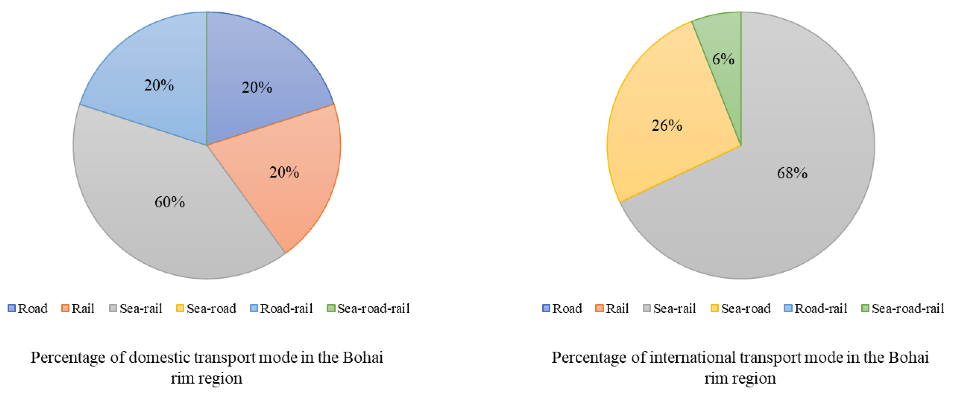
II. In order to verify the different transport modes in the intermodal and domestic transports, we have summarized the percentages of domestic and international transport modes under different objectives in the Bohai Rim region (see Figure 6).
The results show that domestic and international transport modes are different. When intermodal participants are planning their routes for goods, they need to identify whether they are domestic or international goods. If the goods are coming from foreign countries, sea-rail, sea-road, and sea-road-rail transports should be considered. It is economically advantageous to choose road, rail, road-rail, and sea-rail transport in domestic transports. Sea-rail transport accounts for the largest proportion of the domestic and international transports, which illustrates that sea-rail transport should become the most popular transport mode and developing the sea-rail transport is profitable for the intermodal participants’ operation.
III. Again, in order to prove the validity of the proposed model, changes in transport routes and modes of transport are varied by adjusting the volumes of goods. Here, we have selected Baotou as the destination. Table 8 shows the different route optimization choices and the respective freight volume conditions in these two paths.
The results show that various freight volumes lead to different transport modes and route choices. Incidentally, the results have also revealed that the model can handle high-volume shipments and that the volume factor has strong sensitivity in this model. The increase in the volume of transports corresponds with the increased likelihood of using sea-rail intermodal transport in balancing the relationships amongst costs, times, and carbon emissions. This holds true irrespective of the fact that intermodal participants may have a strong level of transport time sensitivity. Intermodal participants should consider sea-rail or rail transport for high volumes of goods as an optimal solution. Sea-road and road transport is more suitable for media and small cargo volumes.
IV. Upon close scrutiny of Figure 5 in Section 4.3, we have found that compared with single-objective optimization, the routes and modes are changeable with the difference between the origins and destinations when considering multi-objective optimization. We have also observed that the multi-objective models correlate with the three objective values in the domestic transport mode, whereas the multi-objective models enhance the three objective values when dry ports are far away from seaports in international transports. When intermodal transport participants are planning routes for their domestic goods, they will have an improved solution when they use the multi-objective models. When the intermodal transport participants are planning routes for international goods and taking account of multi-objectives in the background, they should consider the distances between the seaports and the dry ports. With the changing distances between the seaports and the dry ports, different transport mode choices should be considered.
Although the location-routing issue has been studied in detail in the distribution field [9,31], the application of the location-routing issue has gained less attention in intermodal transport. Fazayeli et al. (2018) presented intermodal transport location-routing optimizations [11]. However, this optimization methodology should be further studied in a multi-objective mode and applied to real situations. This paper proposes a two-phase approach in devotion to coping with multi-objective location-routing intermodal transport optimization problems and applies this approach to a real case, which supplements theoretical research on multi-objective location-routing intermodal transport optimization problems and provides practical insights for intermodal participants planning routes in the Bohai Rim region.
6. Conclusions
This paper analyzes the optimization of transport route choice problems using several transport modes with factors governing costs, carbon emissions, and time. Following the process of node selection, multi-objective models and GAs are used to optimize the intermodal network routes. This two-phase approach is suitable in addressing route optimization in large-scale scenarios due to the node selections and application of GA. Moreover, the model considers sustainability and time in order to ensure environmental improvement and service optimization in the field of transport. Thus, the proposed model is more comprehensive compared to the single-objective model. In particular, the proposed model is applied to the Bohai Rim region in terms of its validity. According to different market demand preferences of the intermodal participants, it provides effective intermodal transport route optimization solutions for them. Meanwhile, it can also be used in different economic regions and offers theoretical insights into other related areas. To sum up, from the practical perspectives, this paper applied the two-phase approach to the Bohai Rim region, which proves its effectiveness and provides practical insights concerning location-routing intermodal transport for intermodal participants. From the theoretical perspective, although the literature has conducted detailed research on intermodal route optimization, the intermodal location-routing issue obtained less attention. Fazayeli (2018) began to study the intermodal location-routing issues by considering the minimum total costs [11]. On this basis, this paper further studies the intermodal location-routing issue with goals of multi-objective optimization and meeting intermodal participants’ preferences. It also makes contributions to the theoretical supports for the multi-objective intermodal transport field.
The analysis brings about several insights for the intermodal participants on the optimal intermodal route under the regional intermodal transports. Under the multi-objective model, various objective weights can result in the selection of different transport modes. Therefore, it is necessary to consider the different objective preferences of the intermodal participants. By dynamically adjusting the objective preferences of intermodal participants with considerations of customer demand preferences, this approach can realize profit maximization and improve the core competition of this enterprise. Furthermore, the location of dry ports and seaports can affect the choice of transport modes and routes. With changing distances between the seaport and dry port, different transport modes should be considered. Freight volumes tend to influence the options of transport routes and means. Intermodal participants should consider sea-rail transport for high volumes of goods as an optimal solution, although the intermodal participants prefer strong time sensitivity. Meanwhile, compared to the single-objective model, the three values in the multi-objective model become more balanced, which means that the latter offers more flexible transport route optimizations than the former. In terms of research limitations and future work, this paper assumes that goods are transported to dry ports. Thus, future works in this area should include a distribution problem, which assumes that goods are transported to customers. This issue also deserves further study by taking demand uncertainty into account. Furthermore, the dry ports can be seen as a distribution hub, and further research should consider how to integrate demands from the near cities and how to decide the influence area of the dry ports in an intermodal transport system. On this basis, further considering customer demand uncertainty is a more difficult research issue. In addition, this paper presents a two-phase approach (two steps) to solve intermodal location-route problems without joint optimization. Joint location-route optimization issues will require further study in the intermodal transport field. Finally, the intermodal transport location-routing optimization should further consider transport uncertainties, such as transport time uncertainty and facility disruption uncertainty.
Author Contributions
Conceptualization, B.H.; methodology, S.S.; software, S.S.; validation, B.H., S.S., H.G. and Y.H.; formal analysis, H.G.; data curation, Y.H.; writing—original draft preparation, S.S.; writing—review and editing, S.S.; visualization, H.G.; supervision, B.H.; project administration, B.H.; funding acquisition, B.H. All authors have read and agreed to the published version of the manuscript.
Funding
This research was funded by the National Key Research and Development Project [Grant No. 2019YFB1600400], National Natural Science Foundation of China [Grant No. 72173013], the State Key Program of the National Natural Science Foundation of China [Grant No. 71831002], and the Program for Innovative Research Team in the University of the Ministry of Education of China [IRT_17R13].
Institutional Review Board Statement
Not applicable.
Informed Consent Statement
Not applicable.
Data Availability Statement
Not applicable.
Acknowledgments
This work was supported by the National Key Research and Development Project (Grant No. 2019YFB1600400), National Natural Science Foundation of China (Grant No. 72173013), the State Key Program of the National Natural Science Foundation of China (Grant No. 71831002), and the Program for Innovative Research Team in the University of the Ministry of Education of China (IRT_17R13).
Conflicts of Interest
The authors declare no conflict of interest.
Appendix A

Table A1.
Transportation unit cost, unit carbon emission footprint, and average speeds.
| Sea | Rail | Road | |
|---|---|---|---|
| Variable transportation cost ($/km) | 0.19 | 0.5 | 2 |
| Average speed (km/h) | 35 | 60 | 90 |
| Carbon footprint (kg/ton-km) | 0.084 | 0.205 | 0.472 |
Table A2.
Transfer time matrix between transportation modes (h).
| Sea | Rail | Road | |
|---|---|---|---|
| Sea | 0.7 | 0.17 | 0.17 |
| Rail | 0.17 | 0.4 | 0.12 |
| Road | 0.17 | 0.12 | 0.1 |
Table A3.
Transfer cost matrix (USD/15 tones container).
| Sea | Rail | Road | |
| Sea | 100 | 150 | 88 |
| Rail | 150 | 80 | 100 |
| Road | 88 | 100 | 50 |
Table A4.
Rail transport distance in domestic transportation networks.
| Guangzhou | Dalian | Tianjin | Qingdao | Shenyang | Beijing | Tangshan | Shijiazhuang | Jinan | Changchun | Huhhot | Baotou | Taiyuan | Harbin | |
|---|---|---|---|---|---|---|---|---|---|---|---|---|---|---|
| Zhanjiang | 432 | - | - | - | - | - | - | - | - | - | - | - | - | - |
| Guangzhou | - | 3264 | 2374 | 2121 | 3078 | 2478 | 2455 | 2199 | 2027 | 3393 | 2840 | 3112 | 2251 | 3753 |
| Dalian | - | - | 1104 | - | 397 | 1138 | 722 | 1523 | 1464 | 702 | 1805 | 1957 | 1652 | 944 |
| Tianjin | - | - | - | 753 | 707 | 137 | 123 | 419 | 360 | 1012 | 804 | 961 | 650 | 1254 |
| Qingdao | - | - | - | - | 1460 | 953 | 818 | 822 | 393 | 1765 | 1557 | 1777 | 925 | 2007 |
| Shenyang | - | - | - | - | - | 741 | 552 | 1126 | 1067 | 305 | 1408 | 1560 | 1255 | 547 |
| Beijing | - | - | - | - | - | - | 151 | 283 | 497 | 1046 | 667 | 824 | 514 | 1288 |
| Tangshan | - | - | - | - | - | - | - | 420 | 579 | 866 | 802 | 975 | 643 | 1105 |
| Shijiazhuang | - | - | - | - | - | - | - | - | 301 | 1431 | 871 | 1069 | 231 | 1673 |
| Jinan | - | - | - | - | - | - | - | - | - | 1372 | 1164 | 1213 | 532 | 1614 |
| Changchun | - | - | - | - | - | - | - | - | - | - | 1713 | 1639 | 1560 | 242 |
| Huhhot | - | - | - | - | - | - | - | - | - | - | - | 272 | 640 | 1955 |
| Baotou | - | - | - | - | - | - | - | - | - | - | - | - | 668 | 1878 |
| Taiyuan | - | - | - | - | - | - | - | - | - | - | - | - | - | 1802 |
Table A5.
Road transport distance in domestic transportation networks.
| Guangzhou | Dalian | Tianjin | Qingdao | Shenyang | Beijing | Tangshan | Shijiazhuang | Jinan | Changchun | Huhhot | Baotou | Taiyuan | Harbin | |
|---|---|---|---|---|---|---|---|---|---|---|---|---|---|---|
| Zhanjiang | 416.5 | 3243.6 | 2441.2 | 2310.7 | 3100.4 | 2458 | 2551.9 | 2191.5 | 2168.9 | 3376.7 | 2639.2 | 2786.2 | 2207.7 | 3708.7 |
| Guangzhou | - | 2899.1 | 2096.2 | 1907.5 | 2756 | 2112.7 | 2206.9 | 1846.2 | 1823.2 | 3032.5 | 2294.1 | 2441.2 | 1862.6 | 3363.9 |
| Dalian | - | - | 824 | 397 | 379 | 840 | 702 | 1105 | 1122 | 676 | 1313 | 1488 | 1304 | 936 |
| Tianjin | - | - | - | 527 | 679 | 134 | 131 | 314 | 330 | 956 | 612 | 787 | 513 | 1293 |
| Qingdao | - | - | - | - | 1176 | 652 | 637 | 644 | 351 | 1452 | 1131 | 1306 | 852 | 1790 |
| Shenyang | - | - | - | - | - | 696 | 558 | 962 | 979 | 308 | 1170 | 1345 | 1163 | 567 |
| Beijing | - | - | - | - | - | - | 179 | 292 | 410 | 972 | 482 | 657 | 490 | 1287 |
| Tangshan | - | - | - | - | - | - | - | 424 | 440 | 834 | 654 | 828 | 622 | 1172 |
| Shijiazhuang | - | - | - | - | - | - | - | - | 327 | 1237 | 593 | 765 | 224 | 1574 |
| Jinan | - | - | - | - | - | - | - | - | - | 1256 | 864 | 1037 | 522 | 1593 |
| Changchun | - | - | - | - | - | - | - | - | - | - | 1413 | 1587 | 1446 | 254 |
| Huhhot | - | - | - | - | - | - | - | - | - | - | - | 180 | 440 | 1721 |
| Baotou | - | - | - | - | - | - | - | - | - | - | - | 618 | 1902 | |
| Taiyuan | - | - | - | - | - | - | - | - | - | - | - | - | 1773 |
Table A6.
Sea transport distance in domestic transportation networks.
| Guangzhou | Dalian | Tianjin | Qingdao | Shenyang | Beijing | Tangshan | Shijiazhuang | Jinan | Changchun | Huhhot | Baotou | Taiyuan | Harbin | |
|---|---|---|---|---|---|---|---|---|---|---|---|---|---|---|
| Zhanjiang | - | 2683.8 | 2939.4 | 2426.4 | - | - | - | - | - | - | - | - | - | - |
| Guangzhou | - | - | - | - | - | - | - | - | - | - | - | - | - | - |
| Dalian | - | - | - | - | - | - | - | - | - | - | - | - | - | - |
| Tianjin | - | - | - | - | - | - | - | - | - | - | - | - | - | - |
| Qingdao | - | - | - | - | - | - | - | - | - | - | - | - | - | - |
| Shenyang | - | - | - | - | - | - | - | - | - | - | - | - | - | - |
| Beijing | - | - | - | - | - | - | - | - | - | - | - | - | - | - |
| Tangshan | - | - | - | - | - | - | - | - | - | - | - | - | - | - |
| Shijiazhuang | - | - | - | - | - | - | - | - | - | - | - | - | - | - |
| Jinan | - | - | - | - | - | - | - | - | - | - | - | - | - | - |
| Changchun | - | - | - | - | - | - | - | - | - | - | - | - | - | - |
| Huhhot | - | - | - | - | - | - | - | - | - | - | - | - | - | - |
| Baotou | - | - | - | - | - | - | - | - | - | - | - | - | - | - |
| Taiyuan | - | - | - | - | - | - | - | - | - | - | - | - | - | - |
Table A7.
Rail transport distance in international transportation networks.
| Dalian | Tianjin | Qingdao | Shenyang | Beijing | Tangshan | Shijiazhuang | Jinan | Changchun | Huhhot | Baotou | Taiyuan | Harbin | |
|---|---|---|---|---|---|---|---|---|---|---|---|---|---|
| Busan | - | - | - | - | - | - | - | - | - | - | - | - | - |
| Dalian | - | 1104 | - | 397 | 1138 | 722 | 1523 | 1464 | 702 | 1805 | 1957 | 1652 | 944 |
| Tianjin | - | - | 753 | 707 | 137 | 123 | 419 | 360 | 1012 | 804 | 961 | 650 | 1254 |
| Qingdao | - | - | - | 1460 | 953 | 818 | 822 | 393 | 1765 | 1557 | 1777 | 925 | 2007 |
| Shenyang | - | - | - | - | 741 | 552 | 1126 | 1067 | 305 | 1408 | 1560 | 1255 | 547 |
| Beijing | - | - | - | - | - | 151 | 283 | 497 | 1046 | 667 | 824 | 514 | 1288 |
| Tangshan | - | - | - | - | - | - | 420 | 579 | 866 | 802 | 975 | 643 | 1105 |
| Shijiazhuang | - | - | - | - | - | - | - | 301 | 1431 | 871 | 1069 | 231 | 1673 |
| Jinan | - | - | - | - | - | - | - | - | 1372 | 1164 | 1213 | 532 | 1614 |
| Changchun | - | - | - | - | - | - | - | - | - | 1713 | 1639 | 1560 | 242 |
| Huhhot | - | - | - | - | - | - | - | - | - | - | 165 | 640 | 1955 |
| Baotou | - | - | - | - | - | - | - | - | - | - | - | 668 | 1878 |
| Taiyuan | - | - | - | - | - | - | - | - | - | - | - | - | 1802 |
Table A8.
Road transport distance in international transportation networks.
| Dalian | Tianjin | Qingdao | Shenyang | Beijing | Tangshan | Shijiazhuang | Jinan | Changchun | Huhhot | Baotou | Taiyuan | Harbin | |
|---|---|---|---|---|---|---|---|---|---|---|---|---|---|
| Busan | - | - | - | - | - | - | - | - | - | - | - | - | - |
| Dalian | - | 824 | 397 | 379 | 840 | 702 | 1105 | 1122 | 676 | 1313 | 1488 | 1304 | 936 |
| Tianjin | - | - | 527 | 679 | 134 | 131 | 314 | 330 | 956 | 612 | 787 | 513 | 1293 |
| Qingdao | - | - | - | 1176 | 652 | 637 | 644 | 351 | 1452 | 1131 | 1306 | 852 | 1790 |
| Shenyang | - | - | - | - | 696 | 558 | 962 | 979 | 308 | 1170 | 1345 | 1163 | 567 |
| Beijing | - | - | - | - | - | 179 | 292 | 410 | 972 | 482 | 657 | 490 | 1287 |
| Tangshan | - | - | - | - | - | - | 424 | 440 | 834 | 654 | 828 | 622 | 1172 |
| Shijiazhuang | - | - | - | - | - | - | - | 327 | 1237 | 593 | 765 | 224 | 1574 |
| Jinan | - | - | - | - | - | - | - | - | 1256 | 864 | 1037 | 522 | 1593 |
| Changchun | - | - | - | - | - | - | - | - | - | 1413 | 1587 | 1446 | 254 |
| Huhhot | - | - | - | - | - | - | - | - | - | - | 180 | 440 | 1721 |
| Baotou | - | - | - | - | - | - | - | - | - | - | - | 618 | 1902 |
| Taiyuan | - | - | - | - | - | - | - | - | - | - | - | - | 1773 |
Table A9.
Sea transport distance in international transportation networks.
| Dalian | Tianjin | Qingdao | Shenyang | Beijing | Tangshan | Shijiazhuang | Jinan | Changchun | Huhhot | Baotou | Taiyuan | Harbin | |
|---|---|---|---|---|---|---|---|---|---|---|---|---|---|
| Busan | 982.8 | 1324.8 | 891 | - | - | - | - | - | - | - | - | - | - |
| Dalian | - | - | - | - | - | - | - | - | - | - | - | - | - |
| Tianjin | - | - | - | - | - | - | - | - | - | - | - | - | - |
| Qingdao | - | - | - | - | - | - | - | - | - | - | - | - | - |
| Shenyang | - | - | - | - | - | - | - | - | - | - | - | - | - |
| Beijing | - | - | - | - | - | - | - | - | - | - | - | - | - |
| Tangshan | - | - | - | - | - | - | - | - | - | - | - | - | - |
| Shijiazhuang | - | - | - | - | - | - | - | - | - | - | - | - | - |
| Jinan | - | - | - | - | - | - | - | - | - | - | - | - | - |
| Changchun | - | - | - | - | - | - | - | - | - | - | - | - | - |
| Huhhot | - | - | - | - | - | - | - | - | - | - | - | - | - |
| Baotou | - | - | - | - | - | - | - | - | - | - | - | - | - |
| Taiyuan | - | - | - | - | - | - | - | - | - | - | - | - | - |
Table A10.
Different route optimization choices considering single-objective optimizations in domestic networks.
Table A10.
Different route optimization choices considering single-objective optimizations in domestic networks.
| Task | Origin | Destination | Intermodal Transport Route | Cost | Time | Carbon Emission |
|---|---|---|---|---|---|---|
| Lowest Cost | ||||||
| 1 | Zhanjiang | Harbin | 19,838.44 | 103.17 | 8379.184 | |
| 2 | Zhanjiang | Taiyuan | 17,869.720 | 106.17 | 7603.192 | |
| 3 | Zhanjiang | Baotou | 20,979.720 | 111.170 | 8878.292 | |
| 4 | Zhanjiang | Huhhot | 19,409.720 | 109.170 | 8234.592 | |
| 5 | Zhanjiang | Changchun | 17,418. 440 | 99.170 | 7386.984 | |
| 6 | Zhanjiang | Jinan | 13,350.320 | 88.170 | 5687.652 | |
| 7 | Zhanjiang | Shijiazhuang | 15,559.720 | 102.170 | 6656.092 | |
| 8 | Zhanjiang | Tangshan | 12,599.720 | 97.170 | 5442.492 | |
| 9 | Zhanjiang | Beijing | 12,739.720 | 98.170 | 5499.892 | |
| 10 | Zhanjiang | Shenyang | 14,368.440 | 94.170 | 6136.484 | |
| Fastest Time | ||||||
| 1 | Zhanjiang | Harbin | 148,348.000 | 50.008 | 35,010.128 | |
| 2 | Zhanjiang | Taiyuan | 88,308.000 | 33.33 | 20,840.688 | |
| 3 | Zhanjiang | Baotou | 111,448.000 | 39.758 | 26,301.728 | |
| 4 | Zhanjiang | Huhhot | 105,568.000 | 38.124 | 24,914.048 | |
| 5 | Zhanjiang | Changchun | 135,068.000 | 46.319 | 31,876.048 | |
| 6 | Zhanjiang | Jinan | 86,756.000 | 32.899 | 20,474.416 | |
| 7 | Zhanjiang | Shijiazhuang | 87,660.000 | 33.150 | 20,687.760 | |
| 8 | Zhanjiang | Tangshan | 102,076.000 | 37.154 | 24,089.936 | |
| 9 | Zhanjiang | Beijing | 98,320.000 | 36.111 | 23,203.520 | |
| 10 | Zhanjiang | Shenyang | 124,016.000 | 43.249 | 29,267.776 | |
| Lowest Carbon Emission | ||||||
| 1 | Zhanjiang | Harbin | 19,838.440 | 103.17 | 8379.184 | |
| 2 | Zhanjiang | Taiyuan | 17,869.720 | 106.17 | 7603.192 | |
| 3 | Zhanjiang | Baotou | 20,979.720 | 111.170 | 8878.292 | |
| 4 | Zhanjiang | Huhhot | 19,409.720 | 109.170 | 8234.592 | |
| 5 | Zhanjiang | Changchun | 17,418.440 | 99.170 | 7386.984 | |
| 6 | Zhanjiang | Jinan | 13,350.320 | 88.170 | 5687.652 | |
| 7 | Zhanjiang | Shijiazhuang | 15,559.720 | 102.170 | 6656.092 | |
| 8 | Zhanjiang | Tangshan | 12,599.720 | 97.170 | 5442.492 | |
| 9 | Zhanjiang | Beijing | 12,739.720 | 98.170 | 5499.892 | |
| 10 | Zhanjiang | Shenyang | 14,368.440 | 94.170 | 6136.484 | |
Table A11.
Different route optimization choices considering single-objective optimizations in international networks.
Table A11.
Different route optimization choices considering single-objective optimizations in international networks.
| Task | Origin | Destination | Intermodal Transport Route | Cost | Time | Carbon Emission |
|---|---|---|---|---|---|---|
| Lowest Cost | ||||||
| 1 | Busan | Harbin | 13,374.640 | 55.170 | 5521.504 | |
| 2 | Busan | Taiyuan | 11,734.240 | 60.170 | 4890.664 | |
| 3 | Busan | Baotou | 14,844.240 | 65.170 | 6165.764 | |
| 4 | Busan | Huhhot | 13,274.240 | 63.170 | 5522.064 | |
| 5 | Busan | Changchun | 10,954.640 | 51.170 | 4529.304 | |
| 6 | Busan | Jinan | 7515.800 | 44.170 | 3108.180 | |
| 7 | Busan | Shijiazhuang | 9424.240 | 56.170 | 3943.564 | |
| 8 | Busan | Tangshan | 6464.240 | 51.170 | 2729.964 | |
| 9 | Busan | Beijing | 6604.240 | 52.170 | 2787.364 | |
| 10 | Busan | Shenyang | 7904.640 | 46.170 | 3278.804 | |
| Fastest Time | ||||||
| 1 | Busan | Harbin | 41,292.040 | 49.370 | 10,486.944 | |
| 2 | Busan | Taiyuan | 37,583.200 | 46.437 | 9539.760 | |
| 3 | Busan | Baotou | 55,743.200 | 51.481 | 13,825.520 | |
| 4 | Busan | Huhhot | 48,743.200 | 49.537 | 12,173.520 | |
| 5 | Busan | Changchun | 30,892.040 | 46.481 | 8032.544 | |
| 6 | Busan | Jinan | 17,543.2 | 40.87 | 4810.32 | |
| 7 | Busan | Shijiazhuang | 28,983.200 | 44.048 | 7510.160 | |
| 8 | Busan | Tangshan | 29,263.200 | 44.126 | 7576.240 | |
| 9 | Busan | Beijing | 17,543.200 | 40.870 | 4810.320 | |
| 10 | Busan | Shenyang | 19,012.040 | 43.181 | 5228.864 | |
| Lowest Carbon Emission | ||||||
| 1 | Busan | Harbin | 13,374.640 | 55.170 | 5521.504 | |
| 2 | Busan | Taiyuan | 11,734.240 | 60.170 | 4890.664 | |
| 3 | Busan | Baotou | 14,844.240 | 65.170 | 6165.764 | |
| 4 | Busan | Huhhot | 13,274.240 | 63.170 | 5522.064 | |
| 5 | Busan | Changchun | 10,954.640 | 51.170 | 4529.304 | |
| 6 | Busan | Jinan | 7515.800 | 44.170 | 3108.180 | |
| 7 | Busan | Shijiazhuang | 9424.240 | 56.170 | 3943.564 | |
| 8 | Busan | Tangshan | 6464.240 | 51.170 | 2729.964 | |
| 9 | Busan | Beijing | 6604.240 | 52.170 | 2787.364 | |
| 10 | Busan | Shenyang | 7904.640 | 46.170 | 3278.804 | |
References
- Duan, X.; Heragu, S. Carbon Emission Tax Policy in an Intermodal Transport Network. In IIE Annual Conference. Proceedings; Institute of Industrial and Systems Engineers (IISE): Norcross, GA, USA, 2015; p. 566. [Google Scholar]
- He, J.; Huang, Y.; Chang, D. Simulation-based heuristic method for container supply chain network optimization. Adv. Eng. Inform. 2015, 29, 339–354. [Google Scholar] [CrossRef]
- Göçmen, E.; Erol, R. The problem of sustainable intermodal transport: A case study of an international logistics company, turkey. Sustainability 2018, 10, 4268. [Google Scholar] [CrossRef] [Green Version]
- Roso, V.; Woxenius, J.; Lumsden, K. The dry port concept: Connecting container seaports with the hinterland. J. Transp. Geogr. 2009, 17, 338–345. [Google Scholar] [CrossRef]
- Idri, A.; Oukarfi, M.; Boulmakoul, A.; Zeitouni, K.; Masri, A. A new time-dependent shortest path algorithm for multimodal transport network. Procedia Comput. Sci. 2017, 109, 692–697. [Google Scholar] [CrossRef]
- Munim, Z.H.; Haralambides, H. Competition and cooperation for intermodal container transhipment: A network optimization approach. Res. Transp. Bus. Manag. 2018, 26, 87–99. [Google Scholar] [CrossRef]
- Wang, X.; Meng, Q. Discrete intermodal freight transport network design with route choice behavior of intermodal operators. Transp. Res. Part B Methodol. 2017, 95, 76–104. [Google Scholar] [CrossRef]
- Wang, Y.; Peng, S.; Zhou, X.; Mahmoudi, M.; Zhen, L. Green logistics location-routing problem with eco-packages. Transp. Res. Part E Logist. Transp. Rev. 2020, 143, 102118. [Google Scholar] [CrossRef]
- Nataraj, S.; Ferone, D.; Quintero-Araujo, C.; Juan, A.; Festa, P. Consolidation centers in city logistics: A cooperative approach based on the location routing problem. Int. J. Ind. Eng. Comput. 2019, 10, 393–404. [Google Scholar] [CrossRef]
- Chen, J.; Gui, P.; Ding, T.; Na, S.; Zhou, Y. Optimization of transportation routing problem for fresh food by improved ant colony algorithm based on tabu search. Sustainability 2019, 11, 6584. [Google Scholar] [CrossRef] [Green Version]
- Fazayeli, S.; Eydi, A.; Kamalabadi, I.N. Location-routing problem in multimodal transport network with time windows and fuzzy demands: Presenting a two-part genetic algorithm. Comput. Ind. Eng. 2018, 119, 233–246. [Google Scholar] [CrossRef]
- Nasrollahi, M.; Fathi, M.R.; Hassani, N.S. Eco-innovation and cleaner production as sustainable competitive advantage antecedents: The mediating role of green performance. Int. J. Bus. Innov. Res. 2020, 22, 388–407. [Google Scholar] [CrossRef]
- Nasrollahi, M.; Fathi, M.R.; Sanouni, H.R.; Sobhani, S.M.; Behrooz, A. Impact of coercive and non-coercive environmental supply chain sustainability drivers on supply chain performance: Mediation role of monitoring and collaboration. Int. J. Sustain. Eng. 2021, 14, 98–106. [Google Scholar] [CrossRef]
- Lam, J.S.L.; Gu, Y. A market-oriented approach for intermodal network optimisation meeting cost 1987, time and environmental requirements. Int. J. Prod. Econ. 2016, 171, 266–274. [Google Scholar] [CrossRef]
- Resat, H.G.; Turkay, M. A bi-objective model for design and analysis of sustainable intermodal transport systems: A case study of Turkey. Int. J. Prod. Res. 2019, 57, 6146–6161. [Google Scholar] [CrossRef]
- Mostert, M.; Caris, A.; Limbourg, S. Intermodal network design: A three-mode bi-objective model applied to the case of Belgium. Flex. Serv. Manuf. J. 2018, 30, 397–420. [Google Scholar] [CrossRef] [Green Version]
- Gohari, A.; Nasir Matori, A.; Yusof, K.W.; Toloue, I.; Myint, K.C.; Sholagberu, A.T. Route/Modal choice analysis and tradeoffs evaluation of the intermodal transport network of Peninsular Malaysia. Cogent Eng. 2018, 5, 1436948. [Google Scholar] [CrossRef]
- Göçmen, E.; Erol, R. Transport problems for intermodal networks: Mathematical models, exact and heuristic algorithms, and machine learning. Expert Syst. Appl. 2019, 135, 374–387. [Google Scholar] [CrossRef]
- Dai, Q.; Yang, J.; Li, D. Modeling a three-mode two-phase port-hinterland freight intermodal distribution network with environmental consideration: The case of the Yangtze river economic belt in China. Sustainability 2018, 10, 3081. [Google Scholar] [CrossRef] [Green Version]
- Zhao, Y.; Yang, Z.; Haralambides, H. Optimizing the transport of export containers along China’s coronary artery: The Yangtze River. J. Transp. Geogr. 2019, 77, 11–25. [Google Scholar] [CrossRef]
- Lu, W.; Park, S.H.; Liu, S.; Nam, T.H.; Yeo, G.T. Connection analysis of container ports of the Bohai Rim Economic Circle (BREC). Asian J. Shipp. Logist. 2018, 34, 145–150. [Google Scholar] [CrossRef]
- Meraklı, M.; Yaman, H. Robust intermodal hub location under polyhedral demand uncertainty. Transp. Res. Part B Methodol. 2016, 86, 66–85. [Google Scholar] [CrossRef] [Green Version]
- Caris, A.; Macharis, C.; Janssens, G.K. Decision support in intermodal transport: A new research agenda. Comput. Ind. 2013, 64, 105–112. [Google Scholar] [CrossRef]
- Chang, Z.; Notteboom, T.; Lu, J. A two-phase model for dry port location with an application to the port of Dalian in China. Transp. Plan. Technol. 2015, 38, 442–464. [Google Scholar] [CrossRef]
- Van Nguyen, T.; Zhang, J.; Zhou, L.; Meng, M.; He, Y. A data-driven optimization of large-scale dry port location using the two-phase approach of data mining and complex network theory. Transp. Res. Part E Logist. Transp. Rev. 2020, 134, 101816. [Google Scholar] [CrossRef]
- Wang, R.; Yang, K.; Yang, L.; Gao, Z. Modeling and optimization of a road–rail intermodal transport system under uncertain information. Eng. Appl. Artif. Intell. 2018, 72, 423–436. [Google Scholar] [CrossRef]
- Kaddani, S.; Vanderpooten, D.; Vanpeperstraete, J.M.; Aissi, H. Weighted sum model with partial preference information: Application to multi-objective optimization. Eur. J. Oper. Res. 2017, 260, 665–679. [Google Scholar] [CrossRef]
- Majidi, M.; Nojavan, S.; Esfetanaj, N.N.; Najafi-Ghalelou, A.; Zare, K. A multi-objective model for optimal operation of a battery/PV/fuel cell/grid two-phase energy system using weighted sum technique and fuzzy satisfying approach considering responsible load management. Sol. Energy 2017, 144, 79–89. [Google Scholar] [CrossRef]
- Lin, C.; Gao, F.; Bai, Y. An intelligent sampling approach for metamodel-based multi-objective optimization with guidance of the adaptive weighted-sum method. Struct. Multidiscip. Optim. 2018, 57, 1047–1060. [Google Scholar] [CrossRef]
- Hrušovský, M.; Demir, E.; Jammernegg, W.; Van Woensel, T. Real-time disruption management approach for intermodal freight transport. J. Clean. Prod. 2021, 280, 124826. [Google Scholar] [CrossRef]
- Wang, C.N.; Nhieu, N.L.; Chung, Y.C.; Pham, H.T. Multi-objective optimization models for sustainable perishable intermodal multi-product networks with delivery time window. Mathematics 2021, 9, 379. [Google Scholar] [CrossRef]
Figure 1.
Flowchart of the two-phase approach.

Figure 2.
The process of MILP model.

Figure 3.
Intermodal network in the Bohai Rim region.

Figure 4.
Pareto solutions of intermodal transportation problem.

Figure 5.
Comparison of the costs, times, and carbon emissions of each objective in intermodal transport.
Figure 5.
Comparison of the costs, times, and carbon emissions of each objective in intermodal transport.

Figure 6.
The percentage of domestic and international transport mode in different objectives.

Table 1.
Literature review of the related works.
| Authors and Year | Intermodal Route Problem | Intermodal Location-Route Problem | Multi-Objective | Sustainability Problem | Model | Solving Approach | Real Application |
|---|---|---|---|---|---|---|---|
| Idri et al. (2017) | √ | - | - | - | the shortest paths | - | - |
| Munima (2018) | √ | - | - | - | MIP model | - | - |
| Wang and Meng (2017) | √ | - | - | - | Mixed-integer nonlinear | Non-convex program | - |
| Saeed Fazayeli (2018) | √ | √ | - | - | MIP fuzzy model | A two-part GA | - |
| Resat and Turkay (2019) | √ | - | √ | √ | Mixed-integer linear optimization model | Exact solution methods | √ |
| Mostert et al. (2018) | √ | - | √ | √ | Bi-objective mathematical formulation | CPLEX | √ |
| Gohari et al. (2018) | √ | - | - | - | - | ArcMap software; the shortest path algorithm | √ |
| Göçmen and Erol (2019) | √ | √ | - | - | Mathematical models | Exact and heuristic algorithms | √ |
| Dai et al. (2018) | √ | - | √ | √ | - | Distribution network topology | √ |
| Zhao et al. (2019) | √ | - | - | - | - | Super networks | √ |
| Seo et al. (2017) | √ | - | - | - | Multimodal Transport Cost-Model | - | √ |
| Mohammad and Hector (2016) | √ | √ | - | - | Path-based formulation | Decomposition-based search algorithm | √ |
| The current work | √ | √ | √ | √ | MILP | FCM; GA | √ |
Table 2.
Evaluation system for node location decisions.
| Influencing Factors | Quantitative Indexes |
|---|---|
| Regional economy | X1 Gross regional product |
| Foreign trade | X2 Total value of imports and exports |
| Transportation system | X3 Urban road area |
| X4 Transport freight volume | |
| X5 Urban connectivity | |
| Consumption level | X6 Total retail sales of social consumer goods |
Table 3.
Sets, decision variables, and parameters used in the linear programming model.
| Sets | |
| Set of all nodes | |
| Nodes passed on the way to completion of transport tasks | |
| Set of all transportation modes | |
| Set of all transportation modes | |
| M | Set of all transportation tasks |
| Decision Variables | |
| If task is transported by between nodes and , then , otherwise it is 0 | |
| If task is converted from transport mode to transport mode at node , then , otherwise it is 0 | |
| Parameters | |
| Unit variable cost for mode of transport between nodes and | |
| Unit changeover cost for node converted from transport mode to transport mode s | |
| Conversion time for node to change from transport mode to transport mode s | |
| Transport distance between nodes and using transport mode | |
| Transport speed of transport mode between nodes and | |
| Maximum transport capacity of transport mode between nodes and | |
| Volume of transport task | |
| Carbon emissions per unit of transport mode | |
Table 4.
Level of sensitivity transport cost, time and carbon emission.
| Numerical Representation | Level of Sensitivity | ||
|---|---|---|---|
| Strong | General | Weak | |
| Numerical value | 7 | 5 | 3 |
Table 5.
Fuzzy clustering centers.
| Category | X1 | X2 | X3 | X4 | X5 | X6 |
|---|---|---|---|---|---|---|
| I | 277.49 | 318.16 | 10.47 | 19.79 | 2.11 | 114.13 |
| II | 63.99 | 26.66 | 8.35 | 24.31 | 3.64 | 39.07 |
| III | 28.37 | 12.12 | 7.05 | 26.36 | 2.53 | 23.18 |
| Ⅳ | 5.66 | 1.71 | 1.65 | 8.62 | 2.37 | 6.27 |
Table 6.
Membership degrees of cities.
| City | I | II | III | Ⅳ | City | I | II | III | Ⅳ | City | I | II | III | Ⅳ |
|---|---|---|---|---|---|---|---|---|---|---|---|---|---|---|
| Changchun | 0.00 | 0.52 | 0.38 | 0.10 | Harbin | 0.00 | 0.41 | 0.48 | 0.11 | Qitaihe | 0.00 | 0.01 | 0.05 | 0.94 |
| Jilin | 0.00 | 0.03 | 0.14 | 0.83 | Qiqihar | 0.00 | 0.00 | 0.02 | 0.97 | Mudanjiang | 0.00 | 0.01 | 0.02 | 0.97 |
| Siping | 0.00 | 0.02 | 0.11 | 0.87 | Jixi | 0.00 | 0.01 | 0.03 | 0.96 | Heihe | 0.00 | 0.02 | 0.05 | 0.93 |
| Liaoyuan | 0.00 | 0.01 | 0.04 | 0.96 | Hegang | 0.00 | 0.01 | 0.05 | 0.94 | Suihua | 0.00 | 0.01 | 0.03 | 0.96 |
| Tonghua | 0.00 | 0.01 | 0.03 | 0.96 | Shuangyashan | 0.00 | 0.01 | 0.05 | 0.94 | Shenyang | 0.00 | 0.65 | 0.28 | 0.06 |
| Baishan | 0.00 | 0.01 | 0.04 | 0.95 | Daqing | 0.00 | 0.07 | 0.34 | 0.59 | Dalian | 0.00 | 0.57 | 0.35 | 0.08 |
| Songyuan | 0.00 | 0.00 | 0.01 | 0.99 | Yichun | 0.00 | 0.02 | 0.05 | 0.93 | Anshan | 0.00 | 0.03 | 0.17 | 0.80 |
| Baicheng | 0.00 | 0.01 | 0.04 | 0.95 | Jiamusi | 0.00 | 0.01 | 0.97 | 0.97 | Fushun | 0.00 | 0.00 | 0.01 | 0.99 |
| Benxi | 0.00 | 0.00 | 0.01 | 0.99 | Chaoyang | 0.00 | 0.01 | 0.02 | 0.98 | Hulunbuir | 0.00 | 0.00 | 0.02 | 0.98 |
| Dandong | 0.00 | 0.00 | 0.01 | 0.99 | Huludao | 0.00 | 0.00 | 0.01 | 0.98 | Bayannur | 0.00 | 0.00 | 0.02 | 0.98 |
| Jinzhou | 0.00 | 0.01 | 0.06 | 0.93 | Huhhot | 0.00 | 0.18 | 0.48 | 0.34 | Ulanqab | 0.00 | 0.00 | 0.02 | 0.98 |
| Yingkou | 0.00 | 0.01 | 0.08 | 0.91 | Baotou | 0.00 | 0.12 | 0.64 | 0.23 | Taiyuan | 0.00 | 0.08 | 0.79 | 0.14 |
| Fuxin | 0.00 | 0.01 | 0.02 | 0.97 | Wuhai | 0.00 | 0.01 | 0.03 | 0.97 | Datong | 0.00 | 0.00 | 0.01 | 0.98 |
| Liaoyang | 0.00 | 0.01 | 0.03 | 0.96 | Chifeng | 0.00 | 0.02 | 0.09 | 0.90 | Yangquan | 0.00 | 0.01 | 0.02 | 0.97 |
| Panjin | 0.00 | 0.01 | 0.04 | 0.95 | Tongliao | 0.00 | 0.00 | 0.01 | 0.98 | Changzhi | 0.00 | 0.00 | 0.00 | 0.99 |
| Tieling | 0.00 | 0.00 | 0.02 | 0.98 | Ordos | 0.00 | 0.02 | 0.14 | 0.84 | Jincheng | 0.00 | 0.00 | 0.01 | 0.98 |
| Shuozhou | 0.00 | 0.01 | 0.02 | 0.97 | Qinhuangdao | 0.00 | 0.01 | 0.05 | 0.94 | Hengshui | 0.00 | 0.00 | 0.01 | 0.99 |
| Jinzhong | 0.00 | 0.00 | 0.02 | 0.98 | Handan | 0.00 | 0.05 | 0.43 | 0.52 | Jinan | 0.00 | 0.83 | 0.13 | 0.04 |
| Yuncheng | 0.00 | 0.01 | 0.05 | 0.94 | Xingtai | 0.00 | 0.03 | 0.18 | 0.79 | Qingdao | 0.02 | 0.63 | 0.23 | 0.13 |
| Xinzhou | 0.00 | 0.00 | 0.02 | 0.98 | Baoding | 0.00 | 0.04 | 0.30 | 0.66 | Zibo | 0.00 | 0.09 | 0.84 | 0.08 |
| Linfen | 0.00 | 0.01 | 0.04 | 0.96 | Zhangjiakou | 0.00 | 0.01 | 0.03 | 0.97 | Zaozhuang | 0.00 | 0.01 | 0.05 | 0.94 |
| Luliang | 0.00 | 0.00 | 0.02 | 0.98 | Chengde | 0.00 | 0.00 | 0.01 | 0.98 | Dongying | 0.00 | 0.12 | 0.46 | 0.42 |
| Shijiazhuang | 0.00 | 0.19 | 0.70 | 0.11 | Cangzhou | 0.00 | 0.04 | 0.32 | 0.63 | Yantai | 0.00 | 0.40 | 0.44 | 0.16 |
| Tangshan | 0.00 | 0.12 | 0.79 | 0.09 | Langfang | 0.00 | 0.01 | 0.04 | 0.95 | Weifang | 0.00 | 0.08 | 0.78 | 0.14 |
| Jining | 0.00 | 0.04 | 0.81 | 0.15 | Laiwu | 0.00 | 0.00 | 0.01 | 0.98 | Binzhou | 0.00 | 0.02 | 0.12 | 0.86 |
| Taian | 0.00 | 0.03 | 0.13 | 0.84 | Linyi | 0.00 | 0.06 | 0.81 | 0.13 | Heze | 0.00 | 0.03 | 0.21 | 0.75 |
| Weihai | 0.00 | 0.05 | 0.27 | 0.68 | Dezhou | 0.00 | 0.03 | 0.18 | 0.80 | Beijing | 1.00 | 0.00 | 0.00 | 0.00 |
| Rizhao | 0.00 | 0.02 | 0.07 | 0.91 | Liaocheng | 0.00 | 0.03 | 0.21 | 0.75 | Tianjin | 0.17 | 0.40 | 0.25 | 0.19 |
Table 7.
Different route optimization choices in multi-objective optimizations.
| Task | Origin | Destination | Intermodal Transport Route | Cost | Time | Carbon Emission |
|---|---|---|---|---|---|---|
| (Strong cost sensitivity) | ||||||
| 1 | Zhanjiang | Harbin | 41,956.600 | 80.400 | 17,158.500 | |
| 2 | Zhanjiang | Taiyuan | 26,936.600 | 55.400 | 11,000.300 | |
| 3 | Zhanjiang | Baotou | 35,546.600 | 69.400 | 14,530.400 | |
| 4 | Zhanjiang | Huhhot | 32,826.600 | 65.400 | 13,415.200 | |
| 5 | Zhanjiang | Changchun | 38,356.600 | 74.400 | 38,356.600 | |
| 6 | Zhanjiang | Jinan | 24,696.600 | 51.400 | 10,081.900 | |
| 7 | Zhanjiang | Shijiazhuang | 26,416.600 | 54.400 | 10,787.100 | |
| 8 | Zhanjiang | Tangshan | 28,976.600 | 58.400 | 11,836.700 | |
| 9 | Zhanjiang | Beijing | 29,206.600 | 59.400 | 11,931.000 | |
| 10 | Zhanjiang | Shenyang | 35,206.600 | 69.400 | 14,391.000 | |
| 11 | Busan | Harbin | 13,374.640 | 55.170 | 5521.504 | |
| 12 | Busan | Taiyuan | 12,835.800 | 53.170 | 5289.380 | |
| 13 | Busan | Baotou | 14,844.240 | 65.170 | 6165.764 | |
| 14 | Busan | Huhhot | 13,274.240 | 63.170 | 5522.064 | |
| 15 | Busan | Changchun | 10,954.640 | 51.170 | 4529.304 | |
| 16 | Busan | Jinan | 7515.800 | 44.170 | 3108.180 | |
| 17 | Busan | Shijiazhuang | 10,525.800 | 49.170 | 4342.280 | |
| 18 | Busan | Tangshan | 6464.240 | 51.170 | 2729.964 | |
| 19 | Busan | Beijing | 6604.240 | 52.170 | 2787.364 | |
| 20 | Busan | Shenyang | 7904.640 | 46.170 | 3278.804 | |
| (Strong time sensitivity) | ||||||
| 1 | Zhanjiang | Harbin | 11,3259.40 | 57.120 | 28,620.436 | |
| 2 | Zhanjiang | Taiyuan | 39,303.400 | 52.120 | 13,160.860 | |
| 3 | Zhanjiang | Baotou | 47,913.400 | 67.120 | 16,690.960 | |
| 4 | Zhanjiang | Huhhot | 96,503.400 | 49.120 | 24,258.860 | |
| 5 | Zhanjiang | Changchun | 50,723.400 | 71.120 | 17,843.060 | |
| 6 | Zhanjiang | Jinan | 37,063.400 | 49.120 | 12,242.460 | |
| 7 | Zhanjiang | Shijiazhuang | 38,783.400 | 51.120 | 12,947.660 | |
| 8 | Zhanjiang | Tangshan | 41,343.400 | 56.120 | 13,997.260 | |
| 9 | Zhanjiang | Beijing | 41,573.400 | 56.120 | 14,091.560 | |
| 10 | Zhanjiang | Shenyang | 47,573.400 | 66.120 | 16,551.560 | |
| 11 | Busan | Harbin | 33,445.440 | 52.290 | 9024.744 | |
| 12 | Busan | Taiyuan | 12,835.800 | 53.170 | 5289.380 | |
| 13 | Busan | Baotou | 16,965.040 | 62.290 | 6081.824 | |
| 14 | Busan | Huhhot | 26,017.640 | 58.446 | 7337.444 | |
| 15 | Busan | Changchun | 10,954.640 | 51.170 | 4529.304 | |
| 16 | Busan | Jinan | 17,543.200 | 40.870 | 4810.320 | |
| 17 | Busan | Shijiazhuang | 10,525.800 | 49.170 | 4342.280 | |
| 18 | Busan | Tangshan | 6464.240 | 51.170 | 2729.964 | |
| 19 | Busan | Beijing | 17,543.200 | 40.870 | 4810.320 | |
| 20 | Busan | Shenyang | 19,012.04 | 43.181 | 5228.864 | |
Table 8.
Different route optimization choices in different freight volumes.
| Freight Volumes (t) | Transport Route |
|---|---|
| 0–13 | |
| 14–28 | |
| 29- | |
| 0–12 | |
| 13–20 | |
| 20–90 | |
| 90- | |
Publisher’s Note: MDPI stays neutral with regard to jurisdictional claims in published maps and institutional affiliations. |
© 2022 by the authors. Licensee MDPI, Basel, Switzerland. This article is an open access article distributed under the terms and conditions of the Creative Commons Attribution (CC BY) license (https://creativecommons.org/licenses/by/4.0/).
Share and Cite
MDPI and ACS Style
Han, B.; Shi, S.; Gao, H.; Hu, Y. A Sustainable Intermodal Location-Routing Optimization Approach: A Case Study of the Bohai Rim Region. Sustainability 2022, 14, 3987. https://0-doi-org.brum.beds.ac.uk/10.3390/su14073987
AMA Style
Han B, Shi S, Gao H, Hu Y. A Sustainable Intermodal Location-Routing Optimization Approach: A Case Study of the Bohai Rim Region. Sustainability. 2022; 14(7):3987. https://0-doi-org.brum.beds.ac.uk/10.3390/su14073987
Chicago/Turabian StyleHan, Bing, Shanshan Shi, Haotian Gao, and Yan Hu. 2022. "A Sustainable Intermodal Location-Routing Optimization Approach: A Case Study of the Bohai Rim Region" Sustainability 14, no. 7: 3987. https://0-doi-org.brum.beds.ac.uk/10.3390/su14073987
Note that from the first issue of 2016, this journal uses article numbers instead of page numbers. See further details here.