Modeling Urban Growth and the Impacts of Climate Change: The Case of Esmeraldas City, Ecuador

Abstract

This research has been developed in the city of Esmeraldas, which is one of the poorest urban centers of Ecuador. Historically, the economic dynamics of the city have been related to the extraction of natural resources, but little has been invested in local populations. The objectives of this paper are, first, to create a predictive scenario of urban growth linked to future climate projections for Esmeraldas, with a focus on vulnerability to landslides and flooding; and second, to generate methodological advances related to the linkage between urban growth simulation and the downscaling of global models for climate change. This paper is based on spatially explicit simulation, Cellular Automata (CA), to capture the dynamics of urban processes. CA is linked to the analysis of vulnerability to climate change based on socioeconomic conditions and is focused on flooding- and landslide-exposed areas. We found that the proportion of Afro-Ecuadorian people and the risk of landslides and flooding are positively related to urban growth. Based on our future scenarios, the urban growth area in Esmeraldas will increase 50% compared to the year 2016. Moreover, if the existing trends continue, natural vegetation—including mangroves—will be removed by that time, increasing the vulnerability to climate change.

1. Introduction

At global scales, urban dwellers are among the most affected by climate change. About 3.4 billion people living in urban areas of low- and middle-income countries were affected by climate change in 2020 [1]. Urban centers in the Global South, especially in the tropics, have a high degree of vulnerability to large-scale climatic processes—such as El Niño Southern Oscillation (ENSO)—and to local-scale modifications of the landscape, such as the expansion of impervious surfaces, deforestation, and land degradation [2,3,4].

Social vulnerability to climate change is strongly linked to the dynamic conditions of natural resources, and communities adapt depending on multiscale socioeconomic conditions [5]. At global scales, poor households are disproportionally affected by climate change and its cascading effects including flooding, landslides, and the outbreak of infectious diseases [6]. Climate change is also linked to other types of local anthropogenic environmental change, including pollution, deforestation, and land erosion, which generate added stresses on local ecosystems [7,8].

Vulnerability analysis and mapping is becoming critical to adaptation planning for climate change, emergency response and disaster planning, risk management communication, and urban planning; thus, analyzing vulnerability is considered a top research priority [9]. In this regard, an increasing trend in research within this field has been noted [10,11,12], and even though Latin America registers fewer publications than other regions in the world, this is a field that is starting to become consolidated [13].

It is also accepted that climatic events amplify urban inequality—the unequal distribution of resources, opportunities of adaptation, and burden of impacts [14,15] and in Latin America, inequality will also feedback on local environmental change [16]. Inequality, as related to local environmental change, can be expressed as: (a) the differential access to basic infrastructure, such as safe water and sewer systems, but also to emergency response systems; (b) the differential in financial, social, and cultural capital that allows different levels of resilience among urban dwellers, and (c) the lack of basic urban planning schemes, which allows spontaneous urban growth (in terms of number of people and urban area) and a cascade of social and environmental problems.

As in many other sectors in Latin America, urban areas suffer due to the lack of long-term public policy related to economic development and natural hazards management. The lack of strategies for economic and demographic growth and the lack of understanding of the consequences of development are themselves drivers of catastrophes [17,18,19]. Scenario modeling to understand the consequences of climate change in cities across the globe has been used for several decades [20,21,22]. However, cities in Latin America do not take advantage of spatially explicit scenarios of growth and climate change to understand impacts and possible changes in their development trajectories.

The objectives of this paper are twofold: (a) to create a predictive scenario of urban growth linked to future climate projections for the city of Esmeraldas, Ecuador, with a focus on vulnerability to landslides and flooding, and thus inform local governments; (b) to generate methodological advances related to the linkage between urban growth simulation and the downscaling of global models for climate change.

Methodologically, this paper is based on spatially explicit simulation, including Cellular Automata (CA), which is a particular type of dynamic system that organizes a discrete lattice of space into cells [23]. It has been used in various studies that address the pattern–process relation and dynamics of urban process, such as the evolution of urban land use, the urban form, and urban sprawl [21,24,25,26,27].

This research is a comprehensive analysis of urban vulnerability based on an urban growth future scenario for the city of Esmeraldas, from which exposed areas to flooding and landslide events are derived. In terms of the scope of this analysis, we consider that the prevalence of flooding and landslide, and their possible future increment due to the impact of climate change on precipitation frequency and magnitude, has become a threat to the population of Esmeraldas that settles in exposed areas. Through this analysis, we identify current and future exposed areas, and characterize the underlying socioeconomic causes that promote or limit their resilience capacity to resist or recover from negative effects (Based on Moser’s vulnerability concept [28]).

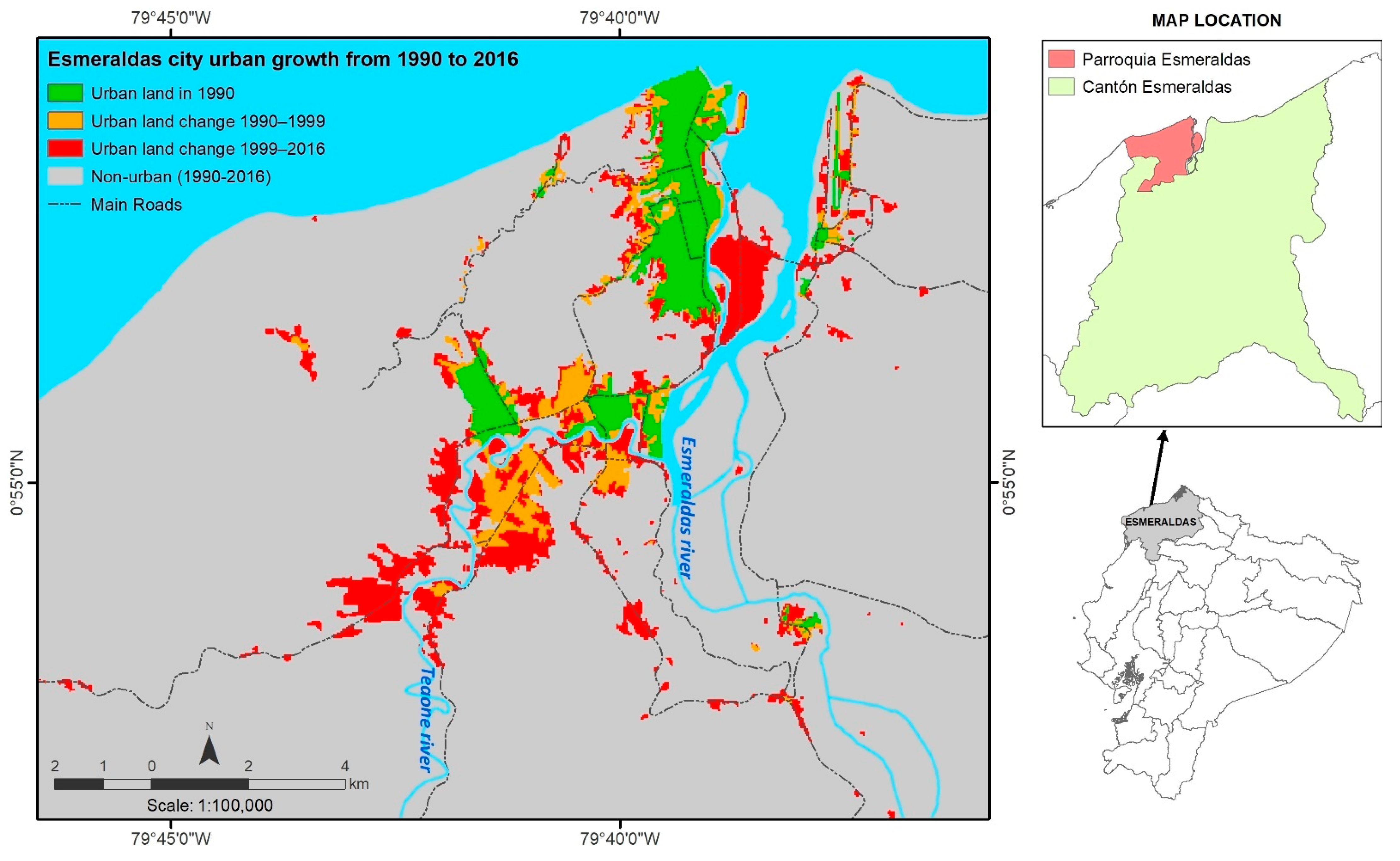
1.1. Esmeraldas City: Regional and Local Context

Located in the northwestern corner of the country (see Figure 1), Esmeraldas is one of the poorest provinces in Ecuador [29], with a long history of segregation and exploitation of its natural resources [30,31]. Due to its location in the Choco bio-geographical region—known for having one of the highest biodiversity rates in the world [32,33]—a long history of natural resource extraction is associated with the region. Additionally, in the last few decades, the city’s proximity to Colombia’s coca-growing regions has had an impact on its social dynamics, resulting in high levels of urban violence and crime [34]. It has become one of the preferred destination of people escaping from violence in Colombia [35].

The city of Esmeraldas has been growing rapidly, from 100,221 to 161,868 inhabitants between 1990 and 2010 [36,37], with more than half (56.4%) of the population having an Afro-Ecuadorian background. Historically, the economic dynamics of the city have been based on enclaves prompted by external funding, such as the banana and oil industries, as well as seaport activities. These economic activities offer low-skilled jobs, and became the main rural immigration pull factors, incrementing the city’s population. Additionally, poor city planning generated urban growth based on informal settlements with no basic service coverage, and on lands vulnerable to natural hazards, becoming the structural basis for the population’s social problems (Rebotier et al., 2020). Nearly 60% of the dwellings are located in informal settlements without any form of building permits [33]. Current statistics of poverty and inequality show that 52.2% of the total inhabitants live in poverty due to unsatisfied basic needs (INEC, 2010). The secondary effects of the COVID 19 pandemic are expected to increase these levels of poverty and vulnerability.

Urban land growth is an important process that has a strong relationship with population growth, and the technical evaluation of this development process and its conditions are the basis for governments to make policies cautiously [38]. Esmeraldas’ urban land expanded from 8.59 km² in 1990 to 14.69 km² in 1999, and to 27.2 km² in 2016 (Figure 1), tripling in the last 25 years. However, this expansion in area is seriously limited by natural and economic barriers, which push low-income families to the outskirts of the town, towards areas that are prone to flooding and landslides [34,39].

Urban growth began in 1960, occupying the northern region (actual Las Palmas neighborhood) and the hillsides located in the southwest of the city. Historically, the settlements located in the western region were affected by landslides as a result of strong rainfall events during the wet season [34]. The current configuration of the city emerged in the mid-1970s with the construction of landfills over the left margin of the Esmeraldas River [40,41], due to a strategic location that benefits trade, industry, and economic development. In consequence, this brought about the deforestation of about 42 hectares of mangrove forest [40], which resulted in increased flood exposure in new settlements. The presence of the oil refinery also shaped the expansion of the city towards the southeastern areas, prompting an increase in workforce settlements for its operation in high-risk sites and with no planning guidelines [39].

1.2. Urban Vulnerability in Esmeraldas

Esmeraldas is a coastal city exposed to the impacts of naturally induced disasters, including sea-level rise, flooding, and landslides with their related effects [42,43]. However, extreme levels of poverty and a low capacity to adapt to climate change make it even more vulnerable to natural hazards and their consequences. El Niño and La Niña are examples of such events that have had a great impact on the climate, mainly in the Ecuadorian Coast. Both are opposite effects of the same phenomenon, now known as the El Niño Southern Oscillation (ENSO), characterized by an anomalous and widespread warming of central and eastern tropical Pacific Ocean sea surface temperatures [44]. Esmeraldas is located at the extreme north of the ENSO events influence area, and has experienced important economic losses in the past two decades, which are related to the overflowing of rivers and landslides due to intense precipitation [45]. In recent research, Fasullo et al. [46] created and ran a multiple model to see how ENSO’s impacts on temperature and wildfire probability will change in a warmer future world, concluding that these impacts will be more extreme.

Esmeraldas’ climate is classified in the semi-humid megathermal tropical category, characterized by an average temperature ranging from 25 °C to 26.2 °C and a relative humidity of 81% [47,48]. It is also influenced by the warm, low-salinity estuarine waters of the Esmeraldas River system, one of the largest rivers of the region [49]. Based on meteorological measurements (1981–2017), the average annual precipitation in Esmeraldas is about 1000 ± 177 mm/year, where heavy rainfall has been correlated with El Niño occurrences (Figure 2a). In the last decade, this value has increased to 1437.20 ± 432 mm/year, evidencing the increased frequency of extreme El Niño events [50,51].

In the city, precipitation is not evenly distributed during the year, with 80% of the annual rainfall occurring from December to May (Figure 2b). In the wet season, the maximum rainfalls occur in January and February, with an average mean precipitation of 200 mm. The 1997–1998 ENSO event was a period wherein the precipitation was over 100 mm/month, even in the dry season, resulting in a total precipitation of 3739.8 mm for the July 1997–June 1998 period. The El Niño event experienced during 1997–1998 was considered as very damaging to the infrastructure of Esmeraldas, affecting infrastructure and livelihoods, including agriculture, fisheries, and industry [52,53]. The city’s dwelling units have also been affected by an increased frequency of flooding and landslides [53].

2. Dataset and Data Preprocessing

The basic data land use/cover maps were extracted from Landsat satellite images acquired on 21 February 1990, 3 April 1999, and 3 May 2016 of the Path11/Row59 scene. Pre-processing procedures were performed in order to transform raw sensor data (Digital Number) into surface reflectance data using the ENVI software. These images were geo-rectified with a 2016 scene as reference. Seven land use classes—soil, forest, shrub vegetation, pasture, crops, urban land, and water—were extracted applying an object-based classification method. The first five classes are considered non-urban areas that have potential for urbanization, and the water class is considered as not suitable for development and was therefore considered as a constraint and excluded from future analysis.

The 1999 land use/cover map was used to produce the model’s initial urban pattern, while the 2016 map was used to generate its final urban pattern. These maps were reclassified in two categories and set as binary data, with 1 representing urban land and 0 representing non-urban land. These maps were used to calibrate the CA model considering the acquisition date of the explanatory variables.

A set of 11 potential determinants or variables (

Table 1. Summary of the key driving factors for the urban growth in Esmeraldas.

Variable	Description	Data Source
Proximity to roads	Euclidean distance from the cell to main roads	Base geographic information from Instituto Geográfico Militar (2013). Scale: 1:50,000.
Proximity to rivers	Euclidean distance from the cell to main rivers	Base geographic information from Instituto Geográfico Militar (2013). Scale: 1:50,000.
Proximity to focal points	Euclidean distance from the cell to the nearest focal point within the city: commercial, administrative and industrial sites	Base geographic information from Instituto Geográfico Militar (2013). Scale: 1:50,000.
Elevation	The elevation of the cell	Digital Elevation Model from SRTM * data (30 m, 2014)
Slope	The slope of the cell (degree)	Digital Elevation Model from SRTM * data (30 m, 2014)
Landslide	Number of landslide occurrences per square kilometer calculated in each cell. Zones where landslides are likely to occur based on historical information.	Data collected in the 2C ** Esmeraldas project (2017). Local Municipality information
Flood	Number of flood occurrences per square kilometer calculated in each cell. Zones where floods are likely to occur based on historical information.	Data collected in the 2C ** Esmeraldas project (2017). Local Municipality information.
Population density	The population density of the cell. Number of people living per square meter.	National Census data 2010 [37]
Afro-Ecuadorian fraction	The Afro-Eecuadorian fraction of the cell at census administrative level.	National Census data 2010 [37]
Poverty	The poverty rate of the cell based on the unsatisfied basic needs (infrastructure, housing conditions, sanitary conditions, education, and subsistence capacity)	National Census data 2010 [37]
Crime density	The crime density of the cell. Number of crimes (property and violent crimes) per square meter occurred in 2010.	General Operations Division Policía Nacional del Ecuador, 2010

* SRTM: Shuttle Radar Topography Mission. ** Secondary Cities Project.

) was identified in order to explain the probability of non-urban land being converted to urban land. These urban land change driving factors were derived from statistical analyses and empirical and theoretical relations among driving factors and urban growth, based on the literature [54,55].

These factors represent the spatial influence of an entity or activity (accessibility), the physical characteristics of the local land (suitability), the spatial exposure to natural hazards, and the spatial variation in socioeconomic conditions. All these variables were processed and spatialized via GIS functions. The census and police data were spatialized at administrative census level. All variables were resampled to 30 m spatial resolution to match the land use/cover maps derived from the Landsat imagery. Additionally, all variables were standardized to the 0–1 range.

3. Methods

To achieve a comprehensive analysis of the urban vulnerability in Esmeraldas, this study follows a specific process: (Section 3.1) urban growth modeling for 2030 using a CA simulation model regarding the interactions between social, physical, and environmental changes and urban growth, and (Section 3.2) analysis of vulnerability to climate change based on socioeconomic conditions and focused on flooding- and landslide-exposed areas.

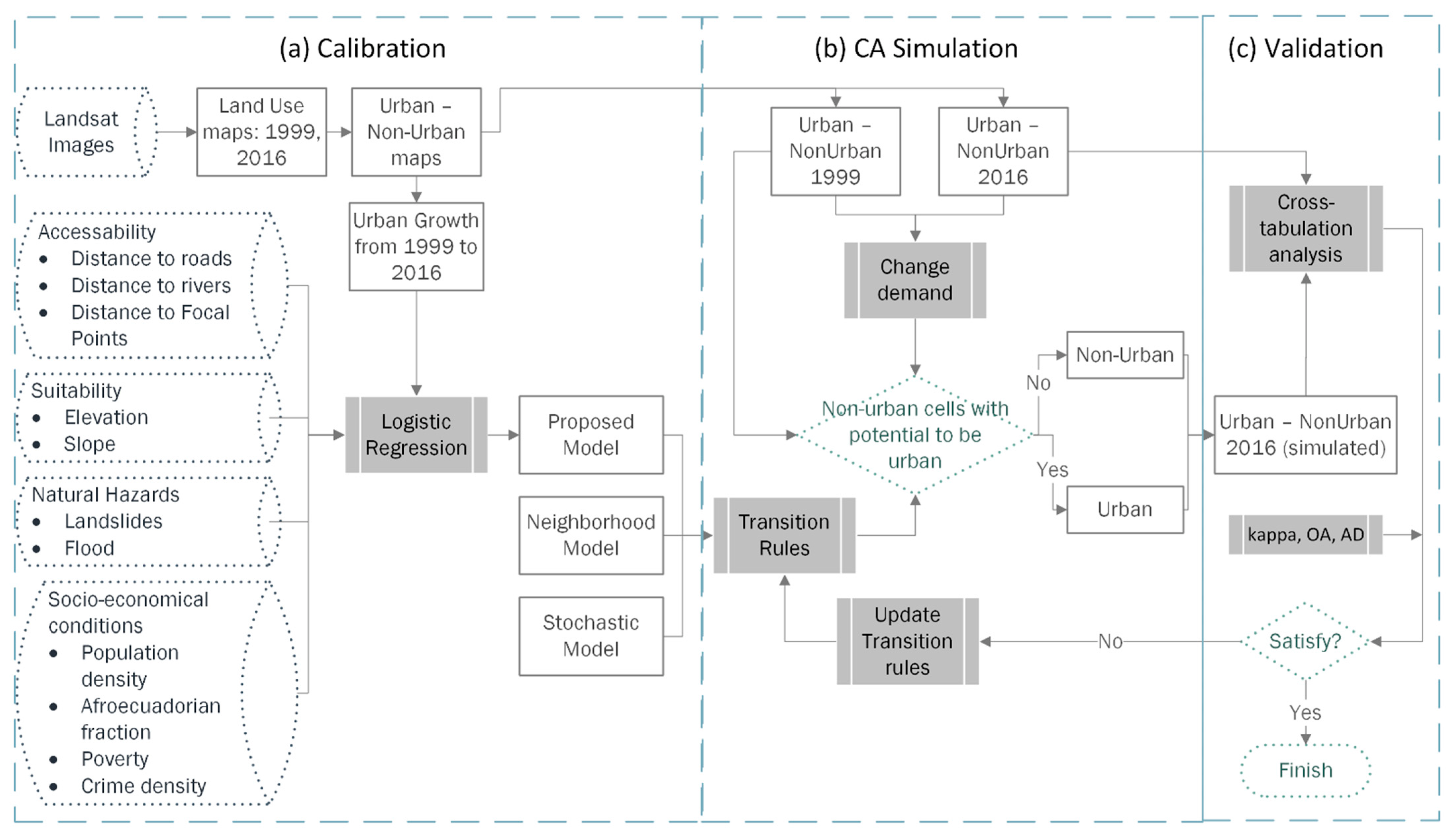
3.1. Urban Growth Model Structure

An urban growth model, based on a logistic regression model and a constrained CA model, was developed to predict urban transition probabilities in Esmeraldas. The model was developed in the free-access R software environment and consists of three main steps: calibration, simulation, and validation (Figure 3), as described in the next sections.

3.1.1. Urban Growth Calibration Model

The success of CA in urban growth simulation is the optimum determination of the CA transition rule. The use of other modeling techniques and statistical approaches in conjunction with the CA model is more useful to calibrate the urban transition rules. For this study, a conventional logistic regression was built to explore and address the spatial patterns of the drivers of urban land conversion besides eliminating spatial autocorrelation and reducing spatial dependency among variables. Logistic regression is a form of regression based on the concepts of binomial probability theory, which is used to model the relationship between a binary variable and one or more explanatory variables, yielding dichotomous outcomes.

For this model, the land use conversion from non-urban to urban was considered as state 1, while no conversion was indicated as state 0. Multi-collinearity among explanatory variables was tested using Pearson’s correlation and variance inflation factors (VIFs). The results of the analysis show there was no significant multicollinearity observed among the set of the variables in the model. All the variables scored VIF less 5, the threshold level suggested to deal with multicollinearity. Therefore, the entire set of variables was incorporated into the model.

3.1.2. CA Simulation Model

The spatially explicit simulation uses a cell-based, dynamic modeling approach based on Cellular Automata (CA) principles to calculate non-urban to urban changes in annual time steps. The SIMLANDER (simlander.wordpress.com) a simulation of land use change using R algorithm, which is a prototype Cellular Automata (CA), was implemented in this study. The original script was modified to improve the model fit in order to address the local conditions in Esmeraldas’ urban growth.

The simulation process defines the initial conditions of the system, which are represented by an initial land cover classification in year t (for this case, the urban–non-urban map of 1999). This is followed by the determination of the transition rules within the system, which allow us to produce transition potential maps. The transition potential maps indicate the ability of a pixel to turn from one state to another, or to remain unchanged [56].

To build the overall transition rule, two important parameters were included to capture the local and regional dynamic: the neighborhood factor and the stochastic factor. The neighborhood factor was built using a moving window of 5 × 5 cells (150 × 150 m), estimated from the cumulative allocated development of the previous period, where the central or focal cell is susceptible to change based on the values of its neighbors. The weigh matrix that achieves a better simulation in this study was found using a trial-and-error method. The uncertainty addressed in this study is the stochastic (random) factor, which describes the inherent variation associated with the system or the environment under consideration. A random distribution is generated in a range of [0, 1] to represent the possibility that land cover may change in less predictable ways and isolated locations; in other words, to represent the stochastic behavior using urban agents. Thus, the overall transition rule for each cell in the model was given by:

$$P{r}^{t_u}=P+\left(N\times St\right)$$

where $Pr$ is the urban land use conversion probability of a cell at time $t_u$, $P$ is the logistic regression model, $N$ is the normalized neighborhood effect, and $St$ is the normalized stochastic factor.

The annual demand for urban area was calculated from the difference between the built-up land in the final year (2016) and the built-up land in the initial year (1999), divided by the number of the years in this period. For the future simulation of urban growth in 2035, the urban demand was projected based on built-up growth rate for the 1990–1999 and 1999–2016 periods. In this context, the urban demand for the 2016–2035 period was estimated at 872 cells per year.

Finally, the urban growth model was built through the integration of all these procedures in the annual interactive CA modeling process, where, for each year, the highest potential pixels are selected and converted to urban land until the demand is filled. The CA output is a map showing a simulation of the urban growth in a known year. If the results of the simulation assess goodness-of-fit against the reference map (for this case the urban–non-urban map of 2016), the process is completed and the transition rule is accepted for future simulations—in this case for the year 2035. Otherwise, it is necessary to apply modifications to the transition rule, and then the above process is repeated until the resulting map is made satisfactory through the validation process.

3.1.3. Model Validation

The accuracy of the simulation results compared to the reference map needs to be validated to quantify the goodness-of-fit. A cross-tabulation analysis was used to compare the simulated map and the reference map, wherein four generalization types of pixels are summarized: areas of observed urban change simulated correctly (hits; H), observed non-urban simulated as urban (false alarms; F), observed urban change simulated as non-urban (misses; M), and observed non-urban simulated as non-urban (correct rejections; CR) [11]. Derived from the cross-tabulation analysis, the overall kappa index (K), overall accuracy (OA), and the allocation disagreement (AD) are presented to assess the accuracy of the model.

3.2. Vulnerability to Climate Change

Based on the predictive scenario of Esmeraldas’ urban growth for 2035, a vulnerability analysis was implemented with a focus on landslides and flooding risks, given its current level of exposure. These events are generally triggered by high-intensity rainfall [57] and the increased precipitation could cause additional life and property loses [33].

Thus, future precipitation variability for the 2016–2035 period was examined using downscaled projections, which allowed us to understand the potential impacts of climate change over Esmeraldas’ urban land. These projections, provided by the Ecuadorian Ministry of Environment’s (MAE for its acronym in Spanish) official estimates, consist of the dynamically downscaled outputs of four Global Circulation Models (GCMs): CSIRO-Mk3-6-0, GISS-E2-R, IPSL-CM5A-MR, and MIROC-ESM. The final spatial resolution of this multi-model is 10 km, and it was built under two scenarios: RCP4.5 and RCP8.5. Climate conditions were characterized for the 1981–2015 reference period.

Additionally, the use of scenarios defined by impact thresholds (elevation and slope) that consider physical vulnerability reported by scientific data was helpful to effectively assess the degree of population susceptibility at the regional scale. For flooding vulnerability scenarios, the Fifth Assessment Report of the IPCC suggests that mean sea levels could rise by 1 m or more by 2100 [58], which will have severe impacts on costal environments. According to the Fourth National Climate assessment [59], the IPCC projects are still somewhat conservative, and do not reflect the full range of physically plausible global average sea-level rise (SLR) over the 21st century. Recent studies suggest that global SLR could exceed 2.5 m by 2100 considering a business-as-usual scenario [60,61,62]. Based on these estimates, and considering short-term climate change, the flood risk was spatialized with a 1.5 m of sea-level rise scenario calculated by the SRTM (Shuttle Radar Topography Mission), identifying impacted areas of actual urban land and the predicted urban growth for 2035.

Landslide vulnerability is based on the local terrain condition, wherein the slope angle is an active parameter directly related to the physical proprieties and the formation of landslides, and it is the most influential and essential factor in landslide susceptibility [63,64]. Some studies suggest that slope gradients between 30° and 45° are susceptible to mass movement, while others believe it can occur above 25° [63,65]. This situation could vary regionally, and could be influenced by external parameters such as wind and rainfall. Heavy rainfall and an excess amount of groundwater could affect the stability of slopes between 5–15°. Thus, this study evaluated landslide risk with moderate slope angle values, spatializing a scenario with slopes above 25 degrees to identify the actual and predicted urban land impacted by mass movements.

Finally, we have characterized the socioeconomic composition of the city, identifying critical weak points in the settlements that are currently exposed to landslides and flooding hazards based on an urban land map for 2016. This evaluation used the National Census data [37] to characterize the “census sectors” with a high vulnerability to climate events and natural risks. The features that were considered in the analysis include dwelling conditions and living standards, socioeconomic characteristics, and demographic features.

4. Results

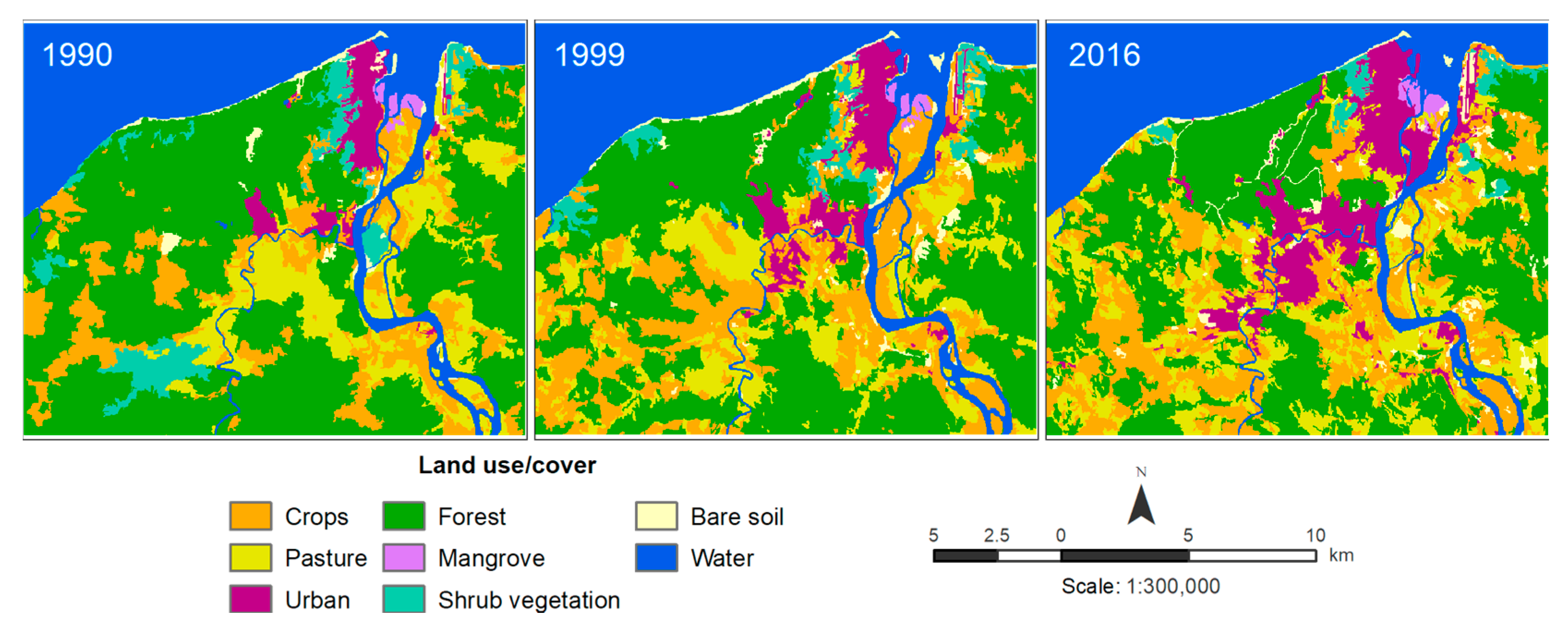
4.1. Land Use and Land Cover Mapping

It was found that the actual urban land increased from 8.6 km² to 27.2 km² during the period 1990–2016, with an increase of 6% in total area (

Table 2. Land use/land cover area (in square kilometers) statistics for 1990–2016.

	Bare Soil		Forest		Urban		Shrub Vegetation		Pasture		Mangrove		Crops
	km2	%	km2	%	km2	%	km2	%	km2	%	km2	%	km2	%
1990	4.1	1.3%	145.4	45.7%	8.6	2.7%	14.4	4.5%	34.5	10.9%	1.3	0.4%	39.5	12.4%
1999	6.6	2.1%	118.1	37.1%	14.7	4.6%	9.2	2.9%	37.9	11.9%	1.1	0.3%	60.4	19.0%
2016	7.9	2.5%	100.2	31.5%	27.2	8.6%	4.9	1.5%	48.4	15.2%	1.4	0.4%	58.6	18.4%
1990–2016 (Δ%)		1.2%		−14.2%		5.9%		−3.0%		4.4%		0.0%		6.0%

). Periodic observations show that the built-up area increased 6.1 km² in 1999, mainly concentrated in the central region, which later increased by 12.5 km² in 2016, continuing with an expansion over the central and southern regions (Figure 4), primarily along the Teaone and Esmeraldas Rivers, and on the Piedad and Prado Islands located in the northeastern region.

In contrast, the overall change in vegetation area (forest and shrubs) from 1990 to 2016 was observed to be −17.2%. The forest cover occupied 145.4 km² (45.7%) in 1990, which decreased to about 100.2 km² (31.5%) in 2016, mainly replaced by agricultural activities. Shrub vegetation, concentrated on the hillside west of the city in 1990, decreased from 14.4 km² to 4.9 km², with a −3% change, primarily resulting from urban expansion. The area covered by mangroves showed a slight change in the period, from 1.3 km² to 1.4 km²; however, its spatial configuration was impacted by river dynamics and human influence. Mangrove forests play an important role in the local population’s adaptation to climate change [66,67], but the mangroves that are located in this area are the last remains of an extensive forest that was transformed by urban development and by the encroachment of agricultural and aquaculture activities. All the agricultural land (pastures and crops) covered a total area of 74.0 km² (23.3%) in 1990, which increased to 107 km² (33.6% of the total area) in 2016.

4.2. Urban Growth Modeling

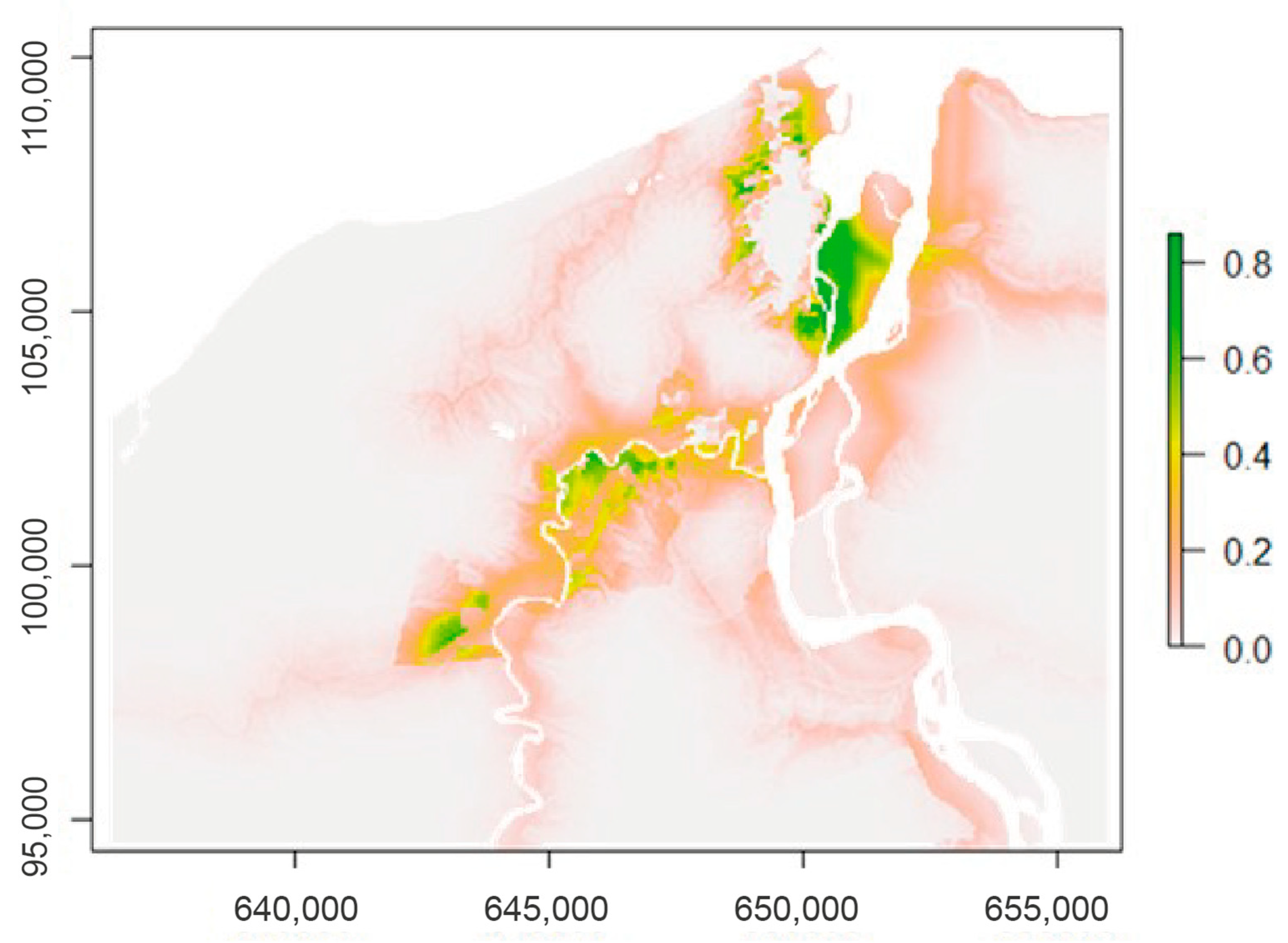
4.2.1. Model Calibration: Transition Rule

The key factors responsible for the changing patterns of urban growth are presented through the binary logistic regression results shown in

Table 3. Estimated coefficients and odds ratios for the logistic regression model of 1999–2016.

	Coefficient	Std. Error	p-Value	Odds Ratio
Intercept	−1.13	0.05	0.000 *	-
Proximity to roads	−19.93	0.35	0.000 *	2.20 × 10−9
Proximity to rivers	−1.07	0.10	0.000 *	0.344
Proximity to focal points	−3.08	0.07	0.000 *	0.045
Elevation	−0.47	0.11	0.000 *	0.625
Slope	−3.45	0.17	0.000 *	0.031
Landslide	2.39	0.07	0.000 *	10.937
Flood	1.84	0.05	0.000 *	6.303
Population density	−2.28	0.15	0.000 *	0.101
Afro-Ecuadorian fraction	2.76	0.06	0.000 *	15.930
Poverty	−0.95	0.04	0.000 *	0.386
Crime density	−156.46	4.9	0.000 *	1.116 × 10−68

α = Significance level, * α = 0.001.

. All the variables are significant at α < 0.001. The relative significance of the explanatory variables can be concluded from the odds ratio (OR), which is an indicator of the change of odds resulting from a unit change in the predictor, and the value of coefficients of the variables obtained from the model [55,68].

The results in Table 3 show that only three variables—proportion of Afro-Ecuadorian people, landslide, and flooding—have a positive relationship with Esmeraldas’ urban growth. This means that the greater the variables’ value, the higher the probability of the land unit being urbanized. In contrast, the remaining eight variables are negatively correlated with urban growth, implying a higher urbanization probability in areas close to roads, rivers and focal points, or when the variables’ (elevation, slope, population density, poverty and crime density) values are smaller.

The odds ratio results suggest that the following factors were found to affect urban growth with varying degrees of influence for Esmeraldas (with odd ratios larger than 10 or less than 0.1): distance to roads, distance to focal points, slope, landslide-susceptible areas, population density, Afro-Ecuadorian fraction, and crime density of urban pixels. Finally, these results were used to determine the urban development suitability mapping in Esmeraldas, as shown in Figure 5. The values range from 0 to 1, where the green tones indicate higher probabilities of urban expansion. The future pattern of urban expansion is easy to identify from this map, and an urban development potential is observed in the southwestern and northeastern parts of Esmeraldas City, regions where the oil industry and the terrestrial and aerial transport services are located.

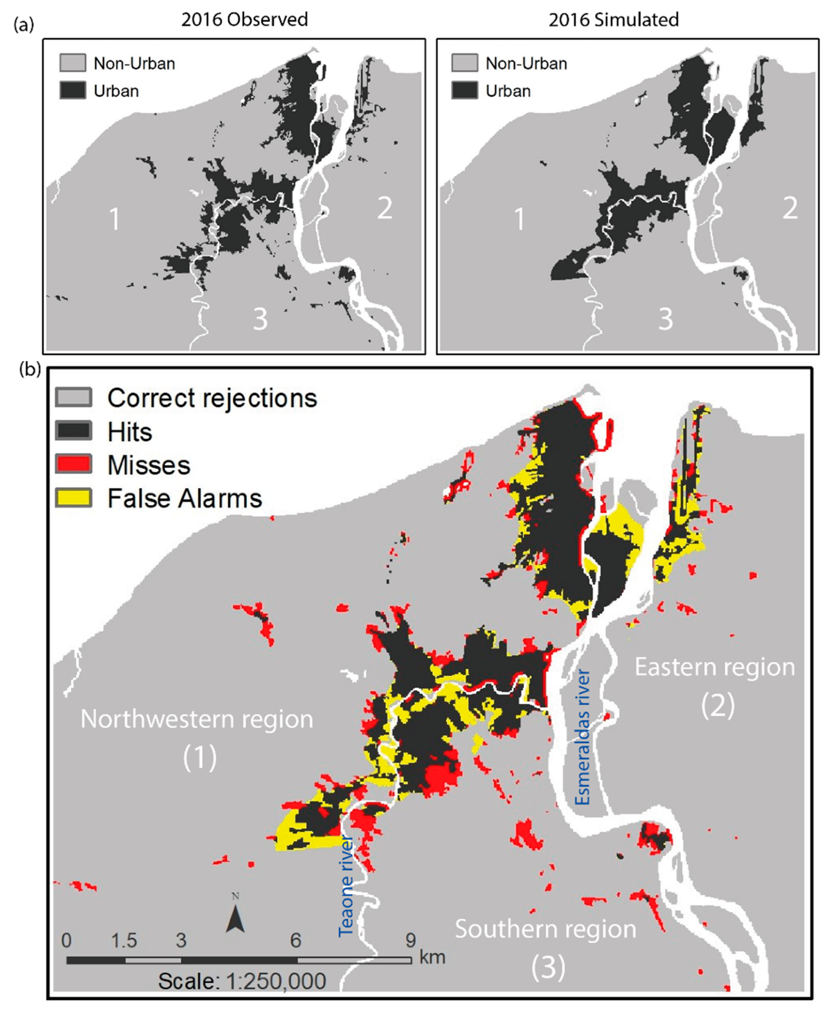
4.2.2. Model Simulation and Validation

The proposed CA model for simulating the urban growth in Esmeraldas for the year 2016—using 1999 as a baseline year—was implemented, and the model’s results are shown in Figure 6. The study area was divided into three regions (for visual analysis only) delimited by the main rivers that flow through the city: northwestern region (1), eastern region (2), and southern region (3). Visually, the simulated patterns fit better with the actual (observed) urban patterns for 2016 in region 1 than the results from the other regions (Figure 6a). The main noticeable differences in regions 2 and 3 are that the simulation shows a lower predicted growth in the southeast part of region 3, and a somewhat less fragmented urban land pattern in region 2 and the northern part of region 3.

The distribution of allocation errors (missed and false alarms) in the CA model results is illustrated in Figure 6b. The figure reveals that the model correctly simulates a larger area of actual urban growth (black) in regions 1 and 3 than in region 2. Missed (red) and false alarm (yellow) areas are relatively small in region 1, while the yellow and red areas are relatively larger in regions 2 and 3, respectively. This could be attributed to the administrative division in the rural areas located in these regions, where the division’s area is greater than in urban zones. This administrative division (“Sector Censal”) is based on population density.

For model accuracy assessment, the real and the simulated maps were used to validate the model’s capabilities in producing simulation results.

Table 4. Cross-tabulation analysis of the CA model, number of pixels, and the percentage in parenthesis.

Simulation		Urban	Non-Urban	TOTAL
	Urban	23,356 (6%)	6758 (2%)	30,114 (8%)
	Non-urban	6757 (2%)	318,449 (90%)	325,207 (92%)
	TOTAL	30,113 (8%)	325,207 (92%)	355,320 (100%)

shows the tabular matrix resulting from the cross-tabulation analysis. It represents the proportion of pixels in the 2016 observed map versus the simulated map, illustrating the allocation disagreement between the simulated and observed changes. The overall kappa, overall accuracy, and the allocation disagreement of the CA model were 76%, 96%, and 4%, respectively, indicating a high level of consistency between the simulation and reality.

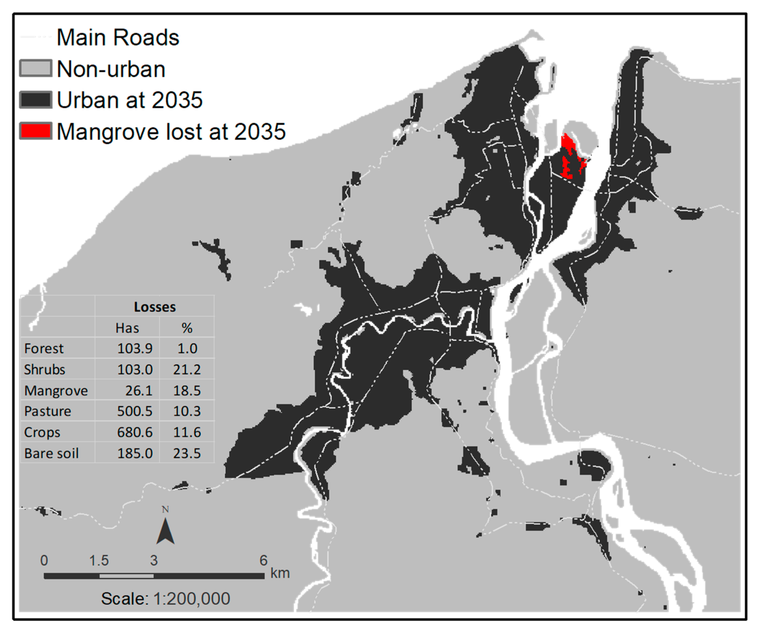
4.2.3. Urban Growth in Esmeraldas for 2035

After the validation process, the proposed CA model was applied to predict the future urbanization in Esmeraldas City for the year 2035, as is shown in Figure 7. The simulation presented in this study reveals the city’s tendency to expand into bordering areas, and in proximity to main roads and rivers. Based on the projected model, the urban growth area in Esmeraldas will be 16 km², making a total of 43.1 km² of urban land in 2035, meaning an increase of 50% compared with the year 2016.

Considering the actual land use in the study area, the projected expansion of urban land in 2035 would be accompanied by an important decline in native vegetation (loss of 40.7%), followed by bare soil (loss of 23.5%) and agricultural land areas (loss of 22%). This pattern threatens ecosystem services in the area, and the conservation and integrity of the native ecosystems will be heavily affected. Additionally, the projected model shows that 26.1 ha of mangrove forest will be removed by 2035 due to urban growth (red area in Figure 7), increasing at almost twice the annual rate of loss (1.28%). If the present rate of loss continues (1 to 2% a year), ecosystem goods and services, such as flood defense, could be lost by 2035 [51,66].

4.3. Urban Exposure to Climate Change

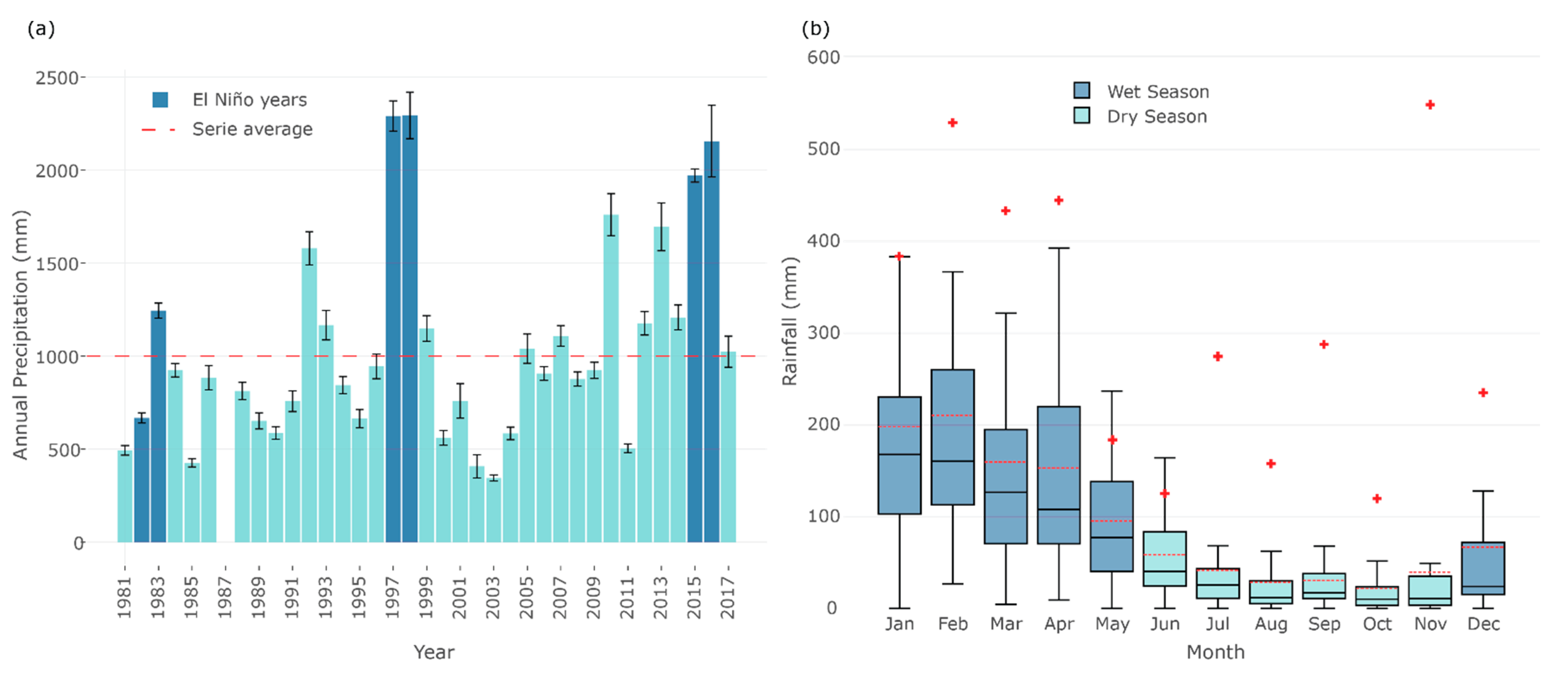
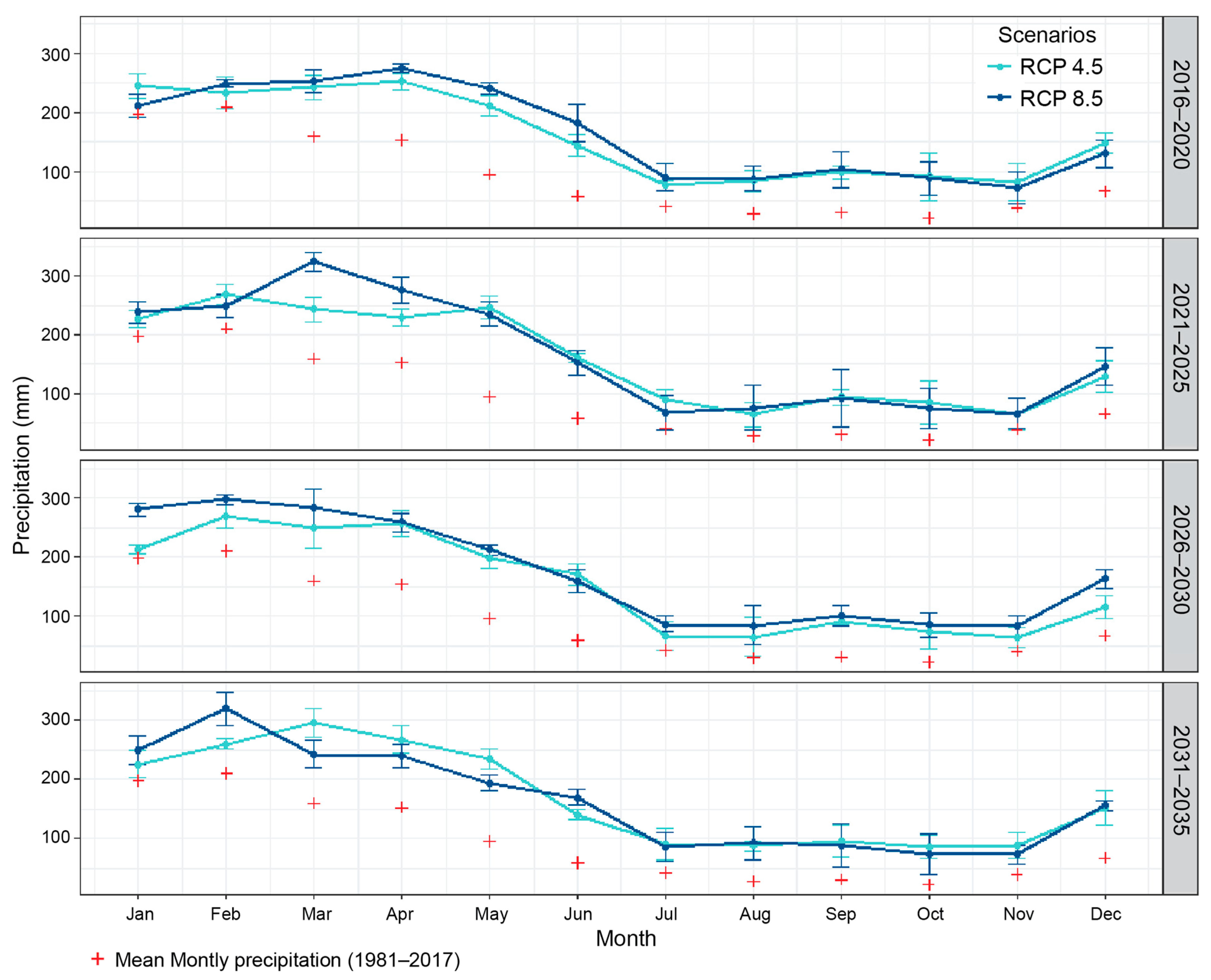
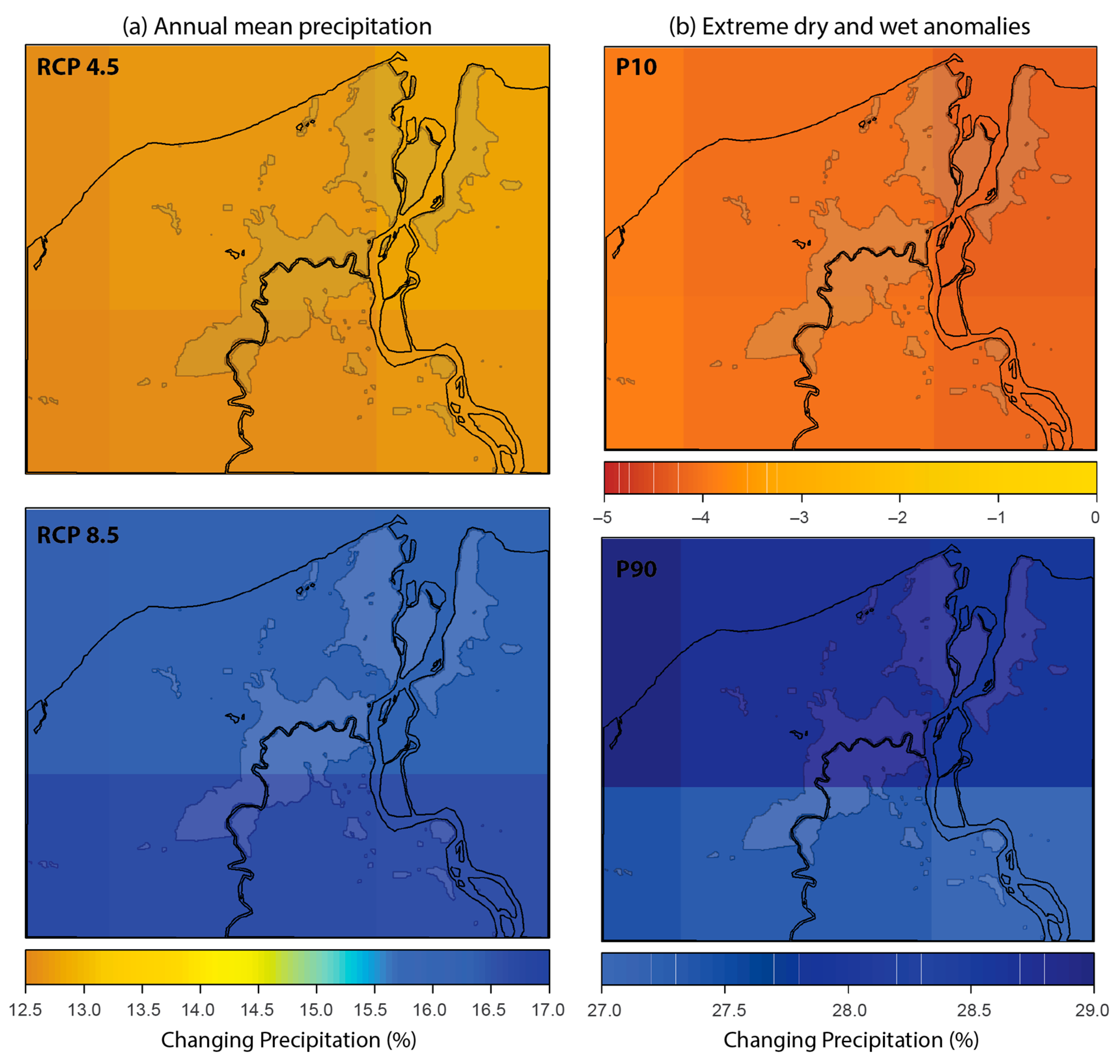
4.3.1. Future Precipitation

By examining the trends of future rainfall in Esmeraldas, derived from the MAE climatological repository, we can see a notable increase in precipitation over the 2016–2035 period when compared with the historical reference period of 1981–2017 (Figure 8), suggesting a future wetting condition in the city. The projected monthly rainfall, particularly its magnitude, differs across the scenarios and time period (5 years) mainly in the wet season. Conservative estimations (RCP 4.5) project a monthly rainfall that ranges from 200 mm to 250 mm between January and May, while for most extreme climate projections (RCP 8.5), it ranges from 250 mm to 300 mm in the same period. These results show an intensification of the wet season with an increase in the number of months with precipitation over 200 mm.

Furthermore, projections show that the maximum precipitation occurs in February and March under the RCP 8.5 scenario, with monthly cumulative rainfalls over 300 mm in the 2021–2025 and 2031–2035 periods, which could be due to the influence of future ENSO events in these periods.

The projected changes show that multi-model mean annual precipitation would increase by between 12.5% and 17% across the city by 2030 (Figure 9a); however, future spatial patterns differ across scenarios. Conservative climate estimations (RCP 4.5) suggest a wetter future in the northeastern region, while extreme estimations (RCP 8.5) project higher precipitation over the southwestern region. Changes in extreme conditions (Figure 9b) indicate that for extreme dry anomalies (10th percentile), the low precipitations may not change significantly (percent changes between −5% and −3%). As for extreme wet conditions (90th percentile), rainfall may increase by about 28%. Additionally, we note that the northeastern part of the city may be affected by extreme conditions. We acknowledge the need to improve local climate observations and projections that include temperature records and hydrological variables, yet here, we expect to show an initial overview of the rainfall conditions.

Considering urban growth and its exposure to heavy rainfalls, the spatial patterns indicate that the northeastern and southwestern regions, where much of the future urban growth is expected to take place, will receive more rainfall than the other regions. The high rainfall in these areas is expected to worsen the flood situation along the Esmeraldas and Teaone Rivers, meaning extensive land losses in the immediate surrounding area by the 2030s, as well as significant economic and human impacts.

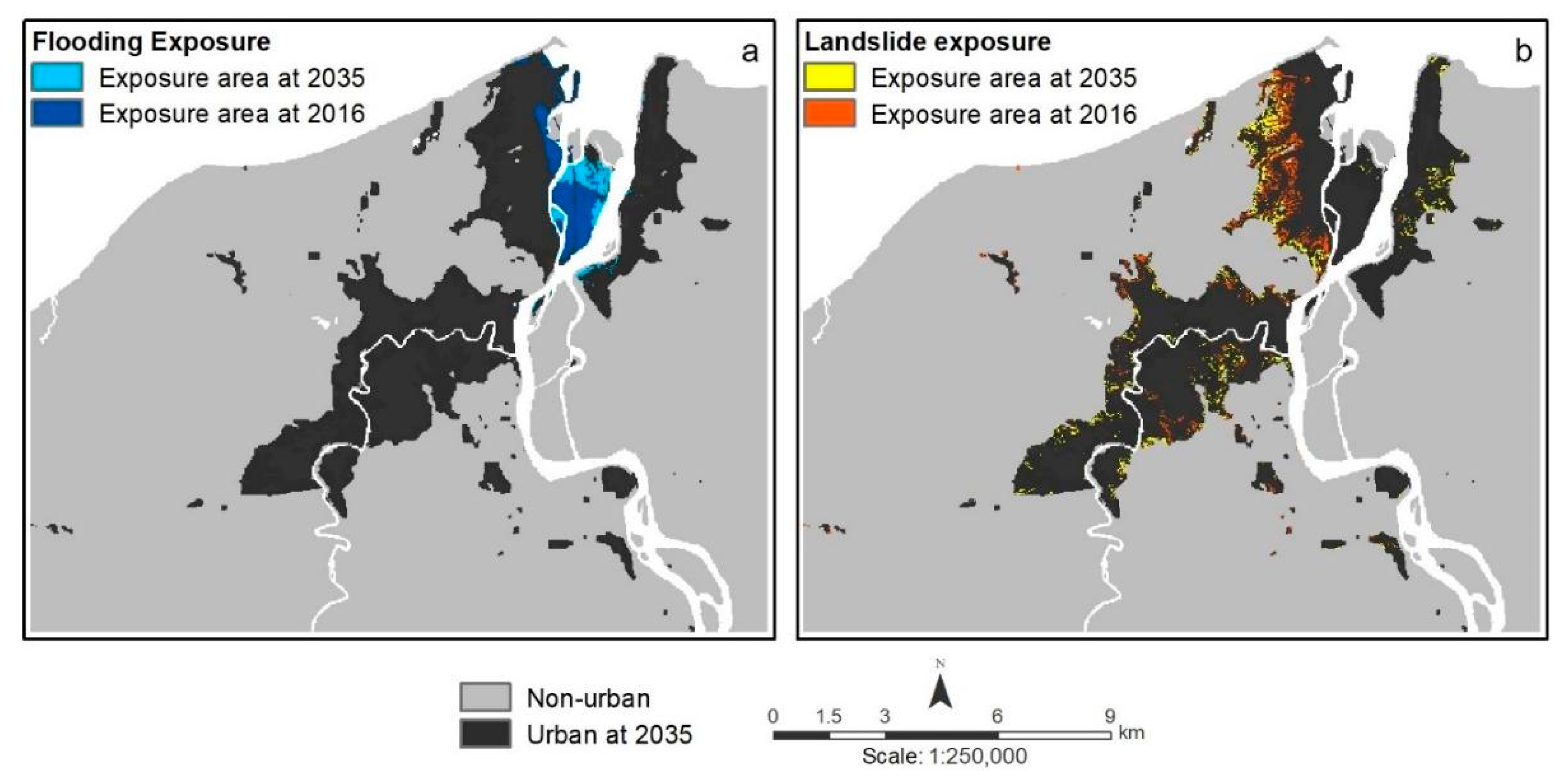
4.3.2. Exposure Scenarios

Analyzing the present and future projection of urban growth development in this study, we found that 240.39 ha (9%) of the Esmeraldas urban area was exposed to 1.5 m of sea level rise in 2016. By 2035, this value will have increased in 91.35 ha of exposed urban area, to a total of 331.74 ha (Figure 10a), which represents 8% of the total urban land for this year.

As for landslide risk, based on the 2016 urban map, houses on hills of over 25 degrees are built in over 156.36 ha (6%) of the land. The projected model indicates that this area will increase to 337.26 ha (8%) by 2035, and these new settlements will suffer the risk of landslides (Figure 10b).

Overall, about 15% of the urban land was exposed to the effects of climate variability in the year 2016. Two decades later, the existing tendency of the population to build on areas highly exposed to climate-related risk will continue (16% of the urban land will be exposed to climate change effects).

4.3.3. Population Vulnerability

Imran et al. (2019) considered that social vulnerability due to natural hazards is driven by socioeconomic conditions, demographics, status of land tenure, coping capacity, and spatial neighborhood (e.g., road networks, housing quality, connectivity of flood-prone communities), and that the interrelationships between these constructs reveal reinforcing dynamics between them. The values of the parameters selected for analyzing the socioeconomic condition of the population that has settled on flooding- or landslide-vulnerable areas are presented in

Table 5. Housing conditions and population characteristics of settlements located in flooding and landslide exposure areas, and in non-vulnerable areas. The values are presented in percentages.

Subject	Indicator	Values	Flooding	Landslide	No Exposure to Flooding/Landslide
Housing conditions and standard of living	Structural dwelling condition (wall, floor, ceilings)	Good	32.85	40.08	50.05
		Regular and poor	67.15	59.92	49.95
	Solid waste disposal	Solid waste collected	93.55	94.58	98
		Throwing out	2.09	0.92	0.4
		Burning or burying	4.36	4.51	1.6
	Sewage disposal	Public server	60.97	67	78.67
		Septic tank or cesspit	22.13	25.89	17.77
		Discharge into water bodies	5.52	0.78	0.54
		Latrine	0.63	0.64	0.37
		Non-existing	10.76	5.68	2.66
	Water supply system	Public system (piped system)	91.7	92.97	96.31
		Well water	1.11	1.57	0.67
		Rivers, springs	3.5	0.69	0.68
		Tanker truck	1.16	2.6	0.99
		Other sources	2.53	2.17	1.37
	Electricity system	Public service	89.14	93.82	96.4
		Solar panel	0.49	0.22	0.18
		Generator	0.63	0.19	0.16
		Other sources	2.64	1.59	0.86
		Non-existing	7.1	4.17	2.4
Socioeconomic characteristics	Education status	Primary and secondary	83.32	76.48	71.95
		Bachelor´s degree	10.26	16.55	21.41
		Post-graduate degree	0.53	1.01	1.58
		No answer	5.9	5.97	5.05
	Source of income	Government or private job	40.01	50.96	52.97
		Day laborer	7.61	5.35	4.13
		Housemaid	6.82	6.21	3.82
		Business owner	26.85	22.44	25.60
		No income	18.71	15.05	13.48
	House ownership	Owned housing	62.98	68.79	72.13
		Borrowed housing	13.35	13.9	0
		Rented housing	23.67	17.31	27.87
	Social security	Included	10.45	16.75	21.84
		Excluded	78.27	71.74	68.75
Demographic Features	Afro-Ecuadorian fraction		73.53	59.91	50.79
	Literacy rate		6.6	4.13	5.28
	Infants and children fraction		36.2	33.06	31.58
	Old age fraction		4.5	5.28	5.73
	Poverty (UBN)		59.80	50.70	39.80
	Inhabitants/Esmeraldas population		14.29	29.46	56.24

. The results show that 43.75% of the city’s population is located in risk zones, 29.46% of which is located in landslide exposure areas and 14.3% in flooding-vulnerable areas.

In general, the socioeconomic parameters show lower percentages in dwelling conditions, basic services coverage, education status, and social security access, and higher levels in illiteracy rate, than the ones presented in the areas of the city that are not exposed to flooding and landslides. However, the population that lives in areas exposed to flooding stand out due to evident precarious conditions. The population that lives in dwelling units in regular or poor conditions are 17.20 points higher than in those areas with no exposition. Additionally, sewage disposal and electrical service coverage are significantly lower than the in rest of the city, thus the proximity to the river makes it easier to fill the gaps in access to basic services, such as water supply, sewage disposal, and solid waste disposal.

As for the educational characteristics, in flooded zones, 11.37% less of the population only achieved elementary and high school education, compared with the non-vulnerable city areas. Furthermore, the proportion of people that achieve a bachelor or professional degree is between 40 and 50% less. The literacy rate in flooded plain settlements is higher (6.6%) compared with the population that lives in landslide-exposed (4.1%) and non-exposed areas (5.3%).

The Afro-Ecuadorian fraction located in flooded zones is 31% higher than in the rest of the areas, and in proportion, almost 50% fewer people in this area receive social security benefits. As for the poverty level, based on unsatisfied basic need (UBN), more than 50% of the population that lives in areas exposed to climate change hazards is considered poor, so it is necessary to concentrate mitigation efforts in these areas.

5. Discussion

The effects of climate change on society are not only a function of exposure to temperature and precipitation changes, or increases in the frequency or magnitude of extreme events. The sensitivity and adaptive capacity of societies to these changes play a crucial role in influencing outcomes [13]. In this regard, current studies have shown that socioeconomic development will largely influence future trends in social vulnerability to climate hazards [69]. It is also recognized how important these comprehensive future dynamics of human systems are, and the influence they will have on future vulnerability research [70].

This study encompasses urban growth modeling (1999–2035), and its potential vulnerability to environmental hazards results from a range of social, economic, historical, and climatic factors. While enhancing adaptation to climate change has played an important role in research and policy agendas, it is essential to ask as well why some communities and people are disproportionately exposed to—and affected by—climate threats [71,72]. Thus, the use of multilevel factors (demography, economic development, urbanization, and climate) in urban modeling allows for a better understanding of the heterogeneity of the complex urban growth process (non-stationary), and the mechanisms by which these factors influence urban expansion [22,73] and contribute in generating future impacts [13].

According to the study, future urban development is expected to occur in proximity to major roads and rivers and in low-lying lands, preferring areas close to central industry/business zones, which facilitates the mobilization of goods and people, and the access to basic social and cultural services provided by local government. However, much of this urban development process is unplanned, and the physical characteristics of these areas are not suitable for future urban sprawl. For example, in the last decade, new roads have been opened into the mangrove islands in front of the city at Isla Piedad and Isla Prado, including a bridge that links the city to the airport on the other side of the Esmeraldas River [33], giving rise to new informal settlements in these zones. These unmanaged settlement patterns reduce the sensitive and adaptive capacities of the communities facing climate change, leading to land fragmentation and pressure on land resources [56].

Socioeconomic and demographic characteristics play an important role in driving urban growth and social vulnerability to risk events in Esmeraldas. Socioeconomic, demographic, and land tenure indicators in the areas exposed to flooding and landslides reveal a cyclical vulnerability that is reinforced by the lack of urban planning in the city. Rebotier et al. [39] speak of an absence of planning rather than a failure to comply; thus, this vacuum has contributed to transforming the economic milestones, such as the banana industry, the port, and the oil industry, into dominant actors and engineers of the city’s urban structure. Hence, the population tries its best to meet its needs for housing, equipment, and services on its own, while the State intervenes by financing infrastructure for the productive economy [39].

Most of the dwellers who settle in Esmeraldas’ neighborhoods that are at risk of flooding and landslides are the result of the exponential growth of informal settlements. Mostly low-income families take part in this process, because the price of the land—when it is paid—is lower than in non-vulnerable areas. Additionally, the municipality is part of these dynamics, promoting relocations from one risk zone to another due to hazardous events that have taken place. In this context, the ownership of housing in these areas is lower than in the rest of the city, which presents a limitation to people affected by a hazardous event. This happens because land ownership promotes preventive measures and reduces damages, increasing coping capacity [74], and also because it allows claims for post-disaster government assistance.

Consequently, the levels of poverty (UBN) in Esmeraldas City clearly show that the dwellers who settle in areas exposed to flooding and landslides are significantly poorer than those in the rest of the city, with low education levels and low access to formal jobs that guarantee social security. It is also evident that households in these areas show precarious dwelling conditions and lower levels of basic service coverage, which increase social vulnerabilities because a house built with better materials and that is in good condition will be less vulnerable to a hazardous event [75], and because inadequate storm drains, waste management, and water supplies are considered some of the worst problems during a hazard, as they can significantly exacerbate the impacts during and after the event [76].

The described social scenario supports geography of exposure theories, whereby the poor tend to occupy the more risk-prone environments [16,77]. In urban areas, exposure to hazard events such as flooding and landslides tends to be concentrated in marginal, low-lying sites along rivers, on floodplains and coastal marshes, and on steeply sloping areas, which have been historically avoided by the better-off but are often settled by the poorest communities because of their availability and/or proximity to sources of economic livelihood, low prices, and less danger of eviction by city authorities (if located in areas deemed undesirable for legal private or public development) [78]. In turn, the unsustainable settlement of such areas can accentuate flooding levels and landslide risks, causing a cyclical increase in hazard exposure [77].

These social and geographical conditions state that it is not just that the poor may be more exposed to flooding and landslides, but more importantly, they are also more likely than the wealthy to suffer when flooding occurs [78]. In Esmeraldas, city dwellers in exposed areas have fewer resources upon which to draw to counteract the impacts [33]. Thus, social susceptibility becomes cyclical, because disruption to assets and livelihoods by one event often makes households even more vulnerable to future hazardous events, reflecting a loop structure whereby household losses due to one event increase their vulnerability to the next event [79].

The use of spatially explicit methodologies, such as the logistic Cellular Automata model, allowed us to explore different scenarios that conceal the complex mechanisms and processes involved in urban growth [22]. Analyzing these scenarios in conjunction with global climate downscaling models has allowed us to visualize and quantify future climate vulnerability, from both social and natural risk perspectives. These results are important assets to the Esmeraldas City authorities’ decision-making in urban land planning and management. However, further research is still needed into local climate modeling to understand the real impacts of climate change, addressing social vulnerabilities with tangible and practical knowledge.

6. Conclusions

Urban development is a complex dynamic process, whereby the population is not uniformly vulnerable to social and environmental hazards derived from climate change. The integration of multi-level factors into urban growth modeling, focused not only on accessibility and suitability parameters but also on socioeconomic and demographic characteristics, allows for a better understanding of the continuous urban development process in terms of future climate hazards. A CA logistic regression model was used to simulate and predict urban growth for 2035 in Esmeraldas City. Rainfall predictions, derived from national downscaling projections, were used to provide an understanding of future climatic conditions and their potential effects over current and future urban land. The results of rainfall projections suggest a noticeable increase in precipitation (between 12.5 and 17%) during the 2030s compared to the historical long-term average, increasing the total amount of water bodies, particularly during the wet season. The results of the model indicate that urban land in Esmeraldas is expected to increase 16 km² (50% compared to 2016) by 2035, with a notable sprawl in the southwestern and northeastern regions. Urban expansion in the city is closely associated with a significant decline in natural vegetation, led by informal settlements in high-risk exposure areas. In total, 15% of the urban land was exposed to landslides and flooding events in 2016, but a slight increase (16%) will be observed by 2035, showing a continuous marked trend towards building up in these areas.

Climate change’s effects on society depend not only on climate variability or the intensity of extreme events, but also on the sensitive and adaptive capacity of societies to cope with natural disasters. These parameters are associated with the socioeconomic and demographic characteristics of a community [80]. In Esmeraldas, this analysis reveals a high degree of vulnerability in the population located across natural risk-exposed areas, a product of informal settlements and the lack of urban planning in the city. Overall, mostly low-income families take part of this urban growth and sprawl process, whose members present low education levels and little access to formal jobs that guarantee social security. This pattern has become cyclical in Esmeraldas, reducing the resilience and adaptive capacity of households.

This study provides the basis for the prioritization of initiatives to be taken to build resilience in Esmeraldas’ population under climate change, where urban growth is primarily haphazard and unplanned. The results show a potential future damaged urban area; however, this does not mean that all the identified area will be exposed to natural hazards derived from climate change. The preparation of planning policies, a careful urban land management approach, and the identification and application of mitigation/adaptation strategies could make the results differ.

References

1. UNDESA. World Social Report 2021: Reconsidering Rural Development; United Nations Department of Economic and Social Affairs: New York, NY, USA, 2021; Available online: https://www.un.org/development/desa/dspd/wp-content/uploads/sites/22/2021/05/World-Social-Report-2021_web_FINAL.pdf (accessed on 6 April 2022).
2. Bastin, J.-F.; Clark, E.; Elliott, T.; Hart, S.; Van Den Hoogen, J.; Hordijk, I.; Ma, H.; Majumder, S.; Manoli, G.; Maschler, J. Understanding climate change from a global analysis of city analogues. PLoS ONE 2019, 14, e0217592. [Google Scholar]
3. Filho, W.L.; Balogun, A.-L.; Ayal, D.Y.; Bethurem, E.M.; Murambadoro, M.; Mambo, J.; Taddese, H.; Tefera, G.W.; Nagy, G.J.; Fudjumdjum, H.; et al. Strengthening climate change adaptation capacity in Africa- case studies from six major African cities and policy implications. Environ. Sci. Policy 2018, 86, 29–37. [Google Scholar] [CrossRef]
4. Sepúlveda, S.A.; Petley, D.N. Regional trends and controlling factors of fatal landslides in Latin America and the Caribbean. Nat. Hazards Earth Syst. Sci. 2015, 15, 1821–1833. [Google Scholar] [CrossRef] [Green Version]
5. Tucker, J.; Daoud, M.; Oates, N.; Few, R.; Conway, D.; Mtisi, S.; Matheson, S. Social vulnerability in three high-poverty climate change hot spots: What does the climate change literature tell us? Reg. Environ. Chang. 2014, 15, 783–800. [Google Scholar] [CrossRef] [Green Version]
6. Hallegatte, S.; Rozenberg, J. Climate change through a poverty lens. Nat. Clim. Chang. 2017, 7, 250–256. [Google Scholar] [CrossRef]
7. Flörke, M.; Schneider, C.; McDonald, R.I. Water competition between cities and agriculture driven by climate change and urban growth. Nat. Sustain. 2018, 1, 51–58. [Google Scholar] [CrossRef]
8. Ford, H.V.; Jones, N.H.; Davies, A.J.; Godley, B.J.; Jambeck, J.R.; Napper, I.E.; Suckling, C.C.; Williams, G.J.; Woodall, L.C.; Koldewey, H.J. The fundamental links between climate change and marine plastic pollution. Sci. Total Environ. 2021, 806, 150392. [Google Scholar] [CrossRef]
9. PROVIA. Research Priorities on Vulnerability, Impacts and Adaptation: Responding to the Climate Change Challenge; United Nations Environment Programme: Nairobi, Kenya, 2013; Available online: https://www.uncclearn.org/wp-content/uploads/library/unep300.pdf (accessed on 6 April 2022).
10. Kim, Y.; Newman, G. Climate Change Preparedness: Comparing Future Urban Growth and Flood Risk in Amsterdam and Houston. Sustainability 2019, 11, 1048. [Google Scholar] [CrossRef] [Green Version]
11. Liu, Y.; Phinn, S. Developing a cellular automaton model of urban growth incorporating fuzzy set approaches. In Proceedings of the 6th International Conference on GeoComputation, University of Queensland, Brisbane, Australia, 24–26 September 2001; Available online: http://citeseerx.ist.psu.edu/viewdoc/download?doi=10.1.1.163.7610&rep=rep1&type=pdf (accessed on 21 April 2021).
12. Lu, Q.; Chang, N.-B.; Joyce, J.; Chen, A.; Savic, D.A.; Djordjevic, S.; Fu, G. Exploring the potential climate change impact on urban growth in London by a cellular automata-based Markov chain model. Comput. Environ. Urban Syst. 2018, 68, 121–132. [Google Scholar] [CrossRef]
13. de Sherbinin, A.; Bukvic, A.; Rohat, G.; Gall, M.; McCusker, B.; Preston, B.; Apotsos, A.; Fish, C.; Kienberger, S.; Muhonda, P.; et al. Climate vulnerability mapping: A systematic review and future prospects. WIREs Clim. Chang. 2019, 10, 1–23. [Google Scholar] [CrossRef]
14. King, A.D.; Harrington, L.J. The Inequality of Climate Change from 1.5 to 2 °C of Global Warming. Geophys. Res. Lett. 2018, 45, 5030–5033. [Google Scholar] [CrossRef]
15. Reckien, D.; Creutzig, F.; Fernandez, B.; Lwasa, S.; Tovar-Restrepo, M.; McEvoy, D.; Satterthwaite, D. Climate change, equity and the Sustainable Development Goals: An urban perspective. Environ. Urban. 2017, 29, 159–182. [Google Scholar] [CrossRef]
16. Nagy, G.J.; Filho, W.L.; Azeiteiro, U.M.; Heimfarth, J.; Verocai, J.E.; Li, C. An Assessment of the Relationships between Extreme Weather Events, Vulnerability, and the Impacts on Human Wellbeing in Latin America. Int. J. Environ. Res. Public Health 2018, 15, 1802. [Google Scholar] [CrossRef] [PubMed] [Green Version]
17. Baker, J.L. Climate Change, Disaster Risk, and the Urban Poor: Cities Building Resilience for a Changing World; World Bank Publications: Washington, DC, USA, 2012. [Google Scholar]
18. Segers, T.; Devisch, O.; Herssens, J.; Vanrie, J. Conceptualizing demographic shrinkage in a growing region—Creating opportunities for spatial practice. Landsc. Urban Plan. 2019, 195, 103711. [Google Scholar] [CrossRef]
19. Tierney, K. Disaster governance: Social, political, and economic dimensions. Annu. Rev. Environ. Resour. 2012, 37, 341–363. [Google Scholar] [CrossRef]
20. Masson, V.; Marchadier, C.; Adolphe, L.; Aguejdad, R.; Avner, P.; Bonhomme, M.; Bretagne, G.; Briottet, X.; Bueno, B.; de Munck, C.; et al. Adapting cities to climate change: A systemic modelling approach. Urban Clim. 2014, 10, 407–429. [Google Scholar] [CrossRef]
21. Pérez-Molina, E.; Sliuzas, R.; Flacke, J.; Jetten, V. Developing a cellular automata model of urban growth to inform spatial policy for flood mitigation: A case study in Kampala, Uganda. Comput. Environ. Urban Syst. 2017, 65, 53–65. [Google Scholar] [CrossRef]
22. Shu, B.; Zhu, S.; Qu, Y.; Zhang, H.; Li, X.; Carsjens, G.J. Modelling multi-regional urban growth with multilevel logistic cellular automata. Comput. Environ. Urban Syst. 2020, 80, 101457. [Google Scholar] [CrossRef]
23. Badalamenti, F.; Anna, G.D.; Di Gregorio, S.; Pipitone, C.; Trunfio, G.A. A First Cellular Automata Model of Red Mullet Behaviour. In Emergence in Complex, Cognitive, Social, and Biological Systems; Springer: Boston, MA, USA, 2002; pp. 17–30. [Google Scholar] [CrossRef]
24. Clarke, K.C.; Hoppen, S.; Gaydos, L. Methods and techniques for rigorous calibration of a cellular automaton model of urban growth. In Proceedings of the Third International Conference/Workshop on Integrating GIS and Environmental Modeling, Sante Fe, NM, USA, 21–25 January 1996; pp. 21–25. [Google Scholar]
25. Deep, S.; Saklani, A. Urban sprawl modeling using cellular automata. Egypt. J. Remote Sens. Space Sci. 2014, 17, 179–187. [Google Scholar] [CrossRef] [Green Version]
26. White, R.; Engelen, G. Cellular Automata and Fractal Urban Form: A Cellular Modelling Approach to the Evolution of Urban Land-Use Patterns. Environ. Plan. A Econ. Space 1993, 25, 1175–1199. [Google Scholar] [CrossRef] [Green Version]
27. White, R.; Engelen, G. Urban systems dynamics and cellular automata: Fractal structures between order and chaos. Chaos Solitons Fractals 1994, 4, 563–583. [Google Scholar] [CrossRef]
28. Moser, C.O. The asset vulnerability framework: Reassessing urban poverty reduction strategies. World Dev. 1998, 26, 1–19. [Google Scholar] [CrossRef]
29. Correa-Quezada, R.; García-Vélez, D.F.; Río-Rama, M.D.L.C.D.; Álvarez-García, J. Poverty Traps in the Municipalities of Ecuador: Empirical Evidence. Sustainability 2018, 10, 4316. [Google Scholar] [CrossRef] [Green Version]
30. Cooper, P.J.; Chico, M.E.; Vaca, M.G.; Rodriguez, A.; Alcântara-Neves, N.M.; Genser, B.; de Carvalho, L.P.; Stein, R.T.; Cruz, A.A.; Rodrigues, L.C.; et al. Risk factors for asthma and allergy associated with urban migration: Background and methodology of a cross-sectional study in Afro-Ecuadorian school children in Northeastern Ecuador (Esmeraldas-SCAALA Study). BMC Pulm. Med. 2006, 6, 24. [Google Scholar] [CrossRef] [PubMed] [Green Version]
31. Rival, L. The meanings of forest governance in Esmeraldas, Ecuador. Oxf. Dev. Stud. 2003, 31, 479–501. [Google Scholar] [CrossRef]
32. Sierra, R.; Flores, S.; Zamora, G. Climate Change Assessment for Esmeraldas, Ecuador: A Summary. UN-HABITAT Nairobi. 2009. Available online: https://mirror.unhabitat.org/files/10135_Summary_climate_change_assessment_for_Esmeraldas_city_small.pdf (accessed on 6 April 2022).
33. Sierra, R.; Flores, S.; Zamora, G. Adaptation to Climate change in Ecuador and the City or Esmeraldas: An Assessment of Challenges and Oportunities; United Nations: Nairobi, Kenya, 2009. [Google Scholar] [CrossRef]
34. Luque, A.; Edwards, G.A.; Lalande, C. The local governance of climate change: New tools to respond to old limitations in Esmeraldas, Ecuador. Local Environ. 2012, 18, 738–751. [Google Scholar] [CrossRef]
35. Morales, A.; Acuña, G.; Li Wing-Ching, K. Migración y salud en zonas fronterizas: Colombia y el Ecuador; CEPAL: Santiago, Chile, 2010. [Google Scholar]
36. INEC. Censo de Población y Vivienda 1990; Instituto Nacional de Estadística y Censos del Ecuador: Quito, Ecuador, 1990; Available online: https://www.ecuadorencifras.gob.ec/censo-de-poblacion-y-vivienda/ (accessed on 1 April 2021).
37. INEC. Censo de Población y Vivienda 2010; Instituto Nacional de Estadística y Censos del Ecuador: Quito, Ecuador, 2010; Available online: https://www.ecuadorencifras.gob.ec/censo-de-poblacion-y-vivienda (accessed on 1 April 2021).
38. Zhang, P.J.; Wang, P.Y.; Ge, Y. Evaluating the Relationship between Urban Population Growth and Land Expansion from a Policymaking Perspective: Ningbo, China. J. Urban Plan. Dev. 2020, 146, 04020045. [Google Scholar] [CrossRef]
39. Rebotier, J.; Metzger, P.; Pigeon, P.; Lalama, A.B. ¿Esmeraldas indomable? La planificación urbana a la luz de los regímenes de acumulación. Rev. De Geogr. Norte Gd. 2020, 77, 211–231. [Google Scholar] [CrossRef]
40. Piu, M.; Villa, J. Plan de Manejo del Refugio de Vida Silvestre Manglares Estuario del Río Esmeraldas; Ministerio de Ambiente del Ecuador: Quito, Ecuador, 2012. [Google Scholar]
41. Santos, G. Análisis Multitemporal del Uso del Suelo en la Isla Luis Vargas Torres en el período 2004–2011; Pontificia Universidad Católica del Ecuador: Quito, Ecuador, 2015. [Google Scholar]
42. BID. Disaster Risk Management Annual Report 2006; Inter-American Development Bank: Washington, DC, USA, 2007; Available online: https://www.preventionweb.net/publication/idb-disaster-risk-management-annual-report-2006 (accessed on 6 April 2022).
43. Neumann, B.; Vafeidis, A.T.; Zimmermann, J.; Nicholls, R.J. Future coastal population growth and exposure to sea-level rise and coastal flooding-a global assessment. PLoS ONE 2015, 10, e0118571. [Google Scholar] [CrossRef] [Green Version]
44. NOAA. El Niño/Southern Oscillation (ENSO) Technical Discussion; National Oceanic and Atmospheric Administration: Washington DC, USA, 2021. Available online: https://www.ncdc.noaa.gov/teleconnections/enso/technical-discussion (accessed on 1 April 2022).
45. CAF. Informe Anual 2000; NCAF Development Bank of Latin America: Caracas, Venezuela, 2001; Available online: http://scioteca.caf.com/handle/123456789/315 (accessed on 6 April 2022).
46. Fasullo, J.T.; Otto-Bliesner, B.L.; Stevenson, S. ENSO’s Changing Influence on Temperature, Precipitation, and Wildfire in a Warming Climate. Geophys. Res. Lett. 2018, 45, 9216–9225. [Google Scholar] [CrossRef]
47. GADM del Canton Esmeraldas. Plan de Desarrollo y Ordenamiento Territorial del Canton Esmeraldas 2014–2019. 2014. Available online: http://www.alcaldiadeibague.gov.co/website/files/presupuesto_participativo/plan_desarrollo_comuna6.pdf (accessed on 1 April 2021).
48. GADM del Canton Esmeraldas. Plan de Desarrollo y Ordenamiento Territorial 2012–2022 ESMERALDAS. Prefectura de Esmeraldas. 2017. Available online: https://esmeraldas.gob.ec/lotaip/2013/PDyOT-FINAL.pdf (accessed on 1 April 2021).
49. de Guenni, L.B.; García, M.; Muñoz, Á.G.; Santos, J.L.; Cedeño, A.; Perugachi, C.; Castillo, J. Predicting monthly precipitation along coastal Ecuador: ENSO and transfer function models. Arch. Meteorol. Geophys. Bioclimatol. Ser. B 2016, 129, 1059–1073. [Google Scholar] [CrossRef]
50. Cai, W.; Borlace, S.; Lengaigne, M.; van Rensch, P.; Collins, M.; Vecchi, G.; Timmermann, A.; Santoso, A.; McPhaden, M.J.; Wu, L.; et al. Increasing frequency of extreme El Niño events due to greenhouse warming. Nat. Clim. Chang. 2014, 4, 111–116. [Google Scholar] [CrossRef] [Green Version]
51. Twigg, J. Disaster Risk Reduction; Overseas Development Institute: London, UK, 2015; Available online: https://odihpn.org/wp-content/uploads/2011/06/GPR-9-web-string-1.pdf (accessed on 6 April 2022).
52. Federici, P.R.; Rodolfi, G. Rapid shoreline retreat along the Esmeraldas coast, Ecuador: Natural and man-induced processes. J. Coast. Conserv. 2001, 7, 163–170. [Google Scholar] [CrossRef]
53. Vos, R.; Labastida, E.D.e.; Bank, I.D. Economic and Social Effects of El Niño in Ecuador, 1997–1998; Inter-American Development Bank: Washington, DC, USA, 1998. [Google Scholar]
54. National Research Council. Advancing Land Change Modeling: Opportunities and Research Requirements; The National Academic Press: Washington, DC, USA, 2014; pp. 93–96. [CrossRef]
55. Fura, G.D.; Sliuzas, R.; Flacke, J. Analysing and Modelling Urban Land Cover Change for Run-Off Modelling in Kampala, Uganda. Master’s Thesis, University of Twente, Enschede, The Netherlands, 2013. [Google Scholar]
56. Rimal, B.; Zhang, L.; Keshtkar, H.; Haack, B.N.; Rijal, S.; Zhang, P. Land Use/Land Cover Dynamics and Modeling of Urban Land Expansion by the Integration of Cellular Automata and Markov Chain. ISPRS Int. J. Geo-Inf. 2018, 7, 154. [Google Scholar] [CrossRef] [Green Version]
57. Joshi, V.; Kumar, K. Extreme rainfall events and associated natural hazards in Alaknanda valley, Indian Himalayan region. J. Mt. Sci. 2006, 3, 228–236. [Google Scholar] [CrossRef]
58. Church, J.A.; Clark, P.U.; Cazenave, A.; Gregory, J.M.; Jevrejeva, S.; Levermann, A.; Merrifield, M.A.; Milne, G.A.; Nerem, R.S.; Nunn, P.D. Sea-level rise by 2100. Science 2013, 342, 1445. [Google Scholar] [CrossRef] [Green Version]
59. USGCRP. Climate Science Special Report: Fourth National Climate Assessment, Volume I; Wuebbles, D.J., Fahey, D.W., Hibbard, K.A., Dokken, D.J., Stewart, B.C., Maycock, T.K., Eds.; U.S. Global Change Research Program: Washington, DC, USA, 2017; p. 470. [CrossRef] [Green Version]
60. Bamber, J.L.; Oppenheimer, M.; Kopp, R.E.; Aspinall, W.P.; Cooke, R.M. Ice sheet contributions to future sea-level rise from structured expert judgment. Proc. Natl. Acad. Sci. USA 2019, 116, 11195–11200. [Google Scholar] [CrossRef] [Green Version]
61. DeConto, R.M.; Pollard, D. Contribution of Antarctica to past and future sea-level rise. Nature 2016, 531, 591–597. [Google Scholar] [CrossRef]
62. Kopp, R.E.; DeConto, R.M.; Bader, D.A.; Hay, C.C.; Horton, R.M.; Kulp, S.; Oppenheimer, M.; Pollard, D.; Strauss, B.H. Evolving Understanding of Antarctic Ice-Sheet Physics and Ambiguity in Probabilistic Sea-Level Projections. Earth’s Futur. 2017, 5, 1217–1233. [Google Scholar] [CrossRef] [Green Version]
63. Çellek, S. Effect of the Slope Angle and Its Classification on Landslide. Nat. Hazards Earth Syst. Sci. Discuss. 2020, 1–23. [Google Scholar] [CrossRef]
64. Guillard-Gonçalves, C. Vulnerability Assessment and Landslide Risk Analysis. Application to the Loures Municipality, Portugal 2016. [Universidade de Lisboa]. Available online: https://repositorio.ul.pt/bitstream/10451/25144/1/ulsd729842_td_Clemence_Goncalves.pdf (accessed on 1 April 2021).
65. Michael, E.A.; Samanta, S. Landslide vulnerability mapping (LVM) using weighted linear combination (WLC) model through remote sensing and GIS techniques. Model. Earth Syst. Environ. 2016, 2, 1–15. [Google Scholar] [CrossRef] [Green Version]
66. Duke, N.C.; Meynecke, J.-O.; Dittmann, S.; Ellison, A.M.; Anger, K.; Berger, U.; Cannicci, S.; Diele, K.; Ewel, K.C.; Field, C.D.; et al. A World without Mangroves? Science 2007, 317, 41–42. [Google Scholar] [CrossRef] [PubMed] [Green Version]
67. FAO. Climate change and food security: Risks and responses. Food Agric. Organ. United Nations (FAO) Rep. 2015, 110, 2–4. Available online: https://www.fao.org/documents/card/en/c/82129a98-8338-45e5-a2cd-8eda4184550f/ (accessed on 6 April 2022).
68. Abebe, G.A. Quantifying Urban Growth Pattern in Developing Countries Using Remote Sensing and Spatial Metrics: A Case Study in Kampala, Uganda. Master’s thesis, University of Twente, Enschede, The Netherlands, 2013. [Google Scholar]
69. Rohat, G.; Flacke, J.; Dao, H.; Van Maarseveen, M. Co-use of existing scenario sets to extend and quantify the shared socioeconomic pathways. Clim. Chang. 2018, 151, 619–636. [Google Scholar] [CrossRef] [Green Version]
70. Lutz, W.; Muttarak, R. Erratum: Forecasting societies’ adaptive capacities through a demographic metabolism model. Nat. Clim. Chang. 2017, 7, 303. [Google Scholar] [CrossRef] [Green Version]
71. Lahsen, M.; Sanchez-Rodriguez, R.; Lankao, P.R.; Dube, P.; Leemans, R.; Gaffney, O.; Mirza, M.; Pinho, P.; Osman-Elasha, B.; Smith, M.S. Impacts, adaptation and vulnerability to global environmental change: Challenges and pathways for an action-oriented research agenda for middle-income and low-income countries. Curr. Opin. Environ. Sustain. 2010, 2, 364–374. [Google Scholar] [CrossRef] [Green Version]
72. Thomas, K.; Hardy, R.D.; Lazrus, H.; Mendez, M.; Orlove, B.; Rivera-Collazo, I.; Roberts, J.T.; Rockman, M.; Warner, B.P.; Winthrop, R. Explaining differential vulnerability to climate change: A social science review. WIREs Clim. Chang. 2018, 10, 1–18. [Google Scholar] [CrossRef] [Green Version]
73. Feng, Y.; Tong, X. A new cellular automata framework of urban growth modeling by incorporating statistical and heuristic methods. Int. J. Geogr. Inf. Sci. 2019, 34, 74–97. [Google Scholar] [CrossRef]
74. Rufat, S.; Tate, E.; Burton, C.G.; Maroof, A.S. Social vulnerability to floods: Review of case studies and implications for measurement. Int. J. Disaster Risk Reduct. 2015, 14, 470–486. [Google Scholar] [CrossRef] [Green Version]
75. Dzialek, J.; Biernacki, W.; Konieczny, R.; Fieden, L.; Franczak, P.; Grzeszna, K.; Litwan-Franczak, K. Social vulnerability as a factor in flood preparedness. In Understanding Flood Preparedness; Springer: Berlin/Heidelberg, Germany; pp. 61–90.
76. IPCC. Chimate Change 2001: Impacts, Adaptation, and Vulnerability, Summary for Policymakers; Cambridge University Press: Cambridge, UK, 2001. [Google Scholar]
77. Davis, I.; Hall, N. Ways to measure community vulnerability. In Natural Disaster Management; Inglenton, J., Ed.; Tudor Rose Holdings Limited: Leicester, UK, 1999; pp. 87–89. [Google Scholar]
78. Few, R. Flooding, vulnerability and coping strategies: Local responses to a global threat. Prog. Dev. Stud. 2003, 3, 43–58. [Google Scholar] [CrossRef]
79. IFRC. World Disaster Report 2001: Focus on Recovery; International Federation of Red Cross and Red Crescent Societies: Geneve, Switzerland, 2001. [Google Scholar]
80. Ludena, C.; Yoon, S. Local Vulnerability Indicators and Adaptation to Climate Change: A Survey. Inter-American Development Bank: Washington, DC, USA, 2015. Available online: https://www.uncclearn.org/sites/default/files/inventory/idb01062016_local_vulnerability_indicators_and_adaptation_to_climate_change_a_survey.pdf (accessed on 1 April 2021).
Figure 1. Location of Esmeraldas province and urban growth in Esmeraldas City from 1990 to 2016.
Sustainability 14 04704 g001
Figure 2. (a) Annual variability of accumulated rainfall for Esmeraldas City (M0444), bars in dark blue represent the very strong El Niño events and the horizontal dashed red line is the annual mean. (b) Boxplots of monthly precipitation for 1981–2017 showing the monthly mean (red lines) and El Niño 97/98 event (red “+”).
Sustainability 14 04704 g002
Figure 3. Workflow of the urban growth modeling, which includes three steps: (a) calibration, (b) CA simulation, and (c) validation.
Sustainability 14 04704 g003
Figure 4. Esmeraldas’ land use and land cover maps for 1990, 1999 and 2016.
Sustainability 14 04704 g004
Figure 5. Urban development suitability map generated from 1999 urban land (0 indicates no suitability, and 1 indicates the highest suitability).
Sustainability 14 04704 g005
Figure 6. Urban growth simulation model for the year 2016. (a) The observed and simulated patterns. (b) Local comparison with correctness and errors of the simulation model, where Hits are areas of observed urban change simulated correctly, False Alarms are observed non-urban simulated as urban, Misses are observed urban change simulated as non-urban, and Correct Rejections are observed non-urban simulated as non-urban.
Sustainability 14 04704 g006
Figure 7. Urban growth projected for the year 2035 in Esmeraldas City. Areas in red represent the projected mangrove loss.
Sustainability 14 04704 g007
Figure 8. Monthly variation in the ensemble projected rainfall for each half-decade in the 2016–2035 period in Esmeraldas City, under two scenarios: RCP 4.5 and RCP 8.5. The signs in red represent the monthly mean precipitation for the historical reference period of 1981–2017.
Sustainability 14 04704 g008
Figure 9. Multi-model ensemble changes by 2030 of (a) annual projected changes under RCP 4.5 (upper panel) and RCP 8.5 (lower panel) scenarios; and (b) extreme anomalies, where the upper panel shows multi-model changes in precipitation for the 10th percentile (P10, extreme dry anomalies), and the lower panel shows multi-model changes in precipitation for the 90th percentile (P90, extreme wet anomalies).
Sustainability 14 04704 g009
Figure 10. Exposed urban area in 2016 and that projected for 2035. (a) Flooding exposure and (b) landslide exposure.
Sustainability 14 04704 g010