Influence of Facade Greening with Ivy on Thermal Performance of Masonry Walls

Abstract

Heat transfer through building envelopes is a crucial aspect of energy efficiency in construction. Masonry walls, being a commonly used building material, have a significant impact on thermal performance. In recent years, green roofs and walls have gained popularity as a means of improving energy efficiency, reducing urban heat islands, and enhancing building aesthetics. This study aims to investigate the effect of ivy (Hedera helix) greening on heat transfer through masonry walls and their corresponding surface temperatures. Ivy was chosen as a model plant due to its widespread use and ability to cover large surface areas. The results of this study suggest that ivy greening can have a significant impact on the thermal performance of masonry walls. During winter, the heat transfer coefficient of greened walls was found to be up to 30% lower compared to non-greened walls. This indicates that ivy greening can help reduce energy consumption for heating and thus improve the energy efficiency of buildings. In addition, the surface temperature under the ivy was found to be significantly higher than on the bare wall during winter. However, during summer, the surface temperature under the ivy was lower than on the bare wall, which may help reduce cooling energy consumption. The results of this study are consistent with previous research in the field. Overall, this study provides valuable insights into the potential benefits of ivy greening on the thermal performance of masonry walls.

1. Introduction

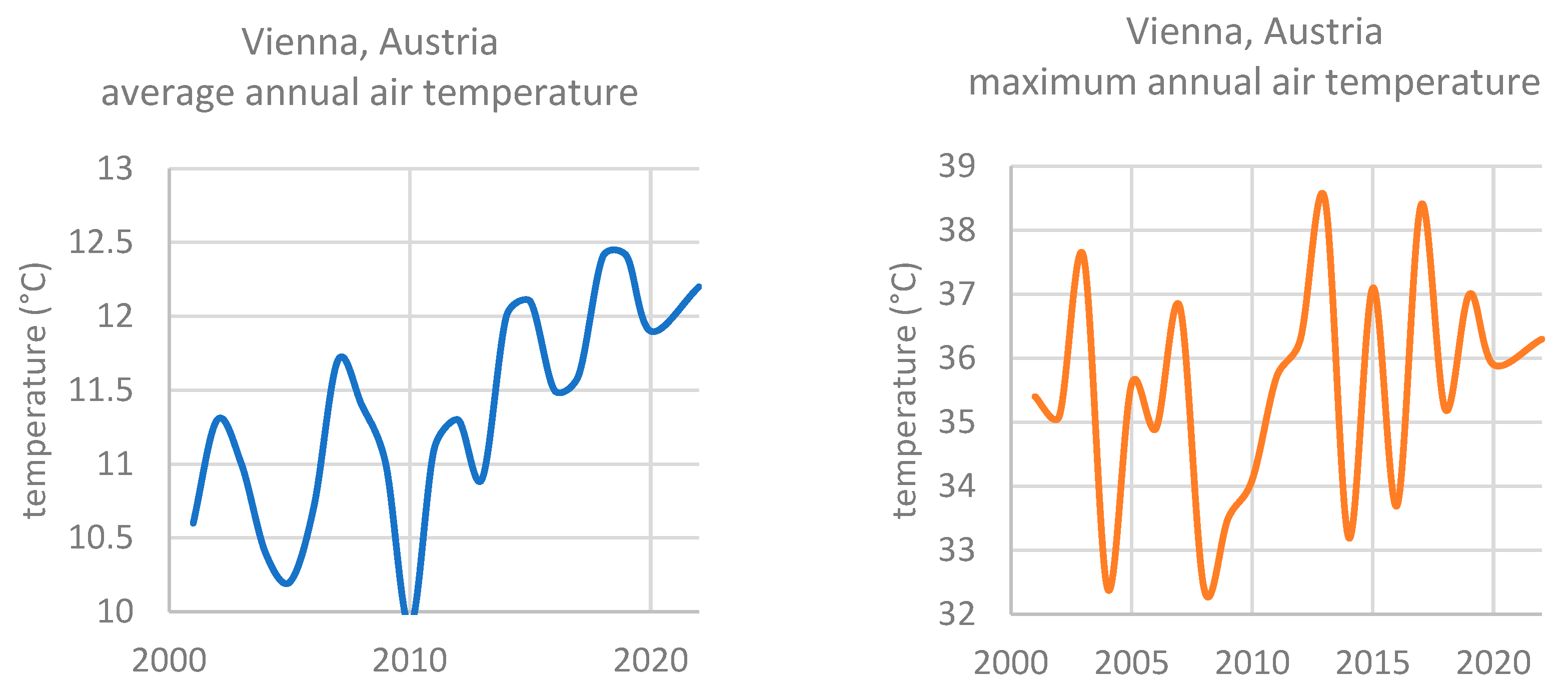
Large areas of natural vegetation are devoured by unrelenting urbanization, which replaces them with sealed surfaces and building structures with high heat storage mass and low-albedo surfaces such as asphalt concrete. The urban heat island (UHI) effect is a phenomenon caused by the thermal properties of the built environment and the absence of evapotranspiration in urban regions [1]. Additionally, statistics show that the average temperature in the middle of Europe is on a steady rise, which also means that the temperature maxima are rising more and more in the summer (Figure 1) [2].

The notion of reintroducing nature into the urban environment offers itself as a remedy for this. It is important to deepen the relationship between nature and the city in order to develop a new sustainable urban lifestyle. Building and maintaining greening may be a crucial component of this shift in areas of the world where greening is a viable option [3,4].

Meanwhile, the greening of roofs and walls has arisen as one of the most inventive and quickly evolving fields in the worlds of ecology, horticulture, and construction because the exterior surfaces of buildings provide significant space for plants in cities. Vertical greening strategies have great potential to help reduce the UHI effect through evapotranspiration, evaporation, and shading because there are so many building walls available [5]. Potential retrofitting techniques for the envelope of existing (heritage) buildings are presented in [6]. Vertical greening also has the potential to be a very efficient tool to increase a building’s exterior thermal insulation in the winter and to provide a defense against overheating in the summer, both of which improve the total energy efficiency [7]. The results from the literature survey in [7] show that green roofs and facades can be viewed as key solutions to reduce building-related energy consumption and greenhouse gas emissions during the lifetime of a building.

However, prior research has mostly concentrated on wall-mounted greening systems, which are often hung in front of the facade with a rear ventilation gap and consist of structures with planters, such as troughs or modules [8,9]. The characteristics of different versions of such green wall systems are shown in [10]. Even though self-climbing plants, such as ivy, have been used in green buildings for ages, research on how they affect building physics is still rare, and there is a dearth of information on their real insulation effects.

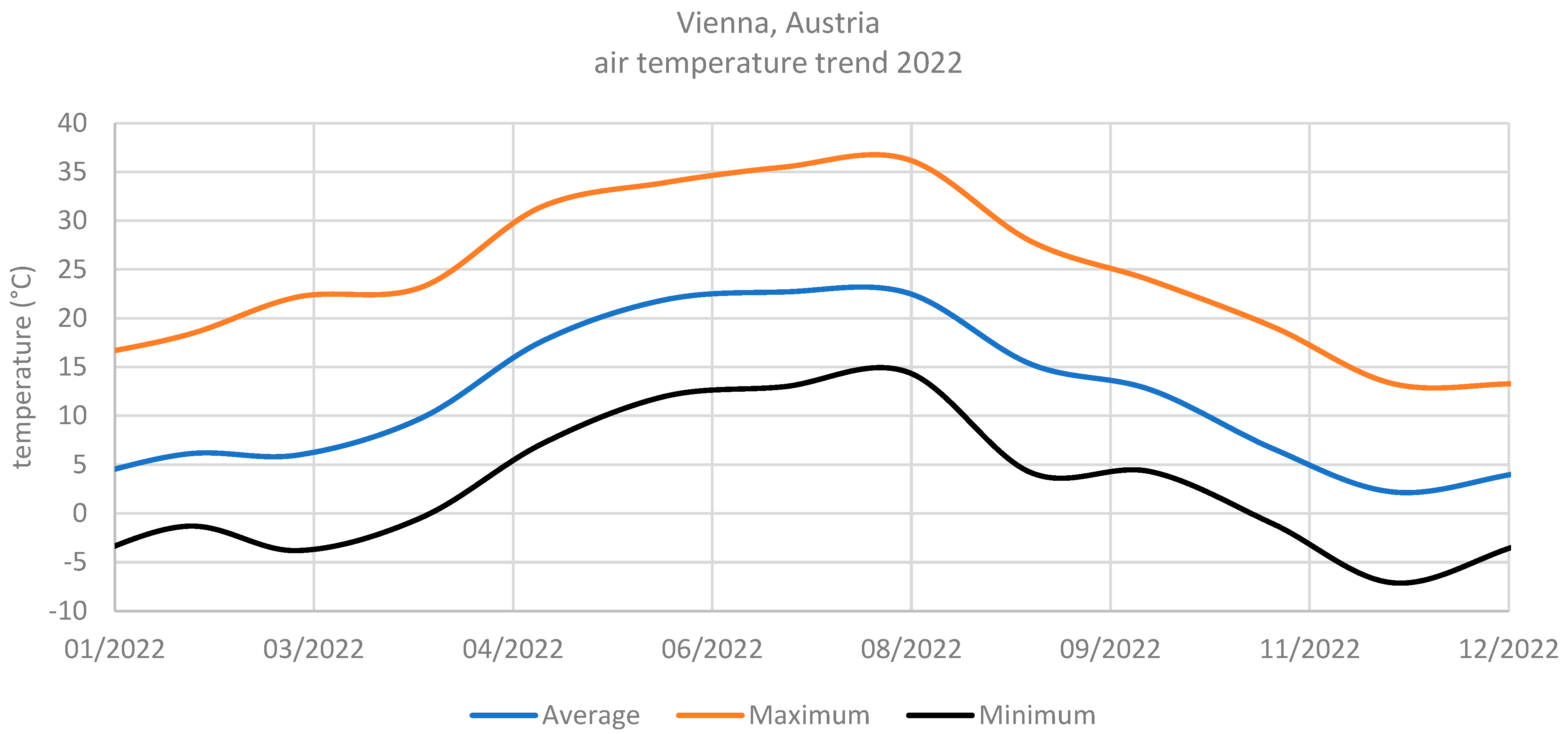
Research has been mostly concentrated on assessing the influence of various climbers on the summertime surface temperatures of buildings or building components [11,12,13,14] due to the absence of foliage in the winter months. Other research has only examined the influence of ivy on the microclimate [15], the influence of ivy on the surface temperature during cold months [16], and the impact of ivy on the moisture of masonry in contact with the ground [17]. In order to determine the impacts of ivy on the insulating characteristics of masonry, this study effort is focused on various effects in the winter (the heat flux density, exterior surface temperature, and heat transfer coefficient) and summertime (the exterior surface temperature). Evergreen ivy was chosen as the study subject so that measurements could be carried out for both the summer and winter months. As there are hardly any studies on the effects of ivy on the heat transfer coefficient in winter, this study tries to fill a research gap and identify possible positive effects in the winter months and aims to confirm the effects already found in other studies in the summer months. Vienna, Austria, is particularly suitable to study the effects of greening in different scenarios due to the relatively low temperatures in winter and high temperatures in summer, reaching, for example, from −5.3 °C in January up to 36.3 °C in August for the year 2022. Figure 2 shows the trend of the monthly average air temperature (the average, maximum, and minimum) throughout the year 2022 in Vienna, Austria, recorded by the “Zentralanstalt für Meteorologie und Geodynamik (ZAMG)” [18].

2. Materials and Methods

To determine the heat transfer coefficient of a facade by calculation (in accordance with ISO 13789 [19]), information about the components of the facade is needed. The thickness of each homogeneous layer and its thermal conductivity should be known. On many existing buildings, the heat transfer coefficient for individual sections of the facade cannot be reliably determined using this method. The thermal conductivity of the components may have changed over the decades due to aging processes or moisture uptake. Taking samples from the facade to measure the thermal conductivity is not practical. The heat transfer coefficient must, therefore, be determined by measurement (following ISO 9869 [20]). In the following, terms and definitions related to the in situ measurements are discussed. The relevant and investigated thermal properties of the facade are defined as follows:

• Surface temperature (T_s)

The surface temperature corresponds to the temperature measured directly on the surface on the inside (T_si) or outside (T_se) of the component. On the outside, it is significantly influenced by the external climate (temperature (T_e), solar radiation, wind, etc.), while on the inside, it depends mainly on the room air temperature (T_i), air movement, and room use. At the same time, the heat storage capacity and thermal conductivity of the building component influence the surface temperatures on both sides. In the case of the green facade, factors such as the slowing of air movement by the foliage, the dynamic shading coefficient [21], the absorptivity of the foliage, and evapotranspiration in summer are added as unknown influencing variables [12,22] that are not considered any further in the present experimental study.

• Heat flux density (q)

Heat flux density describes the heat transferred per defined area and time interval, thus corresponding to the thermal power per area, and it is given in watts per m². In the metrological recording with the aid of a heat flow measuring plate, the heat flow through the building component (masonry) is measured in the horizontal direction. The heat flow and its direction depend on the conditions prevailing in the interior or exterior space, since the heat energy always flows from an area with a higher temperature to an area with a lower temperature. Since the heat flow can change its direction, it can have both a positive sign (heat flowing out of the building) and a negative sign (heat flowing into the building). For the evaluation, this means that when comparing different series of measurements, the prevailing surface or air temperatures must also be considered at the same time, since the heat flow alone does not allow any statement to be made about the insulation properties of a building component.

• Heat transfer coefficient (U)

The heat transfer coefficient (HTC or U) is a measure of heat transfer through a building component. It is defined by equation 1, where q is the heat flux density (q), and T_i − T_e is the difference between the air temperature inside (T_i) and outside (T_e). A distinction is made between steady-state and transient heat transfer coefficients. The transient heat transfer coefficient is determined under transient boundary conditions, which makes the addition of other physical parameters necessary for the calculation. In the course of the present project, only the steady-state heat transfer coefficient was calculated, since this is decisive for the integration into the energy performance certificate (Energy Performance of Buildings Directive, 2010/31/EU [23]).

U = q/(T_i − T_e) = 1/R_T

(1)

Table 1. Measured values and corresponding sensors in use.

Parameter		Unit	Equipment	Accuracy
Heat flow	q	(W/m²)	Phymeas® (Cottbus, Germany), Heat flow measuring plate	±5%
Surface temperature, interior	Tsi	(°C)	RS PRO (Frankfurt am Main, Germany) PT1000 temperature probe	CLASS 5
Surface temperature, exterior	Tse
Air temperature, interior	Ti		TandD (Matsumoto, Japan), RTR 507B	±0.3 °C
Air temperature, exterior	Te

shows an overview of the measured values, the corresponding sensors in use, and their accuracy according to the data sheets.

In order to determine the effects of ivy on masonry walls, the following criteria were established for the selection of two buildings to be studied based on [22]:

• A thick leaf layer covering the outer wall;
• A relatively steady thermal load;
• No shading other than the ivy.

Consequently, two buildings in Vienna, Austria, were selected as objects of the study:

• Kopalgasse 7

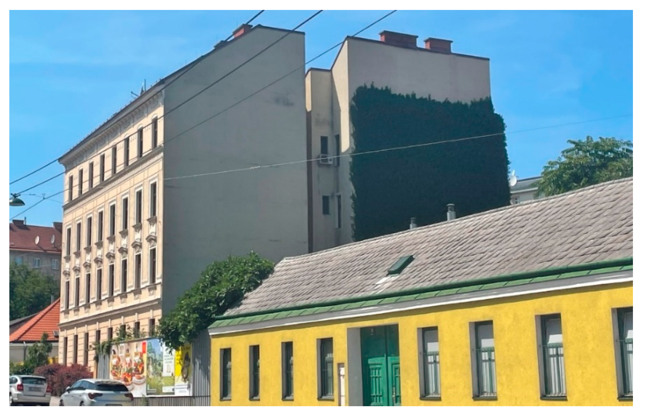
The property at Kopalgasse 7, in Vienna’s 11th district, is a residential building that was constructed around 1911 and has been repeatedly renewed and renovated over the course of its life cycle. A significant renovation or expansion of the exterior envelope, which is a masonry wall with a 40 cm thickness and 2 cm plaster on the inside, took place in 1987–1988. The building was insulated with 5 cm of EPS (expanded polystyrene) on the sides not facing the street, and in the course of the clean-up work after the thermal renovation, self-climbing facade greening was implemented on the facade facing east-northeast in the form of two ivy plants. According to the owners, conventional garden soil was used for this purpose, and the plants were not additionally watered or fertilized. The wall was fully overgrown after about 7 years and was regularly cut back from that point on to prevent overgrowth on the roof surfaces or other walls, reduce weight, and remove shoots and branches that could pose a danger to people nearby in windy conditions. This has resulted in dense and relatively uniform growth about 2 feet below the eaves. Figure 3 shows a photograph of the facade in the summer of 2021 from across the street.

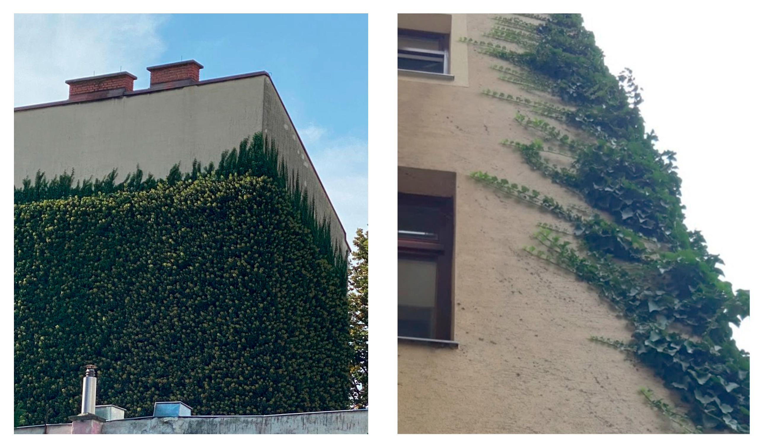
Over the course of the measurement period, the thickness of the vegetation layer over the entire area has been relatively uniform. At the beginning of the measurements, it was approximately 40 cm, and at the end, it was 50 cm. Any growth during the measurement period could be perceived mainly at the edges of the greenery (Figure 4). Pruning of the greenery usually takes place every 3 years.

2.

Muthgasse 109

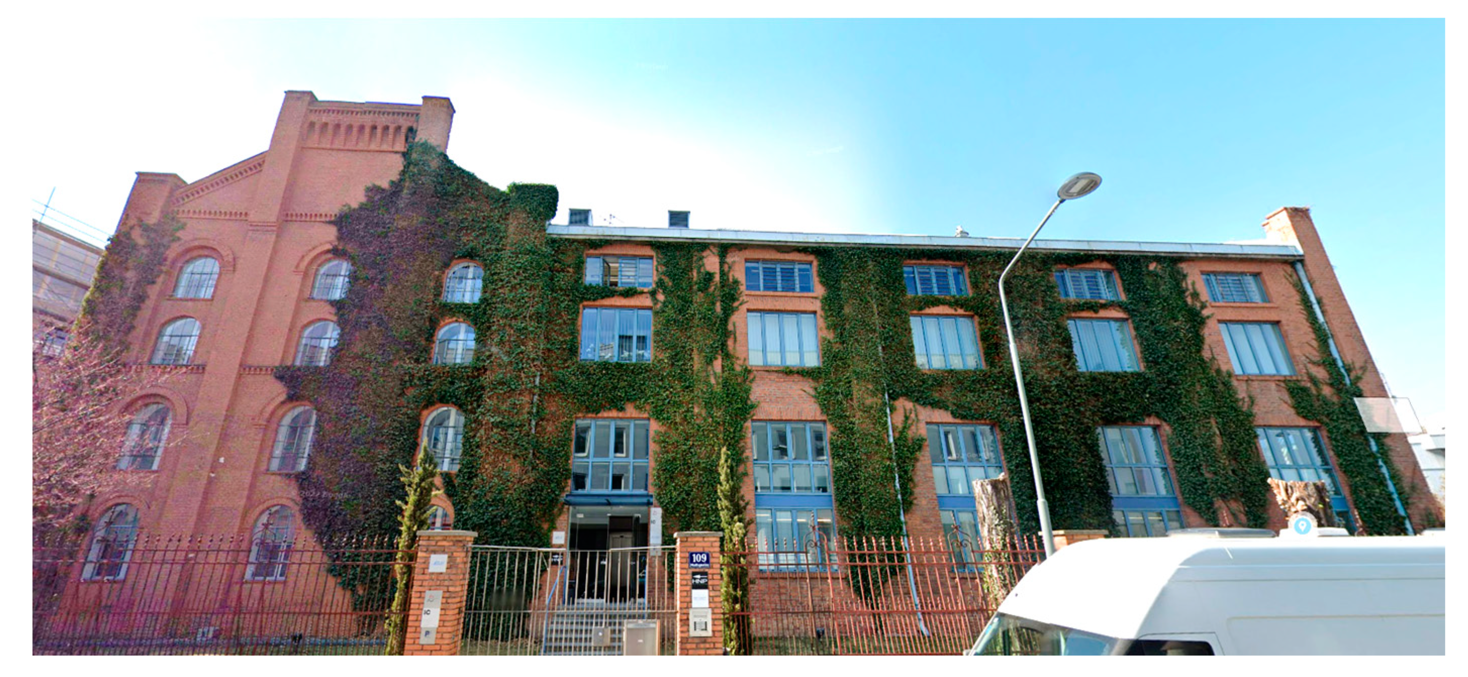
The property at Muthgasse 109 in Vienna’s 19th district is a former power plant that was built around 1897. A revitalization of the building took place in 1988. Thereby, the outer shell of the building, which is a masonry wall with a thickness of 60 cm, was not thermally renovated, and only the core was adapted to the new usage scenario. Sometime after the revitalization, a self-climbing facade greening was implemented on the east-facing and street-side facade in the form of 7 ivy plants (1995). According to the owners, conventional garden soil was used for this purpose, and the plants were not additionally watered or fertilized. The part of the building facing the street was almost completely overgrown after about 10 years (see Figure 5) and was cut back once a year from that point on to prevent overgrowth on the roof surface or other walls.

During the project period, pruning took place in March 2022. Thus, the thickness of the greening layer before the pruning was about 30–40 cm, and afterward, it was about 20–30 cm. Compared to the greening in the Kopalgasse, the vegetation was less dense and rather uneven when viewed over the entire facade. Thus, the results obtained also provide indications of the extent to which the differences in growth influence the effect of greening.

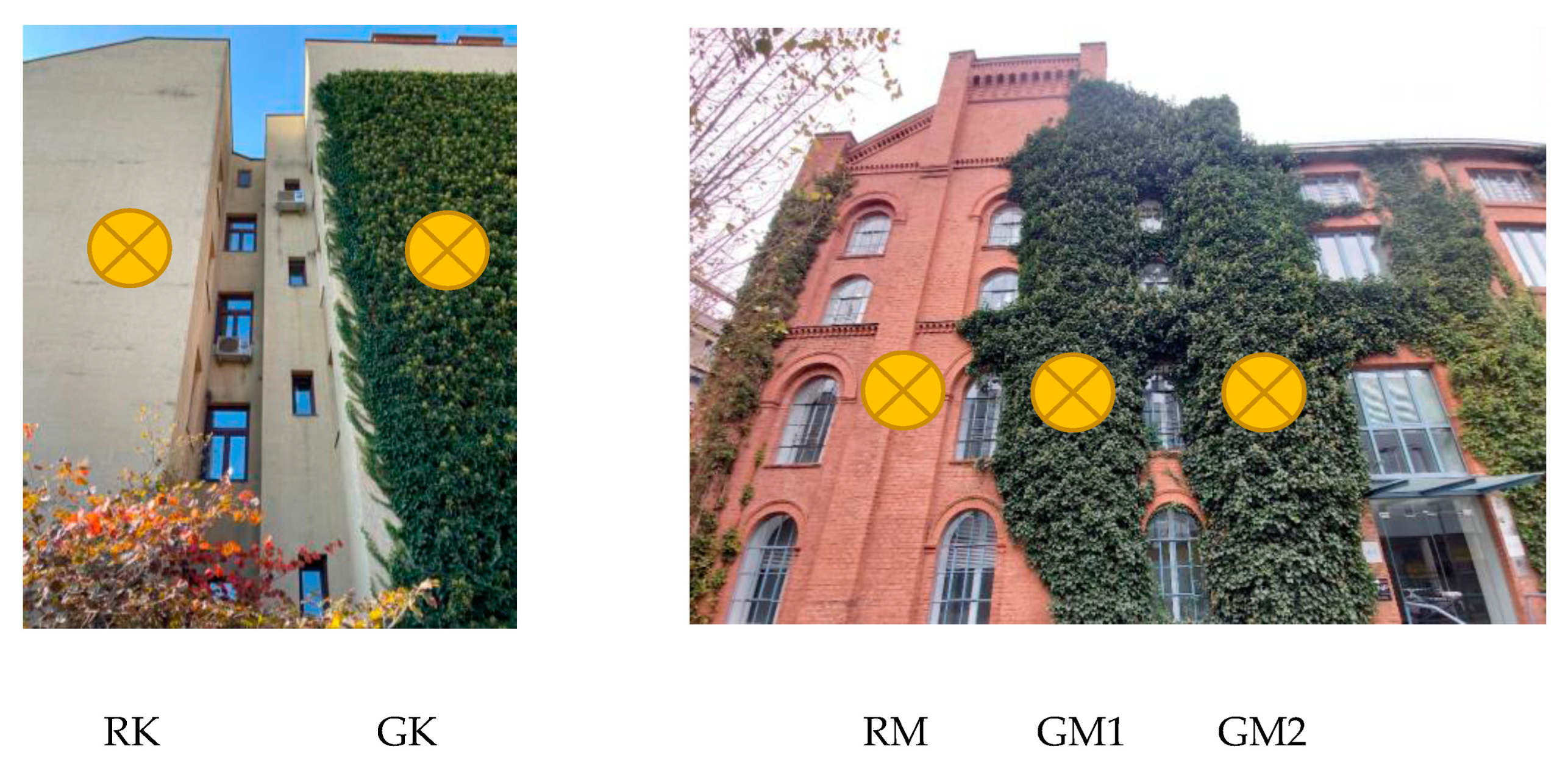
Figure 6 shows the chosen sensor positions for both buildings. In the following, the positions for the building in Kopalgasse are called RK (reference) and GK (greened), and the positions for the building in Muthgasse are called RM, GM1, and GM2. The sensors at position RK and GK were installed in November 2021, and the sensors at position RM and GM1 in December 2021. The sensors at position GM2 were installed later in March 2022 to validate the results obtained from GM1 due to the relatively high fluctuation in leaf density across the ivy plant.

3. Results

Due to the complexity of the data and regulations from standard ISO 9869 [20], various filter criteria had to be defined and applied for the evaluation. For filtering and calculating the results, the data, which were collected in time intervals of 3 to 5 min, were ultimately summarized in 10 min averages. For the presentation of the data in the xy diagrams, 1 h averages were then calculated from the 10 min averages. For the analysis of the winter and summer, the criteria that were chosen are explained in the following.

3.1. Winter

The measurement data collected in winter were used for the metrological determination of the heat transfer coefficient due to the high and relatively constant temperature differences between the interior and exterior. To be able to determine the steady-state heat transfer coefficient, the following filter criteria were applied:

• The temperature difference between the interior and exterior surfaces must be at least 15 Kelvin: T_si − T_se > 15 K;
• The exterior surface temperature must not have changed by more than 2 °C in the last 24 h.

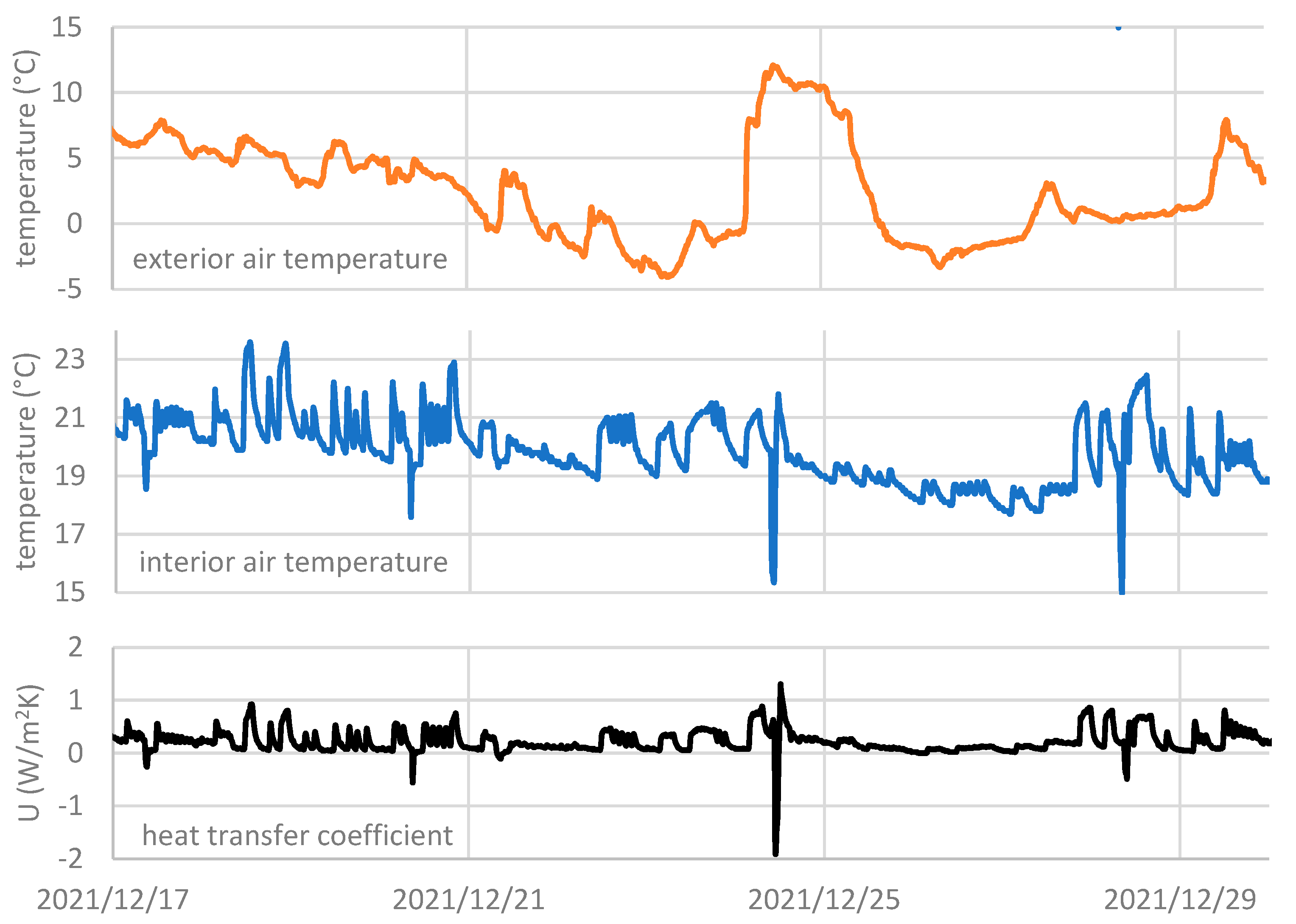
Fluctuations of the interior room temperature caused by the occupants have a significant influence on the measurement of the heat flux density (q) and, subsequently, the heat transfer coefficient (U), which leads to a relatively high standard deviation and should be considered when interpreting the results. Figure 7 shows the heat transfer coefficient (U) in comparison to the exterior and interior temperature for an exemplary period in December 2021 at the Kopalgasse.

3.1.1. Heat Transfer Coefficient (U)

The filtered data were used to calculate the heat transfer coefficient for three consecutive winter months.

• Kopalgasse

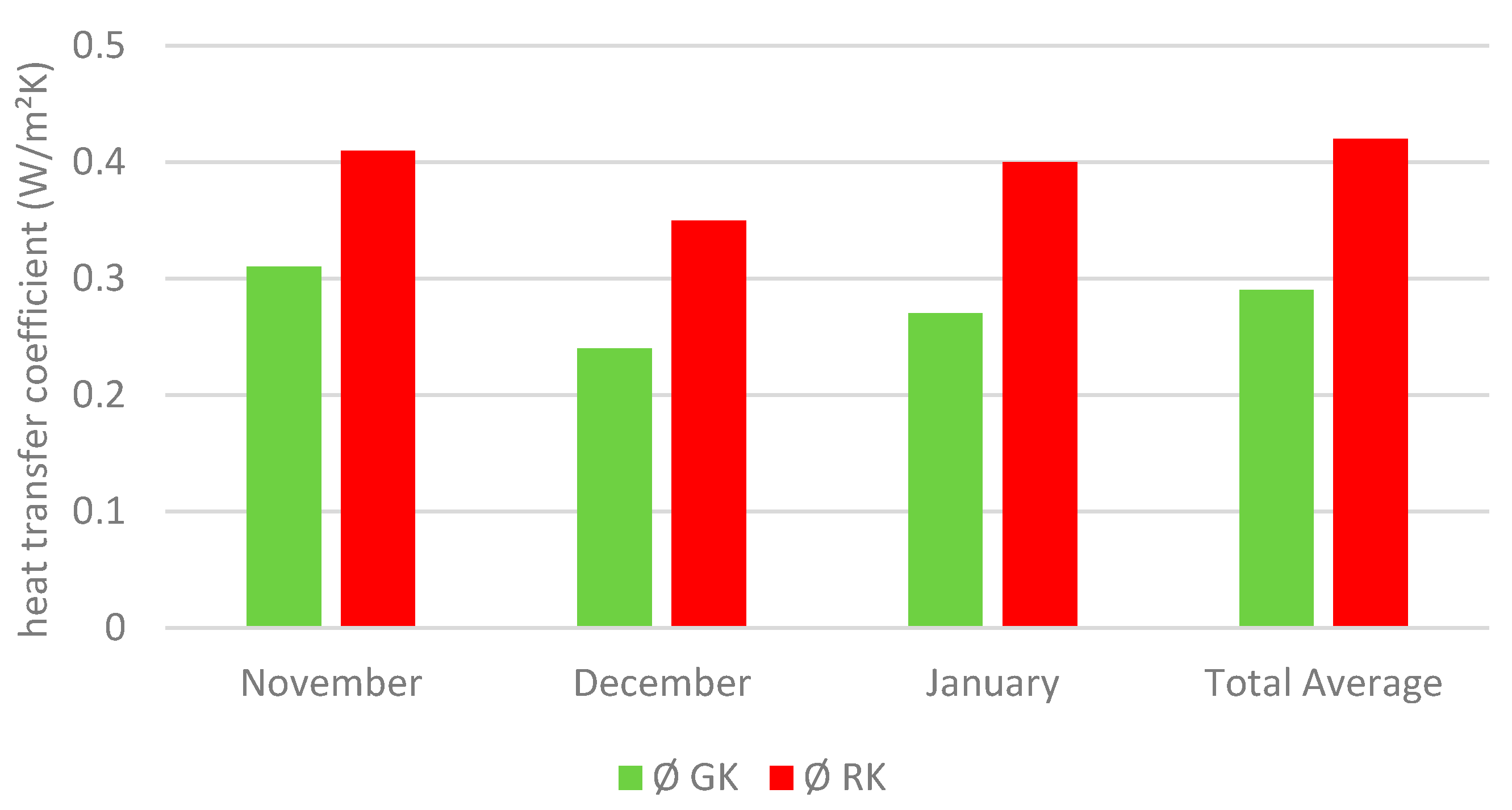
For Kopalgasse, the results are shown in

Table 2. Heat transfer coefficient, Kopalgasse, average during winter, filtered data.

	Filtered Data
	Ø U (W/m2K)
	GK	RK	Reduction in W/m2K	Reduction in %
November	0.31 ± 0.18	0.41 ± 0.12	0.10	26
December	0.24 ± 0.22	0.35 ± 0.08	0.11	32
January	0.27 ± 0.18	0.40 ± 0.13	0.13	32
Total Average	0.27 ± 0.03	0.39 ± 0.03	0.11 ± 0.01	30 ± 3

and Figure 8. Looking at the data obtained, a relatively clear picture of the effect of greening on the building’s walls emerges. On average, the ivy in Kopalgasse leads to a 30 ± 3% reduction in the heat transfer coefficient of the old masonry wall (old brick) insulated with 5 cm of EPS. The small standard deviation of 3% shows that the effect was relatively constant and reproducible when looking at and comparing individual months. This suggests that the benefits of greening persist throughout the winter.

• Muthgasse

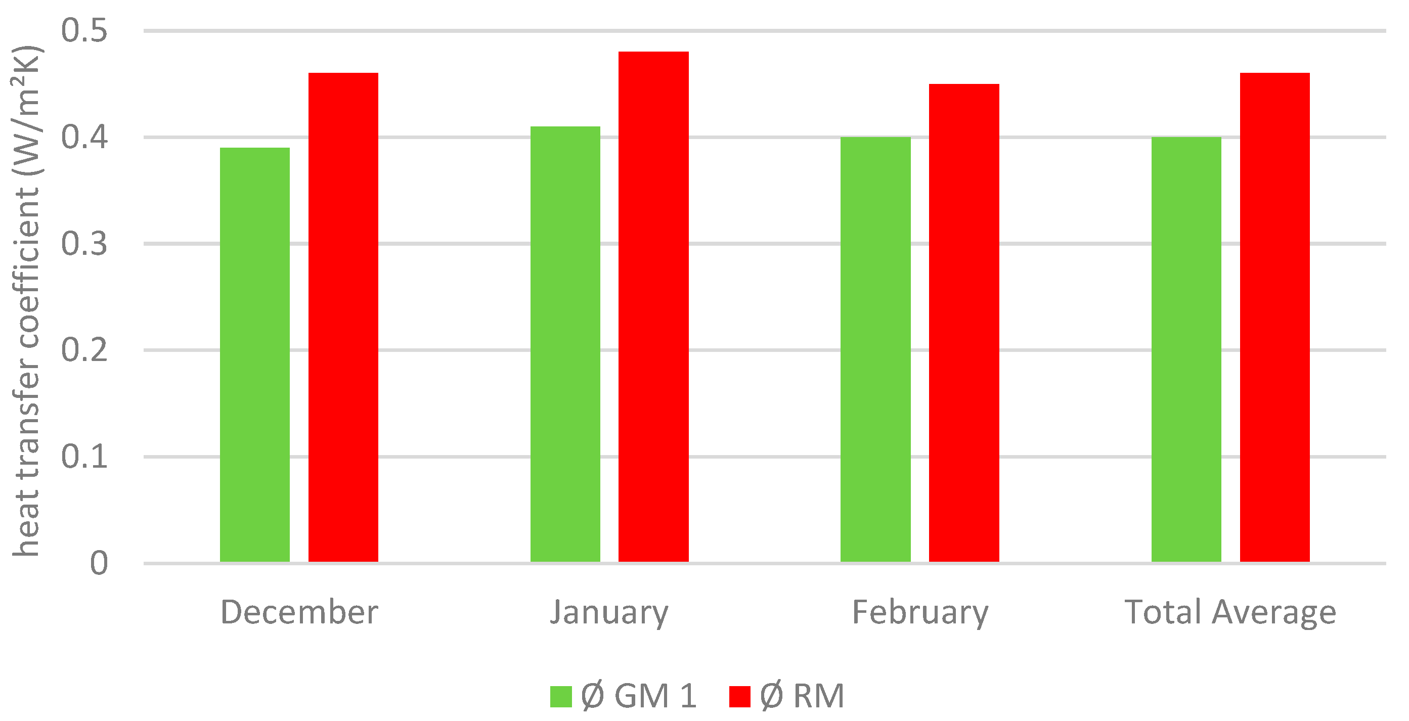
For Muthgasse, the results are presented in

Table 3. Heat transfer coefficient, Muthgasse, average during winter, filtered data.

	Filtered Data
	Ø U (W/m2K)
	GM1	RM	Reduction in W/m2K	Reduction in %
December	0.39 ± 0.15	0.46 ± 0.18	0.07	15
January	0.41 ± 0.11	0.48 ± 0.12	0.07	15
February	0.40 ± 0.07	0.45 ± 0.08	0.05	11
Total Average	0.40 ± 0.01	0.46 ± 0.01	0.06 ± 0.01	14 ± 2

and

Table 4. Heat transfer coefficient, Muthgasse, average during winter, filtered data.

	Filtered Data
	Temperature Difference and Heat Flux Density
	Ø Tsi − Tse (°C)		Ø Ti − Te (°C)		Ø Heat Flux Density (W/m2)
	Green	Reference	Green	Reference	Green	Reference
December	16.4 ± 0.9	18.1 ± 1.3	21.0 ± 1.6	20.9 ± 1.6	6.7 ± 0.6	7.9 ± 0.5
January	16.3 ± 0.8	18.0 ± 1.3	20.5 ± 1.5	20.4 ± 1.5	6.8 ± 0.9	8.2 ± 1.0
February	20.1 ± 4.3	21.0 ± 3.3	20.6 ± 2.6	20.7 ± 2.6	8.2 ± 1.1	9.3 ± 1.2
Total Average	17.6 ± 2.2	19.0 ± 1.7	20.7 ± 0.3	20.7 ± 0.3	7.2 ± 0.8	8.5 ± 0.7

and Figure 9. Compared to Kopalgasse, the effect of greening on the heat transfer coefficient is significantly lower. With an average reduction of 14%, the effect is about half of the effect in Kopalgasse. The relatively low standard deviation of 2% shows that the effect is reproducible and has therefore persisted over the months investigated.

3.1.2. Surface temperature (T_si, T_se)

For the evaluation of the surface temperatures, the mean values and standard deviation, as well as the maximum and minimum of the unfiltered data, were calculated for the winter months.

• Kopalgasse

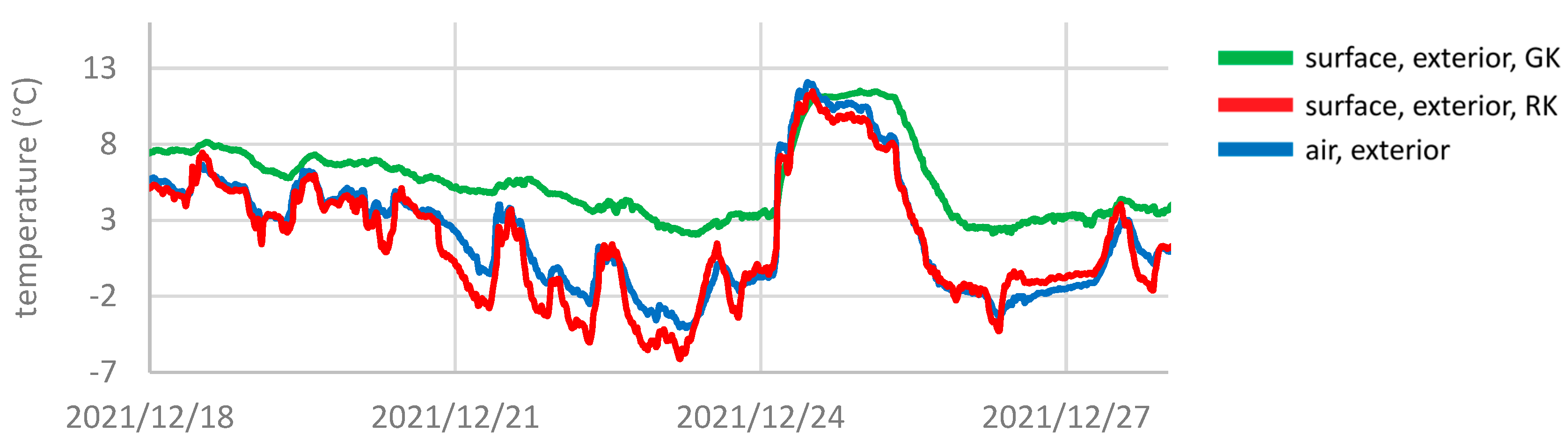
Based on the results presented in

Table 5. Surface temperature, exterior, Kopalgasse, average values of the winter months, unfiltered data.

	Unfiltered Data
	Surface Temperature, Exterior (°C)
	GK		RK		GK	RK	Difference in °C	Difference in %
	Min.	Max.	Min.	Max.	Average	Average
November	4.7	12.6	−2.4	14.2	7.7 ± 2.1	4.2 ± 3.2	3.5	45
December	2.1	14.3	−6.1	15.2	6.7 ± 2.6	3.5 ± 3.9	3.2	48
January	1.2	14.3	−6.3	15.8	6.2 ± 2.9	3.7 ± 3.9	2.5	40
Average	2.7 ± 1.8	13.7 ± 1.0	−4.9 ± 2.2	15.1 ± 0.8	6.9 ± 0.8	3.8 ± 0.4	3.1 ± 0.5	44 ± 4

, it can be seen that the greening increased the temperature on the outside of the facade by an average of about 3 °C or 44% over the months considered. Based on the standard deviation of the individual months, it can be seen that there was less temperature fluctuation overall for the greened component. Figure 10 shows an example of the temperature variation in winter. The surface temperature of the reference (not green) follows the outside air temperature for the most part and even drops below the outside air temperature during particularly low temperatures and certain weather conditions (wind). The greened wall section, on the other hand, is protected by the plant and cools down less, accordingly. In the period shown in Figure 10 for example, the temperature did not fall below approx. 3 °C on position GK, while at the same time, the temperature of RK was as low as approx. −5 °C. Based on the maximum and minimum, it can be seen that the minimum temperatures of the reference were lower by 7.1 °C (cf. 4.7 and −2.4) in November, 8.2 °C (cf. 2.1 and −6.1) in December, and 7.5 °C (cf. 1.2 and −6.3) in January. The observed maximum temperatures at the reference give clear indications of the effects of solar radiation. Due to the shading of the plants, the maximum temperature at position GK thus, on average, was 1.4 °C lower than at the reference.

• Muthgasse

Table 6. Surface temperature, exterior, Muthgasse, average values of the winter months, unfiltered data.

	Unfiltered Data
	Surface Temperature, Exterior (°C)
	GM1		RM		GM1	RM
	Min.	Max.	Min.	Max.	Average	Average	Difference in °C	Difference in %
December	0.8	12.2	−2.0	11.2	5.0 ± 2.9	3.9 ± 3.6	1.1	21
January	−0.3	13.4	−3.6	13.3	5.4 ± 2.9	4.2 ± 3.3	1.2	22
February	4.2	14.9	0.9	14.9	8.6 ± 2.3	7.3 ± 2.8	1.3	15
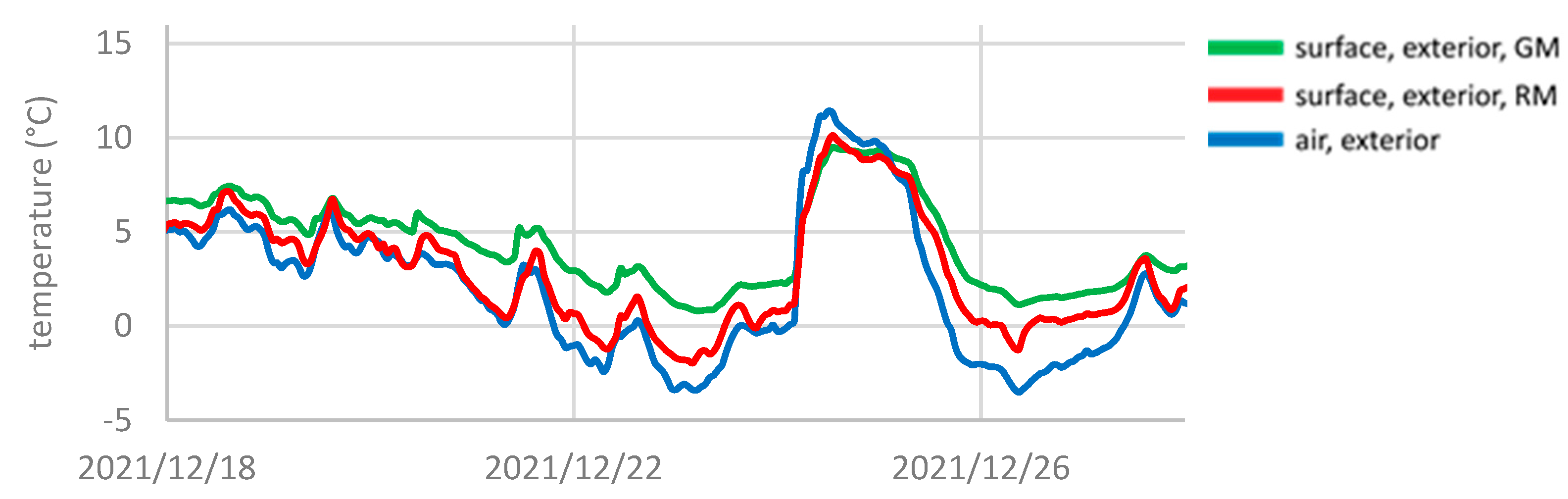
Average	1.6 ± 2.3	13.5 ± 1.4	−1.6 ± 2.3	13.1 ± 1.9	6.3 ± 2.0	5.1 ± 1.9	1.2 ± 0.1	19 ± 4

shows the calculated values for the relevant winter months at Muthgasse. On average, the temperature at the greened measuring point was 1.2 °C higher than at the reference, which corresponds to an overall average difference of approx. 19%. Figure 11 shows an example of a section of the recorded data in January 2022. During the period under consideration, the air temperature outside, and thus also the surface temperatures, changed relatively strongly. Basically, the surface temperature at GM1 was consistently higher than at the reference (RM). As the air temperature increases, the difference between the greening and reference decreases. This can also be seen in the data in Table 6. For example, the difference between the maximum temperatures reached by the greening and reference in December was only 1 °C (cf. 12.2 and 11.2), in January, even only 0.1 °C (cf. 13.4 and 13.3), and in February, 0 °C (cf. 14.9 and 14.9). The minimum temperatures, on the other hand, differ significantly. In December, the reached minimum temperatures differed by 2.8 °C (cf. 0.8 and −2.0), in January by 3.3 °C (cf. −0.3 and −3.6), and in February by 3.3 °C (cf. 4.2 and 0.9).

3.2. Summer

The data collected in the summer was used to evaluate the impact of greening on the surface temperatures only due to the high fluctuations of the heat flux density, which also resulted in a reversal of the sign. For this purpose, in order to be able to present the effect as clearly as possible, the measured data were analyzed for the presence of heat waves. The following filter criteria were applied. The air temperature (outside) must have been at least 30 °C for three consecutive days.

Surface Temperature

To evaluate the effect, especially during heat waves, the data were filtered based on the definition of a heat wave according to the “Zentralanstalt für Meteorologie und Geodynamik (ZAMG)” in accordance with Kysely [2]. Following this, a heat wave is present when the exterior air temperature has been at least 30 °C for three consecutive days. To show the influence of the filtering on the calculated averages, the unfiltered data are presented as well.

• Kopalgasse

Table 7. Surface temperature exterior, Kopalgasse, average values of the summer months, unfiltered data.

	Unfiltered Data
	Surface Temperature, Exterior (°C)
	GK		RK		GK	RK	Difference
	Min.	Max.	Min.	Max.	Average		Average	Max.
June	18.3	30.4	15.8	40.6	24.2 ± 2.3	26.2 ± 5.3	2.0 ± 4.8	16.7
July	18.0	31.2	15.8	43.9	25.1 ± 2.8	26.5 ± 5.9	1.4 ± 4.9	17.3
August	19.5	31.3	17.1	41.1	24.7 ± 2.3	25.7 ± 5.2	1.0 ± 4.2	13.3
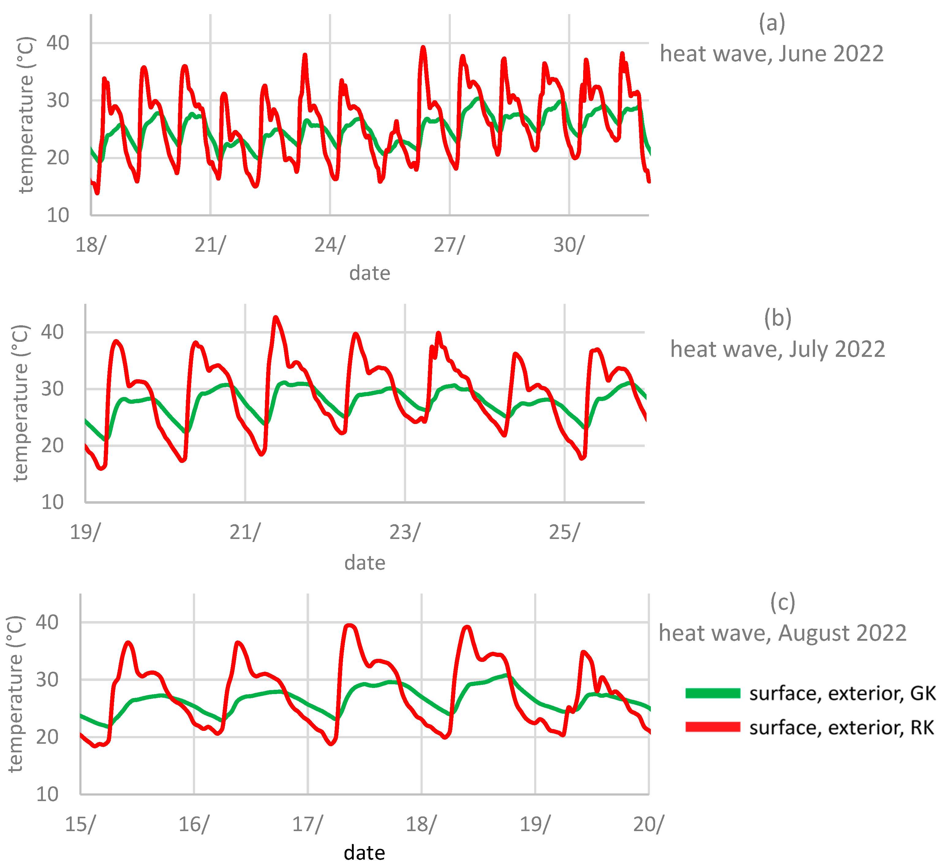
Total Average	18.6 ± 0.6	31.0 ± 0.4	16.2 ± 0.6	41.9 ± 1.5	24.7 ± 0.4	26.1 ± 0.3	1.5 ± 0.4	15.8 ± 1.8

shows the calculated mean and standard deviation of the exterior surface temperature of the unfiltered data, and

Table 8. Surface temperature exterior, Kopalgasse, average values of the summer months, filtered data.

	Filtered Data
	Surface Temperature, Exterior (°C)
	GK		RK		GK	RK	Difference
Heat Wave	Min.	Max.	Min.	Max.	Average		Average	Max.
June	19.5	30.4	16.0	39.8	25.5 ± 2.3	26.9 ± 5.6	1.4 ± 4.7	14.8
July	21.2	31.2	17.3	43.2	27.5 ± 2.3	28.8 ± 6.2	1.3 ± 5.0	14.3
August	21.9	30.8	18.3	41.0	26.0 ± 2.2	26.9 ± 5.6	0.9 ± 3.7	13.3
Total Average	20.9 ± 1.0	30.8 ± 0.3	17.2 ± 0.9	41.3 ± 1.4	26.3 ± 0.8	27.5 ± 0.9	1.2 ± 0.2	14.1 ± 0.6

shows the corresponding values for the evaluated heat waves during the summer months. As can be seen, the effect of the ivy layer was relatively variable over the summer. For example, the greened monitoring site was, on average, 1.4 and 1.3 °C cooler than the reference during the heat waves in June and July, respectively, and 0.9 °C cooler in August. The difference in August is likely primarily due to the overall lower temperatures in August. For example, the maximum temperature difference during the August heat wave was only 13.3 °C, whereas, during the June and July heat waves, it was 14.8 and 14.3 °C, respectively. On average, the difference in the unfiltered summer data has been 1.5 ± 0.4 °C, and the maximum difference has been 15.8 ± 1.8 °C.

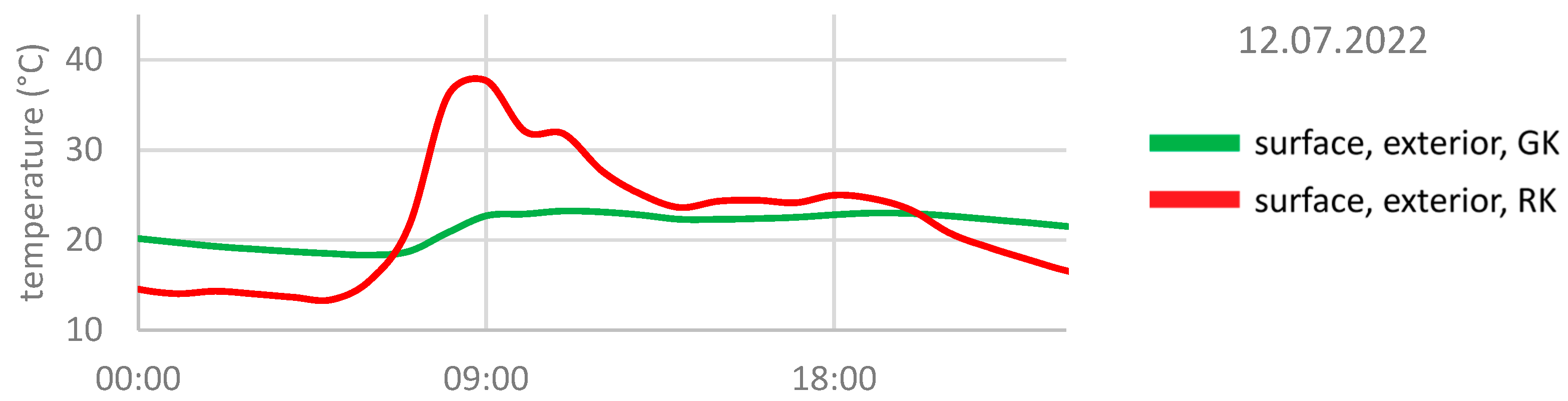
Figure 12a–c show the course of the surface temperatures during the individual heat waves. As can be clearly seen, the greening causes the facade to heat up less during the day and cool down less during the night. This results in less fluctuation in the temperatures overall. For example, during the heat wave in July, the maximum surface temperature was 43.2 °C for the reference and only 31.2 °C for the greening. During the same period, the minimum surface temperature was 17.3 for the reference and 21.2 °C for the surface under the vegetation. The highest difference between the reference and vegetation was measured on 12 July 2022, with 17.3 °C (also see Table 8). To take a closer look at the temperature curve on this day, it is shown in Figure 13. The maximum temperature difference is reached at about 8:00. The temperature peak, occurring at approx. 9:00 o’clock for the reference, is typical for the summer days considered and can be found for almost all the days. Due to the exposure and orientation of the facade, it can be attributed to direct exposure to solar radiation. The absence of these temperature peaks in the greening, thus, mainly shows the effect of shading by the climbing plants.

• Muthgasse

Table 9. Surface temperature exterior, Muthgasse, average values of the summer months, unfiltered data.

	Unfiltered Data
	Surface Temperature, Exterior (°C)
	GM1		GM2		RM		GM1	GM2	RM
	Min.	Max.	Min.	Max.	Min.	Max.	Average	Average	Average
June	15.6	33.4	14.5	32.0	15.6	44.1	24.4 ± 3.7	23.9 ± 3.5	26.2 ± 6.1
July	18.1	33.6	18.5	32.3	16.6	43.8	25.5 ± 3.7	25.2 ± 3.1	26.6 ± 6.4
August	18.5	33.7	18.8	31.5	17.1	44.8	25.2 ± 3.2	24.9 ± 2.6	26.0 ± 5.7
Average	17.4 ± 1.3	33.6 ± 0.1	17.3 ± 2.0	31.9 ± 0.3	16.0 ± 0.6	44.2 ± 0.4	25.0 ± 0.5	24.7 ± 0.6	26.3 ± 0.2

shows the calculated mean or standard deviation of the exterior surface temperature of the unfiltered data, and

Table 10. Surface temperature exterior, Muthgasse: average values of the summer months, filtered data.

	Filtered Data
	Surface Temperature, Exterior (°C)
	GM1		GM2		RM		GM1	GM2	RM
Heat Wave	Min.	Max.	Min.	Max.	Min.	Max.	Average	Average	Average
June	16.7	33.4	16.7	32.0	16.5	44.1	26.4 ± 3.4	26.0 ± 3.1	28.2 ± 6.0
July	21.7	33.6	22.0	32.3	19.3	43.8	28.7 ± 3.2	28.2 ± 2.6	30.3 ± 6.3
August	22.5	33.3	22.7	31.1	20.7	44.1	27.3 ± 2.9	26.7 ± 2.2	28.4 ± 5.7
Average	20.3 ± 2.6	33.4 ± 0.1	20.5 ± 2.7	31.8 ± 0.5	18.8 ± 1.7	44.0 ± 0.1	27.5 ± 0.9	27.0 ± 0.9	29.0 ± 0.9

shows the corresponding values for the evaluated heat waves in the summer months. The resulting differences between greening 1 and greening 2 and the reference are shown in

Table 11. Surface temperature, exterior, Muthgasse: difference between summer months, unfiltered data.

	Unfiltered Data
	Surface Temperature, Exterior (°C)
	GM1		GM2
	Difference		Difference
	Average	Maximum	Average	Maximum
June	1.8 ± 3.4	11.8	2.3 ± 3.9	13.7
July	1.1 ± 3.3	12.0	1.4 ± 3.8	13.9
August	0.8 ± 2.9	11.3	1.1 ± 3.5	13.6
Average	1.2 ± 0.4	11.7 ± 0.3	1.6 ± 0.5	13.7 ± 0.1

and

Table 12. Surface temperature, exterior, Muthgasse: difference between summer months, filtered data.

	Filtered Data
	Surface Temperature, Exterior (°C)
	GM1		GM2
	Difference		Difference
	Average	Maximum	Average	Maximum
June	1.8 ± 3.4	11.8	2.2 ± 3.9	13.7
July	1.5 ± 3.6	12.0	2.1 ± 4.2	13.9
August	0.9 ± 3.1	11.3	1.4 ± 3.7	13.6
Average	1.4 ± 0.4	11.7 ± 0.3	1.9 ± 0.4	13.7 ± 0.1

.

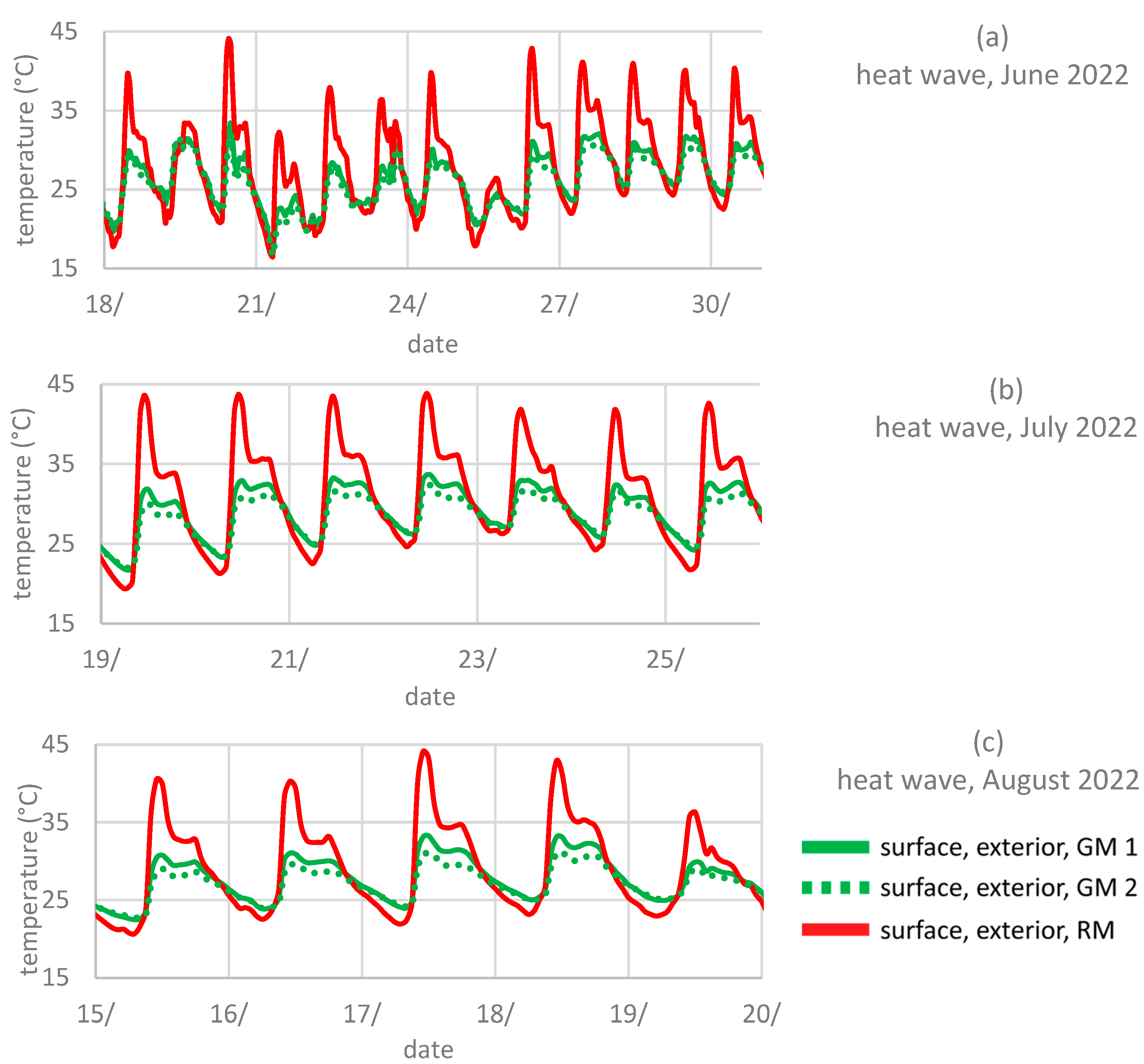
Similar to the data of Kopalgasse, the effect of greening fluctuated between the individual summer months. During the heat waves, the average difference between the greened measuring point and the reference was 1.8 °C for “GM1” in June and 1.1 °C and 0.8 °C in July and August, respectively, and 2.3 °C for “GM2” in June and 1.4 °C and 1.1 °C in July and August, respectively. The impact at the “greening 2” measurement site was thus stronger, which can be attributed to the denser growth at the measurement site and confirms the assumption that there is still potential at the Muthgasse site with regard to the impact of greening. The calculated maximum values can also be taken from Table 11 and Table 12.

The course of the surface temperature outside during the examined heat waves is shown in Figure 14. As can be seen, the course is very similar to that at the Kopalgasse site, whereby the stronger effect of the second measuring point (greening 2) can also be seen.

4. Discussion

On the basis of the investigations carried out, a positive effect of the greening at both locations could be clearly established, irrespective of the winter and summer seasons. Due to the reduction of the heat transfer coefficient, the heating demand in winter is reduced, and in summer, the surface temperature in the interior can be lowered. At the same time, the greening prevents large temperature maxima and temperature fluctuations on the external surface of the building, thus reducing the load on the building materials due to temperature changes. However, since both facades were not facing south, the results for south-facing facades could differ from the found results since exposure to sun and solar radiation is greater. Greening also partially reduces the cooling of the facade at night and thus leads to higher surface temperatures during nights in the summer. Since the heat flux density depends on the temperature difference between the inside and outside, greening has no significant effect on it during the transition period between seasons since the temperature difference is low in comparison to the summer and winter months. A comparable study examining the surface temperature on a greened east-facing exterior facade and a non-greened reference found an average reduction in the surface temperature of 2.2 °C (max. 13.9 °C) due to ivy [5].

Table 13. Results of the exterior surface temperature in comparison with other investigations.

		Kopalgasse (Table 7)	Muthgasse (Table 9)	Hoelscher et al. [13]
Reduction of exterior surface-temperature (Tse)	Average	1.5	1.4 (1.9) 1	2.2
	Maximum	15.8	11.7 (13.7) 1	13.9

¹ Values in parentheses represent the data for the measuring point GM2.

shows the results in comparison with the data from the Kopalgasse and Muthgasse sites, with the values in parentheses representing the data for the measuring point GM2.

When comparing the data for the heat transfer coefficients of the two buildings, it can be seen that the effect is significantly stronger on the Kopalgasse property. This is due to differences in the albedo and absorptivity of the facades (brick vs. plaster) and due to the different nature of the climbing plants, as the “greening layer” in the Kopalgasse appears not only more uniform and thicker but, above all, also denser. Thus, to reproduce the effect of the climbing plants from building to building, the nature of the plants must be similar (age, size, thickness, density, leaf area, etc.). In order to be able to use climbing plants in a targeted manner, parameters and guideline values must be defined; for example, planning tools to compare climbing plants in a simple way and to estimate their effects. Thus, there is a need for further research, especially concerning the definition and description of climbing plants and the creation of objective characteristic values for planning purposes. At the same time, these values can serve as a useful basis for the integration of climbing plants in simulations and other calculation methods (energy performance certificates).

5. Conclusions

The results of this study suggest that ivy greening can have a significant impact on the thermal performance of masonry walls. During the winter, the heat transfer through greened walls was found to be up to 30% lower compared to non-greened walls. This indicates that ivy greening can help reduce energy consumption for heating and thus improve the energy efficiency of buildings in all regions of the world where ivy greening can grow and prosper.

In addition, the surface temperature under the ivy was found to be significantly higher than on the bare wall during winter, which can help reduce the risk of moisture accumulation and mold growth. However, during the summer, the surface temperature under the ivy was lower than on the bare wall during the daytime, which may help reduce cooling energy consumption.

The results of this study are consistent with previous research in the field. It is important to note that the surface and air temperatures on the inside did not show clear results, which requires further investigation, and future studies must consider examining the exact density, size, leaf area index, and shading coefficient of the investigated plants on site. Otherwise, a comparison of different studies will be nearly impossible, and the results will not lead to generalizable statements.

Overall, this study provides valuable insights into the potential benefits of ivy greening on thermal performance. Since only a blank and a plastered masonry wall were examined, the research is representative of European “Gründerzeit” houses. These findings could be used to enhance, improve, and amend the design and construction of energy-efficient buildings in the future.

However, studies have shown that when utilizing ivy as an energy saver, older brickwork that is not plastered might be damaged by planting if ivy penetrates and expands in faults such as cracks [24,25]. At the same time, the planting shields the facade from rain, extreme temperature swings, and radiation [24]. As a result, potential negative consequences must be assessed individually based on the construction project.

References

- Mohajerani, A.; Bakaric, J.; Jeffrey-Bailey, T. The urban heat island effect, its causes, and mitigation, with reference to the thermal properties of asphalt concrete. J. Environ. Manag. 2017, 197, 522–538. [Google Scholar] [CrossRef] [PubMed]
- Zentralanstalt für Meteorologie und Geodynamik Zamg. Hitzewellen: 2015 Eines der Extremsten Jahre der Messgeschichte. Available online: https://www.zamg.ac.at/cms/de/klima/news/hitzewellen-2015-eines-der-extremsten-jahre-der-messgeschichte (accessed on 14 March 2023).
- Balany, F.; Ng, A.W.; Muttil, N.; Muthukumaran, S.; Wong, M.S. Green Infrastructure as an Urban Heat Island Mitigation Strategy—A Review. Water 2020, 12, 3577. [Google Scholar] [CrossRef]
- Marando, F.; Heris, M.P.; Zulian, G.; Udías, A.; Mentaschi, L.; Chrysoulakis, N.; Parastatidis, D.; Maes, J. Urban heat island mitigation by green infrastructure in European Functional Urban Areas. Sustain. Cities Soc. 2022, 77, 103564. [Google Scholar] [CrossRef]
- Price, A.; Jones, E.C.; Jefferson, F. Vertical Greenery Systems as a Strategy in Urban Heat Island Mitigation. Water Air Soil Pollut. 2015, 226, 247. [Google Scholar] [CrossRef]
- Santi, G.; Bertolazzi, A.; Leporelli, E.; Turrini, U.; Croatto, G. Green Systems Integrated to the Building Envelope: Strategies and Technical Solution for the Italian Case. Sustainability 2020, 12, 4615. [Google Scholar] [CrossRef]
- Besir, A.B.; Cuce, E. Green roofs and facades: A comprehensive review. Renew. Sustain. Energy Rev. 2018, 82, 915–939. [Google Scholar] [CrossRef]
- Tudiwer, D.; Teichmann, F.; Korjenic, A. Thermal bridges of living wall systems. Energy Build. 2019, 205, 109522. [Google Scholar] [CrossRef]
- Tudiwer, D.; Korjenic, A. The effect of living wall systems on the thermal resistance of the façade. Energy Build. 2017, 135, 10–19. [Google Scholar] [CrossRef]
- Manso, M.; Castro-Gomes, J. Green wall systems: A review of their characteristics. Renew. Sustain. Energy Rev. 2015, 41, 863–871. [Google Scholar] [CrossRef]
- Jim, C.Y. Thermal performance of climber greenwalls: Effects of solar irradiance and orientation. Appl. Energy 2015, 154, 631–643. [Google Scholar] [CrossRef]
- Susorova, I.; Angulo, M.; Bahrami, P.; Stephens, B. A model of vegetated exterior facades for evaluation of wall thermal performance. Build. Environ. 2013, 67, 1–13. [Google Scholar] [CrossRef]
- Hoelscher, M.T.; Nehls, T.; Jänicke, B.; Wessolek, G. Quantifying cooling effects of facade greening: Shading, transpiration and insulation. Energy Build. 2016, 114, 283–290. [Google Scholar] [CrossRef]
- Jaafar, B.; Said, I.; Rasidi, M.H. Evaluating the impact of vertical greenery system on cooling effect on high rise buildings and surroundings: A review. In Proceedings of the 12th Sustainable Environment and Architecture Conference (SENVAR), Malang, East Java, Indonesia, 10–11 November 2011; pp. 1–8. [Google Scholar] [CrossRef] [Green Version]
- Sternberg, T.; Viles, H.; Cathersides, A. Evaluating the role of ivy (Hedera helix) in moderating wall surface microclimates and contributing to the bioprotection of historic buildings. Build. Environ. 2011, 46, 293–297. [Google Scholar] [CrossRef]
- Bolton, C.; Rahman, M.A.; Armson, D.; Ennos, A.R. Effectiveness of an ivy covering at insulating a building against the cold in Manchester, U.K: A preliminary investigation. Build. Environ. 2014, 80, 32–35. [Google Scholar] [CrossRef]
- Pichlhöfer, A.; Fischer, H.; Wimmer, W.; Korjenic, A. Untersuchung des Feuchteeintrags in erdberührtes Ziegelmauerwerk durch die Bewässerung von Kletterpflanzen. Bauphysik 2022, 44, 64–72. [Google Scholar] [CrossRef]
- Stadt Wien, Wirtschaft, Arbeit und Statistik. Lufttemperatur März 2021 bis März 2023. Available online: https://www.wien.gv.at/statistik/lebensraum/tabellen/lufttemperatur.html (accessed on 8 May 2023).
- DIN EN ISO 13789:2018-04; Wärmetechnisches Verhalten von Gebäuden—Transmissions- und Lüftungswärmetransferkoeffizient—Berechnungsverfahren (ISO_13789:2017); Deutsche Fassung EN_ISO_13789:2017. Beuth Verlag GmbH: Berlin, Germany, 2017.
- ISO 9869-1; Thermal Insulation—Building Elements—In-Situ Measurement of Thermal Resistance and Thermal Transmittance—Part 1: Heat Flow Meter Method. International Organization for Standardization: Geneva, Switzerland, 2014. Available online: https://www.iso.org/standard/59697.html (accessed on 24 May 2023).
- Ip, K.; Lam, M.; Miller, A. Shading performance of a vertical deciduous climbing plant canopy. Build. Environ. 2010, 45, 81–88. [Google Scholar] [CrossRef]
- Di, H.F.; Wang, D.N. Cooling effect of ivy on a wall. Exp. Heat Transf. 1999, 12, 235–245. [Google Scholar] [CrossRef]
- European Union. Directive 2010/31/EU of the European Parliament and of the Council of 19 May 2010 on the Energy Performance of Buildings (Recast). Directive 2010/31/EU. Available online: http://data.europa.eu/eli/dir/2010/31/2021-01-01 (accessed on 14 March 2023).
- Viles, H.; Sternberg, T.; Cathersides, A. Is Ivy Good or Bad for Historic Walls? J. Archit. Conserv. 2011, 17, 25–41. [Google Scholar] [CrossRef]
- Bartoli, F.; Romiti, F.; Caneva, G. Aggressiveness of Hedera helix L. growing on monuments: Evaluation in Roman archaeological sites and guidelines for a general methodological approach. Plant Biosyst. Int. J. Deal. All Asp. Plant Biol. 2017, 151, 866–877. [Google Scholar] [CrossRef]
Figure 1.
Vienna, Austria: average annual air temperature (left); maximum air temperature (right).
Figure 2.
Air temperature trend in 2022, Vienna, Austria.
Figure 3.
Side view: location, Kopalgasse 7, 1110 Vienna.
Figure 4.
Detail: Kopalgasse, growth towards the roof (June 2022) (left) and growth around the corners (August 2022) (right).
Figure 5.
Front view: location, Muthgasse 109, 1190 Vienna (May 2022).
Figure 6.
Sensor positions on the investigated buildings.
Figure 7.
Exemplary comparison of the measured heat transfer coefficient and exterior resp. interior air temperatures at Kopalgasse.
Figure 8.
Heat transfer coefficient, Kopalgasse, comparison of average values during winter.
Figure 9.
Heat transfer coefficient, Muthgasse, comparison of average values during winter.
Figure 10.
Surface temperature, exterior, Kopalgasse, course during winter days.
Figure 11.
Surface temperature, exterior, Muthgasse, course during winter days.
Figure 12.
Surface temperature, exterior, Kopalgasse: course during heat waves, (a) June, (b) July, and (c) August.
Figure 13.
Surface temperature exterior, Kopalgasse, course on 21 July 2022.
Figure 14.
(a–c) Surface temperature, exterior, Muthgasse: course during heat waves, (a) June, (b) July, and (c) August.