The results are shown in three parts: the first shows the influence of shading on variations in surface temperatures in the protected plot; the second shows the temperature gradient formed along the “garden-protected plot” system, and the third shows the influence of shading on the air temperature of the cavity formed between the living wall and the protected plot.
On the monitoring days, the minimum air temperature was 20.6 °C (at 23:30) and the maximum was 32.6 °C (at 14:15), while the relative humidity ranged from 50% to 100%. Direct solar radiation reached a maximum value of 798 W/m² in the morning.
3.1. The Influence of Shading on Surface Temperature Variations of the Protected Plot
Figure 10 shows the graphs of surface temperatures for each monitored day. It can be seen that, in general, the external surface temperatures of the protected plot (EstPp) were lower than those of the control plot (EstBw)—especially on the first day, in 100% of measurements. Only at the beginning of the 2nd and 3rd days of monitoring, between 8:00 and 8:45, were the external surface temperatures of the protected plot (EstPp) approximately 0.4 °C to 1.3 °C higher than the control plot (EstBw). The internal surface temperatures of the protected plot (IstPp) were lower than those of the control plot (IstBw) in 80% of the measurements. Only in the first hours did the temperatures of the control plot register lower temperatures, but from 10:00 onwards they were higher (
Figure 10).
The reduction in surface temperatures can be explained by the fact that the continuous living wall contributed to blocking solar radiation in the protected plot during the period of direct sunlight. This protection from the Sun was responsible for maximum differences of 10.6 °C (10:30 to 11:15) and 2.9 °C (13:45 to 15:45) for external and internal temperatures, respectively, as shown in
Table 2.
These results are consistent with those of other studies carried out in “summer” conditions, demonstrating that the living wall has a significant thermal influence on the built environment, even in different climatic contexts.
Table 3 compares these studies and considers data from different models of living walls, as studies using only the “continuous” model are scarce [
3,
18,
19].
It should be noted that the influence of the living wall is more prominent on the external temperatures, and that the order of magnitude of the reductions found by the works with the “continuous” model is similar. Both [
18] Mazzali et al. (2013) and [
19] Perini et al. (2017) investigated this model in a Mediterranean climate and with different orientations, recording a similar maximum reduction value, which was higher than that found by this work.
Considering the same type of climate and orientation, but a different living wall model, the results found by this work (10.6 °C) were superior to those of Pan et al. (2018) [
2] for all façade orientations (6.4 °C west, 4 °C south, 4.1 °C east, and 4.4 °C north), suggesting a possible thermal efficiency advantage of the continuous living wall over the modular one.
For the tropical climate, the results of the present work are close to the maximum reduction found by Wong et al. (2010) [
3] for the “continuous” living wall (10.9 °C), but differ in the experimental design of the samples (here, a garden and building of actual size and use). In addition, in the present work, the internal surface temperatures were also monitored and analyzed, filling an information gap on this variable in this type of study (
Table 3)—especially among those who use the continuous living wall.
The monitoring of the internal surface temperature (
Figure 10) was important to identify the intensity of the influence of the continuous living wall on the heat input to the building from the reduction of the external surface temperature during the measurement period.
Thus, the living wall kept the internal surface temperatures of the protected plot lower than those of the bare wall only after 10:00. In the early morning, the behavior of this variable indicated that the inner surface of the protected plot remained warmer than the bare wall throughout the night. The maximum difference between plots was 1.3 °C at 8:00, suggesting that the action of the thermal insulation mechanism, by adding constructive layers to the façade, made it difficult to lose heat to the outside during the night.
In a Cfa climate (i.e., high incidence of radiation and temperature throughout the day), this thermal influence of the garden is auspicious, as it can lead to better energy efficiency of the building during the period of direct radiation. This occurs by creating a possible reduction in the use of air-conditioning systems as a result of the reduction in surface temperatures and heat input to the interior of the building. However, it is necessary to facilitate the loss of heat from the building during the night using another strategy, such as nighttime ventilation.
As for the maximum reductions in the internal surface temperature, the values found in this work were lower compared to those found in the literature. This can be explained by the experimental design developed, in which the sample plots were part of the same wall, while in the other studies the authors used separate walls. This characteristic can represent heat transfer via internal wall conduction between the bare wall and the protected plot, influencing the internal surface temperature values of the protected plot.
However, even with this characteristic, the results of maximum reductions and total differences in the internal surface temperatures between the samples were significant, as confirmed by Tukey’s test.
The data of the external and internal surface temperatures of both treatments were submitted to analysis of variance (ANOVA) and Tukey’s test. The ANOVA test resulted in a
p-value = 0.000, which indicates a significant difference between the means, as shown in
Table 4. Tukey’s test showed that, with a significance level of 5% (
p = 0.05), there was a significant difference between the treatments (with and without the vertical garden) for the entire external surface temperature dataset. Meanwhile, the internal surface temperatures showed a significant difference from the values of the control plot on the 2nd monitoring day (higher IstBw sampled), along with the IstPp values of all three sampling days.
Thus, the living wall influenced the behavior of surface temperatures of the protected plot under summer conditions, and the differences found between the temperatures for the two treatments were significant.
The living wall also contributed to the reduction in surface temperature variations between plots (
Table 5). The protected plot showed an average variation of 5.1 °C and 3.2 °C for external and internal surface temperatures, respectively, while the bare wall registered an average variation of 11.7 °C for external surface temperatures and 6.7 °C for internal surface temperatures. The average difference between the samples was 6.5 °C (external surface) and 3.6 °C (internal surface).
Thus, the continuous living wall influenced the protected plot in order to stabilize the external surface temperature at an average value of 26 °C and the internal surface temperature at around 25 °C, while the control plot recorded average values of 31.5 °C and 26.5 °C for the external and internal surface temperatures, respectively, during the monitoring period.
Caetano (2014) [
28] and Tan et al. (2014) [
23] also found reductions in daily thermal variations in surface temperatures provided by living walls, which were efficient in stabilizing both the internal and external surface temperatures in the range of 20 °C to 25 °C [
28]—a range similar to that found in this work.
Table 5 shows the maximum and minimum values of surface temperatures, where it is possible to verify that the living wall always kept the maximum values of EstPp and IstPp lower than those of the control plot. However, this pattern was not observed in the minimum values of the Est, as the protected plot sometimes recorded lower values and other times higher values compared to the control plot.
The protected plot always presented Est peaks later than those of the control plot, in the early, mid, or late afternoon, and with a variation of 28.1 °C to 28.5 °C (
Table 6). The Est peaks of the control plot occurred during the period of direct sunlight (11:30 to 12:00), and with variations of 34.7 °C to 36.7 °C. Thus, the continuous living wall influenced the protected plot in order to provide a delay in external surface temperature peaks of up to 6 h in relation to the control plot, and contributed to a reduction in these values of up to 8.6 °C.
The internal surface temperatures of both plots had their maximum values at the end of the monitoring periods (
Table 5). The maximum values in the protected plot (26.4 °C to 27 °C) were always lower and occurred later than those in the control plot (28.7 °C to 29.7 °C). Thus, the living wall also contributed to the reduction in the amount of thermal energy transferred through the protected plot (maximum difference of 2.7 °C) and delayed the internal peak by up to 1 h compared to the control plot.
This behavior differs from that found by Coma et al. (2017) [
17], because the difference values of the peaks and the thermal delays clearly demonstrate the impact of the continuous living wall on the thermal inertia of the building façade. Here, each layer of the constructive system (i.e., vegetation + structure+ cavity air) contributed to reducing the storage of thermal energy, which can decrease the demand for active cooling.
3.2. “Garden-Protected Plot” System
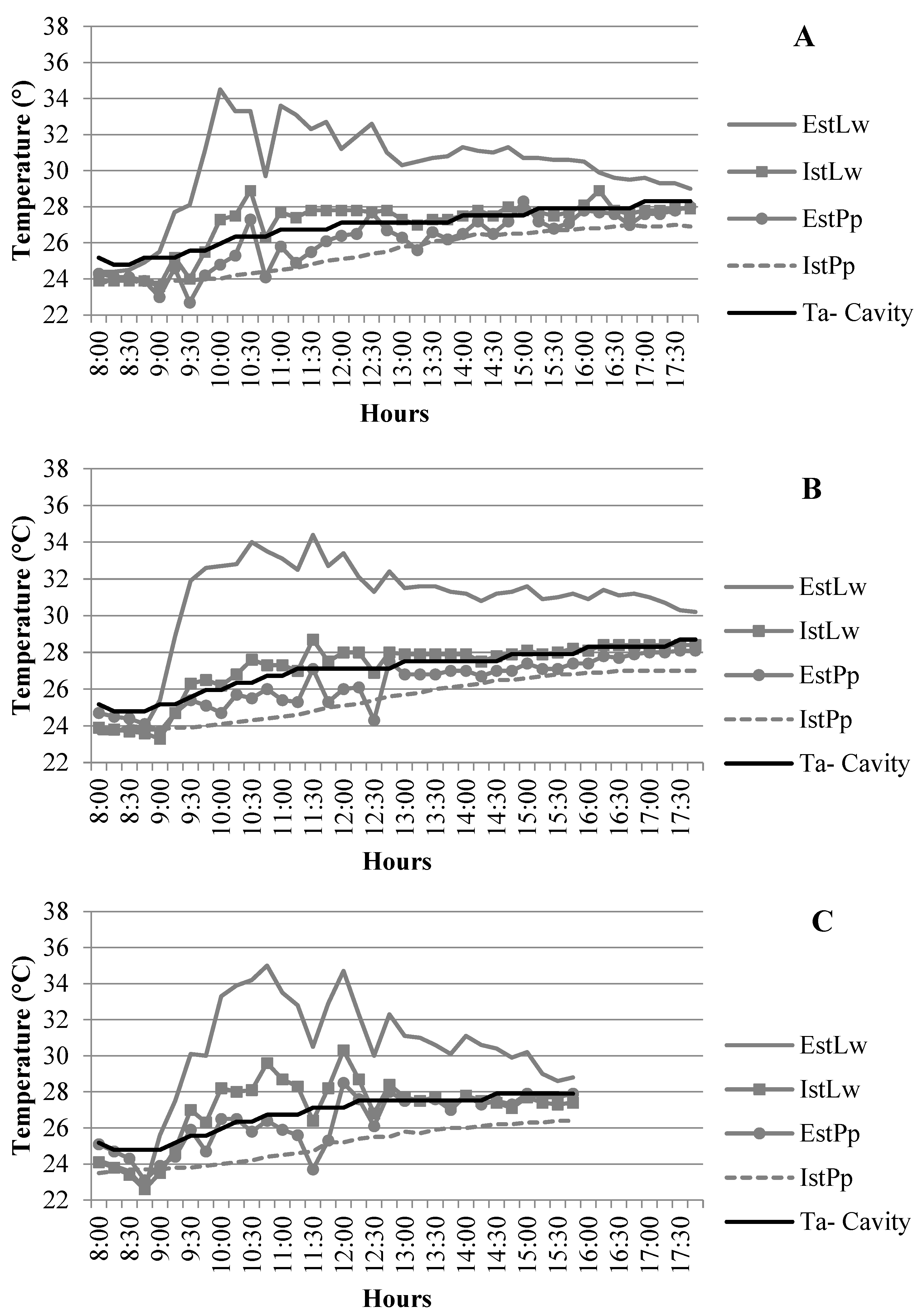
Figure 11 shows the behavior of the monitoring points along the structure of the living wall and the external and internal surfaces of the protected plot in relation to the control plot for the following variables: external surface temperature of the control plot (EstBw), internal surface temperature of the control plot (IstBw), external surface temperature of the living wall (EstLw), internal surface temperature of the living wall (IstLw), external surface temperature of the protected plot (EstPp), and internal surface temperature of the protected plot (IstPp).
The surface temperatures of the “garden-protected plot” system were lower than the EstBw on the 1st day of monitoring and higher on the other days until 8:30 (i.e., the beginning of direct sunlight). From that time on, IstLw, EstPp, and IstPp were lower than EstBw, while they were lower than IstBw from 12:15 until the end of the monitoring period.
With direct sunlight, there was a standardization of the gradient of the surface temperatures of the “garden-protected plot” system in the three days of monitoring. This gradient indicates the heat flow input direction towards the internal environment and is represented by the following sequence: EstLw, IstLw, EstPp, and IstPp.
Surface temperatures varied in pairs; that is, the EstLw varied along with the EstBw, IstLw varied together with EstPp and, finally, IstPp and IstBw varied together. This pattern of variation and thermal gradients demonstrates how the constructive layers of the living wall provide shade, increase the system’s thermal resistance, and prevent the direct influence of solar radiation on the inner surface of the garden and the external surface of the protected plot.
The thermal behavior of EstLw in relation to the bare wall can be explained by its direct exposure to solar radiation, meaning that the garden depends exclusively on the density and distribution of vegetation cover to shade and block the solar incidence on its external surface. Thus, the vegetation in this experiment contributed with maximum reductions of 2.8–3.5 °C in the external surface temperature of the garden in relation to the external surface temperature of the bare wall. On the other hand, the vegetation did not reduce the EstLw variation in the monitoring period; that is, the garden temperature was lower, higher, and at the same degree as the bare wall each day.
The investigation of vegetation cover on the EstLw is not widely discussed in the literature, and only two studies have identified the same thermal behavior of this variable. Wong et al. (2010) [
3] found a reduction of up to 9 °C compared to a concrete control wall. The authors also noted that, in most of their measurements, the values of the garden approached and maintained a daily variation as high as those of the control wall, in the same way as the results registered in this work.
Victorero et al. (2015) [
25] obtained a difference of up to 30 °C between the external surface of the vertical garden and a metallic bare wall. This large difference was related to the characteristics of the materials and the red color of the bare wall, as well as the types of vegetation used by the researchers.
The vegetation constitutes the first shading layer in the system, and contributed to the maximum values of EstLw occurring in the morning (10:00 to 11:30)—an average of 1 h before those of the bare wall. The maximum difference between the temperature peaks was 2.7 °C, and the average difference was 0.7 °C, with the garden surface registering lower temperatures. However, on the 3rd day, the EstLw reached a difference of 0.6 °C higher compared to the bare wall.
Thus, considering that the complete living wall system provided an average difference of 6.9 °C between the temperature peaks (
Table 6) for the EstPp in relation to the EstBw, the shading of the vegetation contributed about 10% of this amount. The vegetation also contributed to anticipating the maximum values of EstLw in relation to the control plot. This behavior has not previously been discussed by any similar studies.
IstLw had generally higher values than EstPp, with a maximum difference of 3.2 °C. From 17:00 onwards, there was a trend towards an increase in EstPp due to the heat flow coming from the living wall system and the thermal exchanges occurring in the air cavity environment. This flow can be identified through the drops in the internal and external surface temperatures of the garden and the simultaneous increase in the external surface temperature of the protected plot.
3.3. Cavity Thermal Exchange System
Heat transfer occurs via conduction throughout the garden structure in the direction of the thermal gradient, and then via radiation (between the external surface of the protected plot and the internal surface of the garden) and via convection (between the garden’s and the protected plot’s surfaces and the cavity air) [
22], contributing to changing temperatures in the air cavity.
To identify these changes, the temperatures of the surfaces were compared to the cavity air temperature in order to verify whether the temperature variations between the internal surface of the garden and the external surface of the protected plot reflected changes in the cavity air temperature (
Figure 12).
It was observed that even with more intense temperature variation between the two surfaces, this variation was not reflected in the cavity air temperature, which continued to show little variation and long periods of stability. That is, at times, when surface temperatures decreased or increased abruptly, there was no consecutive increase or decrease of the same intensity in the air temperature that could occur through convective thermal exchanges between the air and the contact surfaces.
However, there was a relationship between the surface temperature curves, in which, based on variations in the values of the surface temperatures (external and internal) of the garden and the external surface temperature of the protected plot, there was a gradual increase in the internal surface temperature of the protected plot. Thus, it can be inferred that the thermal exchange processes through the “garden-protected plot” system occur more intensely through the conduction and radiation processes, and that radiation is the main thermal exchange process in the air cavity environment between the garden and the protected plot. It is noteworthy that the air cavity was sealed by the constructive structure in order to prevent convection with the external air, as described by Chen et al. (2013) [
22].
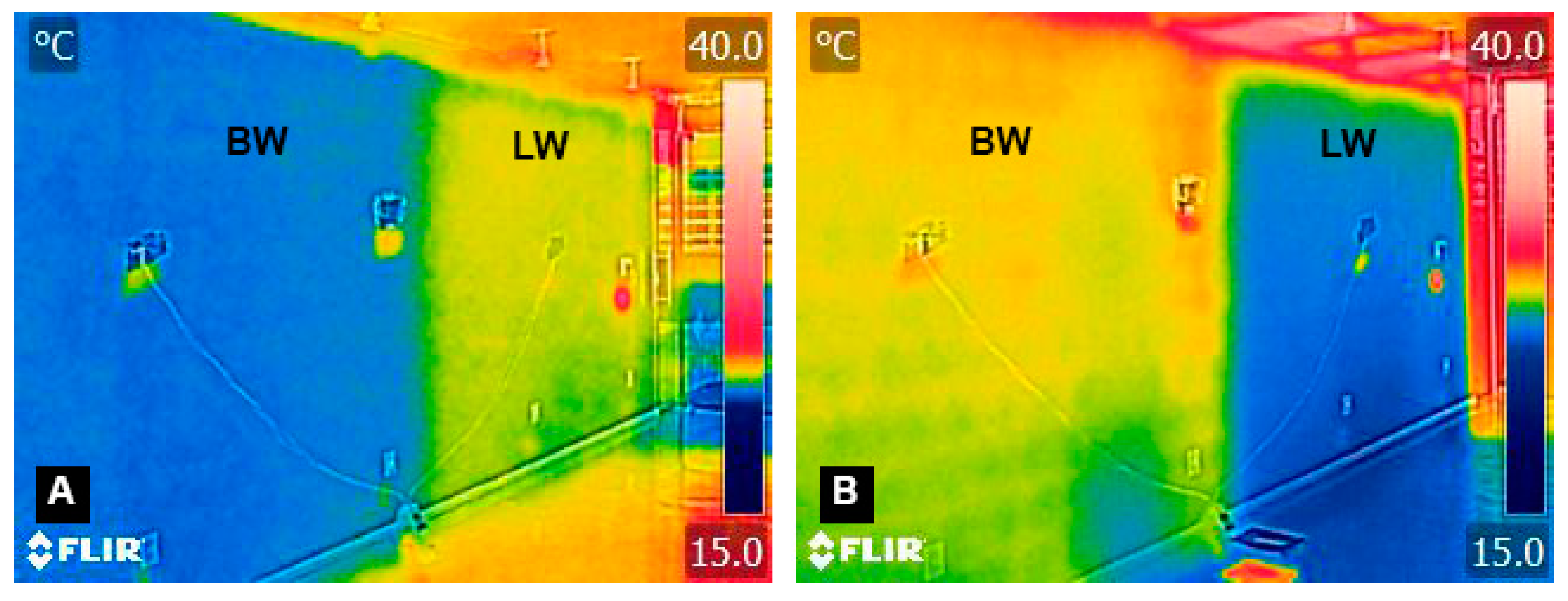
The dynamics of this heat flow and the insulation created by the living wall over the protected plot, preventing the entry of heat into the internal environment, can be visually identified as shown in
Figure 13. At the beginning of the monitoring, the internal surface of the protected plot started with more heat; however, with the incidence of direct solar radiation, an inversion occurred, and the control plot started to present the most heated surface until the end of the measurement period.


