Long-Term Scenario Analysis of Electricity Supply and Demand in Iran: Time Series Analysis, Renewable Electricity Development, Energy Efficiency and Conservation

Abstract

Electricity plays a vital role in the economic development and welfare of countries. Examining the electricity situation and defining scenarios for developing power plant infrastructure will help countries avoid misguided policies that incur high costs and reduce people’s welfare. In the present research, three scenarios from 2021–2040 have been defined for Iran’s electricity status. The first scenario continues the current trend and forecasts population, electricity consumption, and carbon dioxide emissions from power plants with ARIMA and single and triple exponential smoothing time series algorithms. As part of the second scenario, only non-hydro renewable resources will be used to increase the electricity supply. By ensuring the existence of potential, annual growth patterns have been defined, taking into account the renewable electricity generation achieved by successful nations. The third scenario involves integrating operating gas turbines into combined cycles in exchange for buyback contracts. Economically, this scenario calculates return on investment through an arrangement of various contracts for the seller company and fuel savings for the buyer.

1. Introduction

In recent decades, electricity demand has risen due to the growth of population, urbanization, and industrialization of nations. Due to the ever-increasing demand for electricity, primary resources are consumed at an increasing rate, resulting in environmental concerns and fossil fuel depletion. Meanwhile, no one can deny how crucial electricity is to economic development and welfare. In this context, the mission of policymakers is to guide countries towards better electric generation capabilities and utilization of less polluting resources following their electricity needs. Inappropriate programs might cause irreparable economic or environmental damage to a country, affecting its residents’ lives. Evaluating electricity status and analyzing electrical infrastructure development under various scenarios can assist in formulating appropriate long-term plans.

There have been many studies conducted this way. Mirjat et al. [1] have defined four scenarios for the electricity situation in Pakistan in 2015–2050: a reference scenario; renewable electricity (RE) development; efficient technology development for electricity generation; and energy conservation and reduction of demand. Net present value and emissions are assessed in each of these scenarios. The term “Reference” or “Business-as-Usual” (BAU) refers to scenarios where policies and programs are supposed to be continued in the same manner. Generally, all energy-related scenario studies involve the BAU scenario. Moreover, scenario studies can be classified based on their forecasting horizon: intra-hour-, (sub-hourly), short- (daily), mid- (monthly), and long-term (yearly) forecasting [2]. In another study, Liang et al. [3] examined three scenarios for Chinese electricity development: BAU, RE development, and increasing capacity factor. Iran has also been the subject of similar research. Sabeti Motlagh et al. [4] defined seven scenarios for Iran’s electricity supply and demand within 2011–2030: BAU; a removal of subsidies and an increase in electricity prices; conversion of steam power plants to a combined cycle (CC); distributed generation of electricity; development of advanced combustion power plants; use of carbon capture systems; conversion of gas turbine (GT) power plants to CC; and a combined scenario are set out in the studies. In another study, Masoomi and colleagues [5] set out three scenarios for Iran’s electricity situation through 2013–2035. The BAU is the first scenario. In the second scenario, an annual increase of 1% in the total efficiency of the country’s thermal power plants is assumed. This percentage has been approved in the five-year development plan of Iran. In the third scenario, the efficiency of thermal power plants in the UK is considered Iran’s goal. The quantities investigated in this study are limited to fuel consumption, environmental emissions, and environmental costs. In another study, Masoomi et al. [6] set up more scenarios. In one scenario, by changing electricity consumption patterns in the residential sector and reducing transmission and distribution losses, a 5% reduction by 2035 is considered. In addition, they evaluated the environmental costs by defining several simple scenarios. Each scenario was dedicated to each gas, steam, and diesel turbine as well as to CC technologies. In addition, Kachoee et al. [7] examined three scenarios from 2011 to 2040 regarding the electricity situation in Iran. Their first step was to analyse a BAU scenario with approximate assumptions. The second scenario involved integrating GT power plants into CC and installing thermal power plants that consume less fuel and emit fewer pollutants. In the third scenario, the development of renewable power plants, especially hydroelectric power, the conversion of GT power plants to CC, the development of nuclear power plants, and the consumption of natural gas fuel were envisioned as the goals of this scenario.

Although numerous electricity scenarios have been analyzed for Iran, the majority of the applied scenarios are based on older data. Additionally, the studies conducted are based on the legal structure of the country, but historical evidence indicates that Iran’s energy indicators have not followed its laws. Hence, time series algorithms are better suited for predicting Iran’s future than traditional scenarios. In terms of forecasting the BAU scenario, a variety of algorithms are being used. Jamil et al. [8] used an autoregressive integrated moving average (ARIMA) model based on the historical data of the past 53 years to forecast the hydroelectricity consumption of Pakistan until 2030. It was validated that the forecasted values were accurate by comparing them with the actual values, which showed a good fit with minimum deviation. Adjusted R2 was presented and used to calculate the accuracy of the model, amounting to 0.288–0.324. Xue et al. [9] proposed an option contract model with the help of daily electricity price data from 2017 to 2019 from the Nord Pool exchange system. They used the ARIMA model to predict this price index and model parameters. The mean absolute percentage error (MAPE) amounts to 5.55%. Nafil et al. [10] proposed mid-term energy forecasts to clarify energy demand growth based on three forecasting methods (ARIMA, temporal causality modeling, and exponential smoothing (ES)). The aim of this is to calculate energy demand forecasts for Morocco in 2020. The R2 score of the developed ARIMA model accounted for 0.903. De Oliveira et al. [11] proposed a hybrid model based on ES and bagging ARIMA to forecast mid–long-term electricity consumption on a monthly scale. Based on the results of the proposed methodologies, both developed and developing countries achieve substantial improvements in forecasting accuracy for energy end-use services. The MAPE of the developed auto-ARIMA model amounts to 5.14. Kim et al. [12] presented a hybrid model consisting of seasonal ES to predict the short-term electricity load for institutional buildings. The peak load demand of an institutional building in Seoul was forecasted. The datasets are related to the campus area of 23 buildings. They used the weather and holiday variables for prediction since these are crucial. The MAPE of the developed ARIMA and triple ES (Holt) models were calculated at 2.28–12.01 and 2.75–11.09, respectively.

As aforementioned, almost all scenarios applied to Iran are based on older data. Furthermore, in comparison to traditional scenario planning based on legal structures, time series algorithms might be more effective at predicting Iran’s future. Accordingly, in the present research, three scenarios are analyzed between 2021 and 2040 to evaluate resource management in Iran in terms of electricity production. In the first scenario, the continuation of the existing trend in the key indicators included population, electricity consumption, and carbon dioxide (CO₂) emissions from power plants, forecasted by time series algorithms. The second scenario states that electricity generation developments must be exclusively renewable in the future. In this scenario, the potential of Iran in various resources is compared with other countries. In the third scenario, the conversion of GT power plants to CC is economically analyzed. In this regard, a comprehensive cost analysis is conducted.

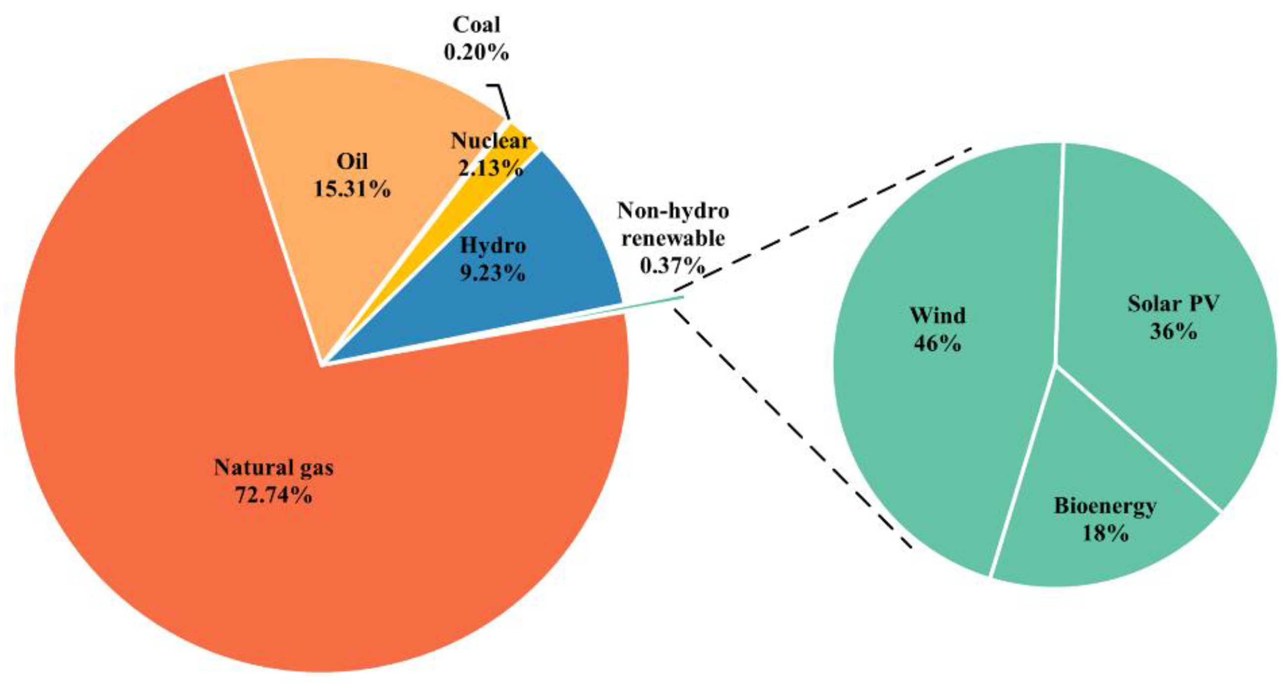
2. Iran Energy Structure

Iran occupies a land area of 1,628,760 km³ and has a population of 84 million. It is reported that Iran’s GDP is $230 billion, and its HDI is also 0.774 [13,14]. Regarding energy resources, fossil fuels are plentiful in Iran. Proven oil and gas reserves include 32.1 trillion cubic meters and 157.8 billion barrels, accounting for 17.1 and 9.1% of global reserves. Among all the countries in the world, Iran ranks second in gas reserves, fourth in oil reserves, and first in their total reserves [15]. In some cases, these fields are shared by neighbors, e.g., the world’s largest gas field, South Pars, is located cooperatively in Iran and Qatar’s territorial waters in the Persian Gulf [16]. In this field, both countries use non-conservative approaches. The reason is that if one country extracts less oil and gas the other country gains access to those resources [17]. Due to the abundance of fossil fuels, a large proportion of electricity is generated using those fuels. Natural gas accounts for 72.7% of electricity production and oil for 15.3%, resulting in 88.1% of electricity being generated from fossil fuels [18]. Figure 1 shows the electricity generation mix of Iran.

Iran’s non-renewable energy policy emphasizes the development of GT power plants that can be combined with the steam cycle to maximize productivity. During 1997–2019, the country’s power plants’ efficiency increased from 30.5% to 37.6% [19]. Regarding RE, there is a growing interest in RE from the Iranian government. Efforts are being made by the Iranian government to increase investment in RE. The sixth Five-Year National Development Program targets 5% RE generation by 2022, although current statistics indicate a gap in achieving the target.

3. Theory and Methods

In the present research, three scenarios are defined for Iran. A summary of the scenarios is shown in

Table 1. Overview of the scenarios defined for Iran’s electricity sector.

Scenario	Objective	Method
Trend continuation	The current trend is followed.	Time series algorithms
Renewable electricity development	Future electricity generation developments are exclusively renewable.	Historical data of developed countries
Energy efficiency and conversion	All active gas turbine power plants are integrated into combined cycles.	Economic and environmental analysis

.

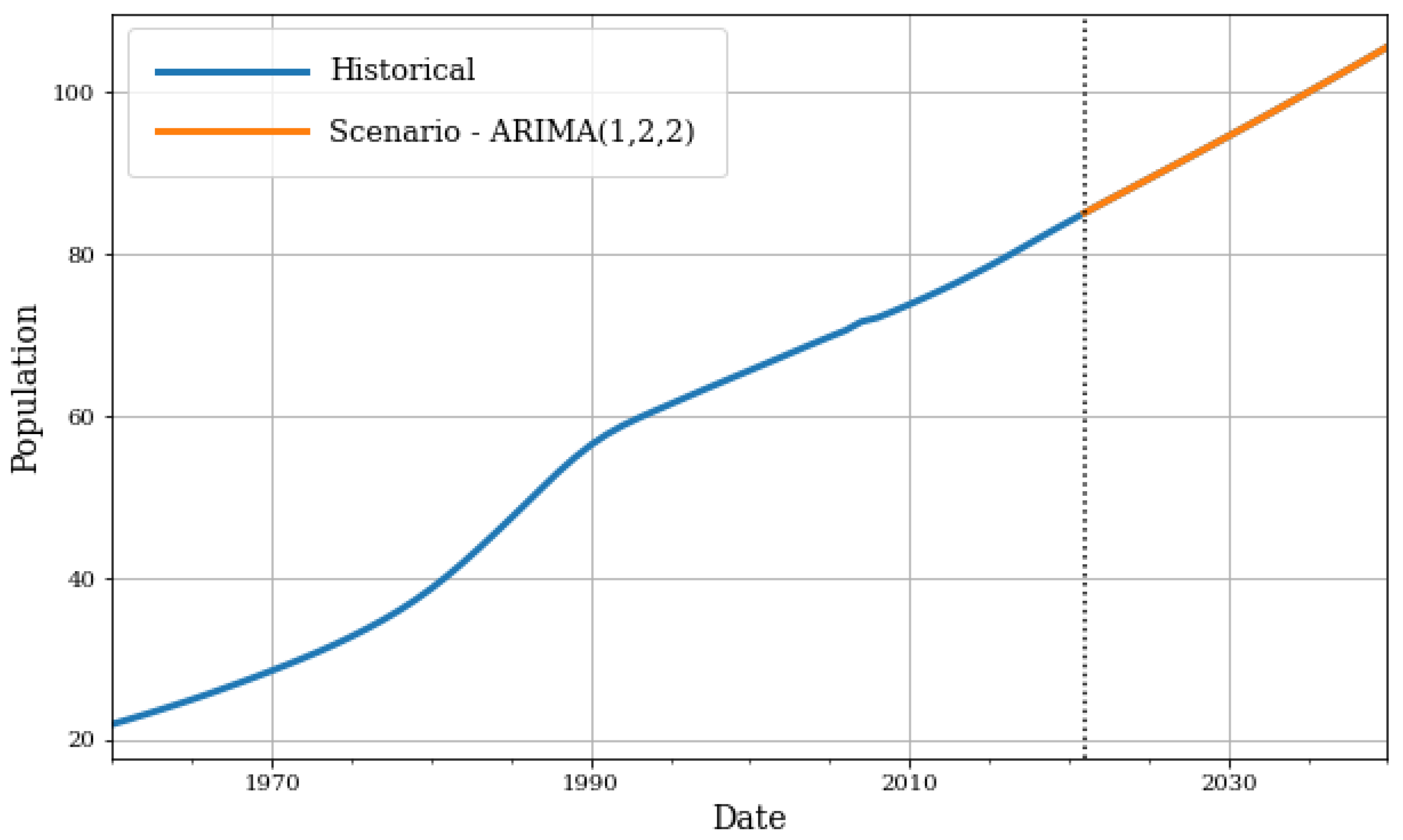
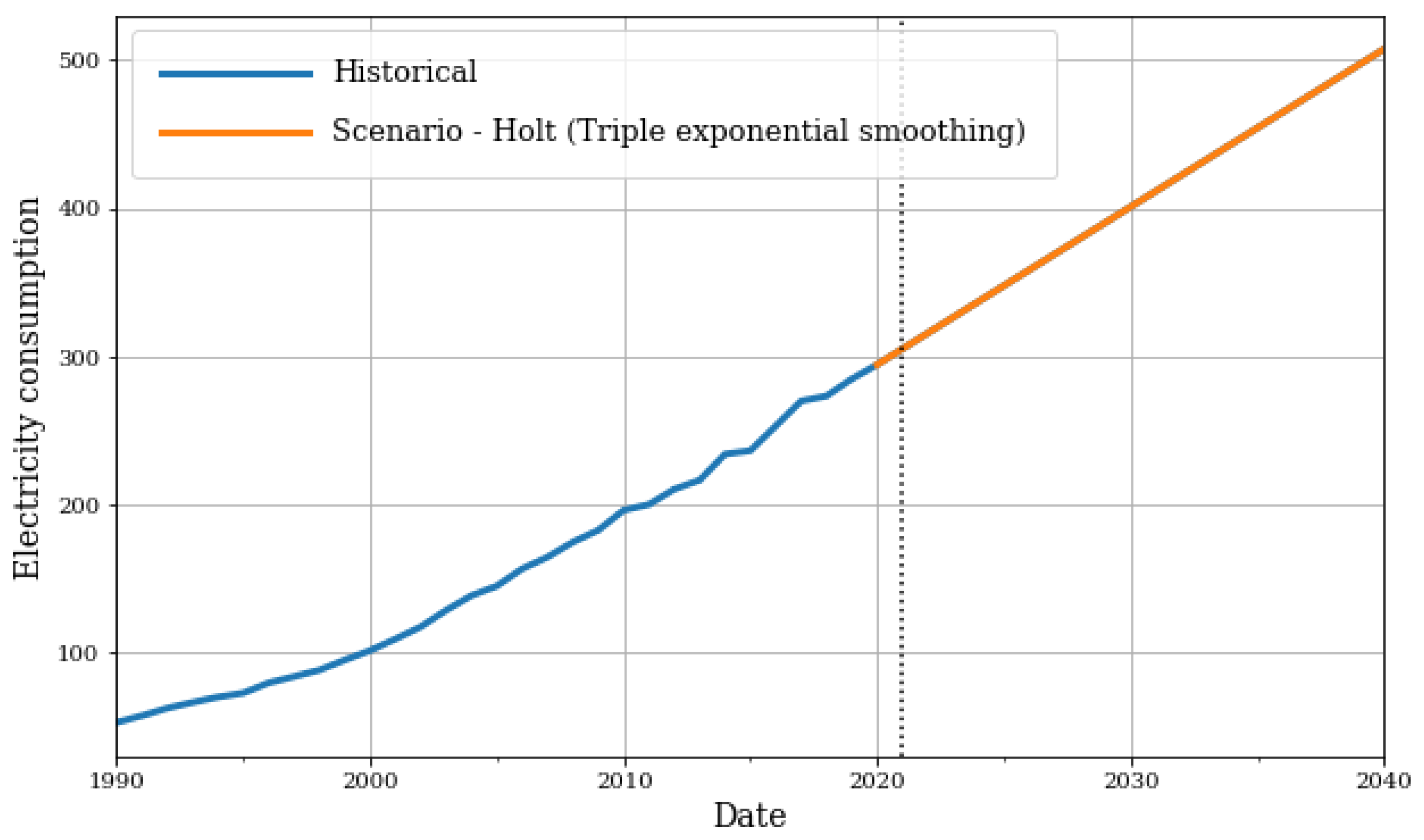
3.1. Trend Continuation

In this scenario, the following question is addressed: “If the current trend continues, what will happen to the power plant complex in Iran?” Iran’s electricity generation has been investigated from the standpoints of consumption and emissions, and it will be determined what can be expected of the country’s power plants over the next 20 years. Important energy indicators have been assessed and calculated through classic time series algorithms including single ES (SES), Holt, and ARIMA. The indicators include population, electricity consumption, and CO₂ emissions from power plants.

A time series is a collection of data that is recorded and specified in time order at equal intervals. The analysis of these data is divided into two stages. In stage one, the data’s structure and pattern are determined, and, in stage two, the model is fitted to predict future trends. The time series models can be univariate or multivariate. In contrast to a univariate dataset, a multivariate dataset contains multiple time-dependent variables [20,21,22]. The most-known time series algorithms include:

• Classical statistical linear time series, e.g., autoregression (AR), moving average (MA), ARIMA, ES;
• Non-linear time series, e.g., generalized autoregressive conditional heteroskedasticity (GARCH), autoregressive conditional heteroskedasticity (ARCH);
• Time series with supervised machine learning, e.g., Bayesian, decision trees, support vector machines (SVM);
• Time series with deep learning, e.g., long short-term memory (LSTM), RNN, convolutional neural networks (CNN), feed-forward neural networks (FNN).

Considering the number of predictions and the non-seasonality of the collected data in the present research, we need to use a simple, fast, accurate, and inexpensive method. Hence, the ARIMA and ES methods are chosen to forecast current trend continuation. It should be noted that the analysis is performed using the “statsmodel” library in Python.

3.1.1. ARIMA

The ARIMA algorithms include autoregression (AR), moving average (MA), autoregressive moving average (ARMA), ARIMA with exogenous variables (ARIMAX), seasonal ARIMA (SARIMA), and seasonal ARIMAX (SARIMAX).

They were introduced by Box and Jenkins. This method includes model identification, parameter estimation, and a diagnostic investigation followed by forecasting [22]. To make forecasts, several steps are taken [23,24,25,26]:

Preprocessing: This prepares the collected data for use in training predictive models, which can include checking the number of observations, filling in missing data, rescaling, and separating training and testing data. In the present case study, the data were collected annually from 1960 to 2020 for the population and from 1990 to 2020 for the electricity consumption and CO₂ emissions from power plants. The data were gathered from Iran energy balance sheets [19], IEA [18], and the World Bank [13]. Furthermore, 20% of the data are split as test data to evaluate the models’ accuracy.

Checking data stationarity: A stationary time series is one in which autocorrelation decreases with increasing lag. For non-stationary data, the mean, variance, and covariance are not time-dependent; thus, they are unpredictable and cannot be modeled or forecasted. In this case, data must be transformed into stationary data. Differencing is one of the ways of converting non-stationary data into stationary data. Differenced series (y_t−y_t−1) are the changes between consecutive observations in the original series. It might be necessary to perform two or more steps of differencing if the data are not stationary after one step of differencing. To check data stationarity, the Dickey–Fuller test, autocorrelation function (ACF), and partial autocorrelation function (PACF) plots are commonly used. In the present study, the AD Fuller test, which is an upgraded version of the Dickey–Fuller Test, is utilized to determine whether the data are stationary or not.

Checking data seasonality: Seasonality represents periodic, repetitive, and generally regular and predictable patterns of a fixed and known period (day, week, month, etc.) that occur at specific regular intervals. By decomposing a time series into trend, seasonal, and residual components using “seasonal decompose” in Python, it is possible to analyze the features and structure of variations occurring over time. A multiplicative or additive decomposition method is used to determine seasonality. Since our data in this paper were collected annually, there is no seasonality; thus, seasonality-related models such as SARIMA and SARIMAX are not used.

There are three terms in an ARIMA model: p, d, and q, where p is the order of the AR term, q is the order of the MA term, and d is the order of the differencing required to make the time series stationary. For stationary data, the value of d is set to zero and the model becomes an ARMA model. For seasonal data and also non-stationary data, the SARIMA(p,d,q)(P,D,Q)m model is used, in which P is the seasonal AR order, D is the seasonal difference order, Q is the seasonal MA order, and m is the number of time steps (lags) for a single seasonal period [27]. Using AR, forecasts would be implemented by the previous values of observations. However, in MA, errors associated with the forecast at a previous time step are used to forecast the variable at a later time step. Generalized equations for AR (p) and MA (q) models are given below [25,28]:

$$y_t=k+{\varnothing }_1{y}_{t-1}+{\varnothing }_2{y}_{t-2}+\dots +{\varnothing }_p{y}_{t-p}+{\epsilon }_t$$

(1)

$$y_t=k+{\epsilon }_t+{\theta }_1{\epsilon }_{t-1}+{\theta }_2{\epsilon }_{t-2}+\dots +{\theta }_q{\epsilon }_{t-q}$$

(2)

The ARIMA model is constructed by incorporating the AR model (Equation (1)), the integration (I), and the MA model (Equation (2)). The integration is the reverse process of differencing to generate the forecasts. In mathematical terms, the generalized ARIMA model can be expressed as Equation (3) [25,28].

$$y_t=k+{\varnothing }_1{y}_{t-1}+{\varnothing }_p{y}_{t-p}+\dots +{\theta }_1{\epsilon }_{t-1}+{\theta }_q{\epsilon }_{t-q}+{\epsilon }_t$$

(3)

In Equations (1)–(3); ${\varnothing }_1$, …, ${\varnothing }_p$ are AR model parameters; k is a constant; θ₁, …, θ_q are MA model parameters; and ε_t, ε_t−1, and ε_t−q are white noise error terms.

Order selection: As mentioned, d is the number of differences required to be taken to convert the data into stationary data. Detecting patterns and checking for randomness can be accomplished with autocorrelation analysis. In ARIMA and ARMA, q is determined using ACF and p is determined using PACF. ACF gives the values of autocorrelation between a series and its lagged values. In other words, ACF is a way to measure the linear relationship between an observation at time t and observations at previous times. PACF provides the partial correlation between a stationary series and its own lagged values. The working method is that in every lag where the value exceeds the significance threshold (significance level), it has the potential to be selected for the desired order. Depending on the field of study, the significance threshold may be 0.01, or even 0.001. Researchers often use p-values to determine whether a pattern they have measured is significant. Likewise, in this research, ACF and PACF are examined, and the models are fitted to the training data by selecting appropriate orders based on their p-values (which should be less than 0.05). Moreover, we examined two information criteria, the Akaike information criterion (AIC) and the Bayesian information criterion (BIC), allowing us to impose a small penalty on the number of parameters or test how well the model fits the dataset without overfitting [29,30]. These values are calculated by [25,30,31]:

$$\mathrm{AIC}=-2\log L\left(\widehat{V}\right)+2N_e$$

(4)

$$\mathrm{BIC}=-2\log L\left(\widehat{V}\right)+N_e\log N_o$$

(5)

where V is the set (vector) of model parameters, L($\widehat{V}$) is the maximum value of the likelihood function of the model, N_e is the number of estimated parameters in the candidate model, and N_o is the number of observations. Models with a lower AIC and BIC have a better fit.

The method described earlier can be time-consuming when selecting the best parameter (p, d, q) manually, as the number of models to evaluate depends on the number of model order parameters, and can consume more even when selecting the parameters for SARIMA(p,d,q)(P,D,Q)m. A smarter way to choose the appropriate combination of model parameter values is to use auto-ARIMA, which is available in the “pmdarima” library in Python [25].

Normality test for residuals: This step is taken by plotting the distribution diagram of the residuals for the model. The zero mean normal distribution indicates the appropriateness of the selected model [32]. Additionally, ACF and PACF plots for residuals indicate an appropriate model if all lag values are within the significance level. Figure 2 is given as an example to show this step. This figure includes the KDE plot, ACF, and PACF plots for residuals of an ARIMA(1,2,2) model that is used to forecast the population of Iran.

Accuracy evaluation: For this purpose, different evaluation metrics can be used on the test data [21]. In this article, MAPE and mean squared error (MSE) are used to evaluate the accuracy of the model. Equations (6) and (7) are the respective formulae for MAPE and MSE [21,33,34].

$$\mathrm{MAPE}=\frac{1}{N_{te}}{\displaystyle \sum }_{\mathrm{t}=1}^{N_{te}}\frac{\left|y_{forecaste{d}_t}-y_{actua{l}_t}\right|}{y_{actua{l}_t}}\times 100\%$$

(6)

$$\mathrm{MSE}=\frac{1}{N_{te}}{\displaystyle \sum }_{t=1}^{N_{te}}{\left(y_{forecaste{d}_t}-y_{actua{l}_t}\right)}^2$$

(7)

where N_te represents the total number of test data.

Forecasting: As the final step, the future values could be forecasted by the fitted model. Figure 3 shows the workflow of the general procedure for using ARIMA models.

3.1.2. Exponential Smoothing

Through the ES algorithm, a weighted average of past values is used to calculate the upcoming values in this method. The older a value, the lesser the weight assigned to it. Over time, the ES has undergone modifications.

Table 2. Predictability of exponential smoothing methods.

Exponential Smoothing	Level	Seasonality	Trend
Simple exponential smoothing	✓	✓	-
Double exponential smoothing	✓	-	✓
Triple exponential smoothing (Holt)	✓	✓	✓

shows the predictability of various ES methods [35].

Holt formulae are given by Equations (8)–(11). The forecasted value m periods ahead can be calculated by [36]:

$$y_{t+m}=s_t+m{b}_t+c_{t-L+1+\left(m-1\right) mod L}$$

(8)

where s_t represents the smoothed observation, b_t is the trend factor, c_t is the seasonal index, and L refers to the length of the seasonal change cycle. s_t, b_t, and c_t are given by [36]:

$$s_t=\alpha \left(y_t-c_{t-L}\right)+\left(1-\alpha \right)\left(s_{t-1}+b_{t-1}\right)$$

(9)

$$b_t=\beta \left(s_t-s_{t-1}\right)+\left(1-\beta \right)b_{t-1}$$

(10)

$$c_t=\gamma \left(y_t-s_{t-1}-b_{t-1}\right)+\left(1-\gamma \right)c_{t-L}$$

(11)

where y_t represents the observation. α refers to the data smoothing factor, β is the trend smoothing factor, and γ is the seasonal change smoothing factor. α, β, and γ are the hyperparameters between 0 and 1 and must be estimated to minimize the error [36]. The hyperparameters are measured by a trial-and-error process and by continuously calculating the MAPE and MSE.

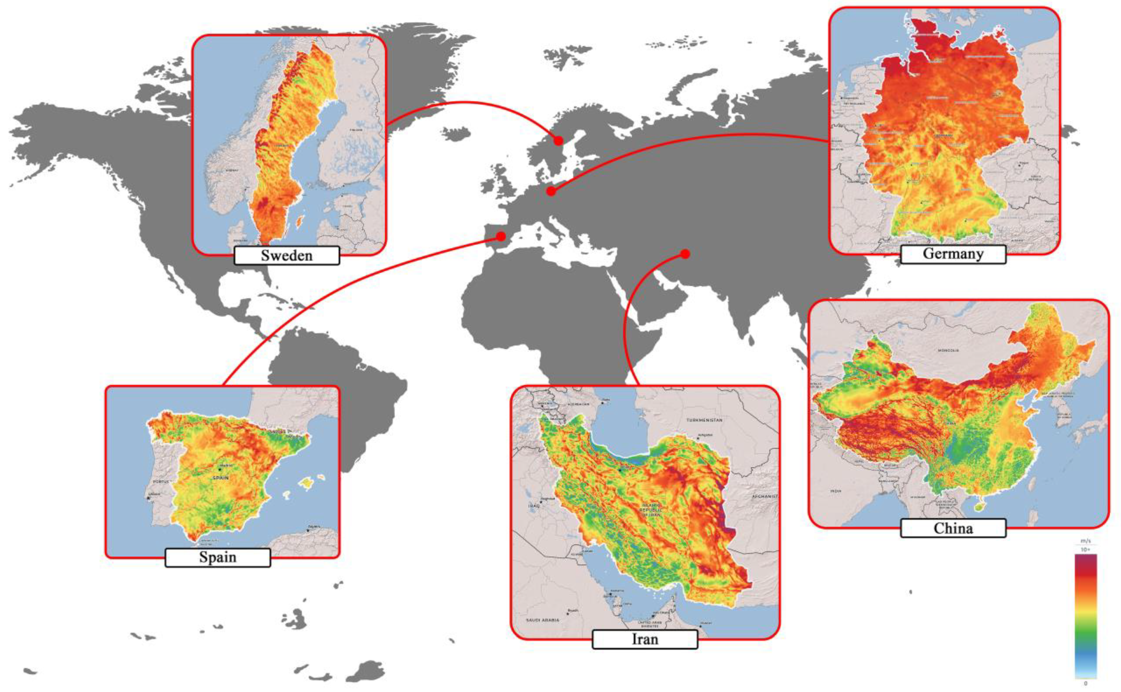
3.2. Renewable Electricity Development

Nowadays, one of the top priorities for developed countries is environmentally friendly methods to generate electricity, especially renewable energy. Among RE resources, hydropower is by far the largest in the world, with a capacity of 1328 GW [18]. However, in recent years, due to severe drought conditions, hydropower plants have had much less actual capacity than their nominal capacity [18]. Despite the water crisis, hydropower is expected to lose popularity in the coming years, as is its share of electricity generation. After hydropower, solar and wind energy have the world’s largest electricity generation capacity among renewables, with amounts of approximately 745 and 740 GW, respectively. Solar energy has the greatest potential to meet the world’s electricity requirements in the future, accounting for 60% of all renewable capacity additions [18]. Iran has vast potential for the utilization of renewable energy, including wind, solar, geothermal, bioenergy, and ocean energy.

In this scenario, the development of RE in Iran has been analyzed. The potential of each RE resource has been explored in Iran and several developed countries including Germany, China, Spain, Sweden, and the UK. In these countries, renewable energy has been used to produce electricity for a long time. In addition, countries like Iran, which are transitioning to RE, might have similar patterns of development to these countries, although their resources should also be considered. For this purpose, the annual growth of per-capita electricity production by resource in the last 20 years is calculated for each of these countries. By comparing Iran’s potential with these countries, the annual growth of per-capita electricity production in each of these resources has been introduced as the expected trend for Iran in the next 20 years. Then, the production targets for each resource in 2040 are calculated. The resources include photovoltaics (PV), wind, geothermal, liquid biofuels, municipal waste, biogas, primary solid biofuels, industrial waste, and tide. It should be noted that electricity generation from fossil, nuclear, and hydro resources is planned until the end of 2040 without change. In addition, the population of Iran in 2040, which is obtained by the trend continuation scenario, is a criterion for calculating the amount of production capacity.

3.2.1. Photovoltaics

The potential for generating electricity from PV in Iran is much higher than in other countries (Figure 4). Detailed statistics are provided in

Table 3. Potential and generation statistics for PV electricity in Iran, Spain, Germany, and China [18,37].

	Spain	Germany	China	Iran
Specific PV power output (kWh/kWp/day)	3.08–4.91	2.32–3.24	2.21–5.82	3.31–5.48
Specific PV power output for the 10% sunniest area (kWh/m2/day)	4.66	3.17	4.98	5.28
Specific PV power output for the 25% sunniest area (kWh/m2/day)	4.59	3.03	4.62	5.11
PV electricity generation (GWh, 2020)	15,552	50,600	269,718	435
Annual growth of PV electricity generation per capita (kWh/capita/year, 2000–2020)	16.40	30.39	9.56	- *

* These calculations are used to model Iran’s renewable electricity development; thus, calculations of this parameter are not necessary for Iran.

[37]. Given Iran’s high potential for generating PV electricity and the maturity of the PV technology, it is expected that great progress could be made in utilizing this resource. Consequently, Iran’s 2040 target is supposed to be similar to Germany’s PV generation, the country generating the highest PV electricity [18].

3.2.2. Solar Thermal

Among the countries whose radiation statistics were examined, Iran and Germany have not used it to generate electricity thus far. However, China and Spain generated 4992 and 1317 GWh in 2020, respectively. In terms of solar thermal energy, Spain’s development has been used to predict Iran’s.

Table 4. Solar thermal electricity generation in Spain and China [18].

	Spain	China
Solar thermal electricity generation (GWh, 2020)	4992	1317
Annual growth of solar thermal electricity generation per capita (kWh/capita/year, 2000–2020)	5.27	0.05

provides detailed statistics [18].

3.2.3. Wind

Iran’s wind energy potential, especially in the eastern regions, is very high, but it produces far less electricity than most other countries (Figure 5). More detailed information on wind power generation is given in

Table 5. Potential and generation statistics for wind electricity in Spain, Germany, China, Sweden, and Iran [18,38].

	Spain	Germany	China	Sweden	Iran
Mean power density for the 10% windiest area (W/m2)	716.56	594.96	668.89	742.92	743.75
Mean power density for the 20% windiest area (W/m2)	582.80	543.62	556.26	591.82	602.63
Wind electricity generation (GWh, 2020)	56,273	130,965	471,175	27,526	555
Annual growth of wind electricity generation per capita (kWh/capita/year, 2000–2020)	53.58	73.05	16.67	130.40

. In light of Iran’s high potential, Spain was chosen as a trend model [18].

3.2.4. Geothermal

Similarly, geothermal energy may also be a high-energy-potential area for Iran, but the country has not developed any productivity in this field, except for traditional medicine and tourism applications. Following studies conducted by the Renewable Energy and Energy Efficiency Organization (SATBA), the volcanic regions of Meshginshahr can also be used to build 400 MW power plants [18]. The potential of Iran extends beyond Meshginshahr. Iran has high geothermal potential in 8.8% of its area, including 18 promising fields, which require comprehensive geochemical, geophysical, and geological assessments [39]. The generation of geothermal electricity in Germany and China is summarized in

Table 6. Geothermal electricity generation in Germany and China [18].

	Germany	China
Geothermal electricity generation (GWh, 2020)	217	125
Annual growth of geothermal electricity generation per capita (kWh/capita/year, 2000–2020)	0.13	0.00

. As a target in 2040, China’s growth is chosen for Iran’s [18].

3.2.5. Tide

Using tides as a source of electricity is not common among the countries of the world, and there is only 500 MW of electricity generation capacity worldwide. South Korea, France, the UK, China, Russia, and the Netherlands generate electricity sporadically using this resource. Technology using tidal and ocean resources has not yet matured, but, if it is developed, the potential for ocean energy worldwide is said to be greater than the global need for electricity [40]. The Caspian Sea borders Iran in the north and the Oman Sea and the Persian Gulf in the south, allowing it to access tide energy. This allows developments to take place. Consequently, a target of China’s growth is chosen for Iran in 2040, because of its lesser amount.

Table 7. Potential and generation statistics for tidal electricity in China and the UK [18,41].

	China	UK	Iran
Length of shorelines (km)	14,500	12,429	3200
Tidal electricity generation (GWh, 2020)	12	11	-
Annual growth of tidal electricity generation per capita (kWh/capita/year, 2000–2020)	0.00	0.01	-

points to more energy data on tidal electricity generation [18].

3.2.6. Bioenergy

The agricultural economy plays an imperative role in Iran, making up a significant part of its economy. Around one-third of Iran’s land is agricultural, and 17.6% of the Iranian labor force was employed in agriculture in 2017. Iran has also established a significant animal husbandry industry, and its infrastructure has improved substantially. As a result, the industry’s face has been dramatically transformed, in such a way that the entire supply chain process is carried out in the country itself. The annual potentials for agricultural, livestock, and urban waste are about 8.78, 7.7, and 3 Mt [42]. A wide variety of energy crops can be grown in Iran thanks to its land and climate. Sugarcane and sugar beet, which are raw materials for biofuel production in Iran, are cultivated. Around 17.86 Mt of crop wastes are generated every year, which can produce nearly 5 billion liters of bioethanol. In addition, forests cover about 7% of the land in Iran, which provides an excellent source of liquid biofuels, such as bioethanol and biodiesel. Furthermore, Iran has a very high fishing potential, with roughly 3200 km of shorelines and rivers. Fish oil and other vegetable oils, such as date palm, jatropha, castor plant, and algae are the raw material for biodiesel. Around 20% of the 1.5 Mt of edible oil consumed in Iran each year can be considered waste, making it a suitable feedstock for biodiesel production [18].

Based on existing interpretations of Iran using bioenergy resources to generate electricity, it could be a global leader; however, electricity production in Iran is negligible and limited to biogas.

Table 8. Electricity generation by type of bioenergy in Spain, Germany, China, Sweden, and Iran [18].

	Spain	Germany	China	Sweden	Iran
Electricity generation by type of bioenergy (GWh, 2020)
Liquid biofuels	12	383	-	9	-
Municipal waste	686	5811	-	1767	-
Biogas	847	33,041	-	12	22
Primary solid biofuels	4099	11,327	113,961	7649	-
Industrial waste	344	772	10,301	39	-
Annual growth of electricity generation per capita by type of bioenergy (kWh/capita/year, 2000–2020)
Liquid biofuels	0.01	0.23	-	0.04	-
Municipal waste	0.31	2.37	-	8.00	-
Biogas	0.50	18.84	-	−0.12	-
Primary solid biofuels	3.29	6.32	3.94	14.57	-
Industrial waste	0.03	−1.94	0.37	−0.38	-

provides brief information on bioenergy production by type of resource. Here, Spain’s growth pattern is used for resources including industrial and municipal wastes as well as liquid biofuels. Additionally, Sweden’s is used for primary solid biofuels, and Germany’s for biogas.

3.3. Energy Efficiency and Conservation

GT power plants waste a large amount of heat by releasing it into the air or water when not in further use. Addition of the Rankine steam cycle, which produces electricity using the waste heat of the GT power plant, is one of the major measures that can be taken in the field of power generation for GT power plants. Integrating GT units into CC increases power generation capacity without using more fuel and thus brings significant economic and environmental benefits. In this scenario, a seller company will integrate all GT power plants in Iran into CC at its own expense. Iran also undertakes to pay a specific percentage of the income from the sale of electricity to the company through the agreed years. In this manner, Iran develops its energy infrastructure, and the seller makes a high profit. In addition, Iran benefits from the sale of electricity for which fuel is not consumed and avoids a cost equivalent to the price of the saved fuel. This kind of agreement is known as a “buyback contract”. The third scenario focuses on the feasibility of energy efficiency enhancement and presents an economic analysis concisely.

In the first step, it should be calculated how much the nominal capacity will be increased by integration of GT power plants into CC. Therefore, it is necessary to evaluate the efficiency of each of these systems.

Table 9. Actual capacity and efficiency of Iran’s gas turbine and combined-cycle power plants owned by the government of Iran and the private sector [19].

System	Owner	Actual Capacity (MW)	Average Efficiency (%)
Gas turbine	Government	5291	28.9
	Private sector	11,544	33.5
Combined cycle	Government	4397	44.7
	Private sector	17,670	45.2

shows the actual capacity and efficiency of active GT and CC power plants owned by the government of Iran and the private sector.

The total average efficiency of each system can be calculated by:

$$\eta =\frac{P_a^G{\eta }^G+P_a^P{\eta }^P}{P_a^G+P_a^P}$$

(12)

where P_a is the actual power and the superscript G and P point to the government and private sector. Nearly 30% of the total capacity of Iran’s power plants—owned by both the government and the private sector—belongs to GTs, accounting for a nominal capacity of 26,180 MW [19]. The increased nominal capacity of power can be calculated by:

$$P_n=P_n^{GT}\left(\frac{{\eta }^{CC}-{\eta }^{GT}}{{\eta }^{GT}}\right)$$

(13)

3.3.1. Economic Analysis

The investment costs can be calculated by:

$$C_{inv}=P_n{C}_{inv}^{\prime }$$

(14)

where C’_inv refers to the per-kW costs of building thermal power plants in Iran. According to ISNA reports, C’ equals €400 per kW ($394.31 per kW) [43]. The value of capital varies with time. The capital value in the tth year is obtained by:

$$\begin{array}{c}{C}_{t,inv}=C_{inv}{\left(1+i_s\right)}^t\\ t=0,1,2,3,\dots \end{array}$$

(15)

where i_s is the interest rate of the seller’s country.

To determine the income from the electricity sales, it is necessary to calculate electricity generation in the power plants. The percentage that is does not reach the end users is subtracted from the total electricity produced by the power plant. Finally, by obtaining the price of electricity, the income from the sale of electricity can be calculated. The amount of electricity produced in the power plant is obtained by:

$$P_a=k_c{P}_n$$

(16)

where k_c is the capacity factor of CC power plants in Iran. According to the latest statistics, k_c equals 79.2% [19]. The amount of power sold can be determined by:

$$P_s=P_a\left(1-k_L\right)$$

(17)

where k_L is the percentage of electricity generated in power plants which does not reach end users. According to the latest statistics, 13.2% of the electricity generated does not reach consumers: 2.9% is consumed in power plants and 10.3% is wasted through transmission [19]. The income from the sale of electricity in the first year can be calculated by:

$$S_1=P_s{k}_{h}S\prime$$

(18)

where k_h equals the number of hours per year (8760 h/year) and S’ is the average price of electricity per unit of energy. Electricity in Iran is offered at different prices for different sectors. The price of domestic electricity also varies between cold and warm regions. If you consume more than the usual amount, the price of electricity will increase, just as less consumption of electricity will result in a lower price. Hence, the price of electricity varies by user. According to the Iran electricity market (IREMA), the average price of electricity in Iran is 783,958 IRR/MWh (0.00245 $/kWh) ($1 = 32,000 IRR), which is included in the calculations [44]. The income from the sale of electricity in the tth year can be determined by:

$$\begin{array}{c}{S}_t=S_1{\left(1+i_b\right)}^{t-1}\\ t=1,2,3,4,\dots \end{array}$$

(19)

where i_b is the interest rate of the buyer’s country. Furthermore, the cumulative income from the sale of electricity through t years can be calculated by:

$$S_t^c={\displaystyle \sum }_{i=1}^t{S}_1{\left(1+i_b\right)}^{t-1}=S_1\left(\frac{{\left(1+i_b\right)}^t-1}{i_b}\right)$$

(20)

The annual calorific value of saved fuel resulting from the conversion of the GT to CC can be obtained by:

$$F=\frac{P_a{k}_h}{{\eta }^{GT}}$$

(21)

The avoided cost of fuel consumption is obtained by:

$$C_F=F{C}_F^{\prime }$$

(22)

where C’_F refers to the price of natural gas per unit of calorific value. According to the latest statistics from the global market, the stock price of natural gas is $20.28 per MWh [45].

3.3.2. Environmental Analysis

As mentioned, this scenario results in constant fuel consumption but an increase in electricity production. Considering that fuel consumption is constant, carbon dioxide emission levels would remain the same. In other words, an increase in electricity production will be achieved without the emission of carbon dioxide. Carbon intensity is a quantity that provides information about the purity of electricity produced, defining the amount of emitted carbon per unit of electricity produced. It can be calculated by:

$$CI=\frac{M_{C{O}_2}}{P}$$

(23)

where M refers to mass. As carbon dioxide emissions stabilize and electricity production increases, carbon intensity will decrease. The reduction in carbon intensity can be calculated by:

$$\frac{C{I}^{CC}-C{I}^{GT}}{C{I}^{GT}}=\frac{{\eta }^{GT}-{\eta }^{CC}}{{\eta }^{CC}}$$

(24)

It is estimated that the GT–CC conversion will take until 2024. As a result, electricity sales will be paid annually from 2024. Furthermore, the forecasted electricity consumption in the first scenario is compared with the added power capacity in this scenario. Whenever excess electricity is produced over demand, it will be exported at 0.07 $/kWh to neighboring countries [4]. The average interest rate also affects the electricity price over the years.

4. Results and Discussion

4.1. Trend Continuation

In terms of population, ARIMA(1,2,2) has the highest accuracy among the models. More details are shown in

Table 10. Accuracy of population forecasts.

Model	MSE (Million)	MAPE (%)
ARIMA(1,2,2)	0.1071	0.23
SES	0.9321	1.26
Holt	0.1560	0.47

. Based on the ARIMA method, Iran’s population is predicted with a MAPE of only 0.23%; this kind of error is considered excellent for forecasting. The country currently has a population of 84.0 million. Current trends indicate that this number will be 105.6 million in 2040, which corresponds to a growth rate of 25.7% (+1.29%/year). In other words, the population of Iran is expected to increase by almost 1.08 million per year. Figure 6 depicts the population of Iran from 1960 to 2040.

In terms of electricity consumption, the Holt model makes the best prediction, with a MAPE of 1.44%. Details of the alternative models are mentioned in

Table 11. Accuracy of electricity consumption forecasts.

Model	MSE (TWh)	MAPE (%)
ARIMA(0,1,3)	38.16	1.98
SES	170.00	4.43
Holt	22.35	1.44

. In 2019, 284.8 TWh of electricity was consumed in Iran, and it is predicted that 507.5 TWh of electricity will be consumed by 2040, which means that consumption will increase by +10.60 TWh/year (+3.72%/year). Electricity consumption in Iran through 1990–2040 is illustrated in Figure 7. Based on population and electricity consumption data, it can be concluded that each Iranian—directly and indirectly—consumes 3.39 MWh/year. This is expected to reach 4.81 MWh/year in 2040, based on the predictions.

Regarding the emissions of pollutant gases in the power plant sector, we were faced with data limitations for all the pollutants. Initially, Iran’s energy balance sheets did not include all kinds of emissions. In addition, the data fluctuated erratically. Nevertheless, according to the previous procedure, predictions were made for each pollutant. The small quantity and large distortion of the data throughout history made the predictions error-prone. Therefore, all results were prevented from being presented. From an environmental perspective, we only presented the CO₂ forecasts. As shown in

Table 12. Accuracy of CO₂ emissions from power plants forecasts.

Model	MSE (Mt)	MAPE (%)
ARIMA(3,1,4)	32.77	3.24
SES	63.30	4.12
Holt	42.54	3.98

, ARIMA(3,1,4) is the most accurate model, with a MAPE of 3.24%. As mentioned, fluctuations and lack of data have lessened the accuracy. The amount of CO₂ emitted in 2019 was 159 Mt, which is expected to rise to 227 Mt by 2040. This represents an increase of almost 3.24 Mt/year (+2.03%/year). Figure 8 depicts the CO₂ emissions from power plants in 1990–2040.

4.2. Renewable Electricity Development

This scenario looks at developing only non-hydro renewables in the future to meet electricity demands. Electricity production in 2020 was equal to 325 TWh, and, according to this scenario, this figure will reach 585 TWh in 2040. This represents a growth of 260 TWh. However, following the trend continuation scenario, electricity consumption is predicted to rise by 223 TWh. Despite transmission and distribution losses of 5–15%, the electricity demand is met and excess electricity can be exported (Figure 9). As fossil fuel plants are considered stable in terms of production, emissions of CO₂ from the electricity generation sector can be considered stable thanks to renewable technologies’ low emissions. This will allow us to prevent the emission of 712 Mt of CO₂ from 2020 to 2040. The targets for electricity generation from each resource are illustrated in

Table 13. Considered targets for renewable electricity generation for each resource in Iran.

	Target Amount in 2040 (GWh)	Target Share in 2040	Annual Target (GWh/Year)	Capital Cost (Million $)
PV	64,724	11.06%	3236	25,686
Solar thermal	11,131	1.90%	557	5718
Wind	113,867	19.46%	5693	14,229
Geothermal	0.24	0.00%	0.01	0.055
Tide	0.31	0.00%	0.02	- *
Industrial waste	54	0.01%	3	-
Primary solid biofuels	30,778	5.26%	1539	-
Biogas	39,818	6.81%	1991	9540
Municipal waste	660	0.11%	33	112
Liquid biofuels	27	0.00%	1	-

* In some types of power plants, many factors affect the cost; therefore, ambiguous costs are not provided [46].

. In addition, using the cost analyses in [7], the capital costs for each resource are estimated.

By 2040, Iran’s share of electrical power generation from fossil resources will drop from 88.31 to 49.06%. As a result, its share of low-carbon resources will rise from 11.69 to 50.94%, surpassing fossil resources in terms of electricity generation share. Furthermore, the share of renewable resources will increase from 9.55 to 49.75%. The share of non-hydro renewable resources will also increase from 0.31 to 44.62%. This scenario will lead to a decrease in environmental emissions and an increase in the country’s energy efficiency. As a result, it will be possible to produce value-added goods, making the country’s GDP grow, thus enabling it to develop more. Figure 10 depicts the share of electricity generation resources in Iran.

4.3. Energy Efficiency and Conservation

In this scenario, Iran’s GT power plants would be integrated into CC power plants using buyback contracts. Because of the strong relationship between Iran and China, China is assumed as the seller country. The average efficiencies of GT and CC power plants in Iran are equal to 32.05 and 45.10%, respectively. The scenario will increase efficiency by 40.72%. By multiplying this value by the nominal power of the country’s GT power plants, the increased nominal power can be calculated at 10,661 MW. On the other hand, the investment cost is evaluated at approximately $4200 million in 2021. By applying the interest rate of China, which is equal to 3.65%, the value of the capital would be obtained for each year [47]. The actual capacity of the added units is calculated to be 8443 MW, of which 7329 MW are sold. With the GT–CC conversion, 64 TWh of electricity will be added to sales annually. According to the results obtained from the first scenario, this amount of added electricity can supply Iran’s electricity demand until 2026. Therefore, Iranian policymakers should pay more attention to alternative resources. Until 2026, electricity sales income includes domestic and export sales; however, starting from 2026, only domestic sales will be included. By applying the interest rate of Iran, which is equal to 18%, the income from electricity sales is obtained for each year [47].

The calorific value of the saved fuel is calculated at 230,771 TWh. Hence, it is concluded that, by integrating all GTs into CC power plants, an annual fuel cost of $4681 million is avoided. In addition, integration of GT plants into CC reduces carbon intensity by 28.9%.

The cumulative costs and incomes can be examined in more detail. The seller’s share of the cumulative income from the electricity sales is considered to be 50, 60, 70, 80, 90, and 100% respectively. Figure 11 illustrates the cumulative income from electricity sales with different seller’s shares. When all the income from electrical sales is given to the seller, after 7 years the seller’s capital is returned. It is obvious that by increasing the seller’s relative share of the income the return on investment for the seller will increase. The subsidized price of electricity has resulted in a large return on investment. High export prices for electricity have contributed to the large increase in revenue in the first three years. However, Iran’s higher interest rates have resulted in an exponential growth in cumulative cash flow changes over the years. Figure 12 depicts the cumulative cash flow of the seller with various percentages of shares in electricity sales.

5. Conclusions

The main objectives of the current study are to evaluate resource management in Iran in terms of electricity production. In this regard, three scenarios under the titles “Trend continuation”, “Renewable electricity development”, and “Energy efficiency and conservation” have been analyzed.

The first scenario predicts the Iranian population, electricity consumption, and CO₂ emissions from power plants until 2040 using the time series algorithms of ARIMA, single exponential smoothing, and Holt. Based on the results, Iran’s population will rise by 21.6 million, bringing it to 105.6 million. The MAPE and MSE of this prediction amount to 107 thousand people and 0.23%. Electricity consumption will grow by 222.7 TWh and reach 507.5 TWh. The error in electricity consumption is predicted as 22.3 TWh or 1.44%. This will lead to an increase of 1.42 MWh in per-capita electricity consumption, reaching 4.81 MWh. Additionally, CO₂ emissions are expected to increase by 68 Mt, amounting to 227 Mt. For CO₂ emissions, the prediction error is 3.24%.

According to the second scenario, Iran’s potential in renewable sources is compared to other countries, and targets are set for electricity production by each source until 2040. By following this scenario, Iran’s electricity production will increase by 260 TWh, reaching 585 TWh. This amount of electricity will allow Iran to meet its power needs until the year 2040, and it will also be able to export excess electricity. This scenario changes the share of fossil fuels in electricity production from 88.31% to 49.06%, low-carbon sources from 11.69% to 50.94%, renewable sources from 9.55% to 49.75%, and non-hydro renewable sources from 0.31% to 44.62%.

In the third scenario, all Iranian simple gas turbines will be converted to combined-cycle power plants through a buyback agreement with China until 2024. Without considering the possible obstacles, the nominal power of the added units is calculated to be 10,661 MW. This requires a capital cost value of $4200 million in the first year. Considering transmission losses, power plant shutdown hours, and internal consumption, 64 TWh can be sold annually from this conversion. This amount represents electricity consumption until 2026. By applying the effect of the interest rates of Iran and China to the value of capital and sales, it is concluded that, if 100% of sales are paid to China, it will take 7 years for China’s capital to return. The payback time for various percentages is also calculated. With this conversion, Iran has avoided fuel costs equal to $4681 million annually.

References

1. Mirjat, N.H.; Uqaili, M.A.; Harijan, K.; Das Walasai, G.; Mondal, M.A.H.; Sahin, H. Long-term electricity demand forecast and supply side scenarios for Pakistan (2015–2050): A LEAP model application for policy analysis. Energy 2018, 165, 512–526. [Google Scholar] [CrossRef]
2. Lin, F.; Zhang, Y.; Wang, J. Recent advances in intra-hour solar forecasting: A review of ground-based sky image methods. Int. J. Forecast. 2023, 39, 244–265. [Google Scholar] [CrossRef]
3. Liang, Y.; Yu, B.; Wang, L. Costs and benefits of renewable energy development in China’s power industry. Renew. Energy 2019, 131, 700–712. [Google Scholar] [CrossRef]
4. Motlagh, S.S.; Panahi, M.; Hemmasi, A.H.; Ghoddousi, J.; Kani, A.R.H.M. A techno-economic and environmental assessment of low-carbon development policies in Iran’s thermal power generation sector. Int. J. Environ. Sci. Technol. 2022, 19, 2851–2866. [Google Scholar] [CrossRef]
5. Masoomi, M.; Panahi, M.; Samadi, R. Scenarios evaluation on the greenhouse gases emission reduction potential in Iran’s thermal power plants based on the LEAP model. Environ. Monit. Assess. 2020, 192, 235. [Google Scholar] [CrossRef]
6. Masoomi, M.; Panahi, M.; Samadi, R. Demand side management for electricity in Iran: Cost and emission analysis using LEAP modeling framework. Environ. Dev. Sustain. 2022, 24, 5667–5693. [Google Scholar] [CrossRef]
7. Kachoee, M.S.; Salimi, M.; Amidpour, M. The long-term scenario and greenhouse gas effects cost-benefit analysis of Iran’s electricity sector. Energy 2018, 143, 585–596. [Google Scholar] [CrossRef]
8. Jamil, R. Hydroelectricity consumption forecast for Pakistan using ARIMA modeling and supply-demand analysis for the year 2030. Renew. Energy 2020, 154, 1–10. [Google Scholar] [CrossRef]
9. Xue, J.; Ding, J.; Zhao, L.; Zhu, D.; Li, L. An option pricing model based on a renewable energy price index. Energy 2022, 239, 122117. [Google Scholar] [CrossRef]
10. Nafil, A.; Bouzi, M.; Anoune, K.; Ettalabi, N. Comparative study of forecasting methods for energy demand in Morocco. Energy Rep. 2020, 6, 523–536. [Google Scholar] [CrossRef]
11. De Oliveira, E.M.; Oliveira, F.L.C. Forecasting mid-long term electric energy consumption through bagging ARIMA and exponential smoothing methods. Energy 2018, 144, 776–788. [Google Scholar] [CrossRef]
12. Kim, Y.; Son, H.; Kim, S. Short term electricity load forecasting for institutional buildings. Energy Rep. 2019, 5, 1270–1280. [Google Scholar] [CrossRef]
13. World bank group. Available online: https://www.worldbank.org (accessed on 10 October 2022).
14. United Nations Development Programme (UNDP). Human Development Report 2020: The Next Frontier: Human Development and the Anthropocene; UNDP: New York, NY, USA, 2020. [Google Scholar]
15. BP. BP Statistical Review of World Energy 2021, 70th ed.; BP Plc: London, UK, 2021. [Google Scholar]
16. Hafeznia, H.; Pourfayaz, F.; Maleki, A. An assessment of Iran’s natural gas potential for transition toward low-carbon economy. Renew. Sustain. Energy Rev. 2017, 79, 71–81. [Google Scholar] [CrossRef]
17. Tofigh, A.A.; Abedian, M. Analysis of energy status in Iran for designing sustainable energy roadmap. Renew. Sustain. Energy Rev. 2016, 57, 1296–1306. [Google Scholar] [CrossRef]
18. International Energy Agency (IEA). Available online: https://www.iea.org/ (accessed on 23 February 2022).
19. Amini, F.; Saber Fattahi, L.; Soleymanpour, P.; Golghahremani, N.; Shafizadeh, M.; Tavanpour, M.; Farmad, M. Iran Energy Balance Sheets: 2019; Iran Ministry of Energy: Tehran, Iran, 2019. [Google Scholar]
20. Dumitru, C.-D.; Gligor, A. Wind Energy Forecasting: A Comparative Study between a Stochastic Model (ARIMA) and a Model Based on Neural Network (FFANN). Procedia Manuf. 2019, 32, 410–417. [Google Scholar] [CrossRef]
21. Forootan, M.M.; Larki, I.; Zahedi, R.; Ahmadi, A. Machine Learning and Deep Learning in Energy Systems: A Review. Sustainability 2022, 14, 4832. [Google Scholar] [CrossRef]
22. O’Reilly, C.; Moessner, K.; Nati, M. Univariate and Multivariate Time Series Manifold Learning. Knowl.-Based Syst. 2017, 133, 1–16. [Google Scholar] [CrossRef]
23. Sen, P.; Roy, M.; Pal, P. Application of ARIMA for forecasting energy consumption and GHG emission: A case study of an Indian pig iron manufacturing organization. Energy 2016, 116, 1031–1038. [Google Scholar] [CrossRef]
24. Aladağ, E. Forecasting of particulate matter with a hybrid ARIMA model based on wavelet transformation and seasonal adjustment. Urban Clim. 2021, 39, 100930. [Google Scholar] [CrossRef]
25. ArunKumar, K.E.; Kalaga, D.V.; Kumar, C.M.S.; Chilkoor, G.; Kawaji, M.; Brenza, T.M. Forecasting the dynamics of cumulative COVID-19 cases (confirmed, recovered and deaths) for top-16 countries using statistical machine learning models: Auto-Regressive Integrated Moving Average (ARIMA) and Seasonal Auto-Regressive Integrated Moving Averag. Appl. Soft Comput. 2021, 103, 107161. [Google Scholar] [CrossRef] [PubMed]
26. Barak, S.; Sadegh, S.S. Forecasting energy consumption using ensemble ARIMA–ANFIS hybrid algorithm. Int. J. Electr. Power Energy Syst. 2016, 82, 92–104. [Google Scholar] [CrossRef] [Green Version]
27. De Araújo Morais, L.R.; da Silva Gomes, G.S. Forecasting daily COVID-19 cases in the world with a hybrid ARIMA and neural network model. Appl. Soft Comput. 2022, 126, 109315. [Google Scholar] [CrossRef]
28. Yuan, C.; Liu, S.; Fang, Z. Comparison of China’s primary energy consumption forecasting by using ARIMA (the autoregressive integrated moving average) model and GM(1,1) model. Energy 2016, 100, 384–390. [Google Scholar] [CrossRef]
29. Bashir, T.; Haoyong, C.; Tahir, M.F.; Liqiang, Z. Short term electricity load forecasting using hybrid prophet-LSTM model optimized by BPNN. Energy Rep. 2022, 8, 1678–1686. [Google Scholar] [CrossRef]
30. Jain, R.; Mahajan, V. Load forecasting and risk assessment for energy market with renewable based distributed generation. Renew. Energy Focus 2022, 42, 190–205. [Google Scholar] [CrossRef]
31. Fabozzi, F.J.; Focardi, S.M.; Rachev, S.T.; Arshanapalli, B.G.; Hoechstoetter, M. Appendix E: Model Selection Criterion: AIC and BIC. In The Basics of Financial Econometrics; John Wiley & Sons, Inc.: Hoboken, NJ, USA, 2014; Volume 41, pp. 399–403. [Google Scholar]
32. Busari, S.I.; Samson, T.K. Modelling and forecasting new cases of COVID-19 in Nigeria: Comparison of regression, ARIMA and machine learning models. Sci. Afr. 2022, 18, e01404. [Google Scholar] [CrossRef] [PubMed]
33. Zandie, M.; Ng, H.K.; Gan, S.; Said, M.F.M.; Cheng, X. Multi-input multi-output machine learning predictive model for engine performance and stability, emissions, combustion and ignition characteristics of diesel-biodiesel-gasoline blends. Energy 2023, 262, 125425. [Google Scholar] [CrossRef]
34. Hosseini, S.; Khandakar, A.; Chowdhury, M.E.H.; Ayari, M.A.; Rahman, T.; Chowdhury, M.H.; Vaferi, B. Novel and robust machine learning approach for estimating the fouling factor in heat exchangers. Energy Rep. 2022, 8, 8767–8776. [Google Scholar] [CrossRef]
35. Rabbani, M.B.A.; Musarat, M.A.; Alaloul, W.S.; Rabbani, M.S.; Maqsoom, A.; Ayub, S.; Bukhari, H.; Altaf, M. A Comparison between Seasonal Autoregressive Integrated Moving Average (SARIMA) and Exponential Smoothing (ES) Based on Time Series Model for Forecasting Road Accidents. Arab. J. Sci. Eng. 2021, 46, 11113–11138. [Google Scholar] [CrossRef]
36. Tikunov, D.; Nishimura, T. Traffic prediction for mobile network using Holt-Winter’s exponential smoothing. In Proceedings of the 2007 15th International Conference on Software, Telecommunications and Computer Networks, Split, Croatia, 27–29 September 2007; IEEE: Piscataway, NJ, USA, 2007; pp. 1–5. [Google Scholar]
37. Energy Sector Management Assistance Program (ESMAP). Global Photovoltaic Power Potential by Country. Available online: https://globalsolaratlas.info (accessed on 25 February 2022).
38. Energy Sector Management Assistance Program (ESMAP). Global Wind Atlas. Available online: https://globalwindatlas.info/ (accessed on 25 February 2022).
39. Noorollahi, Y.; Yousefi, H.; Itoi, R.; Ehara, S. Geothermal energy resources and development in Iran. Renew. Sustain. Energy Rev. 2009, 13, 1127–1132. [Google Scholar] [CrossRef]
40. Hussain, A.; Arif, S.M.; Aslam, M. Emerging renewable and sustainable energy technologies: State of the art. Renew. Sustain. Energy Rev. 2017, 71, 12–28. [Google Scholar] [CrossRef]
41. Central Intelligence Agency. The CIA World Factbook; Skyhorse Publishing Inc.: New York, NY, USA, 2009. [Google Scholar]
42. Hamzeh, Y.; Ashori, A.; Mirzaei, B.; Abdulkhani, A.; Molaei, M. Current and potential capabilities of biomass for green energy in Iran. Renew. Sustain. Energy Rev. 2011, 15, 4934–4938. [Google Scholar] [CrossRef]
43. Iranian Students News Agency (ISNA). The Cost of Building One Kilowatt of Thermal Power Plant Capacity 400 Euros. Available online: https://isna.ir/xdLJwt (accessed on 10 October 2022).
44. Iran electricity market (IREMA). Average Price of Electricity in Iran. Available online: https://www.irema.ir/ (accessed on 10 October 2022).
45. Yahoo Finance Natural Gas Stock Price, News, Quote and History. Available online: https://finance.yahoo.com/ (accessed on 27 October 2022).
46. Boretti, A. Trends in tidal power development. E3S Web Conf. 2020, 173, 01003. [Google Scholar] [CrossRef]
47. Trading Economics Countries Indicators. Available online: https://tradingeconomics.com/ (accessed on 10 October 2022).
Figure 1. Electricity generation mix of Iran [18].
Sustainability 15 04618 g001
Figure 2. (a) Residual autocorrelations, (b) residual partial autocorrelations, and (c) residual KDE plots for an ARIMA(1,2,2) model used for forecasting the population of Iran.
Sustainability 15 04618 g002
Figure 3. The workflow for developing ARIMA models.
Sustainability 15 04618 g003
Figure 4. Potential map of PV electricity in Iran, Spain, Germany, and China [37].
Sustainability 15 04618 g004
Figure 5. Potential map of wind electricity in Iran, Spain, Germany, Sweden, and China [38].
Sustainability 15 04618 g005
Figure 6. Historical and forecasted population of Iran through ARIMA (1960–2040).
Sustainability 15 04618 g006
Figure 7. Historical and forecasted electricity consumption in Iran through Holt (1990–2040).
Sustainability 15 04618 g007
Figure 8. Historical and forecasted CO2 emissions from power plants in Iran through ARIMA (1990–2040).
Sustainability 15 04618 g008
Figure 9. Electricity production and consumption in the first and second scenarios.
Sustainability 15 04618 g009
Figure 10. Electricity generation mix of Iran in the renewable electricity development scenario.
Sustainability 15 04618 g010
Figure 11. The capital and cumulative income from the electricity sales with seller’s shares of (a) 50, (b) 60, (c) 70, (d) 80, (e) 90, and (f) 100%.
Sustainability 15 04618 g011
Figure 12. The cumulative cash flow of investors with various percentages of shares in electricity sales.
Sustainability 15 04618 g012