Inter-Comparison and Evaluation of the Four Longest Satellite-Derived Cloud Climate Data Records: CLARA-A2, ESA Cloud CCI V3, ISCCP-HGM, and PATMOS-x

Abstract

Results from four global cloud climate data records (ISCCP-HGM, ESA Cloud CCI V3, CLARA-A2 and PATMOS-x) have been inter-compared in global time series plots, in global maps and in zonal region plots covering the period in common, 1984–2009. The investigated cloud parameters were total cloud fraction and cloud top pressure. Averaged seasonal cycles of cloud cover, as observed by the CALIPSO-CALIOP sensor over the 2007–2015 period, were also used as an additional independent and high-quality reference for the study of global cloud cover. All CDRs show good agreement on global cloud amounts (~65%) and also a weak negative trend (0.5–1.9% per decade) over the period of investigation. Deviations between the CDRs are seen especially over the southern mid-latitude region and over the poles. Particularly good results are shown by PATMOS-x and by ESA Cloud CCI V3 when compared to the CALIPSO-CALIOP reference. Results for cloud top pressure show large differences (~60 hPa) between ISCCP-HGM and the other CDRs for the global mean. The two CDR groups show also opposite signs in the trend over the period.

1. Introduction

Monitoring the global distribution of clouds and their optical and thermal properties is a key task for space-based Earth observation systems, taking into account that cloud descriptions and cloud feedback processes in climate models are still considered to be major sources of uncertainties in most recent climate predictions [1,2,3,4,5]. Satellite-based observations with global coverage and with a quality permitting cloud detection as well as analysis of fundamental cloud properties were introduced by the end of the 1970s. These imaging sensors were multispectral, meaning that they measured in both visible and infrared spectral bands. They consisted mainly of the Advanced Very High Resolution Radiometer (AVHRR, [6]), carried by polar orbiting satellites, and several visible and infrared spinning radiometers onboard geostationary satellites (all sensor characteristics given in detail by [7]). Since then, several upgrades of sensor content and sensor characteristics, and satellite platforms have been made. Despite this, it is still possible to construct the original set of radiance measurements from today’s satellites as from the first versions of these visible and infrared sensors. Thus, long time series with homogeneous observations from the same type of measurements can be constructed.

As a consequence of the increasing length of this measurement record (currently 40+ years), the value of these observations for climate monitoring applications and for climate change studies are steadily increasing. This has led to the compilation of several global cloud climate data records (CDRs) throughout the years where various cloud properties and their changes over time have been examined. The pioneering CDR here is the one from the International Satellite Cloud Climatology Project (ISCCP, [8]); a project that started already in 1982. Their first data records were provided in 1990 [9] followed by the release of the first official climate data record (ISSCP-D) in 1999 [10]. The ISCCP CDR has become a well-established reference for climate analysis [11] and for evaluation of climate model simulations of clouds through the use of advanced satellite dataset simulator tools [12,13].

Although the combination of polar and geostationary satellite data in the ISCCP CDR enables a global long-term data record with high temporal resolution, the desired homogeneous coverage in space and time is not easy to accomplish. Large data gaps exist, especially in the early part of the covered period of investigation, and some regions are observed with larger viewing angles than other regions which introduces some artefacts in the results [14]. Furthermore, as only one visible and one infrared channel from the 5-channel AVHRR instrument are used in ISCCP, the potential for characterization of microphysical and optical cloud properties is limited. This has led to the compilation of alternative global cloud CDRs based entirely on global AVHRR data. Although the temporal resolution is degraded compared to ISCCP (at least at low latitudes), the additional use of one shortwave infrared channel at 3.7 microns and one infrared channel at 12 microns enables an improved determination of parameters like cloud phase and cloud effective radius. It also improves the detection of thin cirrus clouds and their distinction from thick cirrus clouds [15,16]. Two examples of such CDRs are the Pathfinder Atmosphere Extended (PATMOS-x, [17]) and the EUMETSAT Climate Monitoring Satellite Application Facility (CM SAF) Cloud, Albedo and surface Radiation dataset from AVHRR data (first edition denoted CLARA-A1, [18]).

The different CDR approaches have been evaluated and inter-compared with each other, as well as with other shorter-term datasets in connection with the Global Energy and Water Cycle Experiment (GEWEX) Radiation Panel cloud assessment effort in 2012 [19]. The study analyzed the spread in the results between the different methods and the global and regional performance of cloudiness and cloud top property retrievals. However, methods have been revised considerably since 2012 after some significant development efforts and especially after utilizing new high-quality reference measurements from active sensors in space. One example is the release of a second improved version of the CLARA CDR (CLARA-A2, [20]) for which the cloudiness results were improved and examined in detail [21] by reference to high-quality cloud observations from the Cloud-Aerosol LiDAR and Infrared Pathfinder Satellite Observation (CALIPSO) satellite [22]. In parallel, a development of a third AVHRR-based CDR has been carried out within the framework of the European Space Agency (ESA) Climate Change Initiative (CCI) program [23]. This development, with a concept denoted the Community Cloud retrieval for Climate (CC4CL), applied a different methodology in comparison to previous approaches [24]. Finally, an important development since the GEWEX Radiation Panel evaluation in 2012 is a revision of the ISCCP methodology resulting in the release of the ISCCP-H CDR [25]. The revision not only included algorithm upgrades, but also a significantly improved spatial resolution.

Remarkable efforts in method development have been noticed during the last years as well as the evolution of independent satellite-based observation datasets with near-climate (decadal-scale) observation capability [26,27,28]. The latter facilitates the evaluation of CDRs which otherwise is difficult using the quite unstable and inhomogeneous (both temporally and spatially) ground-based observation network. Especially the reduction of the surface station network, as well as changes in observation methods (i.e., from manual to automatic observations) over the period of investigation causes problems since these changes are not evenly distributed geographically.

The purpose of this paper is to examine the two most recently upgraded versions of cloud CDRs from the ESA Cloud CCI project and from the International Satellite Cloud Climatology Project (ISCPP, [25]), both being released in 2017–2018. References will be made to the other mentioned upgraded CDRs and to independent satellite observations from the CALIPSO satellite. Regarding the latter reference, the comparison will also be complemented with Level 2 studies (i.e., comparisons with simultaneously matched observations) for one of the CDRs; the ESA Cloud CCI CC4CL CDR. This was done in order to assess the impact of sampling or other issues affecting the compilation of Level 3 products (averages). The study is limited to the two fundamental cloud parameters Cloud Fraction (CF) and Cloud Top Pressure (CTP) which are provided by all inter-compared CDRs.

Section 2 introduces the two core CDRs under study as well as the referenced CDRs including the observations from the CALIPSO satellite. In addition, the methods of inter-comparing the CDRs are described. Results are given in Section 3 for both Level 3 and Level 2 versions of the data records. Finally, results are discussed in Section 4 followed by conclusions in Section 5.

2. Data and Methods

2.1. Evaluated CDRs and Reference Data

2.1.1. The ESA Cloud CCI Cloud CDR Based on AVHRR Data

The ESA Cloud CCI project was created with the purpose of examining the usefulness of satellite data generated by ESA satellites for the generation of cloud climate data records. This should be done in a joint context, i.e., ESA-based results were envisaged to be merged with results from other satellite sensors from other satellite agencies. A way of doing this would be to develop methods that could be applied to a wide range of different sensors with one commonality: all have to contain the five original spectral channels of the AVHRR sensor (as outlined in [24]). In other words, the method should be valid for AVHRR heritage channels. Consequently, the CC4CL methodology was developed for the generation and merging of a large set of cloud and radiation properties produced from a multi-sensor approach with sensors having AVHRR heritage capacity. Method wise, CC4CL can be separated into two parts where each part applies to different retrieval methods:

• Basic cloud screening and cloud phase determination [29].
• Retrieval of cloud top height and cloud microphysical properties [30].

The first part is using artificial neural networks (ANNs) for the product retrievals while the second part applies optimal estimation (OE) retrievals [31,32]. The content and the quality of the first official release of CC4CL products are described in detail in [24]. The current study focuses exclusively on CC4CL results applied to original AVHRR radiances. However, what is new here is that we examine results from an upgraded CC4CL cloud screening method, i.e., CC4CL version 3.0 instead of version 2.0 (used in [24]). The upgrade consists of a considerably improved training dataset for the ANNs, now including sampled data from CALIPSO-CALIOP covering the entire ten year period 2006–2015. The number of used AVHRR channels has also been increased and further adjustments have been made for improved cirrus detection. Further details on the upgraded methodology are provided in [33]. In the remainder of this text we will denote this CDR as ESA Cloud CCI V3. The ESA-CLOUD-CCI datasets can be accessed at http://www.esa-cloud-cci.org/?q=data_download.

2.1.2. The ISCCP-H Cloud CDR

The recent reprocessing of the ISCCP cloud products provides high-resolution (100 km) global monthly-mean ISCCP H-Version Cloud Products, referred to as ISCCP-HGM (to be used hereafter in the text). These monthly means have been calculated from original high-resolution (~10 km) visible and infrared geostationary and polar satellite imagery at three-hourly time resolution. The most remarkable change from the previous ISCCP-D version ([10]) is the use of a finer resolution (sampling) of data for the basic cloud products, now being at 10 km instead of the previous 30 km resolution. Algorithms have not changed much except for some modifications of some tests but we notice that the combination of one infrared (IR) and one visible (VIS) channel is now used globally. The previous additional use of the short-wave infrared channel at 3.7 micron over the polar regions has been abandoned for consistency reasons. This has also led to improved tuning of VIS and IR tests over snow- and ice-covered regions. Some changes in calibration have been introduced (e.g., better handling of AVHRR data for the new KLM-series of satellites after 1998) and some ancillary datasets have been updated. An overview of the processing and the algorithm changes is given in [25] but more details can be found in the algorithm theoretical basis document (ATBD: https://www1.ncdc.noaa.gov/pub/data/sds/cdr/CDRs/Cloud_Properties-ISCCP/AlgorithmDescription_01B-29.pdf). This product is used for the comparison with the other CDRs. The recent processing has evolved considerably from the previous versions ([9,10]). When this study was conducted, only data until 2009 was available. Data can be accessed at https://www.ncdc.noaa.gov/isccp/isccp-data-access.

2.1.3. The CLARA-A2 Cloud CDR

The CLARA CDR versions are described in detail in [18,20] and we only give a brief description here. CLARA stands for the Climate Monitoring Satellite Application Facility (CM SAF) Cloud, Albedo and surface Radiation dataset from AVHRR data. The CM SAF project is a part of the ground segment of the European organization for the exploitation of meteorological satellites (EUMETSAT). In the current study we will use results from the second version released in 2016 (CLARA-A2, [20]) where the methodology for cloud screening was improved after taking advantage of the access to high-quality CALIPSO-CALIOP cloud datasets. Great care was also taken for improving and adjusting the original archived AVHRR GAC level 1b dataset (e.g., removing orbit overlap and applying a more stringent quality control). Only CLARA-A2 cloud products are considered here, while the full CDR also includes surface radiation and surface albedo components.

CLARA-A2 cloud results have previously been evaluated in depth using CALIPSO-CALIOP datasets ([21]). The study in [21] introduced some new concepts for validation of Level 2 products which we will utilize also in this study but then applied to the results of the CC4CL method (as explained later in Section 2.2.2). Data can be accessed the CM SAF Web User Interface (https://wui.cmsaf.eu).

2.1.4. The PATMOS-x Cloud CDR

The Pathfinder Atmosphere Extended (PATMOS-x) CDR was introduced already in 2006 where it was included for the first time in the Bulletin of the American Meteorological Society (BAMS) State of the Climate annual report. The used methods are extended versions from the previous PATMOS project [34] and there have been several upgrades of the methodology after 2006 (e.g., [35]), also concerning the used AVHRR calibration corrections [36]. The version we have used in this study (version 5) was released in 2014 [17]. For the cloud screening a naïve Bayesian methodology is applied and for the cloud top height retrieval an optimum estimation technique is used. Data can be accessed at https://www.ncdc.noaa.gov/cdr/atmospheric/avhrr-cloud-properties-patmos-x.

2.1.5. The CALIPSO-CALIOP Cloud Observations

This study is mainly inter-comparing cloud CDRs derived from passive satellite imagery with sensors covering the visible and infrared parts of the spectrum. Due to being based on more or less the same radiance observations, they are likely to at least partly share both strengths and weaknesses. In order to also have an independent, high-quality observation reference we have chosen to compare with observations from the Cloud-Aerosol LiDAR with Orthogonal Polarization (CALIOP) onboard the CALIPSO satellite. This LiDAR instrument is capable of detecting clouds which are optically much thinner than what is possible from passive imagery (e.g., as demonstrated in [21]). Since CALIOP-retrievals also estimate cloud optical thicknesses, the results can be adjusted (filtered) to create a cloud reference that is more suitable to compare with the results from passive sensors. From this, not only level 2 products can be derived but also averaged level 3 products.

Although based on a completely different observation technique, the use of CALIOP observations as an independent validation reference is only partly valid since almost all investigated algorithms have used CALIPSO-CALIOP information for tuning and improving the algorithms in one way or another. Nevertheless, we are here referring to the very latest upgrade of the 5-km resolution CALIOP cloud layer (CLAY) product, denoted CLAY version 4.10 (described in [21] and at https://www-calipso.larc.nasa.gov/resources/calipso_users_guide/qs/cal_lid_l2_all_v4-10.php), claiming that at least the results from this latest upgrade were not directly used in the development work.

The studied period when the different CDRs are inter-compared is limited by the availability of the ISCCP-HGM dataset which ends in 2009 (i.e., just a few years later than the launch of CALIPSO). Because of this, we have only used CALIOP-data to estimate the global and regional seasonal cycle of cloud fraction from all available data in the period 2007–2015 for the purpose of evaluating the respective CDRs description of seasonal cycles. However, for one of the CDRs, ESA Cloud CCI V3, we also present a detailed examination of the cloud screening efficiency utilizing the same method as presented in [21]. The CALIPSO datasets were obtained from the NASA Langley Research Center Atmospheric Science Data Center (ASDC DAAC—https://eosweb.larc.nasa.gov).

2.2. Evaluation Methods

2.2.1. Inter-Comparisons of Long Time Series of Observations

In the present study, we analyzed CLARA-A2, ISCCP-HGM, and PATMOS-x CDRs for the period from January 1984 through December 2009, mainly to be consistent with the ISCCP-HGM CDR. Since the ISCCP-HGM CDR is available at an ISCCP-specific equal area grid, results are reprojected onto an equal angle grid, to be consistent with the other CDRs. The gaps are filled in by using nearest neighbor approach to ensure equal weighting to the high latitude areas while inter-comparing with other CDRs. For the pure AVHRR-based CDRs only afternoon NOAA satellites are used as they provide the longest continuous record. Reference observations from CALIPSO are also made from an afternoon orbit while ISCCP-HGM includes both morning and afternoon orbits from polar satellites. The AVHRR-carrying satellites and corresponding time periods used are shown in

Table 1. Chosen satellite platforms and time periods.

Satellite	Time Period
NOAA-7	1984
NOAA-9	1985–1988
NOAA-11	1989–1994
NOAA-14	1995–2000
NOAA-16	2001–2005
NOAA-18	2006–2009

. Global observations are divided into six zones as shown in

Table 2. Selected zonal bands for the analysis.

Area	Latitude
North Pole (NP)	60N–90N
Northern mid-latitudes (NM)	30N–60N
Northern tropics (NT)	EQ–30N
Southern tropics (ST)	EQ–30S
Southern mid-latitudes (SM)	30S–60S
South Pole (SP)	60S–90S

—three in the northern and three in the southern hemisphere.

For each time series, the area weighted climatological mean, the standard deviation and the trend per decade are investigated. Total cloud fraction and cloud top pressure are inter-compared. CALIPSO-CALIOP data at 5 km horizontal resolution are also shown as an independent reference. Since these data do not overlap more than 3.5 years with the other CDRs, climatological monthly cloud fractions are prepared from 9 years of CALIPSO-CALIOP data (2007 through 2015) and this same 12-month time series is repeatedly plotted for all years from 1984 through 2009, mainly as a reference for the expected seasonal variability in the total cloud fraction. Notice here that the CALIPSO-CALIOP observations are based on the original CALIOP cloud mask and that all cloud layers that have an aerosol cloud discrimination score of more than 80 are used to compute cloud fraction. This means that we should expect somewhat higher values of cloud fraction compared to the other CDRs due to the higher sensitivity of the CALIOP sensor.

Finally, it is important to notice that the three solely AVHRR-based methods (i.e., PATMOS-x, CLARA-A2 and ESA Cloud CCI V3) all used the same visible and infrared calibration as the basis for the generation of the inter-compared results. Thus, displayed differences should mainly come from algorithm differences and not from basic AVHRR radiance differences.

2.2.2. Inter-Comparisons to CALIPSO-CALIOP Observations

The CDR inter-comparison described in the previous section includes a reference to global and seasonal averages of cloud fraction from the CALIPSO-CALIOP observations in the period 2007–2015. This is useful since it provides an estimation from an independent high-quality reference observation. However, the value of this reference is still limited in the sense that there is only an overlap of three years with the investigated CDR period and there might be additional discrepancies emanating just from differences in level 3 sampling methods (i.e., different original resolutions/field of views and temporal differences between observations). Undoubtedly, a 1-to-1 comparison with simultaneous observations from the respective method and the CALIPSO-CALIOP observation would be the best way to evaluate the quality of the observations. Such a comparison was presented for the CLARA-A2 CDR in [21] and here we are able to repeat this exercise for one of the investigated CDRs, namely ESA Cloud CCI V3.

Cloud mask results with an original horizontal resolution of 5 km from ESA Cloud CCI V3 and from CALIOP have been matched in space and time allowing a maximum of 3 min time difference between the observations. Validation scores and statistics were calculated in the same way as in [21]. However, here we will mainly concentrate on two of the most important scores: the hit rate and the Kuipers’ skill score (KSS). The hit rate is simply defined as the percentage of correctly predicted clear and cloudy cases with respect to all cases. But since the hit rate highly favors the results of the most dominant case we also use KSS which is a measure that puts larger weight to misclassifications of the minority case (for the detailed expression of KSS see [21]). KSS gives values in the range −1 to 1 where −1 means entirely anti-correlated results while 1 means full agreement. For a good performance we require that both hit rate and KSS shall be as high as possible and for an improved performance both scores have to increase.

Of particular interest here is also the estimation of the cloud detection sensitivity parameter which was introduced in [21] as the minimum cloud optical thickness for a cloud layer for which the probability of detection exceeds 50%. Maps of cloud detection sensitivities for ESA Cloud CCI V3 will be shown to illustrate the regional variations in cloud detection efficiency and for comparing with previous results for CLARA-A2. The ESA Cloud CCI V3 and CALIPSO-CALIOP matchups were made in the period 2006–2015, i.e., the same period as for the CLARA-A2 study in [21].

3. Results

3.1. Evaluation of Long Time Series

3.1.1. Inter-Comparison of Total Cloud Fraction (CF)

Global CFC

Figure 1 and Figure 2 show the spatial climatological mean CF and a standard deviation over 26-year period (1984–2009), respectively, derived from the four CDRs in question. Results were computed from monthly mean values for every grid cell. At a first glance, all four CDRs seem to capture major cloud regimes equally well. For example, stratocumulus clouds over southern oceans, storm track regions of the North Atlantic and Northern Pacific have low variability in all four CDRs, indicating that their persistent nature is well represented in these CDRs. The tropical convective regions show high variability in all four CDRs, confirming seasonal shifts of convective systems in the Inter-Tropical Convergence Zone (ITCZ). A closer inspection however reveals strong regional differences. They are highlighted below in the analysis of zonal bands.

Figure 3 shows the inter-comparison of the time-series’ of CF derived using the four CDRs in question. The total cloud fraction and the seasonal cycle based on the CALIPSO-CALIOP 5-km Cloud Layer Product from 2007–2015 is also shown for comparison. It is interesting to note that all CDRs show decreasing trends in global cloudiness (0.5–1.9% per decade, all trends being significant at the 95% level according to the Mann-Kendall test in

Table 3. Statistical significance of trends in time-series’ of cloudiness using Mann-Kendall test. x: Significant at p-value of 0.05 (95%ile confidence), -: Not significant.

	CLARA-A2	CCI V3	PATMOS-x	ISCCP-HGM
Global (Figure 3)	x	x	x	x
Northern Tropics (Figure 5 top)	-	-	x	x
Southern Tropics (Figure 5 bottom)	-	-	x	x
Northern Midlat (Figure 6 top)	x	x	-	x
Southern Midlat (Figure 6 bottom)	x	x	x	x
North Pole (Figure 7 top)	-	-	-	-
South Pole (Figure 7 bottom)	x	x	x	-

), although the magnitude of this trend differs and the CDRs have systematic biases among them. The cloudiness from CLARA-A2 is the lowest among all four CDRs with about 5% lower values than the others in the beginning of the period but with decreasing difference towards the end as a result of having the lowest negative trend among all CDRs. We notice clear signs of various discontinuities related to satellite shifts and orbital drift effects. This is particularly evident for results from PATMOS-x while it is less evident for the other two purely AVHRR-based methods. However, after the introduction of the AVHRR/3 sensors from NOAA-16 in the KLM satellite series (2001 onwards), all CDRs show stable global cloudiness in the last decade. PATMOS-x has the highest standard variability and the ISCCP-HGM lowest.

Maps of the global distribution of trends are shown in Figure 4. We notice differences in the geographical distribution, especially between the pure AVHRR-based CDRs and ISCCP-HGM but also between PATMOS-x and the other two AVHRR CDRs. The pattern of change for ISCCP-HGM appears closely linked with areas of high viewing angles for geostationary satellites.

Tropical CF

Figure 5, Figure 6 and Figure 7 further show the break-up of global cloudiness into six zonal areas. Figure 5 shows that, both in the northern and the southern tropical regions, all datasets have well defined seasonal cycles and the datasets follow each other closely, especially since 2001 in the AVHRR/3 era. While 3 of 4 CDRs show decreasing cloudiness trends in the tropical regions of both hemispheres, the CLARA-A2 dataset shows a small increasing trend (however, not significant according to Table 3). The sign and magnitude of the trends are primarily governed by the cloudiness estimates made for the earlier AVHRR-2 instruments onboard NOAA-7 and -9. During this earlier time period (1984–1988), the four datasets differ substantially. The cloud fraction estimates in this earlier period are generally higher in ISCCP-HGM product but they align themselves with the other datasets since 1999–2000. This slight, but significant drop leads to the highest decreasing trend (~3%) in ISCCP data compared to the other exclusively AVHRR-based datasets.

Mid-latitude CF

The closest agreement among the four CDRs and also with the CALIPSO reference dataset is observed over the northern mid-latitudes (Figure 6). The trends are significant here for all methods except for PATMOS-x in the southern mid-latitude region (Table 3). All CDRs have similar decreasing trends, variability, and their climatological means and seasonal cycles are close to one another. While the datasets are also statistically closer to one another over the southern mid-latitudes, they differ in the amplitudes of seasonal cycles and exhibit systematic biases, especially in the AVHRR/2 era (pre-2001). Remarkably, there are also the large differences in the seasonal cycle for the southern mid-latitude region. The dual-peaked annual pattern seen here for CALIPSO, due to a combined effect of enhanced cloudiness near the lower latitude boundary in the southern hemisphere summer (discussed further in Section 4.4) and increased extra-tropical storm activity in the southern hemisphere winter, is only partly visible in the different CDRs. For PATMOS-x it is more or less missing completely and before 2001 southern hemisphere winter values are often much larger than for the others. The CALIPSO cloud fraction values are also generally almost five percentage units lower than the others here.

Polar CF

The differences among the CDRs further increases over the polar regions (Figure 7). Over the Arctic, CLARA-A2 and ESA Cloud CCI V3 CDRs have similar seasonal amplitudes, which are almost double in magnitude compared to CALIPSO-CALIOP data. However, the difference is mainly explained by a much lower cloud fraction for the polar winter season when it is often more than 10 percentage units lower than CALIPSO-CALIOP. Otherwise, polar summer and autumn results show fairly good agreement with CALIPSO for these two CDRs (also over the South Pole). Figure 8 and Figure 9 show the spatial climatological CF over the polar regions. CLARA-A2 has the lowest and PATMOS-x the highest average CF over snow and ice covered areas in the polar regions. Figure 7 further shows that ISCCP-HGM has the lowest amplitude and its average values are close to minimum CALIPSO values. Large disagreements are observed over the southern polar region where the actual systematic differences are much larger. Cloudiness from the PATMOS-x and CALIPSO-CALIOP datasets remains systematically higher compared to other three CDRs. Most noteworthy here is that CLARA-A2 and ESA Cloud CCI V3 are completely out of phase with PATMOS-x and CALIPSO (i.e., the latter showing maximum values in winter while the former show minimum cloudiness in winter). ISCCP-HGM results show much less of a seasonal cycle but cloudiness values are the lowest of all CDRs during the southern hemisphere summer.

3.1.2. Inter-Comparison of Cloud Top Pressure (CTP)

Figure 10 and Figure 11 show the spatial climatological mean CTP and its standard deviation over 26-year period (1984–2009) of the four CDRs in question. Similar to CF, all four datasets capture the spatial variations in CTP. The persistent low to medium level clouds over the Southern Oceans, North Atlantic and Pacific show higher CTPs and lower variability, while convectively active regions show lower CTPs and stronger variability as expected. Similar to CF, a closer inspection reveals strong regional differences as discussed below. Figure 12 shows the inter-comparison of globally averaged cloud top pressure over the period of investigation and Figure 13 show the associated geographical distribution of trends for all CDRs. Except ISCCP-HGM, all other AVHRR-only datasets show increasing trends in the CTP, suggesting that clouds are occurring lower and warmer. This is confirmed by the increasing trends in the cloud top temperatures (not shown). ISCCP is also showing substantially lower CTP values (i.e., geometrically higher cloud tops) than the other CDRs. From Figure 10 and Figure 12 we also conclude that this difference of about 60 hPa is seen over both land and ocean surfaces. The spatial pattern of the trends reveals that the ISCCP-HGM trends are very closely linked to the actual coverage from geostationary satellites. Although the overall trend is negative, we notice that for the region covered by the METEOSAT satellites the trend is actually positive.

Figure 14, Figure 15 and Figure 16 show similar inter-comparisons for the CTPs in the case of six selected zones. The disagreement in the observed trend in the CTPs compared to other datasets is also observed over the northern tropical region but not over the southern tropical region (Figure 14). On the other hand, the positive trends are much higher here than for ISCCP-HGM. It should be noted, though, that the ISCCP-HGM trend for the southern tropical region is not significant (

Table 4. Statistical significance of trends in time-series’ of cloud top pressure using Mann-Kendall test. x: Significant at p-value of 0.05 (95%ile confidence), -: Not significant.

	CLARA-A2	CCI V3	PATMOS-x	ISCCP-HGM
Global (Figure 12)	x	x	x	x
Northern Tropics (Figure 14 top)	-	-	-	x
Southern Tropics (Figure 14 bottom)	x	-	x	-
Northern Midlat (Figure 15 top)	x	-	x	x
Southern Midlat (Figure 15 bottom)	x	-	-	x
North Pole (Figure 16 top)	-	-	-	-
South Pole (Figure 16 bottom)	-	x	-	-

). While all datasets agree on the seasonal cycle in the CTPs, both in the northern and southern tropical regions, the systematic biases are evident, but remain within ±80 hPa. Here, the PATMOS-x CTPs are higher than the other datasets. Over the mid-latitudes, the seasonal amplitudes in the CLARA-A2 and ESA Cloud CCI V3 datasets are much less pronounced than in the PATMOS-x and ISCCP-HGM datasets. The averaged relative biases between ISCCP-HGM and the other CDRs appear to increase by the end of the period reaching almost 100 hPa. Over the polar regions (Figure 16), the CTPs in the PATMOS-x dataset are much lower than other datasets, especially during the polar winters. The positive trend in the ESA Cloud CCI V3 dataset over the polar regions is much stronger than in the other datasets, especially over the south pole region. We also see a diverging behavior between the exclusively AVHRR-based CDRs over the South Pole region where PATMOS-x (like also ISCCP-HGM) show a negative trend.

3.2. Evaluation against CALIPSO-CALIOP Observations

Almost 16 million matchups were collected from 3066 afternoon orbits for the NOAA-18 and NOAA-19 satellites in the period of investigation (2006–2015). This can be compared to 23 million matchups from 5747 orbits for the CLARA-A2 study in [21]. The difference is explained by that the ESA Cloud CCI V3 CDR is only using prime satellite observations, i.e., only one afternoon satellite is used at a particular time. For the CLARA-A2 study simultaneous results from NOAA-18 and NOAA-19 were used in periods where both satellites were active. We have recalculated CLARA-A2 results using only prime satellite data and

Table 5. Hit rate and KSS scores for ESA Cloud CCI V3 and CLARA-A2 cloud masks with reference to the CALIPSO-CALIOP CLAY cloud masks (version 4.10) in the period of investigation 2006–2015.

	ESA Cloud CCI V3	CLARA-A2
Hit rate	82.9%	80.7%
KSS	0.699	0.662

shows overall results for the Hit rate and Kuipers’ Skill Score (KSS) parameters for both ESA Cloud CCI V3 and CLARA-A2 after that overlapping (with NOAA-19) NOAA-18 results have been sorted out from CLARA-A2 and CALIPSO matchups. Results have also been sub-divided further for daytime categories in

Table 6. Hit rate and KSS scores in daytime categories (day, twilight, and night) for ESA Cloud CCI V3 and CLARA-A2 cloud masks with reference to the CALIPSO-CALIOP CLAY cloud masks (version 4.10) in the period 2006–2015.

	ESA Cloud CCI V3	CLARA-A2
Hit rate Day	86.2%	84.8%
Hit rate Twilight	79.3%	74.9%
Hit rate Night	81.0%	78.6%
KSS Day	0.736	0.710
KSS Twilight	0.638	0.571
KSS Night	0.688	0.647

and for zonal regions in

Table 7. Hit rate and KSS scores in zonal regions (polar, high latitudes, sub-tropical, and tropical) for ESA Cloud CCI V3 and CLARA-A2 cloud masks with reference to the CALIPSO-CALIOP CLAY cloud masks (version 4.10) in the period 2006–2015.

	ESA Cloud CCI V3	CLARA-A2
Hit rate Polar	71.6%	67.2%
Hit rate High lat	86.5%	83.2%
Hit rate Subtrop	84.6%	83.9%
Hit rate Tropical	79.7%	79.2%
KSS Polar	0.554	0.476
KSS High lat	0.720	0.691
KSS Subtrop	0.722	0.701
KSS Tropical	0.654	0.636

. For the daytime categories we define the limit between day and twilight as given by a solar zenith angle of 80° and the limit between night and twilight given by solar zenith angle 95°. Zonal regions (Polar, High latitudes, Sub-tropical and Tropical) are determined from latitude boundaries at 75, 45° and 10°. Notice that scores are calculated with respect to the original CALIPSO-CALIOP cloud mask, i.e., including all CALIOP-detected clouds. Since the thinnest clouds are not detectable in AVHRR measurements the hit rates will consequently still have some margin to the perfect 100% level.

It is quite clear from Table 5, Table 6 and Table 7 that the latest ESA Cloud CCI version 3.0 cloud mask marks an improvement compared to CLARA-A2 results. The improvement is seen over all times of day and also over all zonal regions.

The improvement is also evident from the global map of the Cloud Detection Sensitivity parameter in Figure 17. Results are here plotted using the same color table as was used for the CLARA-A2 study in [21]. This color table was designed to mark out the global average CLARA-A2 cloud detection sensitivity (with value 0.225) with a white color, while higher values (indicating decreasing cloud detection efficiency) were given in red shades and lower values (for better cloud detection efficiencies) in blue shades. It is clear from Figure 17 that blue colors dominate, thus indicating an improvement. Calculation of the global mean CC4CL cloud detection sensitivity gives the value 0.210, which also confirms this.

The improved cloud detection efficiency is also reflected in the mean error score. ESA Cloud CCI V3 has here a mean error of −11.47% while the corresponding mean error for CLARA-A2 is −12.94%. Thus, CC4CL detects 1.47% more clouds than CLARA-A2 and 11.47% less clouds than CALIOP.

4. Discussion

4.1. Global Cloud Amounts

This study has shown that there is in general large agreement between the investigated CDRs in their description of global cloud cover and its trend. Nevertheless, there are also some remarkable deviations. Interesting is that all CDRs show a slow but steady decrease in global cloud fraction amounting to approximately 1% per decade (Figure 3). Most of the decrease emanates from mid-latitude regions where also the different CDRs show the best mutual agreement (at least for the northern mid-latitude region in Figure 6) and significance of the trends. This finding possibly supports the suggestion in [37] that there are indications of a northward displacement of mid-latitude storm tracks and their associated cloud systems. However, further studies are needed here to definitely confirm that this is truly associated with a northward/southward displacement of cloud systems (partly shifted into the polar region) and not a general decrease affecting most locations in the mid-latitude region(s). Although the different CDRs agree on the negative global trend the spread among them is large. The spread appears to be connected to inhomogeneity in the used satellite data in the first half of the period when deviations seemingly are the largest. For example, the exclusively AVHRR-based methods give rather different results here and show also different sensitivity to effects of orbital drifts. The clearest sign of orbital drift effects is seen for PATMOS-x while the CLARA-A2 dataset show no particular drift signal. This is somewhat surprising considering that the three AVHRR-based methods use exactly the same AVHRR radiance fundamental climate data record (FCDR). Since effects related to diurnal cycles of cloudiness should affect all methods similarly, it means that differences are more likely coming from differences in how to handle the changing observation conditions resulting from orbital drift. This can be related to how to take into account changing solar zenith and solar azimuth angles but it can also be linked to how to deal with changing surface temperatures which are crucial for infrared cloud tests.

It is also clear that a major shift in results (i.e., a sudden decrease in cloud fraction) occurred for ISCCP-HGM CDR in 1995. It could be related to the sudden loss of the NOAA-11 satellite in autumn 1994 but it could also likely be linked to some changes in the used geostationary dataset as highlighted in [38]. This feature probably makes the large negative trend for ISCCP-HGM rather uncertain despite passing standard significance tests.

4.2. Cloud Amounts over Tropical and Mid-latitude Regions

All CDRs show good agreement over the tropical regions and also over the northern mid-latitude region. This means that the information derived from the two different satellite sources (i.e., exclusively geostationary data for ISCCP-HGM and exclusively polar data for the other CDRs) support each other greatly. One region where this agreement is not so clear is the southern mid-latitude region (Figure 6, lower panel). Here, the CALIPSO-CALIOP reference value for the 2007–2015 period is generally about 5% lower than most CDRs and with the largest differences seen for PATMOS-x and ISCCP-HGM. The question is if this deviation is a sign of that the CALIPSO-CALIOP reference period (ten years) is too short to be representative. However, the difference is also clearly seen during the overlapping years (2007–2009) and there is no particular reason to question the quality of the CALIPSO-CALIOP observations over these mostly oceanic parts of the world. A possible cause for the discrepancy could be problems with the background ocean surface temperature information which most of the methods uses as the reference for the infrared cloud screening tests. For example, a positive bias of reference sea surface temperatures would contribute to an overestimation of cloud cover. Over this region there is a sparsity of surface observations to anchor the surface temperature analysis upon. The different CDRs use reanalysis data (ERA-Interim for CLARA-A2 and ESA Cloud CCI V3, and from NCEP for PATMOS-x) and satellite measurements (i.e., sounding data and original infrared radiances for ISCCP-HGM) to determine the background surface temperatures. However, investigations made so far have not been able to verify that this is the cause of this discrepancy. Also, improved satellite (microwave) observations of surface conditions have been heavily utilized during the latest decade of the period of investigation in the reanalysis datasets. The differences in results between the CDRs and CALIPSO before and after these new observations were introduced (in 1998 with the launch of the NOAA-15 satellite carrying the new atmospheric microwave sounding unit—AMSU) decrease, but they do not disappear completely (Figure 6, bottom panel). We, therefore, suggest that these differences between active and passive observations must come purely from geometrical observations differences. The CALIOP LiDAR is always observing in near-nadir conditions while the passive imager datasets contain a mix of observations made for all available viewing angles. For areas which are predominantly cloudy there will be difficulties for the passive datasets to correctly identify holes in cloud decks, especially in situations with medium or high clouds being present. Oblique views tend to misinterpret these holes as being cloudy in the presence of neighboring clouds with large vertical dimensions. This will lead to higher cloud amounts than those derived from the CALIOP observation. A good illustration of this effect can be seen for ISCCP results in Figure 1 (lower right panel) where the increasing viewing angles can be seen to be clearly correlated with increasing cloud amounts in the south Atlantic region. The viewing angles for ISCCP observations are also generally high over the entire southern mid-latitude region explaining why ISCCP cloudiness remains highest of all CDRs throughout the investigated period in Figure 6 (lower panel).

4.3. Cloud Amounts over Polar Regions

The differences between the CDRs increase considerably over the polar regions. One striking difference between PATMOS-x results and results from CLARA-A2 and ESA Cloud CCI V3 is that the latter actually produce their minimum cloud fraction during the polar winter over both poles while PATMOS-x only agrees with this over the North Pole region. Over the South Pole region PATMOS-x actually produces the highest cloud amounts during the polar winter leading to that the different AVHRR-based results are completely out of phase (Figure 7, bottom panel). Regarding the combined geostationary-polar CDR from ISCCP-HGM (which, here, is effectively only based on AVHRR 0.6 and 11 micron infrared channel data), we notice a lacking seasonal cycle over the Arctic and a very weak seasonal cycle over the Antarctica, with values staying generally between 65–70% cloud fraction most of the time. These values are generally smaller than all the others in the polar summer and autumn seasons and also clearly smaller than the reference observations from CALIPSO-CALIOP. This could indicate that abandoning the use of the 3.7 micron channel in ISCCP-HGM (which is one of the changes compared to the previous ISCCP version) could possibly have led to a decreased performance for the polar late summer and autumn results. The strength of the AVHRR-based CDRs in this respect is the use of 3.7 micron channel data in the discrimination of low-level water clouds over snow and ice.

A key question to ask here is the following: Is there really a well-defined seasonal cycle in cloudiness over the polar regions? The seasonal cycles over other regions, and especially in the tropics, are well-known because of the swinging movement of the ITCZ across the Equator over the year. But why should we see such a well-defined seasonal cycle over the polar regions (e.g., some CDRs show seasonal cycles with really large amplitudes here)? A clue is given by the reference observations from CALIPSO-CALIOP. They indicate a completely different behavior in cloudiness between the two poles. Over the Arctic, cloudiness peaks during late polar summer or early autumn because of the formation of extensive boundary layer clouds over the Arctic Ocean ([39,40,41]). This is relatively well depicted by most CDRs except by ISCCP. However, the winter minimum is much smaller (often by 15–20%) for CLARA-A2 and ESA Cloud CCI V3. Over the Antarctica, CALIPSO-CALIOP observations show a completely reversed seasonal variation in cloudiness with a moderate peak in the winter season and a minimum in the summer season. This wintertime feature has also been reported by other studies based on space-based active sensors [42] and is mainly coming from a moderate to high frequency of occurrence of mid-level clouds. Only PATMOS-x is able to show something similar here, although the amplitude is too large, at least for results before 2000.

4.4. Seasonal Cycles of Cloudiness

Returning to the global results in Figure 3, we notice that the CALIPSO-CALIOP seasonal cycle of cloudiness shows two annual peaks occurring at the time for the largest displacement of the ITCZ from the Equator. This is also seen in Figure 5 showing how cloudiness is peaking completely out of phase for the two tropical regions. This feature in the global results is not showing up in the investigated CDRs more than for a few individual years. However, what is also clear from Figure 5 is that the high amplitude CALIPSO-CALIOP peaks are likely explained by higher amounts of thin clouds in the tropical region where a large fraction of these clouds are detected exclusively by CALIOP and not by any passive imager (e.g., as shown in [21]). The CALIOP mean cloud fraction for the 2007–2015 period is generally 5% higher here, except for the very early years in the series where the difference is smaller. This might explain why the seasonal cycle is more visible in the global results from CALIPSO-CALIOP than in the investigated CDRs.

4.5. Results from Studies of Simultaneous CALIPSO-CALIOP and ESA Cloud CCI V3 Results

The detailed study comparing collocated and simultaneous CALIPSO-CALIOP and ESA Cloud CCI V3 results indicates better validation scores for ESA Cloud CCI V3 than what was found in the corresponding CLARA-A2 study in [21] for all regions and all seasons. Results are also clearly improved compared to previously reported ESA Cloud CCI version 2.0 results in [24]. An interesting aspect here is that the ANN-based method used in ESA Cloud CCI as well as the naïve Bayesian classifier used in PATMOS-x is relying on CALIPSO-CALIOP data for the training, yet still the results diverge remarkably, especially over the polar regions.

4.6. Cloud Top Pressure

For the cloud top pressure parameter, we have found quite remarkable differences between the exclusively AVHRR-based methods and the combined geostationary-polar method. The latter, represented by the ISSCP-HGM CDR, show systematically about 60 hPa lower global cloud top pressures (i.e., higher cloud altitudes) than the other CDRs. The only exception is seen over the polar regions where PATMOS-x gives lower CTPs during the polar winter season. ISCCP-HGM is also showing a negative trend of cloud top pressures (i.e., rising cloud top altitudes) while the other methods show increasing cloud top pressures (i.e., lowering cloud top altitudes). The trend disagreement of the CDRs is largest for the mid-latitude regions while tropical results do not show the same systematic difference. Cloud top results over the polar regions are quite diverse between the CDRs which is largely correlated with the very different cloud fraction results (as discussed earlier).

The reason for higher overall cloud altitudes in ISCCP-HGM is not easily understood. One could argue that AVHRR-based methods should be better in correcting cloud altitudes for semi-transparent cirrus due to the access of the split-window channels at 11 and 12 microns allowing some compensation for cloud transparency. A use of the single 11 micron channel for cirrus cloud top retrievals often leads to misinterpretation of high thin clouds as medium level clouds which is a known feature for previous ISCCP results ([19]). However, this should then lead to higher cloud altitudes for the other CDRs than ISCCP-HGM which contradicts the current results. Thus, the only way to reverse this is that ISCCP-HGM at the same time shows clearly overestimated cloud altitudes for low-level clouds. That this is actually occurring is indicated in ([19], (Figure 3)) and reported as a common feature for ISCCP in [43,44]. Thus, low-level cloud tops are reported to be overestimated in ISCCP due to problems of compensating for atmospheric moisture above the cloud top, the frequent presence of overlaying thin cirrus and weaknesses of the reference temperature profiles. We conclude that the new ISCCP-HGM share this weakness with previous ISCCP versions and that it dominates over the underestimation of cloud tops for semi-transparent cirrus clouds.

4.7. Final Remarks

This study indicates that the PATMOS-x CDR is able to give the best overall description of global and regional cloudiness when comparing with the CALIPSO-CALIOP reference observations. The improved performance comes mainly from a better agreement with the reference CALIPSO-CALIOP measurements over the polar regions while results over other regions are quite comparable for all investigated CDRs.

However, this conclusion is problematic considering the following:

• PATMOS-x cloud fraction is generally larger than the CALIPSO-CALIOP cloud fraction if excluding the tropical regions.
• Extensive validation studies of CLARA-A2 and ESA Cloud CCI V3 CDRs ([21] and results in Section 3.2 in this paper) based on CALIPSO-CALIOP observations have clearly shown the existence of poor cloud detection skill over the polar regions during the polar winter for methods using AVHRR data.
• PATMOS-x results show the clearest signs of being affected by orbital drift effects.

The first aspect is problematic in the sense that CALIOP is generally viewed upon as a sensor that is much more sensitive to thin clouds than passive sensors. In this study we have compared the different CDRs with data from the original CALIOP cloud mask, i.e., without applying any filtering of the thinnest clouds. Thus, current PATMOS-x results are not consistent with the view of different sensitivities between active and passive sensors. The second point raises the question why PATMOS-x is so much better suited (as shown in Figure 7, bottom panel) than the other two AVHRR-based CDRs to detect clouds in very problematic winter conditions without access to visible information and with predominantly non-existing (or even reversed) temperature differences between clouds and the surface? Are these superior results from PATMOS-x a sign of a more efficient and improved use of true separabilities between clouds and cold surfaces or is it just a sign of a very tight fit to training data from CALIPSO-CALIOP (which are heavily used in training the method according to [36])? The latter could indicate statistical overfitting to the training data or, more clearly, a tendency to always favor the cloudy solution in cases when CALIOP reports cloudy conditions regardless if clouds are being detectable in AVHRR or not. From the current dataset it is impossible to answer this question. One way of verifying true conditions would be to repeat a similar study as in [19] and in Section 3.2 in this paper. A comparison of PATMOS-x with CALIPSO-CALIOP data has been performed in [45] but it was not conducted in the same way as in [21]. For example, only a subset of the cases were studied (i.e., only dominantly cloudy and clear cases) and results were first aggregated and gridded onto a much coarser grid.

With the PATMOS-x results being somewhat under question, we found the results from the latest version of ESA Cloud CCI CC4CL method to be promising after the detailed inter-comparison with CALIPSO-CALIOP observations. It shows that, after having access to a very reliable truth (i.e., CALIPSO-CALIOP cloud masks), it is possible to achieve cloud masking results from ANN-based methods which are superior to results from more traditional methods.

Finally, with regards to the new ISCCP-HGM cloudiness results, they agree seemingly well with the other CDRs but is generally lacking or has diminished seasonal cycles for regions outside the tropical regions. The global mean of 66.52% cloud fraction is very close to the value previously reported in [19]. For the tropical regions, all CDRs show very similar seasonal cycles and also very similar mean CFC values. Some differences among CDRs are seen in the beginning of the observation period but this is most likely attributed to some lack of geographical coverage of geostationary satellite data in ISCCP-HGM ([38]) and some problems with orbital drift effects for the early polar satellites with AVHRR data. Regarding the cloud top altitudes, ISCCP-HGM appears to have inherited previous ISCCP versions’ overestimation of cloud top altitudes over most parts of the world.

5. Conclusions

The purpose of this study was to investigate the performance of four available cloud CDRs with special attention to how very recent updates of the ESA Cloud CCI and ISCCP CDRs compared to already established CDRs.

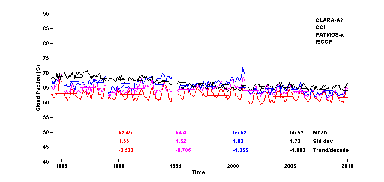
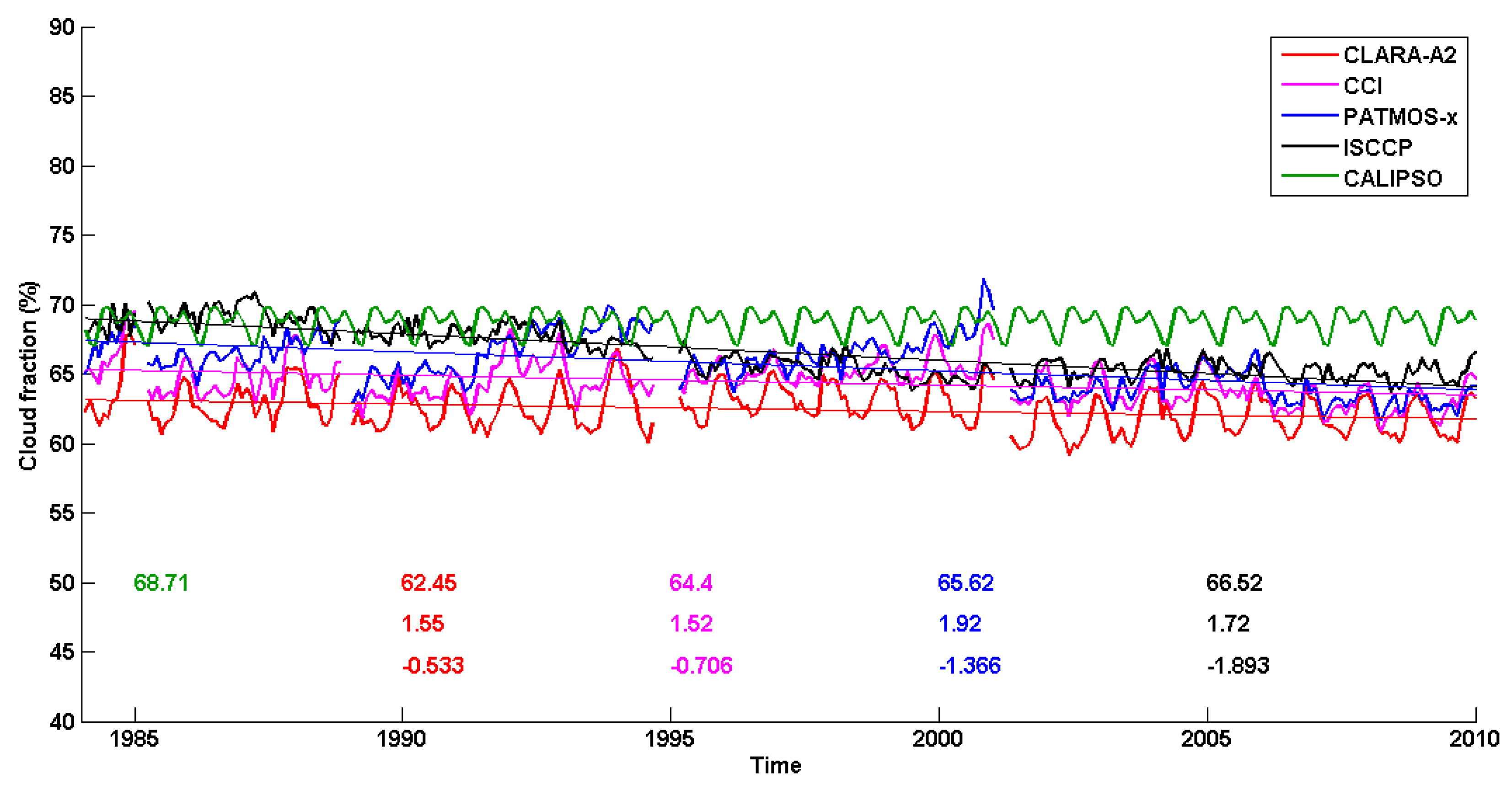
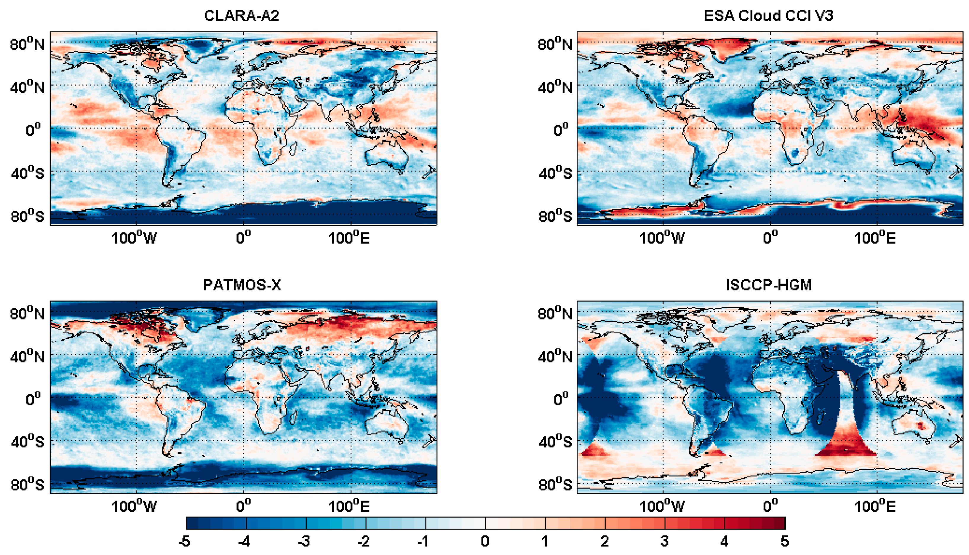
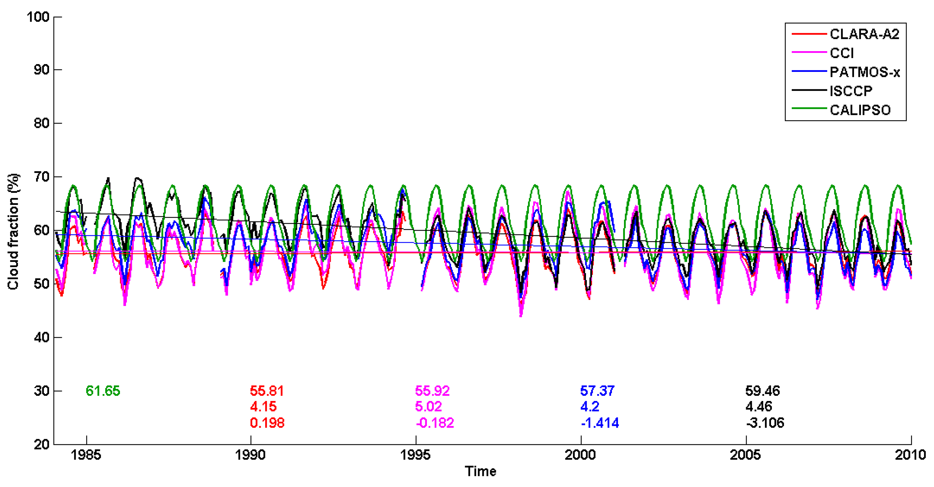
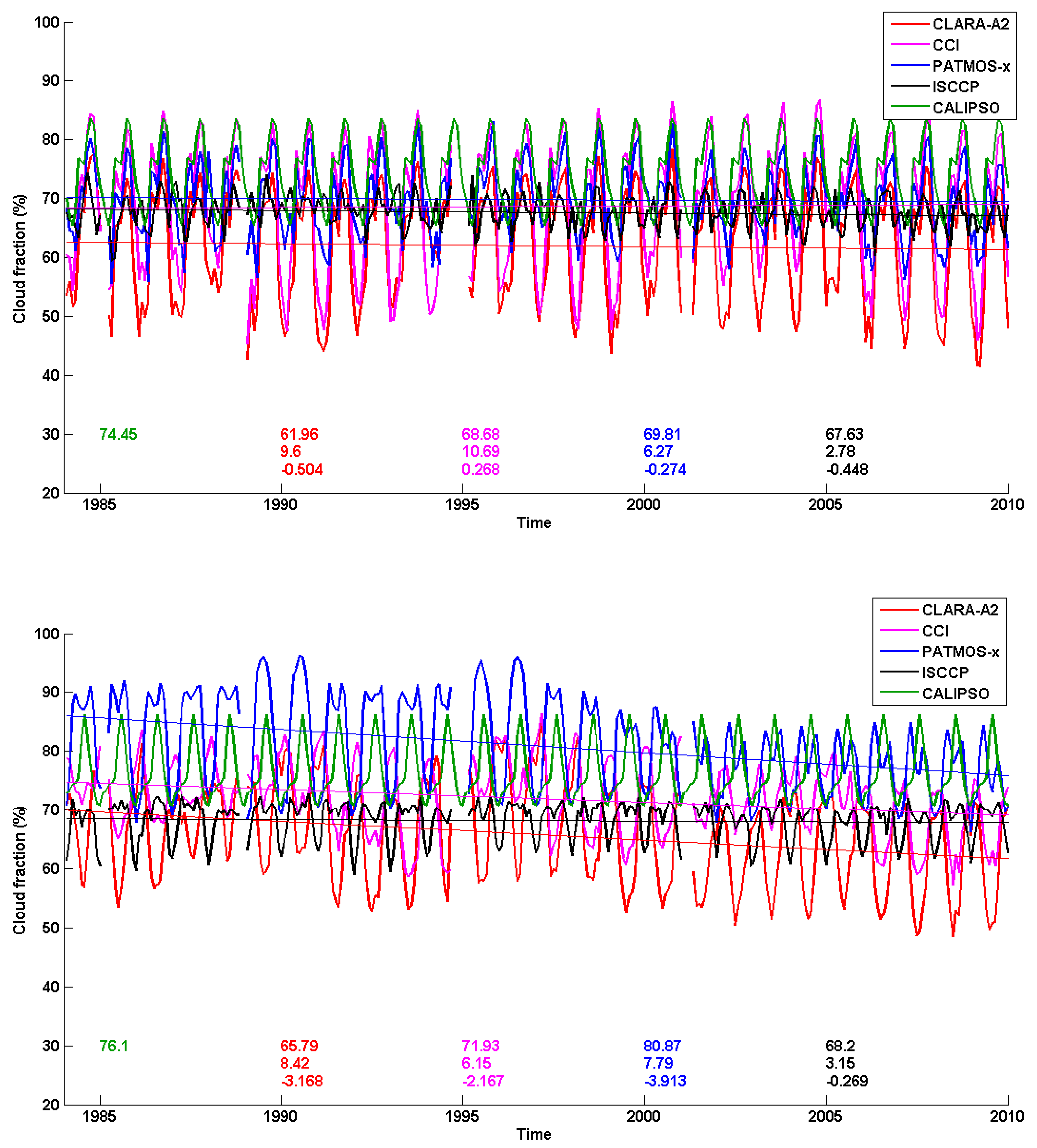
Results for the globally averaged total cloud fraction show that there is in general large agreement between the investigated CDRs, especially from 1995 and onwards. They also all show a weak decreasing trend in global cloudiness although the magnitude differs among them with ISCCP-HGM showing the largest trend (−1.9% per decade) and CLARA-A2 the smallest trend (−0.5% per decade). Despite the overall good agreement, there are interesting differences between the three purely AVHRR-based methods concerning how to deal with orbital drift effects. PATMOS-x shows generally increasing cloud amounts with increasing orbital drift while the other two methods show no or only small changes in cloud amounts. We suggest that these differences are caused by method differences in how to handle the resulting changes in illumination and surface temperature conditions rather than being linked to effects caused by the diurnal cycle in cloudiness which should otherwise have affected all methods in the same way.

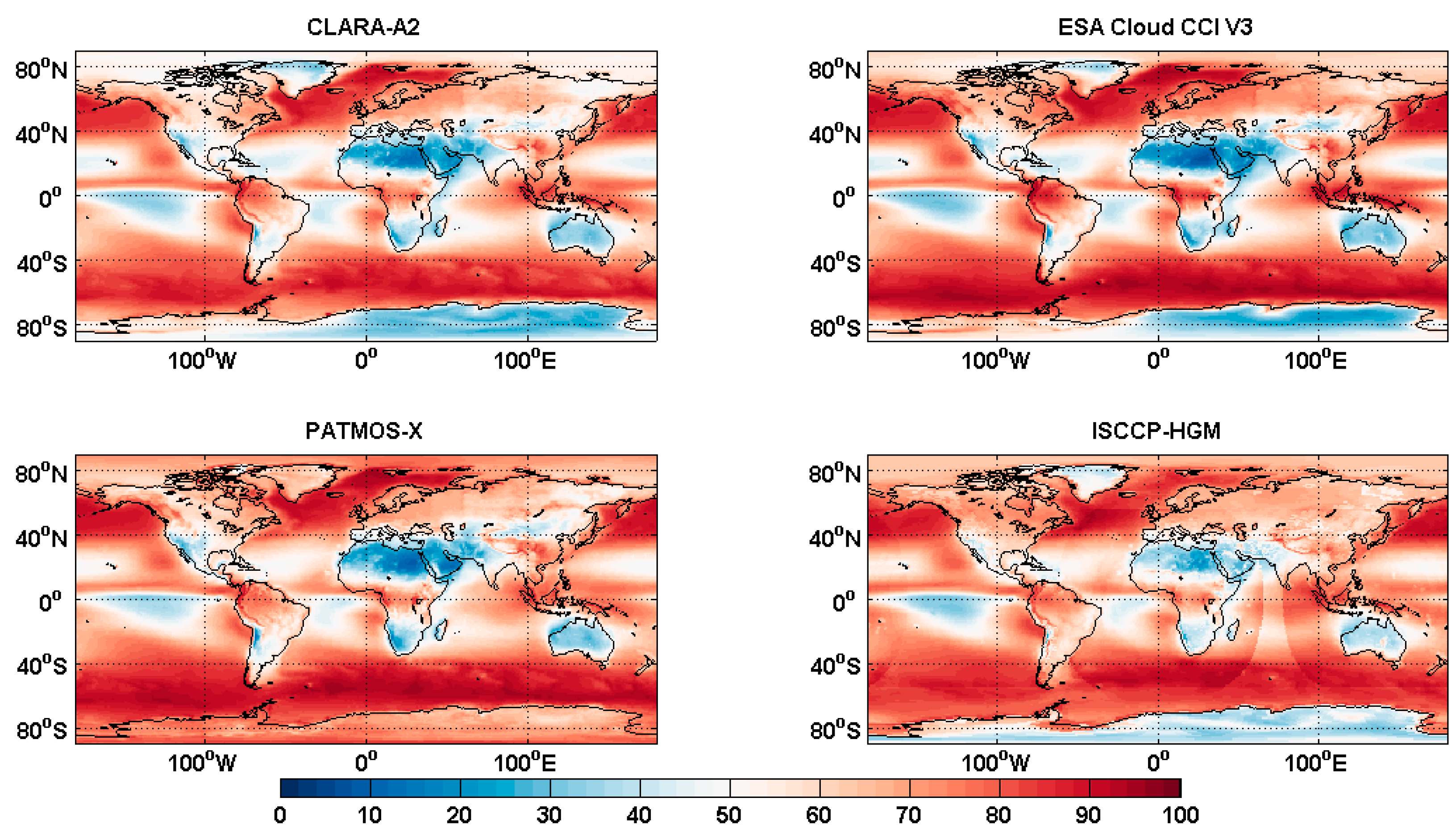
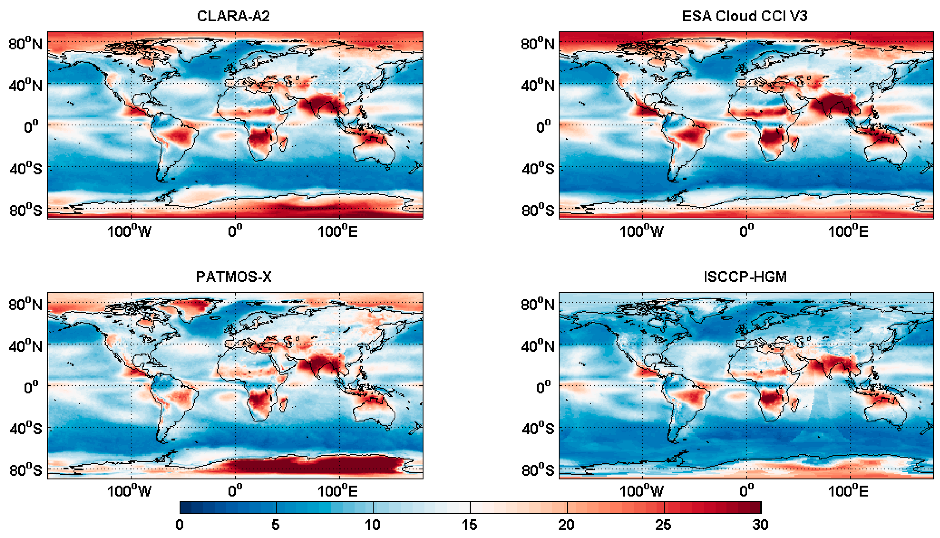
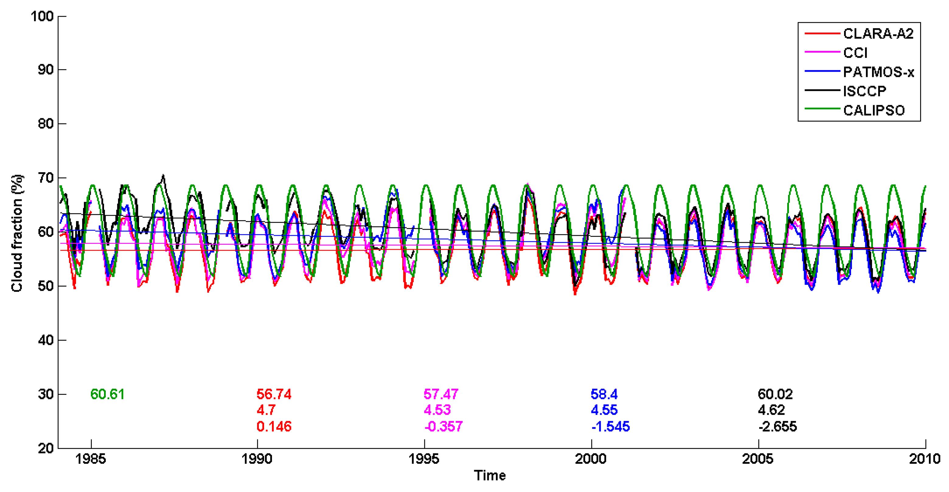
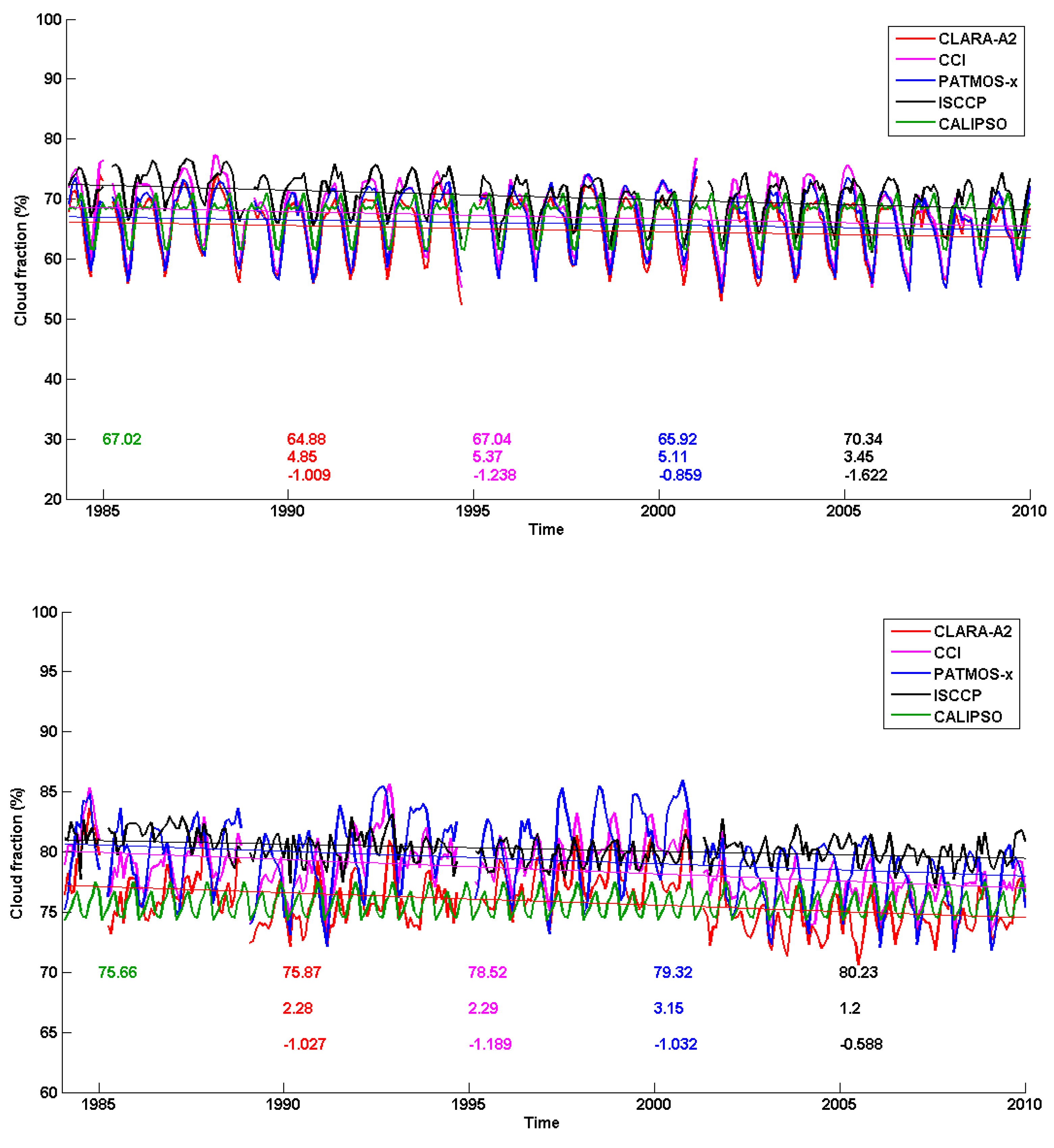
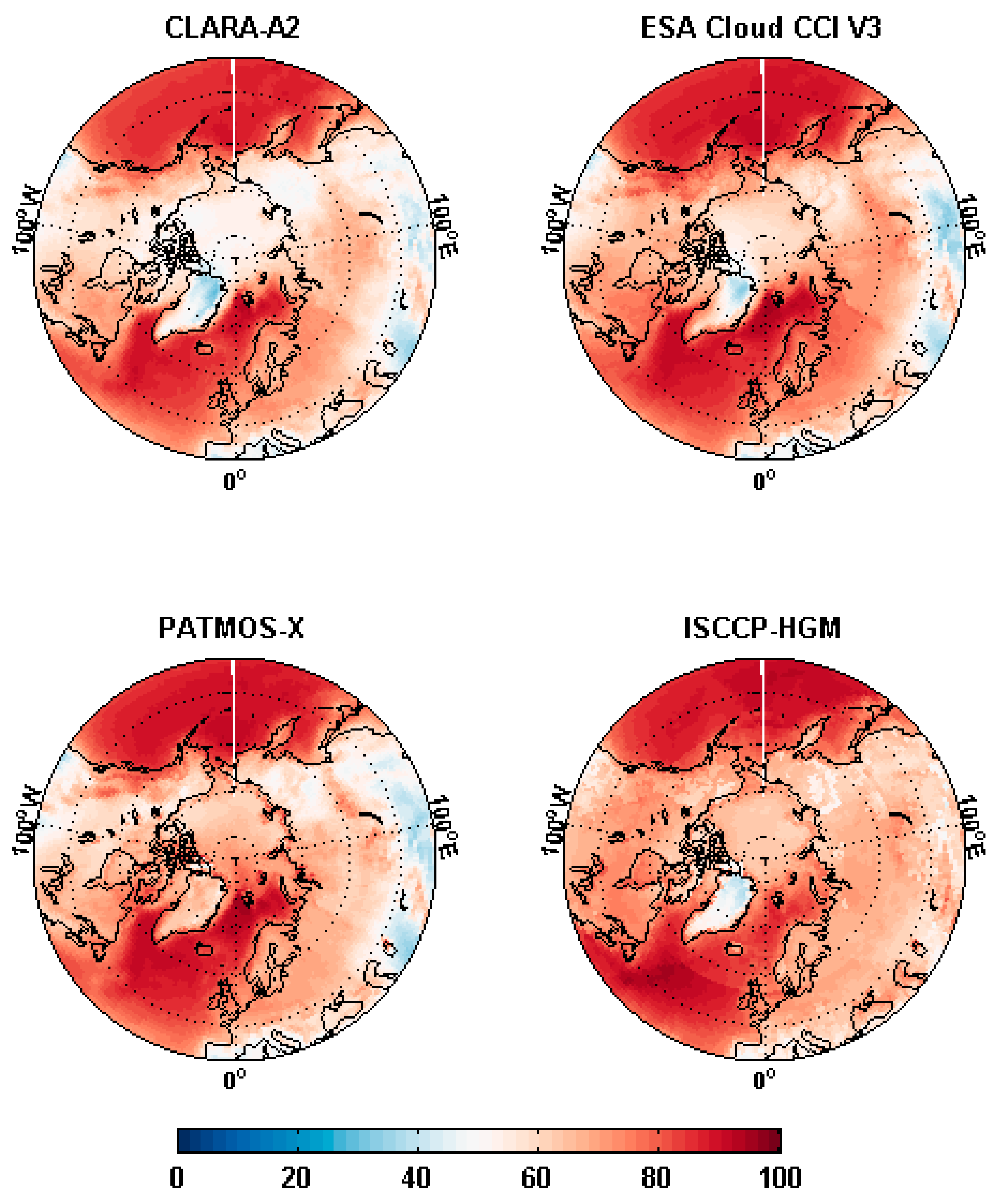
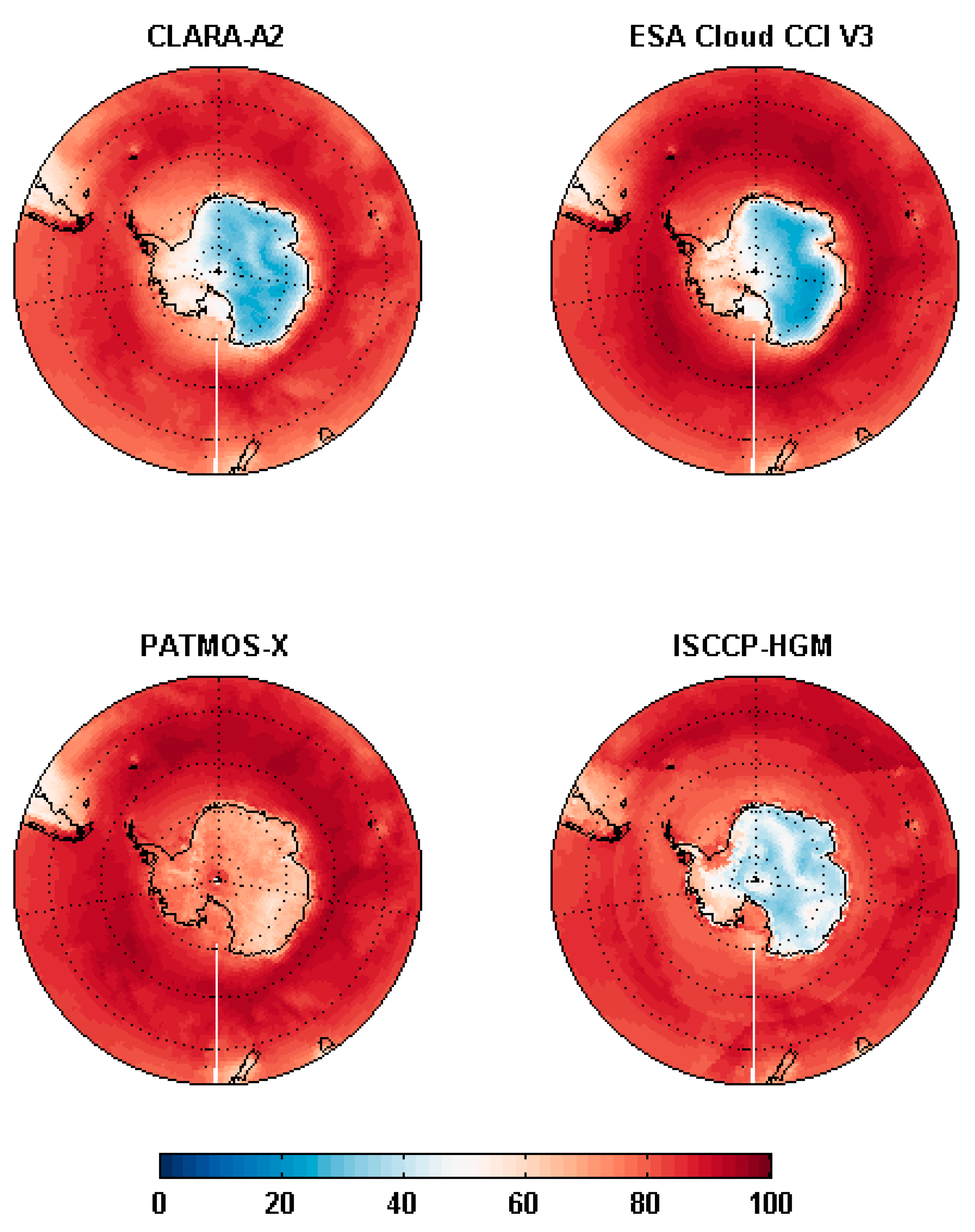
The agreement is most pronounced in the tropical region and in the northern mid-latitude region. Remarkable differences are seen over the southern mid-latitude region and over the polar regions. All CDRs show larger cloud fractions than the CALIPSO-CALIOP reference over the southern mid-latitude region which at first sight could appear surprising considering the higher sensitivity of the CALIOP measurement. However, in areas with high cloud amounts (like the southern mid-latitude region) the viewing geometry differences between the nadir looking CALIOP sensor and passive imagery (operating over a wide range of viewing angles) becomes more evident than over other areas. Higher viewing angles lead to higher interpreted cloud amounts for the passive instruments. The polar regions continue to be challenging for all CDRs and cloud detection results vary substantially here. Polar summer and early autumn cloud amounts appear to be reasonably well depicted by most CDRs over the North Pole region when comparing to the CALIPSO-CALIOP reference. However, ISCCP-HGM cloud amounts are clearly too low. Polar winter results differ remarkably between the south and north poles. Over the North Pole all methods underestimate cloud amounts except ISCCP-HGM (producing almost the same cloud amounts over the year) but over the South Pole the pure AVHRR-based methods show diverging results. PATMOS-x shows here a peak in cloudiness in the polar winter while the other two CDRs generally show minimum values. Best agreement with the CALIPSO-CALIOP reference is found for PATMOS-x.

The overall best agreement (seen over all regions) for the total cloud cover with the CALIPSO-CALIOP reference is consequently found for PATMOS-x, mostly because of its good agreement over the poles. However, this conclusion can be questioned after noting that PATMOS-x cloud amounts are often equal or even exceeding the CALIPSO-CALIOP reference values if excluding the tropical region. It is also remarkable to find so much better results for PATMOS-x compared to the others in the polar winter season over Antarctica where traditionally most methods based on passive imagery have always had large difficulties in separating clouds from the cold surface. Further studies are needed here to confirm that this is based on a real ability to separate the cloudy and cloud-free signature or whether it is a sign of having fitted the data too tight to the overall cloud climatology as provided by the training dataset from CALIPSO-CALIOP.

A detailed inter-comparison of simultaneous cloud observations from ESA Cloud CCI V3 and CALIPSO-CALIOP revealed very good agreement (hit rate of 82.9% and Kuipers skill score of 0.699) between the two which is clearly better than what has been reported in previous similar studies. It shows that it is possible to achieve cloud masking results from ANN-based methods which are superior to results from more traditional methods. Considering the rapid development of machine learning methods, this finding could largely influence future strategies for compiling satellite-based CDRs.

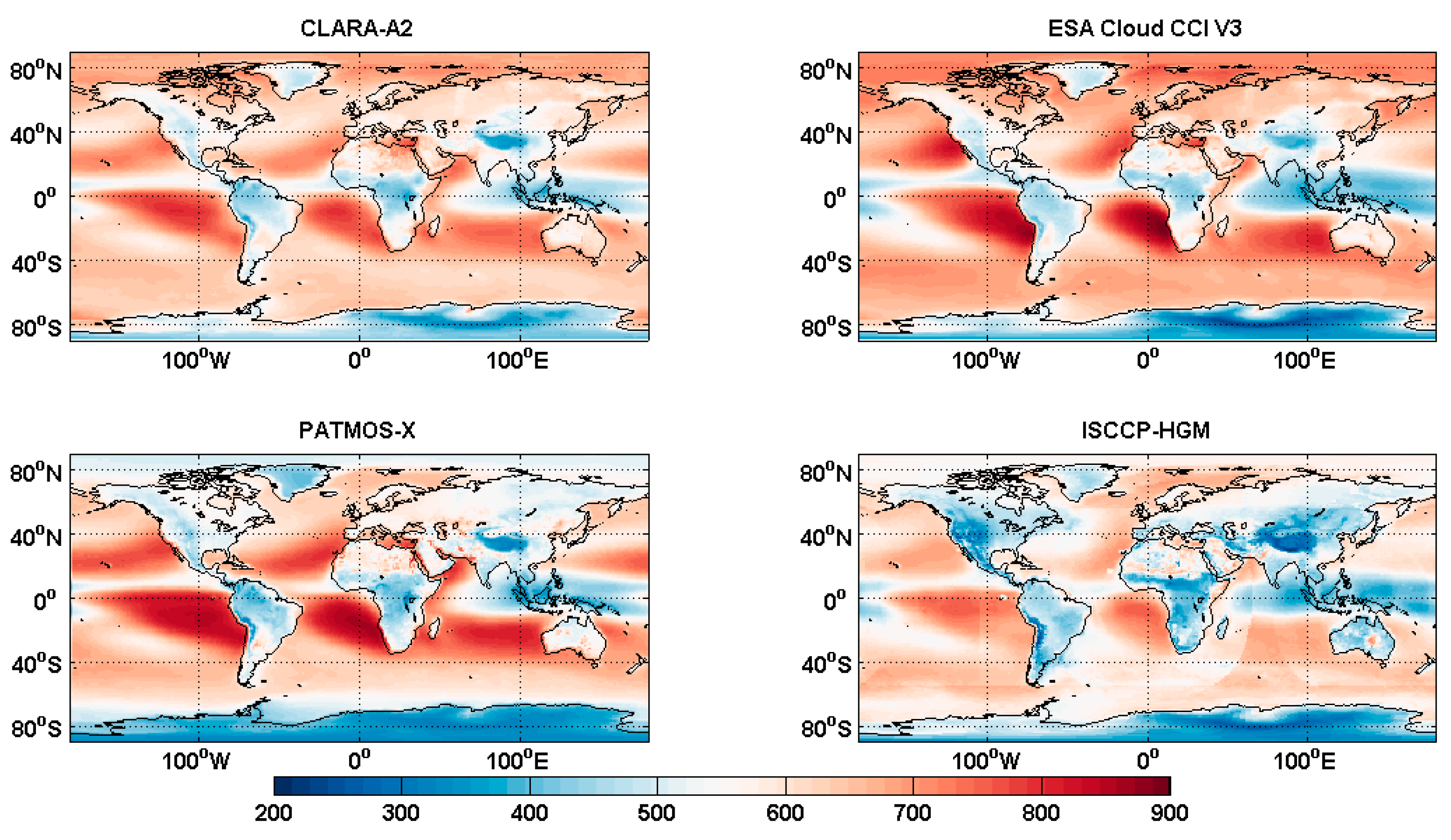
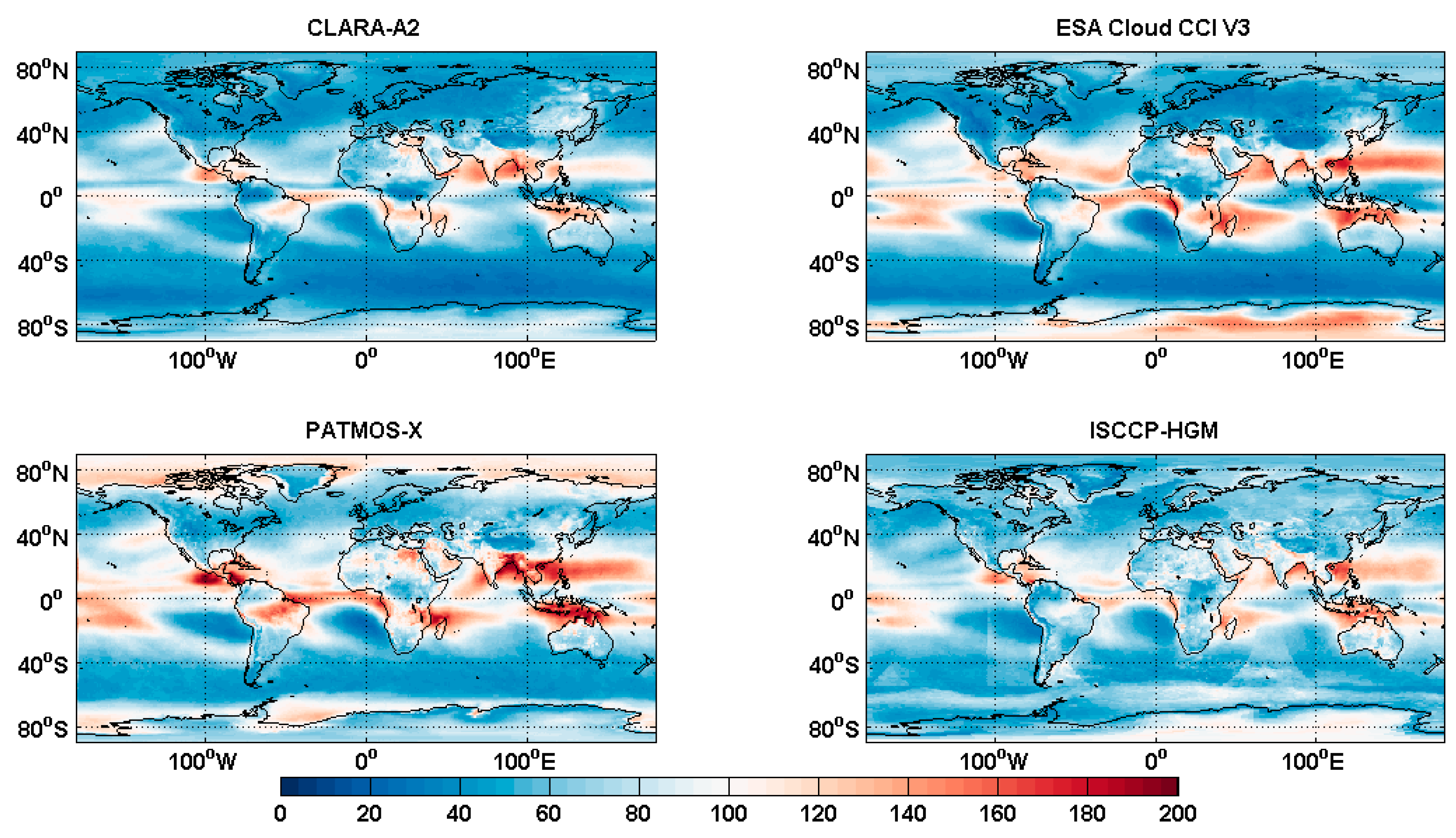
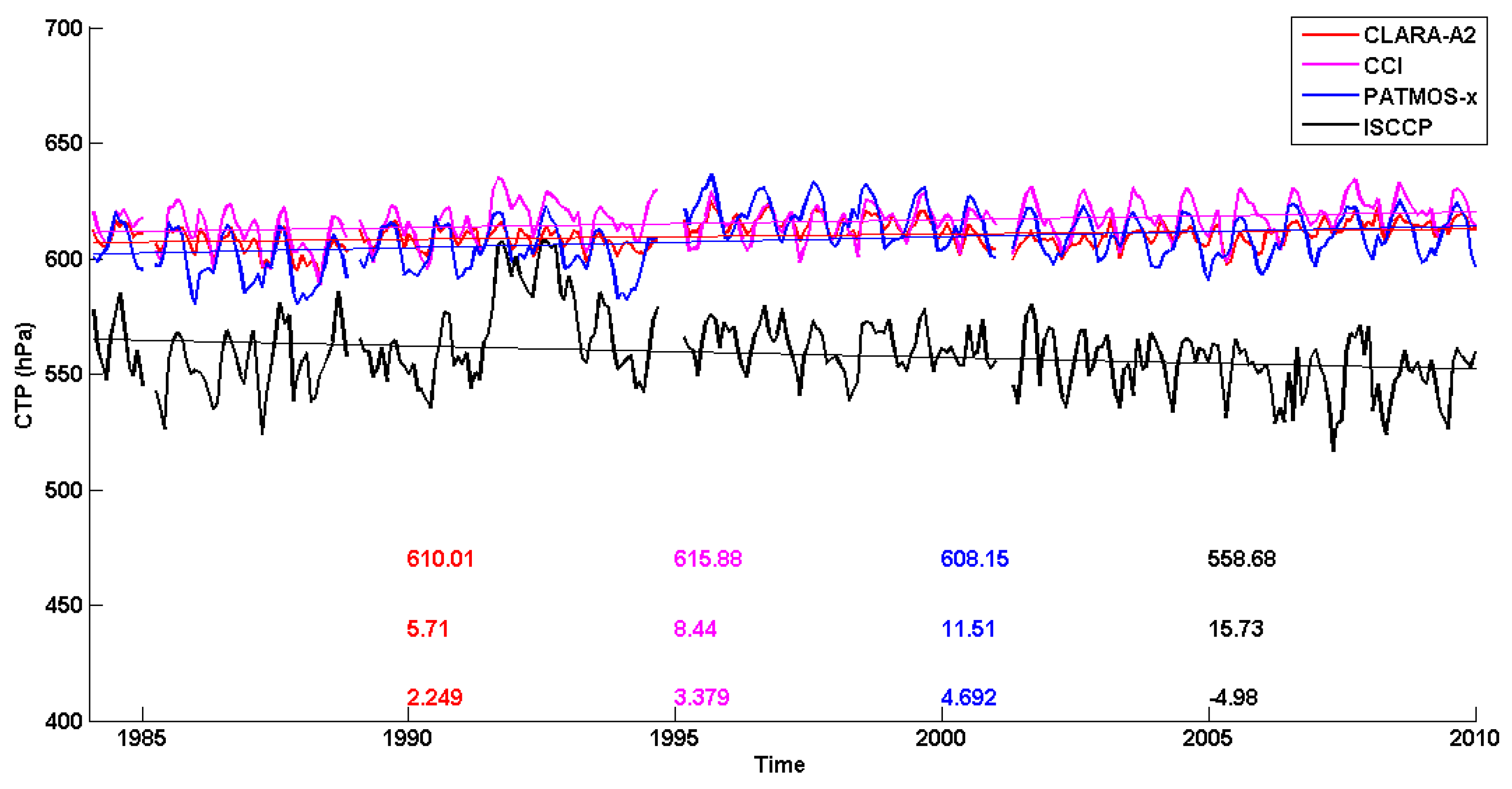
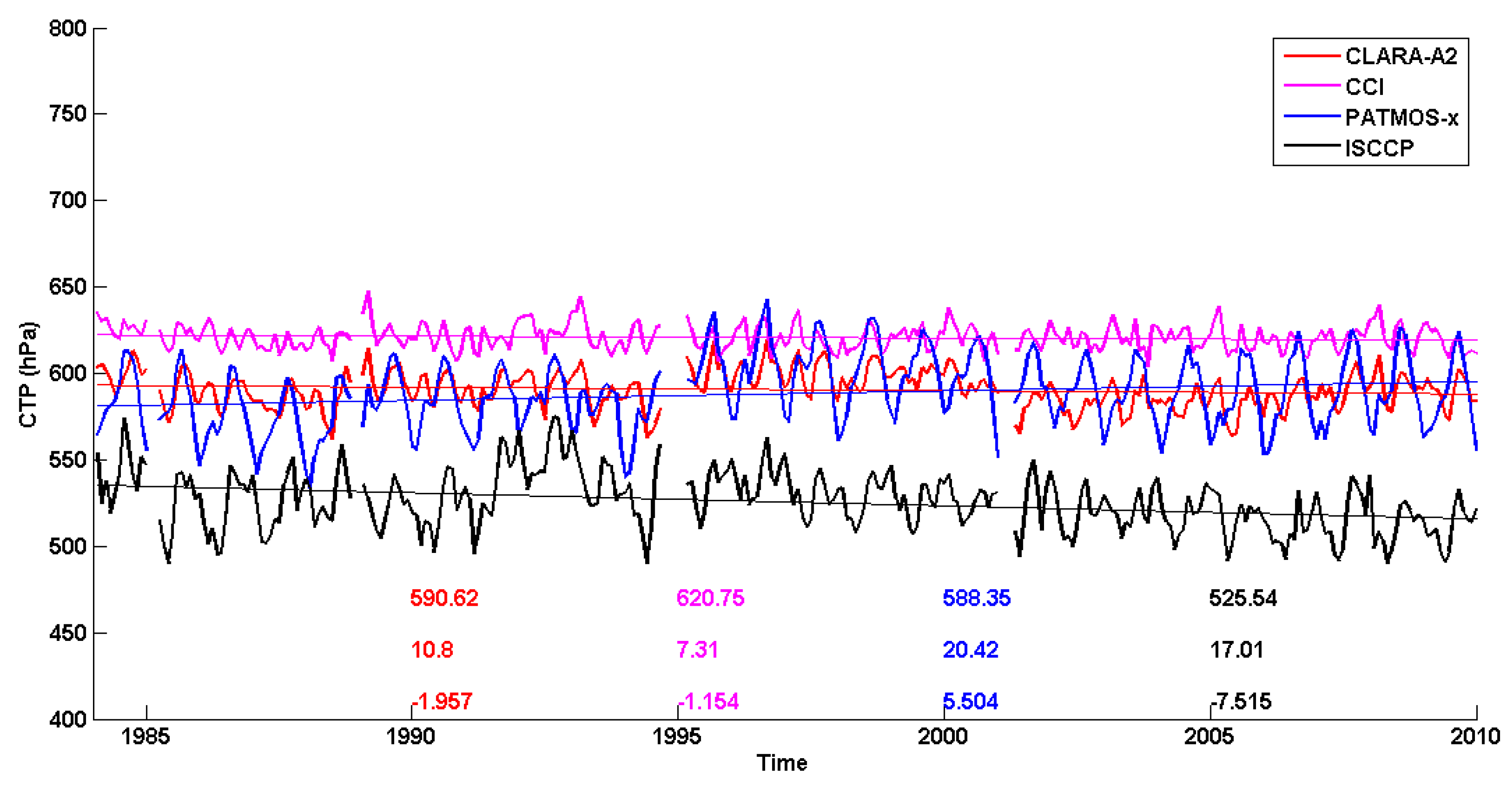
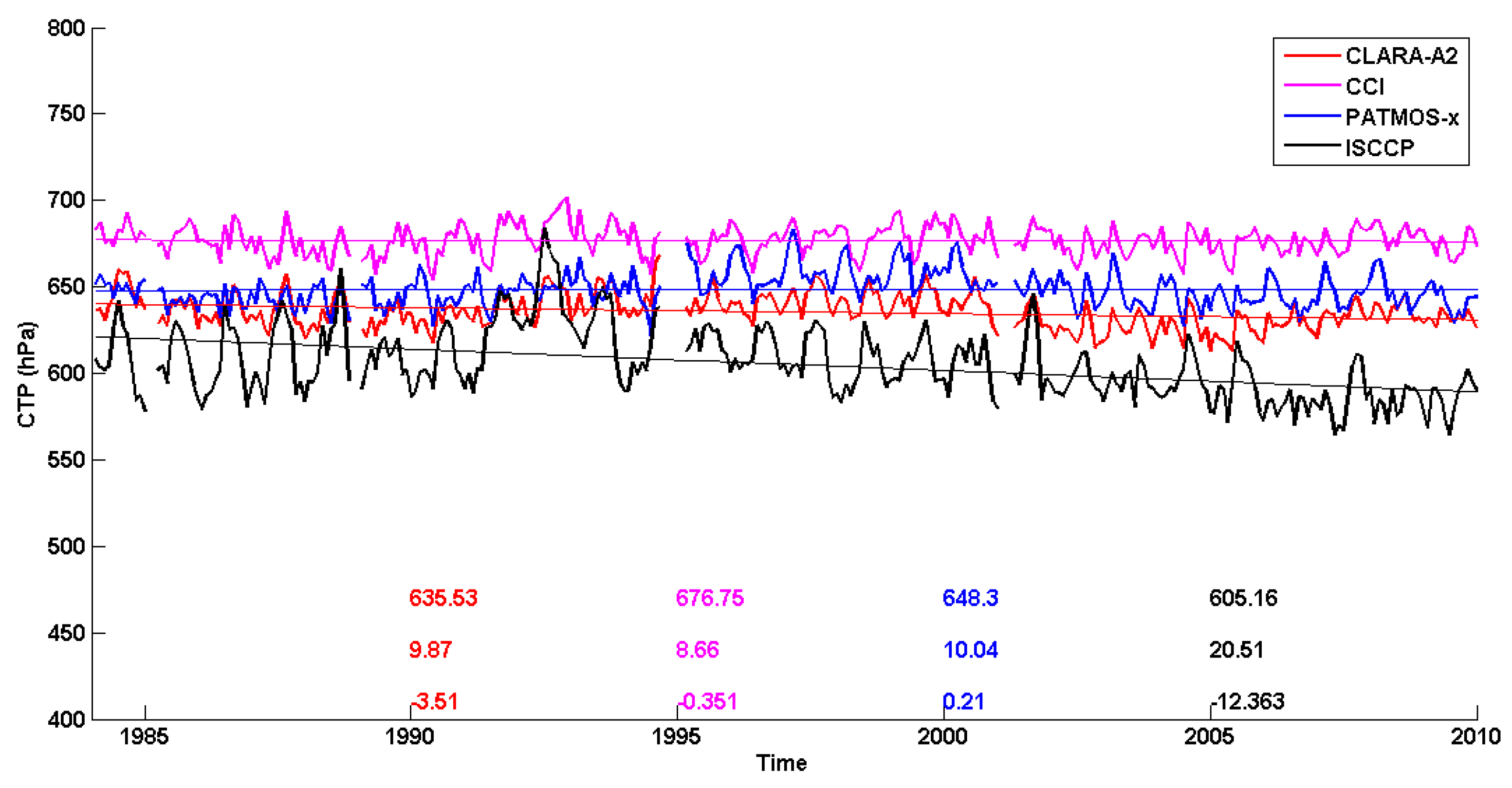
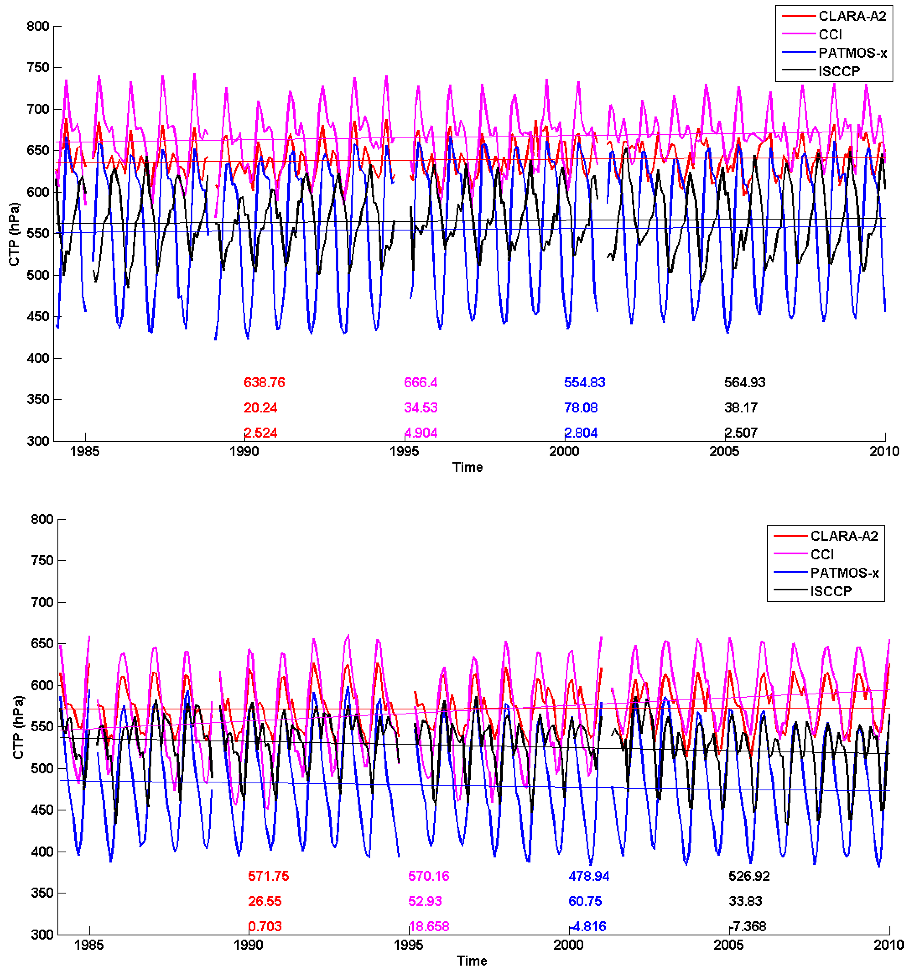
ISCCP-HGM cloud amounts agree reasonable well with the other CDRs over all areas except over the polar regions where the existing seasonal variability is not captured at all. The inter-comparison of cloud top pressure results revealed fundamentally different results for the exclusively AVHRR-based CDRs and the combined geostationary and polar CDR in ISCCP-HGM. The latter showed overall about 60 hPa lower global mean cloud top pressures than the others. In addition, ISCCP-HGM shows a negative trend of 5 hPa per decade over the period as opposed to the others showing positive trends ranging from 2–5 hPa. Further studies are needed to understand this different behavior of cloud top retrievals between the CDRs. Otherwise, it seems that ISCCP-HGM results do not deviate much from the previous version of the ISCCP CDR.

References

1. Stocker, T.F.; Qin, D.; Plattner, G.-K.; Alexander, L.V.; Allen, S.K.; Bindoff, N.L.; Bréon, F.-M.; Church, J.A.; Cubasch, U.; Emori, S.; et al. Technical Summary. In Climate Change 2013: The Physical Science Basis. Contribution of Working Group I to the Fifth Assessment Report of the Intergovernmental Panel on Climate Change; Stocker, T.F., Qin, D., Plattner, G.-K., Tignor, M., Allen, S.K., Boschung, J., Nauels, A., Xia, Y., Bex, V., Midgley, P.M., Eds.; Cambridge University Press: Cambridge, UK; New York, NY, USA, 2013. [Google Scholar]
2. Bony, S.; Stevens, B.; Frierson, D.M.W.; Jakob, C.; Kageyama, M.; Pincus, R.; Shepherd, T.G.; Sherwood, S.C.; Siebesma, A.P.; Sobel, A.H.; et al. Clouds, circulation and climate sensitivity. Nat. Geosci. 2015, 8, 261–268. [Google Scholar] [CrossRef]
3. Vial, J.; Dufresne, J.-L.; Bony, S. On the interpretation of inter-model spread in CMIP5 climate sensitivity estimates. Clim. Dyn. 2013, 41, 3339–3362. [Google Scholar] [CrossRef]
4. Cronin, T.W.; Wing, A.A. Clouds, circulation, and climate sensitivity in a radiative-convective equilibrium channel model. J. Adv. Model. Earth Syst. 2017, 9, 2883–2905. [Google Scholar] [CrossRef]
5. Webb, M.J.; Lambert, F.H.; Gregory, J.M. Origins of differences in climate sensitivity, forcing and feedback in climate models. Clim. Dyn. 2013, 40, 677–707. [Google Scholar] [CrossRef]
6. Huh, O.K.; DiRosa, D. Analysis and interpretation of TIROS-N AVHRR infrared imagery, western Gulf of Mexico. Rem. Sens. Environ. 1981, 11, 371–383. [Google Scholar] [CrossRef]
7. OSCAR—List of All Satellites. Available online: http://www.wmo-sat.info/oscar/satellites (accessed on 27 September 2018).
8. Schiffer, R.A.; Rossow, W.B. The International Satellite Cloud Climatology Project (ISCCP): The first project of the World Climate Research Programme. Bull. Am. Meteorol. Soc. 1983, 64, 779–784. [Google Scholar] [CrossRef]
9. Rossow, W.B.; Schiffer, R.A. ISCCP cloud data products. Bull. Am. Meteorol. Soc. 1991, 72, 2–20. [Google Scholar] [CrossRef]
10. Rossow, W.B.; Schiffer, R.A. Advances in understanding clouds from ISCCP. Bull. Am. Meteorol. Soc. 1999, 80, 2261–2287. [Google Scholar] [CrossRef]
11. Tselioudis, G.; Rossow, W.B.; Zhang, Y.; Konsta, D. Global Weather States and Their Properties from Passive and Active Satellite Cloud Retrievals. J. Clim. 2013, 26, 7734–7746. [Google Scholar] [CrossRef]
12. Bodas-Salcedo, A.; Webb, M.J.; Bony, S.; Chepfer, H.; Dufresne, J.-L.; Klein, S.A.; Zhang, Y.; Marchand, R.; Haynes, J.M.; Pincus, R.; et al. COSP: Satellite simulation software for model assessment. Bull. Am. Meteorol. Soc. 2011, 92, 1023–1043. [Google Scholar] [CrossRef] [Green Version]
13. Klein, S.A.; Zhang, Y.; Zelinka, M.D.; Pincus, R.; Boyle, J.; Gleckler, P.J. Are climate model simulations of clouds improving? J. Geophys. Res. Atmos. 2013, 118, 1329–1342. [Google Scholar] [CrossRef]
14. Norris, J.R.; Evan, A.T. Empirical Removal of Artifacts from the ISCCP and PATMOS-x Satellite Cloud Records. J. Atmos. Ocean. Technol. 2015, 32, 691–702. [Google Scholar] [CrossRef]
15. Inoue, T. On the temperature and effective emissivity determination of semi-transparent cirrus clouds by bi-spectral measurements in the 10 μm window region. J. Meteorol. Soc. Jpn. 1985, 63, 88–99. [Google Scholar] [CrossRef]
16. Inoue, T. A cloud type classification with NOAA-7 split window measurements. J. Geophys. Res. 1987, 92, 3991–4000. [Google Scholar] [CrossRef]
17. Heidinger, A.K.; Foster, M.J.; Walther, A.; Zhao, Z. The Pathfinder Atmospheres Extended (PATMOS-x) AVHRR climate data set. Bull. Am. Meteorol. Soc. 2014, 95, 909–922. [Google Scholar] [CrossRef]
18. Karlsson, K.-G.; Riihelä, A.; Müller, R.; Meirink, J.F.; Sedlar, J.; Stengel, M.; Lockhoff, M.; Trentmann, J.; Kaspar, F.; Hollmann, R.; et al. CLARA-A1: A cloud, albedo, and radiation dataset from 28 yr of global AVHRR data. Atmos. Chem. Phys. 2013, 13, 5351–5367. [Google Scholar] [CrossRef]
19. Stubenrauch, C.J.; Rossow, W.B.; Kinne, S.; Ackerman, S.; Cesana, G.; Chepfer, H.; Di Girolamo, L.; Getzewich, B.; Guignard, A.; Heidinger, A.; et al. Assessment of global cloud datasets from satellites: Project and Database initiated by the GEWEX Radiation Panel. Bull. Am. Meteorol. Soc. 2013, 23, 1031–1049. [Google Scholar] [CrossRef]
20. Karlsson, K.-G.; Anttila, K.; Trentmann, J.; Stengel, M.; Meirink, J.F.; Devasthale, A.; Hanschmann, T.; Kothe, S.; Jääskeläinen, E.; Sedlar, J.; et al. CLARA-A2: The second edition of the CM SAF cloud and radiation data record from 34 years of global AVHRR data. Atmos. Chem. Phys. 2017, 17, 5809–5828. [Google Scholar] [CrossRef]
21. Karlsson, K.-G.; Håkansson, N. Characterization of AVHRR global cloud detection sensitivity based on CALIPSO-CALIOP cloud optical thickness information: Demonstration of results based on the CM SAF CLARA-A2 climate data record. Atmos. Meas. Tech. 2018, 11, 633–649. [Google Scholar] [CrossRef]
22. Winker, D.M.; Vaughan, M.A.; Omar, A.; Hu, Y.; Powell, K.A. Overview of the CALIPSO mission and CALIOP data processing algorithms. J. Atmos. Ocean. Technol. 2009, 26, 2310–2323. [Google Scholar] [CrossRef]
23. Hollmann, R.; Merchant, C.J.; Saunders, R.; Downy, C.; Buchwitz, M.; Cazenave, A.; Chuvieco, E.; Defourny, P.; de Leeuw, G.; Forsberg, R.; et al. The ESA Climate Change Initiative—Satellite Data Records for Essential Climate Variables. Bull. Am. Meteorol. Soc. 2013, 94, 1541–1552. [Google Scholar] [CrossRef]
24. Stengel, M.; Stapelberg, S.; Sus, O.; Schlundt, C.; Poulsen, C.; Thomas, G.; Christensen, M.; Carbajal Henken, C.; Preusker, R.; Fischer, J.; et al. Cloud property datasets retrieved from AVHRR, MODIS, AATSR and MERIS in the framework of the Cloud_cci project. Earth Syst. Sci. Data 2017, 9, 881–904. [Google Scholar] [CrossRef] [Green Version]
25. Young, A.H.; Knapp, K.R.; Inamdar, A.; Hankins, W.; Rossow, W.B. The International Satellite Cloud Climatology Project H-Series climate data record product. Earth Syst. Sci. Data 2018, 10, 1–11. [Google Scholar] [CrossRef]
26. Chepfer, H.; Bony, S.; Winker, D.M.; Cesana, G.; Dufresne, J.-L.; Minnis, P.; Stubenrauch, C.J.; Zeng, S. The GCM Oriented CALIPSO Cloud Product (CALIPSO-GOCCP). J. Geophys. Res. 2010, 115, D00H16. [Google Scholar] [CrossRef]
27. Baum, B.; Menzel, W.P.; Frey, R.; Tobin, D.; Holz, R.; Ackerman, S. MODIS Cloud Top Property Refinements for Collection 6. J. Appl. Meteorol. Clim. 2012, 51, 1145–1163. [Google Scholar] [CrossRef]
28. Platnick, S.; Meyer, K.; King, M.D.; Wind, G.; Amarasinghe, N.; Marchant, B.; Arnold, G.T.; Zhang, Z.; Hubanks, P.A.; Holz, R.E.; et al. The MODIS cloud optical and microphysical products: Collection 6 updates and examples from Terra and Aqua. IEEE Trans. Geosci. Remote Sens. 2017, 55, 502–525. [Google Scholar] [CrossRef] [PubMed]
29. Sus, O.; Stengel, M.; Stapelberg, S.; McGarragh, G.; Poulsen, C.; Povey, A.C.; Schlundt, C.; Thomas, G.; Christensen, M.; Proud, S.; et al. The Community Cloud retrieval for Climate (CC4CL). Part I: A framework applied to multiple satellite imaging sensors. Atmos. Meas. Tech. 2018, 11, 3373–3396. [Google Scholar] [CrossRef]
30. McGarragh, G.R.; Poulsen, C.A.; Thomas, G.E.; Povey, A.C.; Sus, O.; Stapelberg, S.; Schlundt, C.; Proud, S.; Christensen, M.W.; Stengel, M.; et al. The Community Cloud retrieval for CLimate (CC4CL). Part II: The optimal estimation approach. Atmos. Meas. Tech. 2018, 11, 3397–3431. [Google Scholar] [CrossRef]
31. Rodgers, C.D. Retrieval of Atmospheric Temperature and Composition From Remote Measurements of Thermal Radiation. Rev. Geophys. Space Phys. 1976, 14, 609–624. [Google Scholar] [CrossRef]
32. Rodgers, C.D. Inverse Methods for Atmospheric Sounding: Theory and Practice; World Scientific Publishing Co.: River Edge, NJ, USA, 2000. [Google Scholar]
33. Stengel, M.; Stapelberg, S.; Sus, O.; Finkensieper, S.; Würzler, B.; Philipp, D.; Poulsen, C.; Christensen, M.; McGarragh, G.R. Cloud cci AVHRR version 3.0 datasets: 35 yr climatologies of global cloud and radiation properties. Earth Syst. Sci. Data 2018. in preparation. [Google Scholar]
34. Jacobowitz, H.; Stowe, L.L.; Ohring, G.; Heidinger, A.; Knapp, K.; Nalli, N.R. The Advanced Very High Resolution Radiometer Pathfinder Atmosphere (PATMOS) climate dataset: A resource for climate research. Bull. Am. Meteorol. Soc. 2003, 84, 785–793. [Google Scholar] [CrossRef]
35. Heidinger, A.K.; Evan, A.T.; Foster, M.J.; Walther, A. A naive Bayesian cloud-detection scheme derived from CALIPSO and applied within PATMOS-x. J. Appl. Meteorol. Clim. 2012, 51, 1129–1144. [Google Scholar] [CrossRef]
36. Heidinger, A.K.; Straka, W.C.; Molling, C.C.; Sullivan, J.T.; Wu, X.Q. Deriving an inter-sensor consistent calibration for the AVHRR solar reflectance data record. Int. J. Remote Sens. 2010, 31, 6493–6517. [Google Scholar] [CrossRef]
37. Norris, J.R.; Allen, R.J.; Evan, A.T.; Zelinka, M.D.; O’Dell, C.W.; Klein, S.A. Evidence for climate change in the satellite cloud record. Nature 2016, 536, 72–75. [Google Scholar] [CrossRef] [PubMed]
38. Evan, A.T.; Heidinger, A.K.; Vimont, D.J. Arguments against a physical long-term trend in global ISCCP cloud amounts. Geoph. Res. Lett. 2007, 34. [Google Scholar] [CrossRef] [Green Version]
39. Klein, S.A.; Hartmann, D.L. The seasonal cycle of low stratiform clouds. J. Clim. 1993, 6, 1587–1606. [Google Scholar] [CrossRef]
40. Hines, K.M.; Bromwich, D.H. Simulation of Late Summer Arctic Clouds during ASCOS with Polar WRF. Mon. Weather Rev. 2017, 145, 521–541. [Google Scholar] [CrossRef]
41. Kay, J.E.; L’Ecuyer, T. Observational constraints on Arctic Ocean clouds and radiative fluxes during the early 21st century. J. Geophys. Res. 2013, 118, 7219–7236. [Google Scholar] [CrossRef] [Green Version]
42. Adhikari, L.; Wang, Z.; Deng, M. Seasonal variations of Antarctic clouds observed by Cloudsat and CALIPSO satellites. J. Geophys. Res. 2012, 117. [Google Scholar] [CrossRef]
43. Del Genio, A.D.; Wolf, A.D.; Yao, M.-S. Evaluation of regional cloud feedbacks using single column models. J. Geophys. Res. 2005, 110, D15S13. [Google Scholar] [CrossRef]
44. Schmidt, G.A.; Ruedy, R.; Hansen, J.E.; Aleinov, I.; Bell, N.; Bauer, M.; Bauer, S.; Cairns, B.; Canuto, V.; Cheng, Y.; et al. Present-Day Atmospheric Simulations Using GISS ModelE: Comparison to In Situ, Satellite, and Reanalysis Data. J. Clim. 2006, 19, 153–192. [Google Scholar] [CrossRef]
45. Heidinger, A.; Foster, M.; Botambekov, D.; Hiley, M.; Walther, A.; Li, Y. Using the NASA EOS A-Train to Probe the Performance of the NOAA PATMOS-x Cloud Fraction CDR. Remote Sens. 2016, 8, 511–528. [Google Scholar] [CrossRef]
Figure 1. Climatological mean total cloud fraction averaged over 26-year period (1984–2009) in four CDRs.
Remotesensing 10 01567 g001
Figure 2. Standard deviation in total cloud fraction over the same 26-year time period.
Remotesensing 10 01567 g002
Figure 3. Time series showing global total cloud fraction from various CDRs. The numbers show mean, standard deviation, and trend per decade for each CDR.
Remotesensing 10 01567 g003
Figure 4. Spatial distribution of trends in total cloud fraction (% per decade) for the investigated CDRs.
Remotesensing 10 01567 g004
Figure 5. Same as in Figure 3, but for the northern tropical (top panel) and the southern tropical regions (bottom panel).
Remotesensing 10 01567 g005aRemotesensing 10 01567 g005b
Figure 6. Same as in Figure 3, but for the northern mid-latitude (top panel) and the southern mid-latitude regions (bottom panel).
Remotesensing 10 01567 g006
Figure 7. Same as in Figure 3, but for the North Pole (top panel) and the South Pole (bottom panel).
Remotesensing 10 01567 g007
Figure 8. Climatological mean total cloud fraction from various CDRs over the Arctic.
Remotesensing 10 01567 g008
Figure 9. Climatological mean total cloud fraction from various CDRs over the Antarctic.
Remotesensing 10 01567 g009
Figure 10. Climatological mean cloud top pressure (hPa) averaged over 26-year period (1984–2009) in four CDRs.
Remotesensing 10 01567 g010
Figure 11. Standard deviation in cloud top pressures (hPa) over the same 26-year time period.
Remotesensing 10 01567 g011
Figure 12. Inter-comparison of globally averaged cloud top pressures.
Remotesensing 10 01567 g012
Figure 13. Spatial distribution of trends in cloud top pressure (hPa per decade) for the investigated CDRs.
Remotesensing 10 01567 g013
Figure 14. Time series of cloud top pressures averaged over the northern tropical (top panel) and the southern tropical regions (bottom panel).
Remotesensing 10 01567 g014
Figure 15. Same as in Figure 14, but for the northern mid-latitude (top panel) and the southern mid-latitude (bottom panel) regions.
Remotesensing 10 01567 g015aRemotesensing 10 01567 g015b
Figure 16. Same as in Figure 12, but for the North Pole (top panel) and the South Pole (bottom panel).
Remotesensing 10 01567 g016
Figure 17. Global map of cloud detection sensitivity (defined in text) for the ESA Cloud CCI V3 cloud mask based on comparisons with CALIPSO-CALIOP in the period 2007–2015. Specific color map features are explained in text.
Remotesensing 10 01567 g017