Article

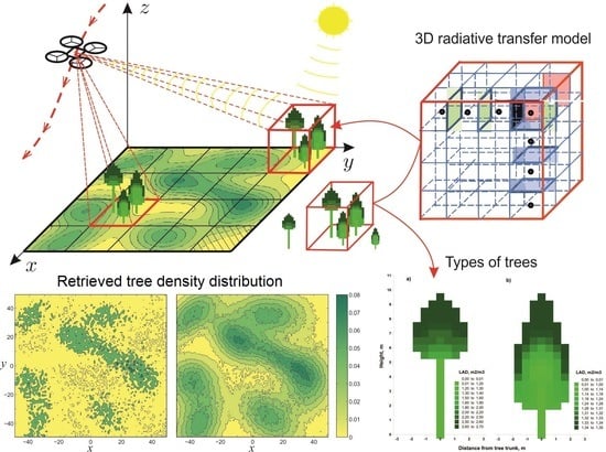
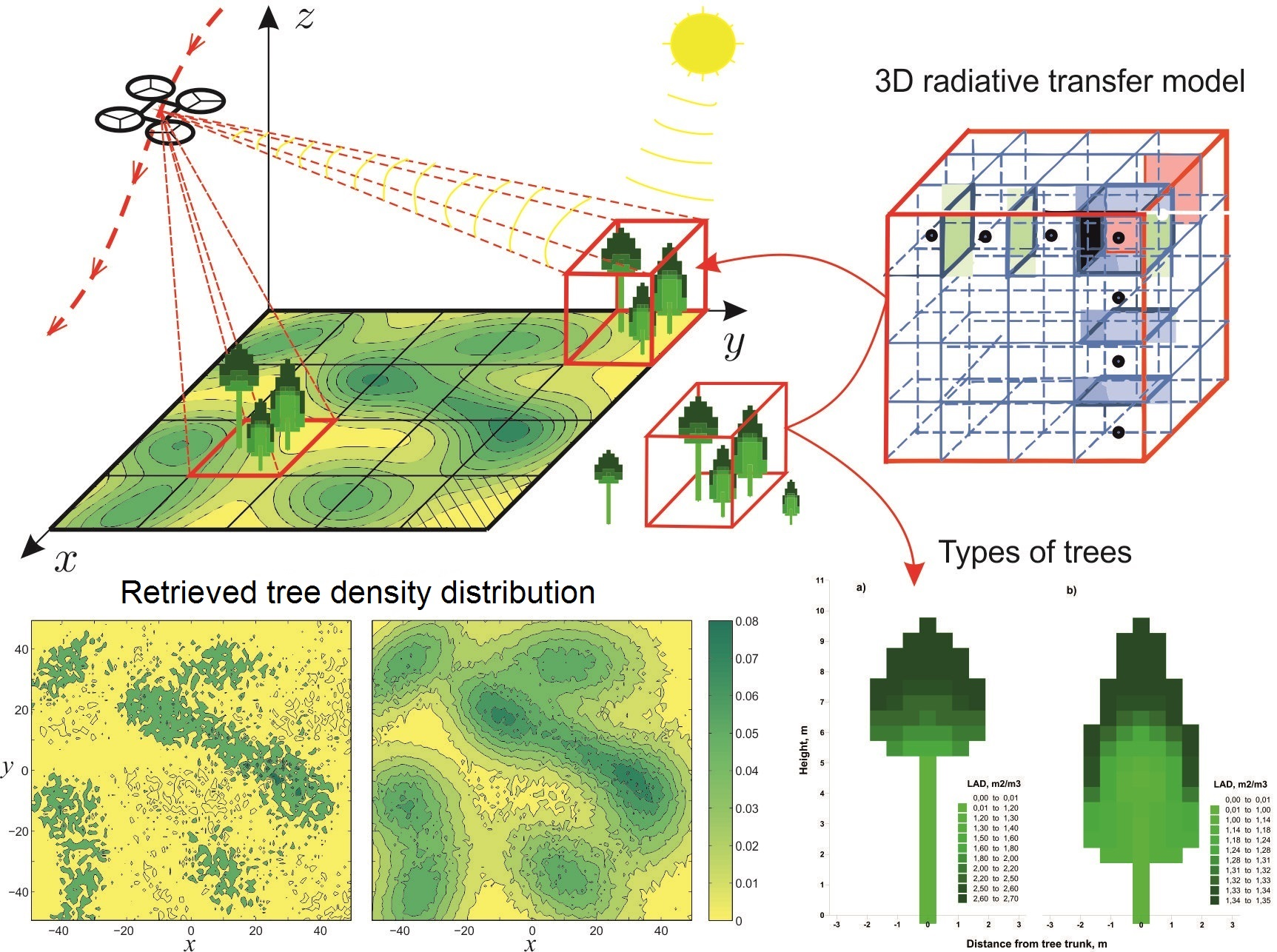
Application of a Three-Dimensional Radiative Transfer Model to Retrieve the Species Composition of a Mixed Forest Stand from Canopy Reflected Radiation

by
Natalia Levashova
1,*,
Dmitry Lukyanenko
1,
Yulia Mukhartova
1 and
Alexander Olchev
2,3
1
Department of Mathematics, Faculty of Physics, Lomonosov Moscow State University, Moscow 119991, Russia
2
Department of Meteorology and Climatology, Faculty of Geography, Lomonosov Moscow State University, Moscow 119991, Russia
3
Laboratory of Biogeocenology, A.N.Severtsov Institute of Ecology and Evolution, Russian Academy of Science, Moscow 119071, Russia
*
Author to whom correspondence should be addressed.
Remote Sens. 2018, 10(10), 1661; https://0-doi-org.brum.beds.ac.uk/10.3390/rs10101661
Submission received: 31 July 2018 / Revised: 12 October 2018 / Accepted: 16 October 2018 / Published: 20 October 2018
(This article belongs to the Special Issue Radiative Transfer Modelling and Applications in Remote Sensing)

Abstract

:
The paper introduces a three-dimensional model to derive the spatial patterns of photosynthetically active radiation (PAR) reflected and absorbed by a non-uniform forest canopy with a multi-species structure, as well as a model algorithm application to retrieve forest canopy composition from reflected PAR measured along some trajectory above the forest stand. This radiative transfer model is based on steady-state transport equations, initially suggested by Ross, and considers the radiative transfer as a function of the structure of individual trees and forest canopy, optical properties of photosynthesizing and non-photosynthesizing parts of the different tree species, soil reflection, and the ratio of incoming direct and diffuse solar radiation. Numerical experiments showed that reflected solar radiation of a typical mixed forest stand consisting of coniferous and deciduous tree species was strongly governed by canopy structure, soil properties and sun elevation. The suggested algorithm based on the developed model allows for retrieving the proportion of different tree species in a mixed forest stand from measured canopy reflection coefficients. The method accuracy strictly depends on the number of points for canopy reflection measurements.

Graphical Abstract

1. Introduction

Solar radiation is both a direct and indirect driver for most biophysical and biochemical processes occurring in plant ecosystems. It influences canopy microclimate as well as CO2 and H2O exchange processes between plants and the atmosphere [1,2], thereby affecting not only the function and growth of the plant community, but also the concentration of greenhouse gases in the atmosphere and consequently, Earth’s climate system [3,4]. Plant canopy reflection and absorption of solar radiation are determined by factors including the structure of vegetation cover, the optical properties of photosynthesizing and non-photosynthesizing parts of plants, surface topography, and soil [1,5]. During recent decades, numerous studies have focused on the theory of solar radiation transfer in a plant canopy [1,6,7,8,9,10], leading to the development and application of mathematical models with different degrees of complexity [11,12,13,14,15,16,17]. Most simple approaches consider the plant canopy as a horizontally uniform turbid medium [13,18,19]. A vertically structured forest canopy can also be divided into many independent sub-layers [10]. The effects of local plant canopy heterogeneity on radiative fluxes in these one-dimensional (1D) approaches are usually ignored. A limited number of input parameters allow these models to be used for a broad spectrum of scientific tasks, including solving direct and inverse problems related to remote sensing [10,15,20].
The effects of local-scale heterogeneity on radiation fluxes at a regional scale are usually assumed to be very small and therefore negligible, but they can be relatively large on an ecosystem level and can cause large biases in the estimation of solar radiation that is reflected, absorbed, and transmitted by a plant canopy [21,22,23]. Complex forest canopy architecture is common along the boundaries between different forest types and this complexity can have significant effects on absorbed and scattered solar radiation. Scientific studies of radiative transfer in such non-uniform plant canopies require more sophisticated and process-based modeling approaches that consider three-dimensional (3D) canopy structure, including the individual structure of different tree species.
There are several detailed reviews of available 3D models for the description of radiative transfer within spatially distributed and non-uniform vegetation [7,10,20]. Many of these works were devoted to the ability of 1D and 3D models to reproduce the mean characteristics of canopy absorption, transmission, and reflection by allowing for mosaic vegetation structure [16,17,24]. Most studies show that 3D models of radiative transfer can be a universal tool to describe the 3D radiation absorption and scattering patterns for a spatially heterogeneous plant canopy. These models are presently used for various ecological and meteorological tasks involving satellite remote sensing (e.g., Landsat, MODIS, DSCOVR EPIC) [15,25,26,27,28,29]. Key parameters that can be determined using such models are total absorbed and reflected solar radiation by a plant canopy and their variance, the fractions of sunlit and shaded leaves, leaf area index of sunlit and shaded leaves, and soil surface reflection/absorption, etc. In considering the reflection of solar radiation from the forest canopy with a multi-specific structure, it is important to also estimate the proportion of various tree species within a forest stand. Such information can be derived from other biophysical properties of the forest canopy and soil, such as leaf area index and the amount of photosynthesizing plant biomass.
In this study we developed and applied a 3D model of radiative transfer in a non-uniform plant canopy to derive the possible influence of multi-specific forest structure on reflected photosynthetically active radiation (PAR). For our numerical experiments, we selected a mixed forest stand consisting of a coniferous and a deciduous tree species with different structure of individual trees, vertical and horizontal biomass distribution, and leaf and shoot optical properties. Mixed deciduous–coniferous forest is a dominant forest type at the southern boundary of the boreal forest and effects of forest structural and optical properties on radiative transfer (reflection, absorption, transmission) have not been sufficiently investigated in the area. Moreover, in this study we proposed and tested an algorithm to retrieve forest canopy composition (proportion of deciduous and coniferous tree species in a forest stand) from the intensity of reflected radiation measured by remote sensing at several points above the forest canopy.

2. Materials and Methods

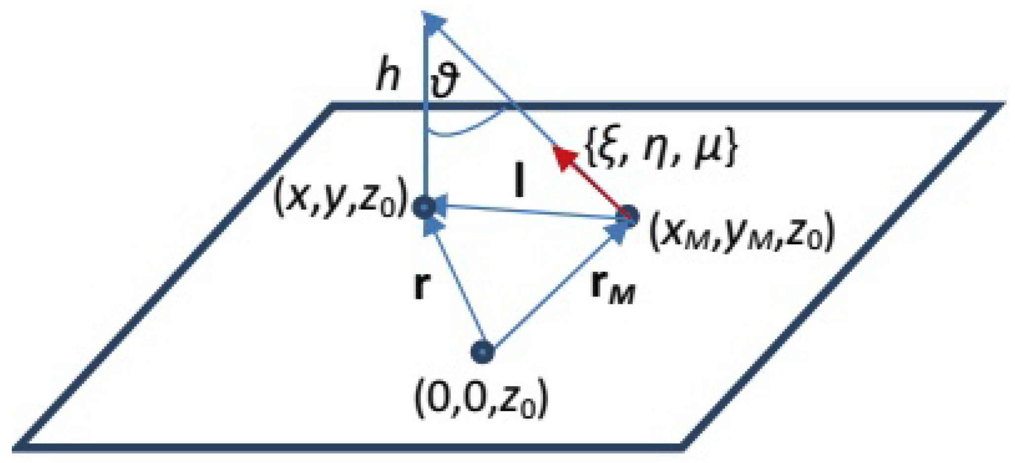
2.1. The 3D Model Description

The 3D radiative transfer model is based on the main equations and assumptions suggested by Ross [1] and further developed and described by Myneni [7,30] and Knyazikhin [22,31]. According to this approach, the function characterizing the radiative field at each spatial point r = { x , y , z } within the vegetation canopy is the radiance I λ ( r , Ω ) , which depends on wavelength λ and is calculated as the sum of the direct and diffuse radiation over all directions defined by vectors Ω = { μ , φ } = { cos φ sin θ , sin φ sin θ , cos θ } , ( φ [ 0 , 2 π ] , θ [ 0 , π ] ).
The spatial pattern of direct radiation within the plant canopy depends on the probability that a sunbeam incident on the upper canopy along the direction Ω0 reaches some point r within the vegetation without being reflected or scattered by vegetation elements [7,30]. The intensity of direct solar radiation within a plant canopy can be expressed as Q 0 , λ ( r ) = T m , λ exp ( 0 l r , Ω 0 σ ( r s Ω 0 , Ω 0 ) d s ) .
Here, T m , λ (W/m2) is the intensity of direct solar radiation at the upper boundary of the vegetation canopy, l r , Ω 0 is the distance between the point r and the upper boundary of vegetation cover along the direction Ω0 to the sun, and σ ( r , Ω ) is the total cross-section of the interaction (scattering and absorption) of solar radiation with vegetation elements (see Appendix A).
The intensity of diffuse radiation at some point r within the vegetation over the direction defined by vector Ω is determined by the equation:
Ω I λ , d ( r , Ω ) + σ ( r , Ω ) I λ , d ( r , Ω ) = 4 π I λ , d ( r , Ω ) σ s λ ( r , Ω Ω ) d Ω + σ s λ ( r , Ω 0 Ω ) Q 0 , λ ( r ) .  
Here σ s λ ( r , Ω Ω ) is the differential cross-section for the scattering of the sun rays falling in the direction and scattered in the solid angle dΩ for corresponding r and Ω (see Appendix A).
The additional boundary condition for solar radiation above the vegetation canopy for Equation (1) can be written as I d , λ ( r t , Ω ) = T d , λ / 2 π , where T d , λ (W/m2) is the intensity of diffuse radiation incoming into the point r t = { x , y , z t } at the upper boundary of the vegetation canopy.
The upward radiation in the point r b = { x , y , z b } at the soil surface below tree crowns can be expressed as the sum of direct and diffuse solar radiation that is reflected off the soil surface. Direct radiation reaches the soil surface without interacting with vegetation elements, whereas diffuse solar radiation is scattered by vegetation elements before reflecting off the soil surface:
I d , λ ( r b ) = ρ λ ( Ω n b ) > 0 I d , λ ( r b , Ω ) | ( Ω , n b ) | d Ω + ρ λ | ( Ω 0 , n b ) | Q 0 , λ ( r b )  
Here, n b is outward normal to the soil surface and ρ λ is the soil surface reflection coefficient. We assume that the ground surface is horizontally uniform and that reflected radiation is uniformly distributed in all directions of the upper hemisphere. The equation for total reflected radiation at soil surface I d , λ ( r b , Ω ) can be therefore written as:
I d , λ ( r b , Ω ) = 1 2 π ρ λ ( ( Ω n b ) > 0 I d , λ ( r b , Ω ) | ( Ω , n b ) | d Ω + cos θ 0 Q 0 , λ ( r b ) ) ,      ( Ω n b ) < 0  
We also assume that the forest plot under consideration is surrounded by a forest stand with similar leaf area indexes (LAI) and characterized by the same species composition. These assumptions allow us to parameterize solar radiation at the lateral boundary as I d , λ ( r l , Ω ) | ( Ω , n l ) < 0 = I d , λ ( r l , Ω ) | ( Ω , n l ) > 0 . Here, r l = { x l , y l , z } is a point on the lateral boundary, and n l is its outward normal.
The reflected radiation is calculated in accordance with [23]. Let us assume that I ( r M , Ω ) is the intensity of upward radiation reflected from some point r M = { x M , y M , z 0 } at the upper boundary of the forest stand in the direction Ω = { ξ , η , μ } ( μ = cos θ , θ is the solar zenith angle) (Figure 1). The intensity of the reflected radiation for some point at a reference height h placed above the point r = { x , y , z 0 } can be estimated as a total intensity of reflected radiation coming out from all points with coordinates r M = { x M , y M , z 0 } . Coordinates of vector r M can be expressed in general form as r M = r { x , y , z 0 } l , where l is calculated as
l = { h tg θ ξ ξ 2 + η 2 , h tg θ η ξ 2 + η 2 , z 0 } = { h μ 1 μ 2 ξ 1 μ 2 , h μ 1 μ 2 η 1 μ 2 , z 0 } = { h μ ξ , h μ η , z 0 }  

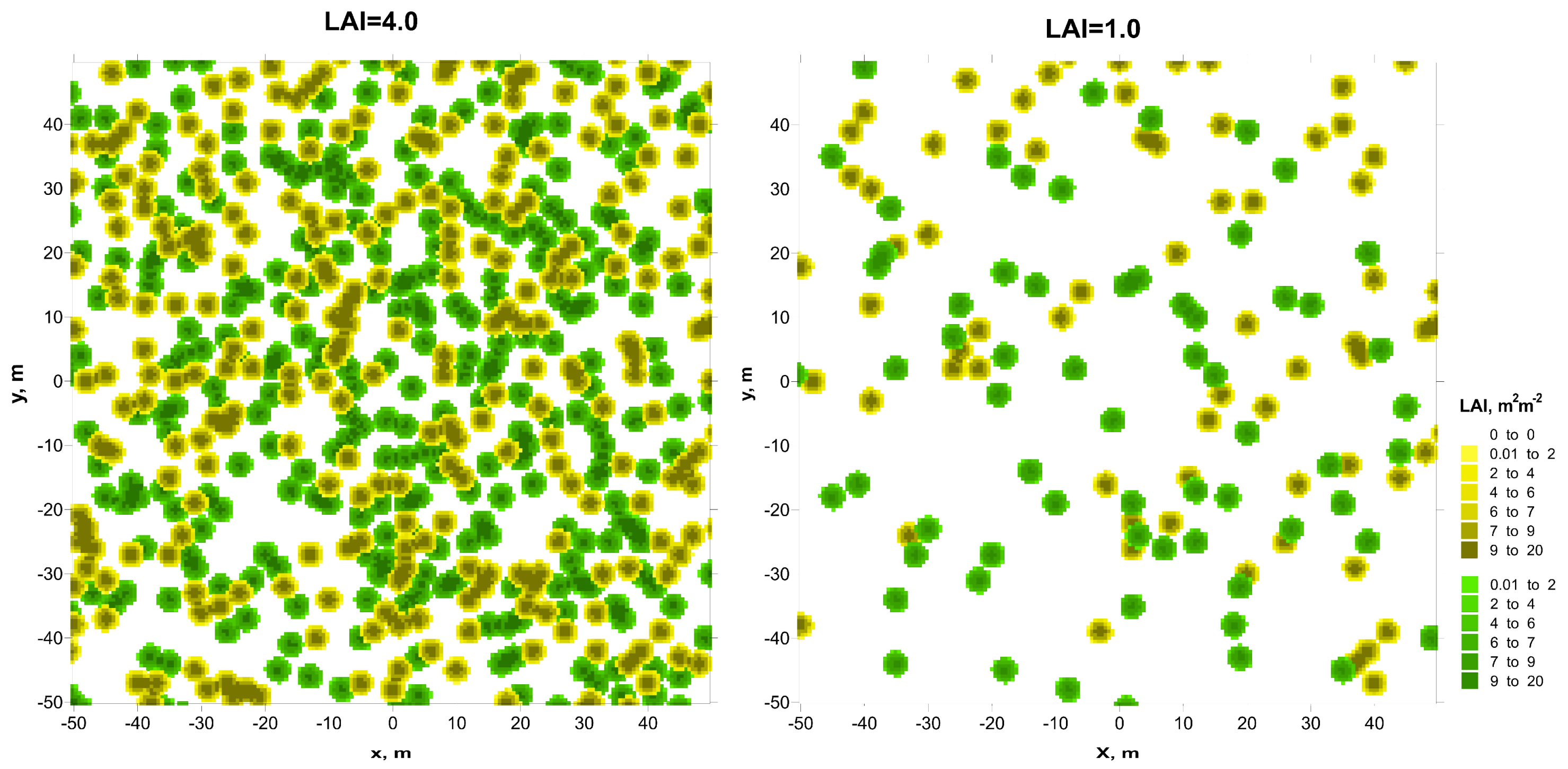
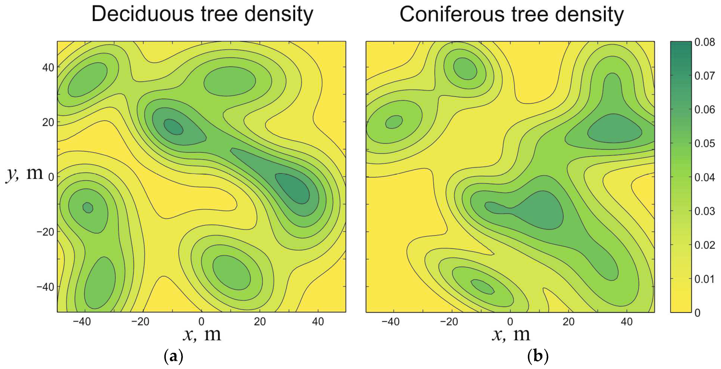
2.2. Scenarios of Numerical Experiments

To derive the possible effects of multispecies forest structure on PAR albedo (the ratio of PAR irradiance reflected to the irradiance received by a surface) and angle distribution of reflected PAR, we considered a mixed forest stand consisting of deciduous (Silver birch; Betula pendula Roth.) and coniferous (Scots pine; Pinus sylvestris L.) tree species. Such species composition is very typical for the Southern-European taiga.
All trees of different species were randomly distributed within the 100 m × 100 m modeling domain (Figure 2). The proportion of each tree species based on aboveground biomass within the modeling domain of our numerical experiments was assumed to vary between 0 and 1. Thus, the model scenarios can imitate both monospecific (pine or birch) and mixed (pine and birch trees in different proportions) forest stands. All numerical experiments were conducted for two model scenarios imitating forest stands with high (LAI = 4 m2 m−2) and low (LAI = 1 m2 m−2) stock densities. We assumed tree species have the same height (10 m) but different vertical biomass distributions.
The spatial distributions of the trees of different species were simulated using a random number generator. It was assumed that the forest stock density in case of LAI = 4 m2 m−2 was 600 trees per hectare, and in case of LAI = 1 m2 m−2 was 155 trees per hectare. To specify the locations of the trees within the modeling domain, we generated in the first step 4 arrays of 400 random numbers via a built-in compiler function. We then took half of the numbers from each array as x coordinates of a point and the other half as y coordinates. This procedure defined 800 points. After that, we generated another 800 points by interchanging the x and y coordinates. We thus obtained 1600 points for possible tree locations. As 1600 trees is too large an amount for 1 hectare we excluded some trees from our consideration. For that we generated an array of 1600 markers. The value of 600 markers (for LAI = 4 m2 m−2) related to the points of tree location were set to 1, while other markers were set to 0. Tree location points were chosen on the principle that the distance between trunks was greater than 2 m. Finally, we integrated the tree biomass distribution functions just for the tree trunk locations at points with numbers corresponding to markers equaling to 1.
The spatial distribution of biomass for individual trees was parameterized as (Figure 3):
F t r e e ( R , z ) = { max ( F l e a v e s ( R , z ) , k B F b r a n c h e s ( R , z ) ) , k B , 0 , 0 , R T R R C ( z ) ,    L T z z 0 ; R R T ,    0 z L T ; R > R C ( z ) ; z > z 0 ,  
where R = ( x x T ) 2 + ( y y T ) 2 , ( x T , y T ) are the coordinates of each tree trunk location, z is the height above the ground, z 0 = 10 m is the tree height, R T = 0.05 m is the tree trunk radius similar for all considered tree species, LT is the height of crown base counting from the ground, factor k B = 2 / 3 shows the difference in the reflection and transmission coefficients of leaves and branches for PAR, R C ( z ) is a function specifying the crown radius at height z, Fleaves(R,z), Fbranches(R,z) are the function of leaves and branches distribution within the tree crown, respectively. The expressions for these functions and the values of parameters for both tree species are detailed in Appendix B.
The optical properties of the leaves for Silver birch and Scots pine were taken from a pilot study [32]: the leaf (needle) reflection coefficient of Scots pine was 0.07, and the transmission coefficient was 0.04. The corresponding values for reflection and transmission coefficients of the Silver birch leaves were both 0.08.
The PAR albedo and the angle distribution of reflected radiation for forest stands under consideration was simulated under sunny weather conditions for different sun elevations (h0) that can be observed in the mid latitudes in the northern hemisphere in summer.
The ratio between direct and total solar radiation was derived as a function of sun elevation (h0) using results of long-term solar radiation measurements conducted at the meteorological station of Moscow State University in Moscow, Russia [33]. These measurements showed the ratio between direct (S) and diffuse (D) solar radiation can be very well described as a function of sin(h0) using a second order polynomial function (r2 = 0.99, p < 0.01): S / D = 0.159 sin 2 ( h 0 ) + 3.48 sin ( h 0 ) 0.122 .
To derive the effects of soil optical properties on reflected and absorbed PAR, all modeling experiments were conducted for both dark (ρs = 0.01) and light (ρs = 0.20) soils.
We also assumed in our numerical experiments that the atmospheric absorption term is negligible [22].

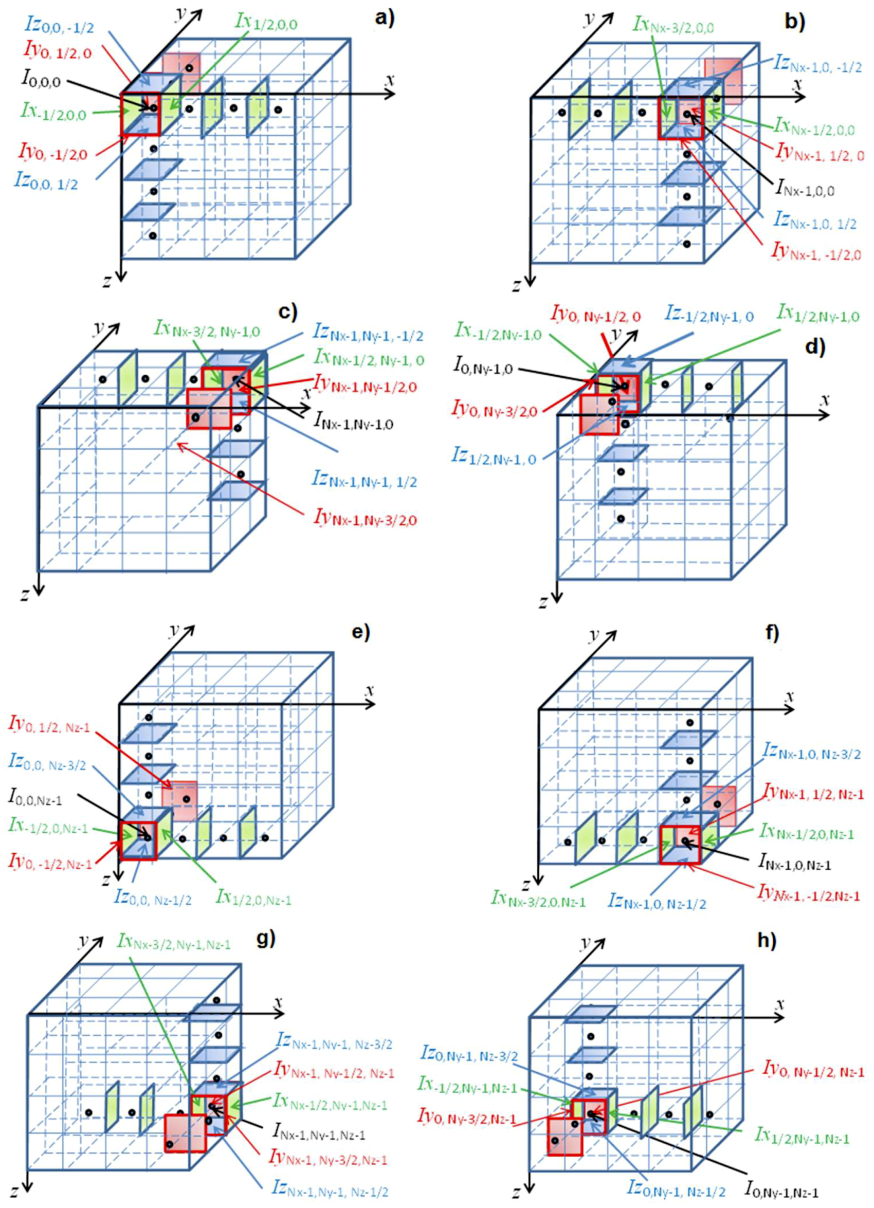
2.3. The Numerical Scheme

The numerical scheme suggested by Myneni et al. [34] was used to solve the integro-differential Equation (1). The equation was solved using discrete ordinates method. It is based on splitting the angular variable Ω into a smaller number of directions. Here, the discretization was performed using the Gauss–Markov quadrature formulae of the 17th order [35]. Equation (1) was solved for each of the discrete ordinates Ω m ,    m = 0       109 via the iteration procedure [34].
We selected the following boundaries for our modeling domain considering the horizontal and vertical dimensions of the selected forest plot (100 m × 100 m, tree height—10 m): 54   m x , y 54   m ,     0   m z 11.5   m . The choice of domain dimensions was governed by the need to step back from the edges of the hectare domain under consideration to reduce the influence of the boundary conditions. The choice of domain was also constrained by computer resources. The entire modeling domain was also divided into uniform grid cells: ( x i , y j , z k ) , i = 0 , N x 1 ¯ , j = 0 , N y 1 ¯ , k = 0 , N z 1 ¯ each of which was characterized by a specific density of photosynthesizing and non-photosynthesizing phyto-elements (branches, stem) for each tree species. The OZ-axes was directed from the top of our modeling domain to its bottom.
We use the notation I x i 1 2 ,    j ,    k ( n + 1 ) ( Ω m ) , i = 0 , N x ¯ , j = 0 , N y 1 ¯ and k = 0 , N z 1 ¯ to specify the radiance spreading along the direction Ωm at the face of (i,j,k) grid cell perpendicular to OX axis at (n + 1)th iteration. Similarly, notations I y i ,    j 1 2 ,    k ( n + 1 ) ( Ω m ) , i = 0 , N x 1 ¯ , j = 0 , N y ¯ and k = 0 , N z 1 ¯ for radiance at the grid cell face perpendicular to OY axis; I z i ,    j ,    k 1 2 ( n + 1 ) ( Ω m ) , i = 0 , N x 1 ¯ , j = 0 , N y 1 ¯ , and k = 0 , N z ¯ at the cell face perpendicular to OZ axis; and I i , j , k ( n + 1 ) ( Ω m ) for the central-cell value.
Equation (1) can be rewritten in finite difference form as:
μ m Δ z ( I z i ,    j ,    k + 1 2 ( n + 1 ) ( Ω m ) I z i ,    j , k 1 2 ( n + 1 ) ( Ω m ) ) + η m Δ y ( I y i ,    j + 1 2 , k ( n + 1 ) ( Ω m ) I y i ,    j    1 2 , k ( n + 1 ) ( Ω m ) ) + + ξ m Δ x ( I x i + 1 2 , j , k ( n + 1 ) ( Ω m ) I x i , j 1 2 , k ( n + 1 ) ( Ω m ) ) + σ ( r i , j , k , Ω m ) I i , j , k ( n + 1 ) = J i , j , k ( n ) ( Ω m ) ,
where r i , j , k = { x i , y j , z k } ,
J i , j , k ( n ) ( Ω m ) = 4 π I i , j , k ( n ) ( r i , j , k , Ω ) σ s λ ( r i , j , k , Ω Ω m ) d Ω + σ s λ ( r i , j , k , Ω 0 Ω m ) Q 0 , λ ( r i , j , k )  
The value of the integral on the right-hand side was obtained numerically as:
4 π I i , j , k ( n ) ( r i , j , k , Ω ) σ s λ ( r i , j , k , Ω Ω m ) d Ω = 4 π m = 0 109 I i , j , k ( n ) ( r i , j , k , Ω m ) σ s λ ( r i , j , k , Ω m Ω m ) W ( Ω m )  
with discrete ordinates Ωm and weights W ( Ω m ) taken according to Gauss–Markov quadrature formula of 17th order [35].
In order to link unknown variables in (2) we used the equalities called the diamond difference relations (DD method):
I i , j , k ( n + 1 ) ( Ω m ) = 1 2 ( I x i 1 2 ,    j ,    k ( n + 1 ) ( Ω m ) + I x i + 1 2 ,    j ,    k ( n + 1 ) ( Ω m ) ) ,     I i , j , k ( n + 1 ) ( Ω m ) = 1 2 ( I y i ,    j 1 2 ,    k ( n + 1 ) ( Ω m ) + I y i ,    j + 1 2 ,    k ( n + 1 ) ( Ω m ) ) , I i , j , k ( n + 1 ) ( Ω m ) = 1 2 ( I z i ,    j ,    k    1 2 ( n + 1 ) ( Ω m ) + I z i ,    j ,    k + 1 2 ( n + 1 ) ( Ω m ) ) .
Excluding I z i ,    j ,    k + 1 2 ( n + 1 ) , I y i ,    j + 1 2 , k ( n + 1 ) , and I x i + 1 2 ,    j ,    k ( n + 1 ) from (2) and (3) we came to the following expression:
I i , j , k ( n + 1 ) ( Ω m ) = J i , j , k ( n ) ( Ω m ) + 2 | μ m | Δ z I z i ,    j , k 1 2 ( n + 1 ) ( Ω m ) + 2 | η m | Δ x I y i ,    j 1 2 , k ( n + 1 ) ( Ω m ) + 2 | ξ m | Δ x I x i 1 2 ,    j , k ( n + 1 ) ( Ω m ) σ ( r i , j , k , Ω m ) + 2 | μ m | Δ z + 2 | ξ m | Δ y + 2 | η m | Δ x .  
Then we completed the following steps:
(1) In the first step we determined the radiance spreading along the directions Ω m = { ξ m , η m , μ m } , ξ m 2 + η m 2 + μ m 2 = 1 with ξ m > 0 , η m 0 , μ m 0 (the first octant). In this case the values I x 1 2 , 0 , 0 ( n + 1 ) ( Ω m ) , I y 0 , 1 2 ,    0 ( n + 1 ) ( Ω m ) , I z 0 ,    0 , 1 2 ( n + 1 ) ( Ω m ) were known from the boundary conditions. Then the value of the radiance for i = j = k = 0 was obtained from relation (4).
(2) Taking into account the known value I 0 , 0 , 0 ( n + 1 ) ( Ω m ) from (3) we expressed I z 0 ,    0 ,     1 2 ( n + 1 ) ( Ω m ) , I y 0 ,     1 2 , 0 ( n + 1 ) ( Ω m ) , I x    1 2 ,    0 ,    0 ( n + 1 ) ( Ω m ) —the values for all indices i, j, and k fulfilling the condition i + j + k = 1.
(3) Now the central-cell values I i , j , k ( n + 1 ) ( Ω m ) for the indices with i + j + k = 1 can be obtained from (4). And so on: taking into account the known value I i , j , k ( n + 1 ) ( Ω m ) from (3) we expressed I z i ,    j ,    k + 1 2 ( n + 1 ) ( Ω m ) , I y i ,    j + 1 2 , k ( n + 1 ) ( Ω m ) and I x i + 1 2 ,    j ,    k ( n + 1 ) ( Ω m ) for all indices i, j, and k satisfying the relation i + j + k = c , where c consistently takes the values 1 ,    2 ,    ,    N x + N y + N z 3 .
The calculation procedure is schematically shown in Figure 4a.
(5) The same procedure was used for calculating the second octant ordinates: ξ m 0 ,    η m > 0 ,    μ m 0 with the values I x N x 1 2 , 0 , 0 ( n + 1 ) ( Ω m ) , I y N x 1 , 1 2 ,    0 ( n + 1 ) ( Ω m ) , I z N x 1 ,    0 , 1 2 ( n + 1 ) ( Ω m ) taken from the boundary conditions. We obtain I i , j , k ( n + 1 ) ( Ω m ) from (4) at each step and then express I z i ,    j ,    k + 1 2 ( n + 1 ) , I y i ,    j + 1 2 , k ( n + 1 ) , I x i + 1 2 ,    j ,    k ( n + 1 ) from (3) for all indices i, j, k fulfilling the conditions N x 1 i + j + k = c , where c = 1 ,    2 ,    ,    N x + N y + N z 3 . (Figure 4b).
(6) The calculations were similarly carried out for other octants (see Figure 4c–h).
(7) The flux of solar radiation at each point ( x i , y j , z k ) was calculated as the total intensity of scattered radiation in each direction Ω m and summed with the intensity of direct solar radiation.

2.4. The Inverse Problem Statement to Retrieve the Forest Species Composition

Let us assume that ( x , y ) D is the modeling domain with randomly distributed trees of different species. The functions ρ 1 ( x , y ) and ρ 2 ( x , y ) determine the spatial distributions of different tree species (trees per hectare) (here the subscripts “1” and “2” indicate deciduous and coniferous tree species, respectively) within the modeling domain. Let us also assume that we have known functions I 1 ( φ , θ ) and I 2 ( φ , θ ) describing the radiation intensity that is reflected from some average tree of each species in the direction determined by spherical coordinates ( φ , θ ) .
Thus, for some very small pixel ds specified by coordinates ( x , y ) on which both types of trees species are grown, we can calculate the radiation intensity that is measured by a PAR sensor located at some point with coordinates ( x s , y s , z s ) along the corresponding solid angle dΩ under which the surface element ds is visible: d Ω d Ω ( x , y , x s , y s , z s , d s ) k ( x , y , x s , y s , z s ) d s .
The total radiation intensity I reflected from the surface element ds is a function of angle coordinates φ ( x , y , x s , y s ) arctan y s y x s x and θ ( x , y , x s , y s , z s ) arctan ( x s x ) 2 + ( y s y ) 2 z s :
I ( φ ( x , y , x s , y s ) , θ ( x , y , x s , y s , z s ) ) d Ω ( x , y , x s , y s , z s , d s ) = = I 1 ( φ ( x , y , x s , y s ) , θ ( x , y , x s , y s , z s ) ) ρ 1 ( x , y ) d s + I 2 ( φ ( x , y , x s , y s ) , θ ( x , y , x s , y s , z s ) ) ρ 2 ( x , y ) d s .
In coordinates (x,y,z) this relation can be rewritten as:
I 1 ( x , y , x s , y s , z s ) ρ 1 ( x , y ) d s + I 2 ( x , y , x s , y s , z s ) ρ 2 ( x , y ) d s = I ( x , y , x s , y s , z s ) k ( x , y , x s , y s , z s ) d s .  
The inverse problem can be posed as follows: it is necessary to determine the functions ρ 1 ( x , y ) , ρ 2 ( x , y ) W 2 2 ( D ) from measured values of the function I ( φ , θ , x s , y s , z s ) L 2 ( D ) along some trajectory above a forest canopy ( x s = x s ( p ) , y s = y s ( p ) , and z s = z s ( p ) , p [ p 1 , p 2 ] ).

2.5. The Model Algorithm for Inverse Problem Solving

The model algorithm can be divided into seven sequential steps:
1. In the first step we define the domain D on which model functions ρ 1 ( x , y ) and ρ 2 ( x , y ) are retrieved as a rectangle with following dimensions: D { ( x , y ) :    L x x R x ,    L y y R y } .
2. We divide region D into N x × N y grid cells, at the center of each we put the node. As a result, we obtain a X N x × Y N y mesh with a step h x = ( R x L x ) / N x with respect to the variable x and the step h y = ( R y L y ) / N y with respect to y:
X N x × Y N y { ( x n x , y n y ) ,    1 n x N x ,    1 n y N y :     x n x = L x + h x 2 + ( n x 1 ) h x ,    y n y = L y + h y 2 + ( n y 1 ) h y }  
3. We introduce a uniform grid on the part of the trajectory along which the measurements of functions I 1 and I 2 were made. For simplicity, we assume that p [ 0 , 1 ] , x s = x s ( p ) L s + ( R s L s ) p , y s = y s ( p ) l y = c o n s t , z s = z s ( p ) l z = c o n s t . Thus, the corresponding mesh is uniform and co-oriented in space parallel to the coordinate axis Ox. The related mesh S N p with N p 1 intervals of length h s = ( R s L s ) / ( N p 1 ) takes the form: S N p { s n p ,    1 n p N p :    s n p = L s + ( n p 1 ) h s } .
4. We calculate the values of the functions I 1 ( φ , θ ) and I 2 ( φ , θ ) :
I 1 ( φ ( x n x , y n y , s n p , l y ) , θ ( x n x , y n y , s n p , l y , l z ) ) I 1 n x , n y , n p , I 2 ( φ ( x n x , y n y , s n p , l y ) , θ ( x n x , y n y , s n p , l y , l z ) ) I 2 n x , n y , n p ,
where φ ( x n x , y n y , s n p , l y ) = { arctan l y y n y s n p x n x , if    l y y n y 0    and    s n p x n x 0 , arctan l y y n y s n p x n x + 2 π , if    l y y n y < 0    and    s n p x n x 0 , arctan l y y n y s n p x n x + π , if    s n p x n x < 0 ,
θ ( x n x , y n y , s n p , l y , l z ) = arctan ( s n p x n x ) 2 + ( l y y n y ) 2 l z for all n x = 1 , N x ¯ , n y = 1 , N y ¯ , n p = 0 , N p ¯ .
5. We calculate the values of model functions ρ 1 ( x , y ) and ρ 2 ( x , y ) : ρ 1 ( x n x , y n y ) ρ 1 n x , n y , ρ 2 ( x n x , y n y ) ρ 2 n x , n y , for all n x = 1 , N x ¯ , n y = 1 , N y ¯ .
6. The main equation (5) can be rewritten as:
I 1 n x , n y , n p ρ 1 n x , n y h x h y + I 2 n x , n y , n p ρ 2 n x , n y h x h y = I ˜ n x , n y , n p ,  
and for all n x = 1 , N x ¯ , n y = 1 , N y ¯ , n p = 0 , N p ¯ that provides the system of linear algebraic equations (SLAE) in the form
A X = Y
with matrix of operator A having a dimension N x N y N p × 2 N x N y and vector X of length 2 N x N y , with non-zero components as follows:
A ( n p 1 ) N x N y + ( n x 1 ) N y + ( n y 1 ) + 1 , ( n x 1 ) N y + ( n y 1 ) + 1 = I 1 n x , n y , n p h x h y , for    n x = 1 , N x ¯ ,    n y = 1 , N y ¯    and    n p = 1 , N p ¯ , A ( n p 1 ) N x N y + ( n x 1 ) N y + ( n y 1 ) + 1 , N x N y + ( n x 1 ) N y + ( n y 1 ) + 1 = I 2 n x , n y , n p h x h y , for    n x = 1 , N x ¯ ,    n y = 1 , N y ¯    and    n p = 1 , N p ¯ ,
X n = { ρ 1 [ ( n 1 ) / N y ] + 1 , { ( n 1 ) / N y } + 1 ,   if    n = 1 , N x N y ¯ , ρ 2 [ ( n 1 N x N y ) / N y ] + 1 , { ( n 1 N x N y ) / N y } + 1 ,   if    n = N x N y + 1 , 2 N x N y ¯ .  
Square brackets mean a whole part of the expression and figured brackets mean the decimal part.
As a result, via (6) using the model values of functions ρ 1 ( x , y ) and ρ 2 ( x , y ) on the introduced grid X N x × Y N y as the components of vector X m o d e l , we simulate a model vector Y of input data having the length N x N y N p according to the following algorithm:
(a) Error simulation of operator A elements (that means a model error):
A h    m , n = A m , n ( 1 + ξ h 100 % )     for    all   m = 1 , N x N y N p ¯ ,    n = 1 , 2 N x N y ¯  
where ξ is a uniformly distributed on the segment [−1,1] random value, h is a given error in percent.
(b) Calculation of vector Y from the ratio:
A h X m o d e l = Y
(c) Error simulation of Y components (that means the error of experimental data):
Y δ m = Y m ( 1 + ξ δ 100 % )      for    m = 1 , N x N y N p ¯ ,  
where ξ is a uniformly distributed random value on the segment [-1,1], δ is a given error in percent.
7. We seek for the solution of (6) with simulated vector Y δ by the least square method:
X = ( A T A ) 1 A T Y δ
If the solution of this equation is unstable, the regularizing algorithm can be used. It can be done, for instance, by using the Tikhonov regularizing algorithm based on the minimization of smoothing functional [36]. In this case the solution of (6) can be found as a minimum of Tikhonov functional M α [ x ] (smoothing functional):
M α [ X ] = A X Y δ 2 + α R X 2 ,
where α is the regularization parameter, R is the “smoothing operator” (for simplicity while solving the model problem, we shall use R = E, where E is a unit operator). The extremal of this functional can be found as the solution of SLAE:
( A T A + α R T R ) X = A T Y δ 1 A T Y δ
In case the solution of (7) is stable with respect to the model errors (h) and the errors of input data (δ) we have α = 0. Otherwise if the solution of (7) is unstable with respect to the mentioned errors, then the choice of the regularization parameter α must be consistent with the errors δ of the input data Yδ and h of the operator A. Such a choice can be made using, e.g., the generalized discrepancy principle [36]:
ρ ( α ) = 0 ,    where    ρ ( α ) = A X α Y δ 2 ( Δ + H X α ) 2 μ 2  
Here X α is the extremal of the functional M α [ X ] ( M α [ X α ] = inf M α [ X ] ); Δ > 0 is the root-mean-square error of the specification ( Y δ ) in right-hand side of (6):
Δ 2 = m = 1 N x N y N p ( Y m ξ δ 100 % ) 2 ;
H > 0 is the root-mean-square error of operator A specification:
H 2 = m = 1 N x N y N p n = 1 2 N x N y ( A m , n ξ h 100 % ) 2 ;
where μ is the measure of incompatibility of SLAE (6), i.e., μ = inf A h X Y δ = { A h X α Y δ α = 0 } .

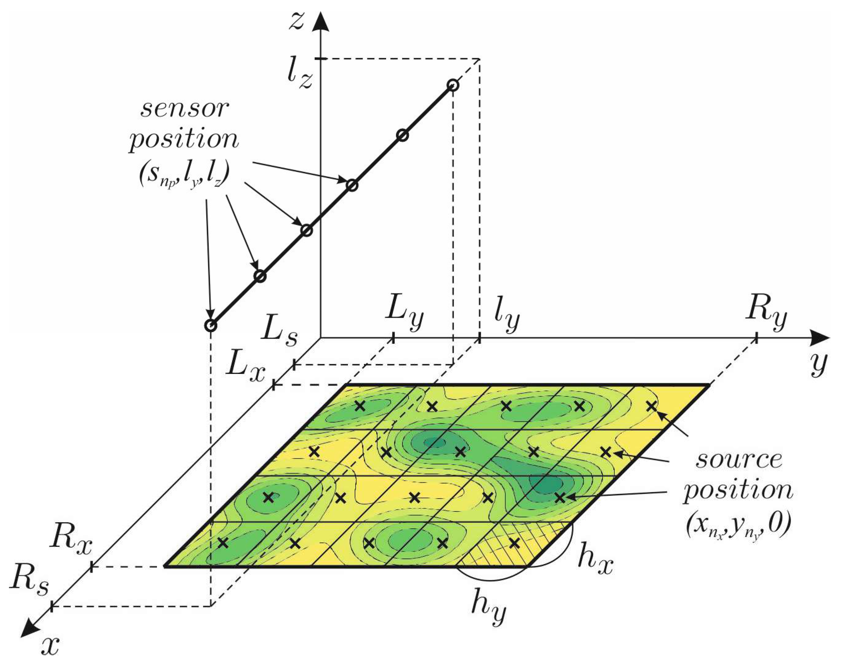
2.6. Modeling Design for Inverse Problem Solution

To retrieve the forest species composition within our modeling domain D (Figure 2) with spatial dimensions (in meters) L x = 50 , R x = 50 , L y = 50 , R y = 50 , let us select the segment of the straight line defined by the parameters L s = 60 , R s = 60 , l y = 10 , l z = 200 . This could correspond to the flight line of a helicopter, aircraft or drone carrying a PAR sensor 200 m above the forest (Figure 5).
The distribution of each tree species in a mixed forest stand is usually discrete. In our case, in order to test the suggested algorithm, we assumed the smoothed discrete distributions of different tree species within the modeling domain and described them by functions ρ 1 ( x , y ) and ρ 2 ( x , y ) specifying the density (trees per hectare) of each type of tree species (Figure 6).
The values of functions I 1 ( φ , θ ) and I 2 ( φ , θ ) where I 1 , 2 ( φ , θ ) I 1 , 2 ( φ ( x n x , y n y , s n p , l y ) , θ ( x n x , y n y , s n p , l y , l z ) ) I 1 , 2 n x , n y , n p for each sensor position ( s n p , l y , l z ) along the selected trajectory and for each node of the mesh ( n x , n y ) were determined as radiation scattered by single trees along the direction ( φ , θ ) , 0 φ < 360 ° , 0 θ < 90 ° into the upper hemisphere. The reflected radiation was calculated using the 3D model, based on the assumption that the sun elevation was 30° ( h 0 = 30 ° ) and the sun rays were incident from the south.

3. Results and Discussion

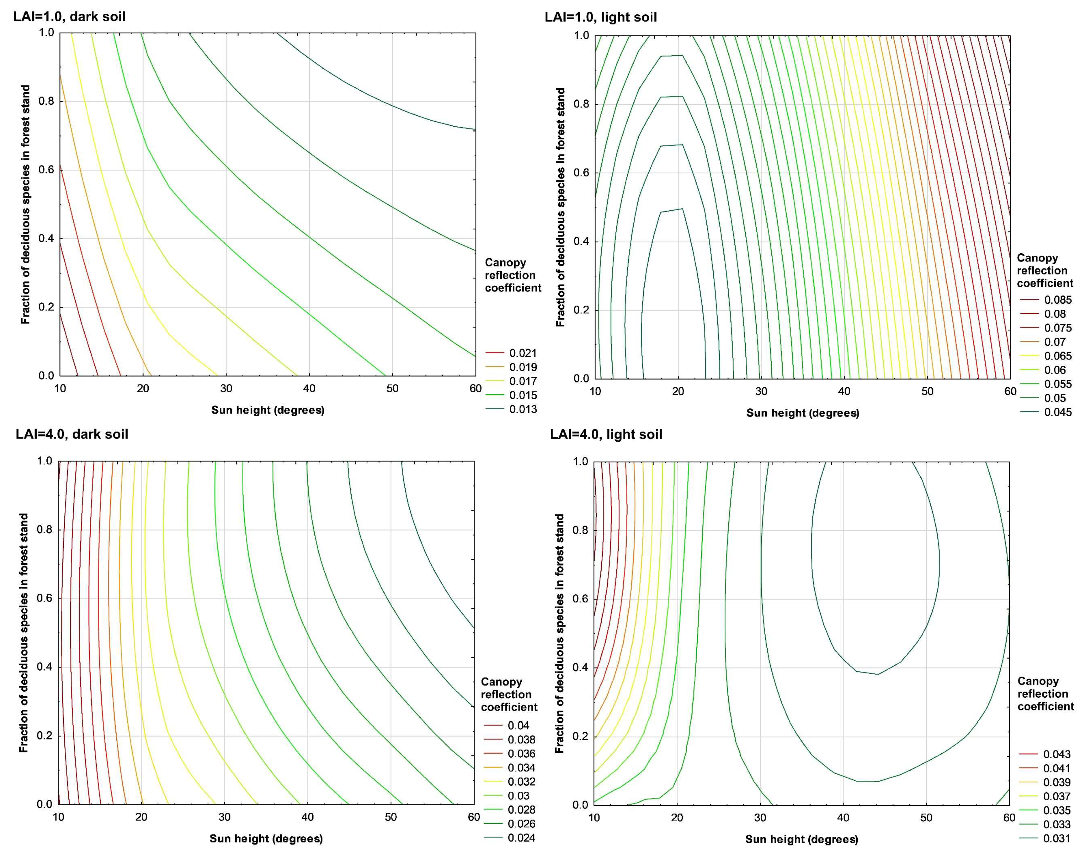
3.1. Reflection of PAR for Mixed Forest Stand

Numerous experimental and modeling studies during recent decades showed that PAR albedo measured by different remote sensing equipment or by devices installed at meteorological towers can be broadly used to estimate canopy structure and architecture, surface net radiation, gross and net primary production, etc. [25,37,38,39,40]. Let us consider the possible effects of the change of forest species composition on variation of reflected PAR.
The numerical experiments provided using the 3D radiative transfer model showed a clear dependence of PAR albedo of both monospecific and mixed forest stands on canopy density (LAI), sun elevation, and soil reflection properties (Figure 7). The canopy albedo for sparse forest canopy and dark soils reached maximal values under low sun elevation, and minimal values under high sun elevation. This is because sunbeams travel longer distances through the forest canopy before interacting with the soil surface. This results in higher scattered direct solar radiation within the plant canopy; therefore, there is a higher vegetation contribution to the total forest reflection. The overall canopy reflection also increased with a higher proportion of birch trees in the forest canopy. This is mainly due to higher birch leaf reflection and transmission coefficients compared with pine. In the case of light soil, the dependence of forest albedo on sun elevation has the opposite effect. Simulated local minimums of forest albedo at h0 = 20° can be explained by a reduced contribution of reflected direct solar radiation from light soils to the total forest albedo, joint effects of canopy architecture, and the optical properties of the soil and plant phyto-elements (leaves, branches, stem).
In the case of a dense forest canopy (LAI = 4.0 m2 m−2), the albedo gradually increases with increasing sun elevation. The rate of this increase is slightly higher for dark soils. The clear dependence of albedo on species composition mainly manifested under high sun elevations. The forest canopy with a higher proportion of birch trees was characterized by higher albedo. Under low sun elevation (h0 < 20°), the albedo was less dependent on species composition. A local minimum of canopy reflection under a sun height of ~45° can be caused by the influence of forest canopy architecture (spatial leaf area distribution; orientation of leaf blades) and the optical properties of the tree species and soil surface.
Summarizing all obtained results, it is possible to emphasize a high sensitivity of PAR albedo to forest canopy density, soil properties, and sun conditions. The dependence of forest albedo on the proportion of deciduous and coniferous species in a forest stand, except at low sun elevations (h0 < 25–30°), was also shown. The results of our numerical experiments agreed well with available experimental and modeling data obtained by different scientific teams for various plant canopy types. In particular, Knyazikhin et al. [22] and Gravenhorst et al. [23] showed a clear impact of sun elevation on the PAR albedo of monospecific old-grown spruce forest in Solling, Germany. Maximal albedo was observed in the morning and evening, and the minimal values were close to noon. The soil had a minor impact on albedo because of a very dense overstory and grassy understory that almost completely covered the soil surface. Similar results were also obtained during the field observations provided by Pinker et al. (1980) [41] in a tropical dry evergreen forest in Southeast Asia and by Giambelluca et al. (1997) [42] at several forest and shrub locations in Amazonia.
Lower albedo at higher sun elevations can be explained by deeper penetration of solar photons into the vegetation cover under a lower solar zenith angle, more frequent interaction of solar photons with plant components, and higher probability to be absorbed by plant elements and soil surface before escaping back into the atmosphere [43,44]. Another factor contributing to the change in surface albedo with solar elevation angle is the soil surface fraction illuminated by direct solar beams. At the highest sun positions (i.e., highest sun elevation angle or lowest solar zenith angle), the contribution of directly illuminated soil surface into the total reflected solar radiation reach maximum values. As solar zenith angle and shadow fraction increase, the proportion of directly illuminated soil surface decrease and the contribution of the soil surface to surface albedo also decrease.
In discussing the possible effects of forest canopy architecture on radiative transfer characteristics, it is also necessary to consider the influence of leaf inclination on light reflection. In particular, Simioni et al. (2013) [45] showed that the light reflection and absorption of mixed deciduous and coniferous forests is highly sensitive to leaf blade inclination of different tree species, and erroneous assumptions about leaf inclination lead to larger uncertainties when modeling heterogeneous mixed canopies. In our numerical experiments we assumed that both our model trees (birch and pine) have the same spherical angular orientation of phyto-elements. Thus, possible uncertainties in estimating the canopy albedo, due to differences in angular orientation of phytoelements between different species in our numerical experiments, can be ignored.
Another factor that can highly influence the forest canopy albedo is the surface topography. Kranigk et al. (1994) [46] and Knyazikhin et al. (1996, 2005) [21,31] performed experimental and modeling studies on radiation regime in a spruce forest stand growing in the Harz Mountains in Central Germany. It was shown that complex topography can result in strong redistribution of reflected and penetrated solar radiation depending on the surface slope and aspect characteristics, and in turn, can influence forest net primary production and tree growth. In our numerical experiments, we considered the modeling scenario assuming only a flat topography. Thus, any uncertainties in radiation reflection characteristics, due to complex topography, can be ignored.

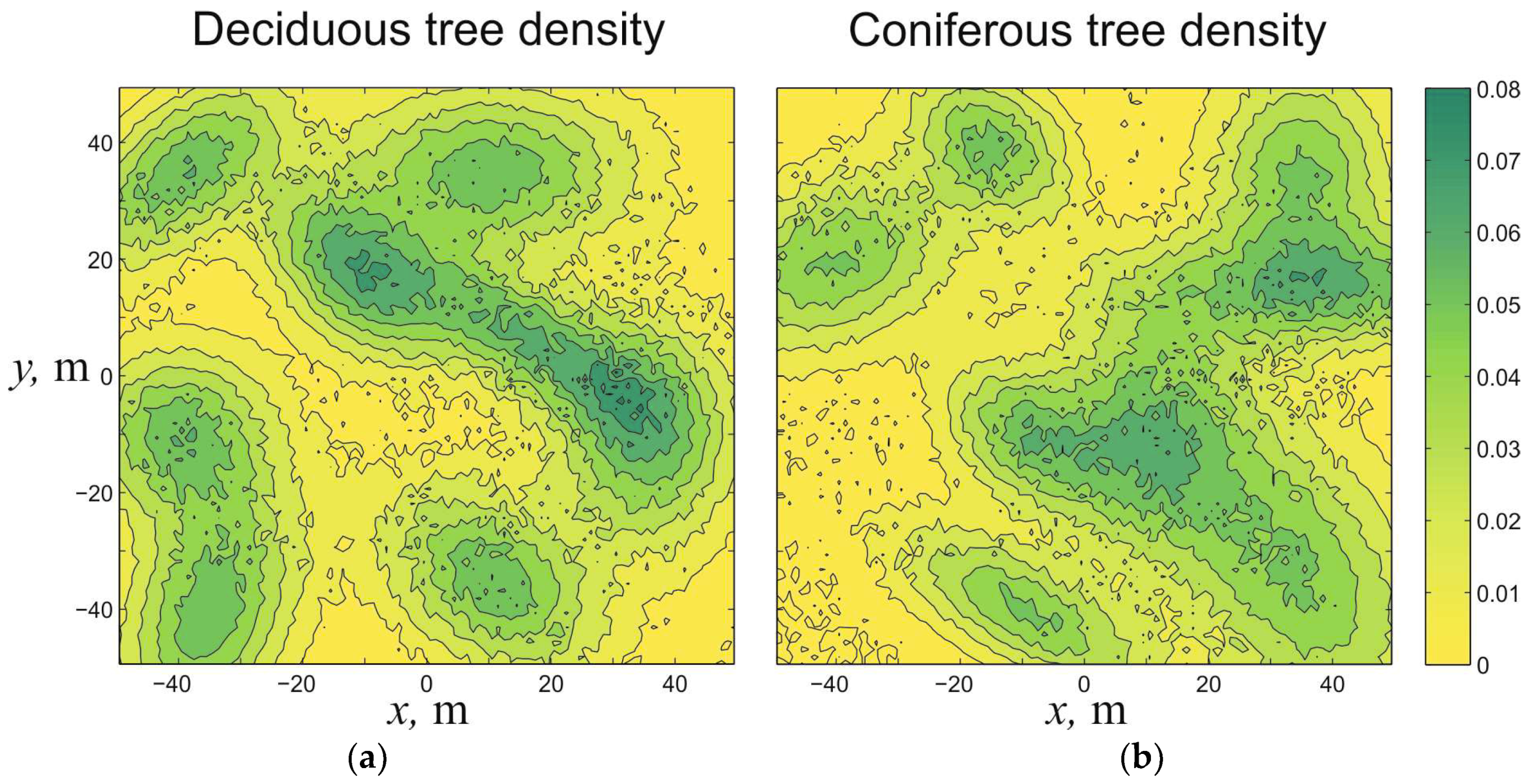
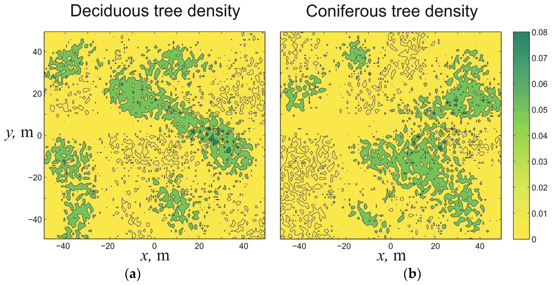
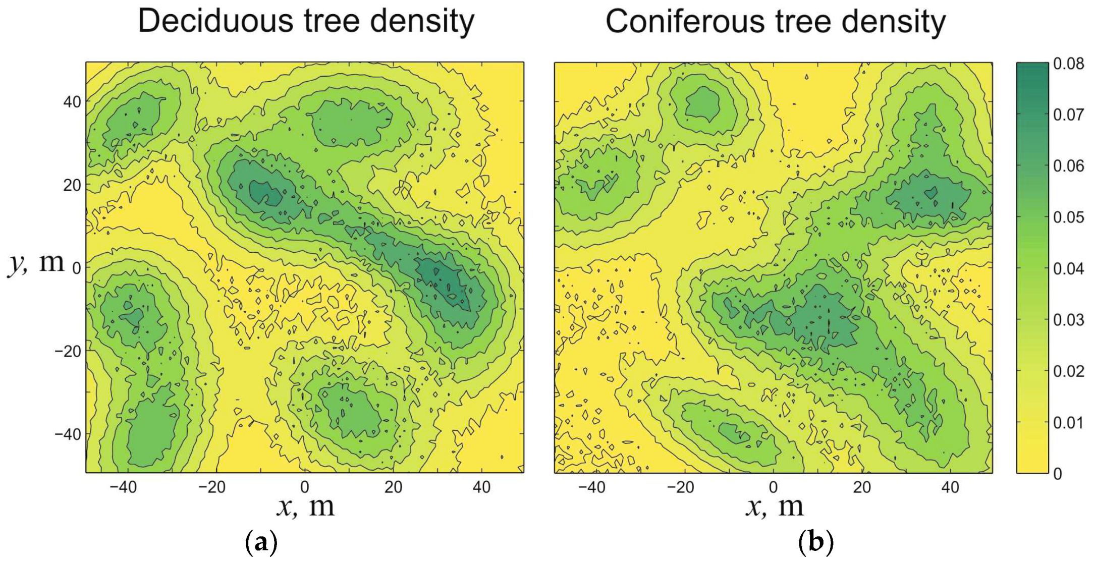
3.2. Retrieving Species Composition of a Mixed Forest Stand from Canopy Reflectance Properties

The results of numerical experiments to retrieve the density of deciduous and coniferous tree species ( ρ 1 ( x , y ) and ρ 2 ( x , y ) ) in a mixed forest stand from canopy reflection properties are shown in Figure 8, Figure 9 and Figure 10. As can be seen, with an increase of the error δ and h with which the canopy reflection measurements that can be carried out, the retrieving accuracy of the unknown functions drastically decreases. Figure 8 and Figure 9 represent examples of species composition retrieved for measurement error levels of ( δ ; h ) = ( 1 ; 1 ) % and ( δ ; h ) = ( 5 ; 6 ) % (the last is consistent with the model error mentioned in [23]) with a similar number of measurement points N p ). However, even with a sufficiently large error level in the measured signal and model error, it is possible to retrieve the unknown functions when measurements are carried out at a larger number of points. Figure 9 and Figure 10 show a comparison of the results for the same error levels of ( δ ; h ) = ( 5 ; 6 ) % in the experimental data with N p = 10 and N p = 500 measurement points.
The statements made above are supported by the following results. Figure 11 shows the dependence of the root-mean-square error ( s = X i n v X mod e l 2 N x N y ) for the components of the reconstructed vector X i n v = ( A T A + α R T R ) 1 A T Y δ in case α = 0 on the error levels δ of the input data and h of the model (for a fixed number of measurement points N p ). From this graph it can be seen that a decrease in the error δ with which the canopy reflection measurements are carried out, and the model error h, resulted in increase of the accuracies of vector X i n v reconstruction, and hence, the grid values of functions ρ 1 ( x , y ) and ρ 2 ( x , y ) . This means that X i n v X m o d e l when ( δ ; h ) 0 . So, the suggested inverse problem statement is stable and the corresponding algorithm is therefore regularizing [36].
Figure 12 shows the dependence of the root-mean-square error in the components of the reconstructed vector X i n v on the number of measurement points N p (for a fixed error level δ in the input data and h in the model). From this graph it is clearly seen that an increase of the input data volume (determined by the number N p of the measurement points) resulted in an increase of accuracies of vector X i n v reconstruction and hence, the grid values of functions ρ 1 ( x , y ) and ρ 2 ( x , y ) . These results support the notion of increasing the number of measuring points as much as possible.

3.3. Other Possible Ways to Reconstruct the Proportions of Different Tree Species in a Mixed Forest from Canopy Reflection Using the 3D Model

During recent decades, many algorithms have been suggested to quantify structural and optical aspects of vegetation canopies from remote sensing [25,28,45,46,47,48]. The problem of mapping forest composition in mixed forest stands using remote sensing data is still open. Several studies used hyperspectral and/or LiDAR data from LiCHy (Hyperspectral sensors, LiDAR and CCD (Charge-Coupled Device) camera) airborne systems to classify tree species composition in mixed forests [49] or high-resolution imagery for mapping forest cover types [50,51,52,53].
As shown in the previous section, the task to retrieve forest species composition from LAI, canopy, and soil reflection is not trivial, due to the multivariate relationships between solar radiation reflection, scattering coefficients, and tree species composition (different proportions of deciduous and coniferous trees in mixed forest stand) under various LAI and soil reflection. The mean canopy albedo is relatively insensitive to changes in the proportion of different species in a forest stand—especially in the case of dense forest and low sun elevations (Figure 7). However, the main conclusion that can be drawn from Section 3.2 is that the forest stand species composition can be reconstructed from information on canopy reflection properties.
Let us consider some other possibilities to solve this inverse problem using this 3D model and find effective numerical algorithms that would allow us to reconstruct forest species composition from other structural and optical properties of a plant canopy and soil (LAI, leaf reflection and transmission, soil reflection, etc.).
1. The functions ρ 1 ( x , y ) ,     ρ 2 ( x , y ) H ( D ) are known from measurements of intensity I ( φ , θ , x s , y s , z s ) L 2 ( D ) at a single fixed point ( x s , y s , z s ) .
This formulation of the problem is physically undetermined because it restores two functions ρ 1 and ρ 2 of two variables ( x , y ) with one function I of two variables ( φ , θ ) . In other words, for a fixed set of parameters ( x , y , x s , y s , z s ) , we can write only one equation with two unknown values. Thus, for all possible ( x , y ) D determining all viewing angles ( φ , θ ) after digitization of the corresponding domains we obtain a system of equations with twice as many unknown values as equations. Consequently, this formulation will be incorrect according to Hadamard, regarding the lack of uniqueness of the solution.
However, in case of the available and sufficiently precise a priori information about the functions ρ 1 and ρ 2 belonging to a certain space (class of functions) H, we can reformulate the problem as determining the functions ρ 1 ( x , y ) ,     ρ 2 ( x , y ) H ( D ) that realize minimum of the functional F [ ρ 1 , ρ 2 ] = D ( I 1 ρ 1 + I 2 ρ 2 I k ) 2 d s with the assumption that H ( D ) is some compact set of functions, e.g., monotonic functions, piecewise-convex functions, functions of bounded variation, etc. Examples of analogous problem statements using a priori information on the desired functions are available in some studies [36,54,55,56].
Thus, the task to find ρ 1 ( x , y ) ,     ρ 2 ( x , y ) H ( D ) can be rewritten in the following form:
{ ρ 1 , ρ 2 } = arg min ρ 1 , ρ 2 H ( D ) F [ ρ 1 , ρ 2 ] arg min ρ 1 , ρ 2 H ( D ) D ( I 1 ρ 1 + I 2 ρ 2 I k ) 2 d s .  
The advantage of this approach is that (i) it is possible to find a solution to the problem having the function of radiation intensity distribution measured at a single point, and (ii) the formulation of the problem can be correct both in terms of uniqueness and in terms of stability of the solution. The disadvantages of this approach is that (i) for the case of each compact set H ( D ) it is necessary to conduct theoretical analysis of the corresponding problem correctness with respect to the uniqueness and stability of its solution; (ii) the a priori information on the form of the set H ( D ) may not be available.
This approach is not yet physically undetermined because we obtain basic additional information from the assumption that the recoverable functions have certain physical properties.
2. The functions ρ 1 ( x , y ) ,     ρ 2 ( x , y ) are known from measured values of function I ( φ , θ , x s , y s , z s ) L 2 ( D ) at the two fixed points ( x s , y s , z s ) 1 and ( x s , y s , z s ) 2 .
We have in this case a physically determined problem because it demands recovery of two functions ρ 1 and ρ 2 of two variables ( x , y ) from two known functions of I 1 and I 2 of two variables ( φ , θ ) : I n is the set of radiation intensities values obtained from point ( x s , y s , z s ) n ,    n = 1 , 2 .
Within this approach, it is no longer necessary to consider faithful a priori information about the form of the set H ( D ) . It is sufficient to assume that ρ 1 ( x , y ) ,     ρ 2 ( x , y ) W 2 2 ( D ) and the problem to determine ρ 1 and ρ 1 can be solved in a classical way (e.g., the least square method):
{ ρ 1 , ρ 2 } = arg min ρ 1 , ρ 2 F [ ρ 1 , ρ 2 ] ,  
where
F [ ρ 1 , ρ 2 ] = D ( ( I 1 ( x , y , x s 1 , y s 1 , z s 1 ) ρ 1 ( x , y ) + I 2 ( x , y , x s 1 , y s 1 , z s 1 ) ρ 2 ( x , y ) I 1 ( x , y , x s 1 , y s 1 , z s 1 ) k ( x , y , x s 1 , y s 1 , z s 1 ) ) 2 d s + ( I 2 ( x , y , x s 2 , y s 2 , z s 2 ) ρ 2 ( x , y ) + + I 2 ( x , y , x s 2 , y s 2 , z s 2 ) ρ 2 ( x , y ) I 2 ( x , y , x s 2 , y s 2 , z s 2 ) k ( x , y , x s 2 , y s 2 , z s 2 ) ) 2 d s .
However, if the problem is ill-posed in terms of instability of the solution (see, for example [36]), it is necessary to build a regularizing algorithm to solve it, for example an algorithm based on Tikhonov functional minimization:
{ ρ 1 , ρ 2 } = arg min ρ 1 , ρ 2 M α [ ρ 1 , ρ 2 ] ,  
where M α [ ρ 1 , ρ 2 ] = F [ ρ 1 , ρ 2 ] + α ( ρ 1 W 2 2 2 + ρ 2 W 2 2 2 ) .
For any regularization parameter α > 0 , there is a unique extreme of Tikhonov functional realizing the minimum M α [ ρ 1 , ρ 2 ] . To select the regularization parameter, one can use the generalized discrepancy principle algorithm (see [36]). We then have γ ( α ) F [ ρ 1 α , ρ 2 α ] δ 2 = 0 , where δ is an input error for the values I 1 , I 2 and { ρ 1 α , ρ 2 α } tend to exact solution in the norm of W 2 2 , and hence it is uniform in D when δ 0 .
3. The functions ρ 1 ( x , y ) ,     ρ 2 ( x , y ) W 2 2 ( D ) are known from measured values of the function I ( φ , θ , x s , y s , z s ) L 2 ( D ) at some surface (for example, x s = x s ( p 1 , p 2 ) , y s = y s ( p 1 , p 2 ) , z s = z s ( p 1 , p 2 ) , { p 1 , p 2 } P ).
We have in this case a more over-determined problem than in all of the cases mentioned above, because it requires retrieving two functions ρ 1 and ρ 2 of two variables ( x , y ) from one known function I of four variables ( φ , θ , p 1 , p 2 ) .
4. The functions ρ 1 ( x , y ) ,     ρ 2 ( x , y ) W 2 2 ( D ) are known from measured values of the function I ( φ , θ , x s , y s , z s ) L 2 ( D ) in a certain volume ( x s , y s , z s ) V .
This retrieval problem is much more over-determined than the previous problem, because it demands the recovery of two functions ρ 1 and ρ 2 of two variables ( x , y ) from one known function I of five variables ( φ , θ , x s , y s , z s ) .

4. Conclusions

The results of numerical experiments using the 3D radiative transfer model showed that albedo of a mixed forest stand consisting of deciduous (birch) and coniferous (pine) was highly sensitivity to LAI, optical soil properties, and sun elevation. The highest sensitivity of forest albedo to species composition of the forest stand occurred under high sun elevations (higher than >30°) whereas at low solar elevations (<25–30°) this dependence was less pronounced. It was also shown that albedo of the dense forest stand (LAI = 4) was less sensitive to species composition changes than the sparser forest stand (LAI = 1). This dependence was pronounced for both light and dark soil types. These findings agreed well with results of prior experimental and modeling studies of radiative regimes in various types of forest canopies.
Our proposed algorithm provided a feasible approach to determine species composition of a mixed forest stand from PAR reflectance properties. This approach allowed us to quantify the density of at least two forest types from series the measurements from a theoretical helicopter, aircraft or drone with installed equipment for measuring reflected solar radiation. The accuracy of assessing vegetation species using this method depended on the number of points for canopy reflection measurements. An increase of the input data volume (determined by the number of the measurement points) resulted in higher accuracies for prediction of the proportions of different tree species. One limitation with this approach is that tree species with similar optical properties (reflection, transmission and absorption coefficients) cannot be readily differentiated. In this case, the method for retrieving forest species composition cannot be correctly applied.
The study introduced one way to solve the inverse problem and to quantify the proportions of different tree species in a forest stand using information on forest reflection properties, known LAI, and the optical properties of different tree species. Additional studies are needed to develop stable numerical algorithms for retrieving forest species composition. Moreover, it is crucial that each method be tested and compared with experimental field data. If successful, these algorithms might be a very useful tool for remote description of forest canopy characteristics and can be applied to various tasks of modern forest ecology and micrometeorology.

Author Contributions

Conceptualization—A.O.; Methodology—A.O., N.L., D.L.; Software—N.L. and D.L.; Formal Analysis—A.O., D.L. and Y.M.; Writing, Original Draft Preparation—N.L., D.L., Y.M. and A.O.; Supervision—A.O.; Project Administration—A.O.; Funding Acquisition—A.O.

Funding

This research was funded by the Russian science foundation, grant number 14-14-00956.

Acknowledgments

We thank Logan Berner from EcoSpatial Services L.L.C. (USA) for fruitful comments and English edits on the manuscript. We thank the editors who handled this paper and the three anonymous reviewers for providing helpful and constructive comments and suggestions that significantly helped us to improve the quality of this paper.

Conflicts of Interest

The authors declare no conflict of interest.

Appendix A. Algorithms for Calculation of the Total Cross-Section of the Interaction of Sunbeams with Vegetation Elements and the Differential Cross-Section for Sunbeam Scattering

According to Knyazikhin and Marshak [8] the cross-sectional area of the interaction of sun beams with vegetation volume in direction Ω at location r is expressed as σ ( r , Ω ) = 1 2 π 2 π + g L ( r , Ω L ) | ( Ω , Ω L ) | d Ω L , where g L ( r , Ω L ) is the probability density of the leaf normal orientation with respect to the upper hemisphere ( 2 π + ). In the case of uniform distribution of leaves by the tilt angles, g L 1 and σ ( r , Ω 0 ) = 0.5 L A D ( r ) where L A D ( r ) is the leaf area density function at point r = { x , y , z } [31].
The differential cross-section σ s λ ( r , Ω Ω ) is defined as in [8] from the expression:
σ s λ ( r , Ω Ω ) = 1 2 π L A D ( r ) 2 π + | ( Ω , Ω L ) | ( γ L D ( Ω L , Ω , Ω ) + γ L S ( Ω L , Ω , Ω ) ) d Ω L ,
where γ L D ( Ω L , Ω , Ω ) = { π 1 r L D | ( Ω , Ω L ) | ,    ( Ω , Ω L ) ( Ω , Ω L ) < 0 , π 1 t L D | ( Ω , Ω L ) | ,    ( Ω , Ω L ) ( Ω , Ω L ) > 0 , is a phase function of leaf scattering: the part of the energy intercepted by photons initially falling in the direction Ω and scattered after collision of photons with a leaf surface with an external normal Ω L into a solid angle Ω; r L D is a leaf reflection coefficient; t L D is a leaf transmission coefficient; and γ L S ( Ω L , Ω , Ω ) = F r ( n , α ) δ 2 ( Ω , Ω * ) is a mirror reflection component:
F r ( n , α ) = 1 2 ( sin 2 ( α θ s ) sin 2 ( α + θ s ) + tg 2 ( α θ s ) tg 2 ( α + θ s ) ) ,       sin α 0 ; F r ( n , α ) = ( 1 1 n ) 2 ( 1 + 1 n ) 2 = ( n 1 ) 2 ( n + 1 ) 2 ,         sin α = 0 .
Here, α is an angle between the incident sunbeams and the perpendicular to the leaf surface, θ s = arcsin ( sin α n ) ; n = 1.5 is the wax refraction index; δ 2 is a Dirac delta function; and Ω * is the direction of corresponding leaf normal for the mirror scattering of the incident and reflected sun beams. According to Knyazikhin and Marshak [8], the equation for mirror scattering can be written as: 1 2 π 2 π + | ( Ω , Ω L ) | F r ( n , α ) δ 2 ( Ω , Ω * ) d Ω L = 1 8 π F r ( n , α * ) , where cos α * = | ( Ω , Ω L * ) | , Ω L * = ( μ L * , φ L * ) , μ L * = | μ μ | 2 ( 1 ( Ω , Ω ) ) , cos φ L * = 1 μ 2 cos φ 1 μ 2 cos φ 2 μ 2 μ 2 2 1 μ 2 1 μ 2 cos ( φ φ ) .

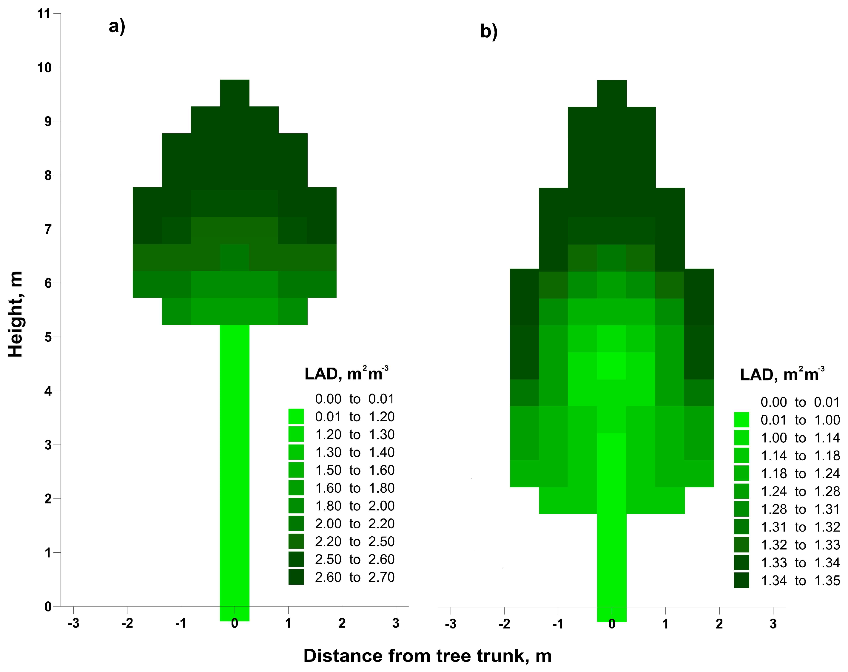
Appendix B. Parameterization of Tree Crown Structure

To create the appropriate crown shape, we used the following expression for functions R C ( z ) , specifying the crown radius at height z:
R C ( z ) = R max exp ( 1 2 k S ( z L T k M ( z 0 L T ) ) 2 )  
The functions describing leaves and branches distributions within the tree crown ( F l e a v e s ( R , z ) and F b r a n c h e s ( R , z ) , respectively) is expressed as:
F l e a v e s = k D { F s h a p e ( R , z ) ,        R T 2 R 2 R max ,    k M ( z 0 L T ) + L T z z 0 , F s h a p e ( R , z ) exp ( k L ( z L T k M ( z 0 L T ) ) ) ,      L T z k M ( z 0 L T ) + L T ,  
where F s h a p e = exp ( k U ( R 2 + ( z k C z 0 ) 2 R C 2 + ( z k C z 0 ) 2 ) 2 ) ,
F b r a n c h e s = { ( 1 R R max ) exp ( k S ( z L T k M ( z 0 L T ) ) 2 ) ,      k M ( z 0 L T ) + L T z z 0 , ( 1 R R max ) ,      L T z k M ( z 0 L T ) + L T ,  
Rmax is the maximal radius of tree crown for both tree species (assumed in our study to be equal 2 m), k D , k M , k S , k U , k L and k C are coefficients specifying structural properties of the trees of different species. The coefficient k D is the normalizing factor. Factor k M describes the location of the part of tree crown with the largest cross section, factor k S is a coefficient describing the outer shape of tree crown, and factors k U and k L are coefficients describing the leaf distribution in the upper and lower parts of tree crown, respectively. Factor k C describes the location of the tree crown part with maximal density of the leaves.
The model parameters for Silver birch have the following values: L T = 6   m , k D = 2.7 , k M = 1 / 3 , k S = k U = 20 , k L = 2 , and k C = 0.4 . Corresponding parameters for Scots pine are L T = 2   m , k D = 1.35 , k M = 1 / 3 , k S = k U = 5 , k L = 0.5 and k C = 0.5 .

References

  1. Ross, J. The Radiation Regime and Architecture of Plant Stands; Dr. W. Junk Publishers: The Hague, The Netherlands, 1981; 390p, ISBN-13 978-94-009-8649-7. [Google Scholar]
  2. Ruimy, A.; Jarvis, P.G.; Baldocchi, D.D.; Saugier, B. CO2 fluxes over plant canopies and solar radiation: A review. Adv. Ecol. Res. 1995, 26, 1–68. [Google Scholar] [CrossRef]
  3. Forster, P. Inference of climate sensitivity from analysis of earth’s energy budget. Annu. Rev. Earth Planet. Sci. 2016, 44, 85–106. [Google Scholar] [CrossRef]
  4. Armour, K. Energy budget constraints on climate sensitivity in light of inconstant climate feedbacks. Nat. Clim. Chang. 2017, 7, 331–335. [Google Scholar] [CrossRef]
  5. Nilson, T. Approximate analytical methods for calculating the reflection functions of leaf canopies in remote sensing applications. In Photon Vegetation Interactions. Applications in Optical Remote Sensing and Plant Ecology; Myneni, R., Ross, J., Eds.; Springer: Berlin/Heidelberg, Germany, 1991; pp. 161–190, ISBN-13 978-3-642-75391-6. [Google Scholar]
  6. Verstraete, M.M. Radiation transfer in plant canopies: Transmission of direct solar radiation and the role of leaf orientation. J. Geophys. Rev. 1987, 92, 10985–10995. [Google Scholar] [CrossRef]
  7. Myneni, R.; Ross, J.; Asrar, G. A review on the theory of photon transport in leaf canopies. Agric. For. Meteorol. 1989, 45, 1–153. [Google Scholar] [CrossRef]
  8. Knyazikhin, Y.; Marshak, A. Fundamental equations of radiative transfer in leaf canopies, and iterative methods of their solution. In Photon Vegetation Interactions. Applications in Optical Remote Sensing and Plant Ecology; Myneni, R., Ross, J., Eds.; Springer: Berlin/Heidelberg, Germany, 1991; pp. 9–43, ISBN-13 978-3-642-75391-6. [Google Scholar]
  9. Myneni, R.B. Modelling radiative transfer and photosynthesis in three dimensional vegetation canopies. Agric. For. Meteorol. 1991, 55, 323–344. [Google Scholar] [CrossRef]
  10. Kuusk, A. Canopy radiative transfer modeling. In Comprehensive Remote Sensing; Liang, S., Ed.; Terrestrial Ecosystems, Elsevier: Oxford, UK, 2018; Volume 3, pp. 9–22. ISBN 9780128032206. [Google Scholar]
  11. Kuusk, A.; Nilson, T. A directional multispectral forest reflectance model. Remote Sens. Environ. 2000, 72, 244–252. [Google Scholar] [CrossRef]
  12. Disney, M.; Lewis, P.; North, P. Monte Carlo ray tracing in optical canopy reflectance modelling. Remote Sens. Rev. 2000, 18, 163–196. [Google Scholar] [CrossRef]
  13. Kuusk, A. A two-layer canopy reflectance model. J. Quant. Spectrosc. Radiat. Transfer 2001, 71, 1–9. [Google Scholar] [CrossRef]
  14. Verhoef, W.; Bach, H. Simulation of hyperspectral and directional radiance images using coupled biophysical and atmospheric radiative transfer models. Remote Sens. Environ. 2003, 87, 23–41. [Google Scholar] [CrossRef]
  15. Pinty, B.; Lavergne, T.; Dickinson, R.; Widlowski, J.; Gobron, N.; Verstraete, M. Simplifying the interaction of land surfaces with radiation for relating remote sensing products to climate models. Atmospheres 2006, 111, D02116. [Google Scholar] [CrossRef]
  16. Widlowski, J.L.; Taberner, M.; Pinty, B.; Bruniquel-Pinel, V.; Disney, M.; Fernandes, R.; Gastellu-Etchegorry, J.P.; Gobron, N.; Kuusk, A.; Lavergne, T.; et al. Third radiation transfer model intercomparison (RAMI) exercise: Documenting progress in canopy reflectance models. Atmospheres 2007, 112, D09111. [Google Scholar] [CrossRef]
  17. Widlowski, J.L.; Pinty, B.; Clerici, M.; Dai, Y.; De Kauwe, M.; de Ridder, K.; Kallel, A.; Kobayashi, H.; Lavergne, T.; Ni-Meister, W.; Olchev, A.; et al. RAMI4PILPS. An Intercomparison of Formulations for the Partitioning of Solar Radiation in Land Surface Models. Geophys. Res. 2011, 116, G02019. [Google Scholar] [CrossRef]
  18. Meador, W.E.; Weaver, W.R. Two-stream approximations to radiative transfer in planetary atmospheres: A unified description of existing methods and a new improvement. J. Atmos. Sci. 1980, 37, 630–643. [Google Scholar] [CrossRef]
  19. Dickinson, R.E. Land surface processes and climate-surface albedos and energy balance. Adv. Geophys. 1983, 25, 305–353. [Google Scholar] [CrossRef]
  20. Goel, N. Models of vegetation canopy reflectance and their use in estimation of biophysical parameters from reflectance data. Remote Sens. Rev. 1988, 4, 1–212. [Google Scholar] [CrossRef]
  21. Knyazikhin, Yu.; Kranigk, J.; Miessen, G.; Panfyorov, O.; Vygodskaya, N.; Gravenhorst, G. Modelling three-dimensional distribution of photosynthetically active radiation in sloping coniferous stands. Biomass Bioenergy 1996, 11, 189–200. [Google Scholar] [CrossRef]
  22. Knyazikhin, Yu.; Miessen, G.; Panfyorov, O.; Gravenhorst, G. Small-scale study of three-dimensional distribution of photosynthetically active radiation in a forest. Agric. For. Meteorol. 1997, 88, 215–239. [Google Scholar] [CrossRef]
  23. Gravenhorst, G.; Knyazikhin, Yu.; Kranigk, J.; Mießen, G.; Panfyorov, O.; Schnitzler, K.G. Is forest albedo measured correctly? Meteorol. Z. 1999, 8, 107–114. [Google Scholar] [CrossRef]
  24. Pinty, B.; Gobron, N.; Widlowski, J.L.; Gerstl, S.A.; Verstraete, M.M.; Antunes, M.; Bacour, C.; Gaston, F.; Gastellu, J.P.; Goel, N.; et al. Radiation transfer model intercomparison (RAMI) exercise. Atmospheres 2001, 106, 11937–11956. [Google Scholar] [CrossRef] [Green Version]
  25. Asrar, G. and Myneni, R.B. Applications of Radiative Transfer Models for Remote Sensing of Vegetation Conditions and States. In Photon-Vegetation Interactions: Applications in Optical Remote Sensing and Plant Physiology; Myneni, R.B., Ross, J., Eds.; Springer: Berlin & Heidelberg, Germany, 1991; pp. 539–557. [Google Scholar]
  26. Nilson, T.; Ross, J. Modeling radiative transfer through forest canopies: Implications for canopy photosynthesis and remote sensing. In The Use of Remote Sensing in the Modeling of Forest Productivity; Gholz, H., Nakane, K., Shimoda, H., Eds.; Kluwer: Dordrecht, The Netherlands, 1997; pp. 23–60. ISBN 978-94-010-6290-9. [Google Scholar]
  27. Marshak, A.; Knyazikhin, Y. The spectral invariant approximation within canopy radiative transfer to support the use of the EPIC/DSCOVR oxygen B-band for monitoring vegetation. J. Quant. Spectrosc. Radiat. Trans. 2017, 191, 7–12. [Google Scholar] [CrossRef] [PubMed] [Green Version]
  28. Yang, B.; Knyazikhin, Y.; Mõttus, M.; Rautiainen, M.; Stenberg, P.; Yan, L.; Chen, C.; Yan, K.; Choi, S.; Park, T.; Myneni, R.B. Estimation of leaf area index and its sunlit portion from DSCOVR EPIC data: Theoretical basis. Remote Sens. Environ. 2017, 198, 69–84. [Google Scholar] [CrossRef] [PubMed] [Green Version]
  29. Li, W.; Ciais, P.; Wang, Y.; Yin, Y.; Peng, S.; Zhu, Z.; Bastos, A.; Yue, C.; Ballantyne, A.P.; Broquet, G. Recent Changes in Global Photosynthesis and Terrestrial Ecosystem Respiration Constrained from Multiple Observations. Geophys. Res. Lett. 2018, 45, 1058–1068. [Google Scholar] [CrossRef]
  30. Myneni, R.B.; Asrar, G.; Gerstl, S.A.W. Radiative transfer in three dimensional leaf canopies. Transp. Theory Stat. Phys. 1990, 19, 205–250. [Google Scholar] [CrossRef]
  31. Knyazikhin, Y.; Marshak, A.; Myneni, R.B. Three dimensional radiative transfer in vegetation canopies. In Three Dimensional Radiative Transfer in the Cloudy Atmosphere; Marshak, A., Davis, A.B., Eds.; Springer: Berlin/Heidelberg, Germany, 2005; pp. 617–652. ISBN 978-3-540-23958-1. [Google Scholar]
  32. Lukeš, P.; Stenberg, P.; Rautiainen, M.; Mõttus, M.; Vanhatalo, K.M. Optical properties of leaves and needles for boreal tree species in Europe. Remote Sens. Lett. 2013, 4, 667–676. [Google Scholar] [CrossRef]
  33. Abakumova, M.; Gorbarenko, E.V.; Nezval, E.I.; Shilovzeva, O.A. Climatological Resources of Solar Energy in Moscow Region; Librocom: Moscow, Russia, 2012; 310p. (In Russian) [Google Scholar]
  34. Myneni, R.B.; Marshak, A.; Knyazikhin, Y.; Asrar, G. Discrete Ordinates Method for Photon Transport in Leaf Canopies. In Photon Vegetation Interactions. Applications in Optical Remote Sensing and Plant Ecology; Myneni, R., Ross, J., Eds.; Springer: Berlin/Heidelberg, Germany, 1991; pp. 45–106, ISBN-13 978-3-642-75391-6. [Google Scholar]
  35. Lebedev, V.I. Values of the nodes and weights of ninth to seventeenth order Gauss-Markov quadrature formulae invariant under the octahedron group with inversion. USSR Comput. Math. Math. Phys. 1975, 15, 44–51. [Google Scholar] [CrossRef]
  36. Tikhonov, A.N.; Goncharsky, A.V.; Stepanov, V.V.; Yagola, A.G. Numerical Methods for the Solution of Ill-Posed Problems; Kluwer Academic Publishers: Dordrecht, The Netherlands, 1995; p. 253. ISBN 0-7923-3583-X. [Google Scholar]
  37. Ruimy, A.; Dedieu, G.; Saugier, B. TURC: A diagnostic model of continental gross primary productivity and net primary productivity. Global Biogeochem. Cycles 1996, 10, 269–285. [Google Scholar] [CrossRef]
  38. Running, S.W.; Nemani, R.R.; Heinsch, F.A.; Zhao, M.; Reeves, M.; Hashimoto, H. A continuous satellite derived measure of global terrestrial primary production. BioScience 2004, 54, 547–560. [Google Scholar] [CrossRef]
  39. Xiao, X.; Hollinger, D.; Aber, J.; Goltz, M.; Davidson, E.; Zhang, Q.; Moore, B. Satellite-based modeling of gross primary production in an evergreen needleleaf forest. Remote Sens. Environ. 2004, 89, 519–534. [Google Scholar] [CrossRef]
  40. Ibrom, A.; Oltchev, A.; June, T.; Kreilein, H.; Rakkibu, G.; Ross, T.H.; Panferov, O.; Gravenhorst, G. Variation in photosynthetic light-use efficiency in a mountainous tropical rain forest in Indonesia. Tree Physiol. 2008, 28, 499–508. [Google Scholar] [CrossRef] [PubMed] [Green Version]
  41. Pinker, R.T.; Thompson, O.E.; Eck, T.F. The albedo of a tropical evergreen forest. Q. J. R. Meteorol. Soc. 1980, 106, 551–558. [Google Scholar] [CrossRef]
  42. Giambelluca, T.W.; Hölscher, D.; Bastos, T.X.; Frazão, R.R.; Nullet, M.A.; Ziegler, A.D. Observations of albedo and radiation balance over postforest land surfaces in the eastern Amazon basin. J. Clim. 1997, 10, 919–928. [Google Scholar] [CrossRef]
  43. Kimes, D.S.; Sellers, P.J.; Newcomb, W.W. Hemispherical reflectance variations of vegetation canopies and implications for global and regional energy budget studies. J. Clim. Appl. Meteorol. 1987, 26, 959–972. [Google Scholar] [CrossRef]
  44. Grant, I.F.; Prata, A.J.; Cechet, R.P. Diurnal Variation of Albedo on the Remote Sensing of the Daily Mean Albedo of Grassland. J. Clim. Appl. Meteorol. 2000, 39, 231–244. [Google Scholar] [CrossRef]
  45. Simioni, G.; Durand-Gillmann, M.; Huc, R. Asymmetric competition increases leaf inclination effect on light absorption in mixed canopies. Ann. For. Sci. 2013, 70, 123–131. [Google Scholar] [CrossRef]
  46. Kranigk, J.; Gruber, F.; Heimann, J.; Thorwest, A. Ein Model für die Kronenraumstruktur und die räumliche Verteilung der Nadeloberflache in einem Fichtenbestand. Allg. For. Jagdztg. 1994, 165, 193–197. [Google Scholar]
  47. Knyazikhin, Y.; Martonchik, S.W.; Myneni, R.B.; Diner, D.J.; Running, S.W. Synergistic algorithm for estimating vegetation canopy leaf area index and fraction of absorbed photosynthetically active radiation from MODIS and MISR data. J. Geophys. Res. 1998, 103, 32257–32276. [Google Scholar] [CrossRef]
  48. Kimes, D.S.; Knyazikhin, Y.; Privette, J.L.; Abuelgasim, A.A.; Gao, F. Inversion methods for physically-based models. Remote Sens. Rev. 2000, 18, 381–439. [Google Scholar] [CrossRef]
  49. Ni, X.; Zhou, Y.; Cao, C.; Wang, X.; Shi, Y.; Park, T.; Choi, S.; Myneni, R.B. Mapping Forest Canopy Height over Continental China Using Multi-Source Remote Sensing Data. Remote Sens. 2015, 7, 8436–8452. [Google Scholar] [CrossRef] [Green Version]
  50. Schneider, F.D.; Morsdorf, F.; Schmid, B.; Petchey, O.L.; Hueni, A.; Schimel, D.S.; Schaepman, M.E. Mapping functional diversity from remotely sensed morphological and physiological forest traits. Nat. Commun. 2017, 8, 1441. [Google Scholar] [CrossRef] [PubMed] [Green Version]
  51. Shen, X.; Cao, L. Tree-species classification in subtropical forests using airborne hyperspectral and LiDAR data. Remote Sens. 2017, 9, 1180. [Google Scholar] [CrossRef]
  52. Martin, M.E.; Newman, S.D.; Aber, J.D.; Congalton, R.G. Determining forest species composition using high spectral resolution remote sensing data. Remote Sens. Environ. 1998, 65, 249–254. [Google Scholar] [CrossRef]
  53. Waser, L.T.; Küchler, M.; Jütte, K.; Stampfer, T. Evaluating the potential of WorldView-2 data to classify tree species and different levels of ash mortality. Remote Sens. 2014, 6, 4515–4545. [Google Scholar] [CrossRef]
  54. Zhang, Y.; Lukyanenko, D.V.; Yagola, A.G. Using Lagrange principle for solving linear ill-posed problems with a priori information. Numer. Methods Program. 2013, 14, 468–482. (In Russian) [Google Scholar]
  55. Wang, Y.F.; Zhang, Y.; Lukyanenko, D.V.; Yagola, A.G. Recovering aerosol particle size distribution function on the set of bounded piecewise-convex functions. Inverse Probl. Sci. Eng. 2013, 21, 339–354. [Google Scholar] [CrossRef]
  56. Zhang, Y.; Lukyanenko, D.V.; Yagola, A.G. An optimal regularization method for convolution equations on the source wise represented set. J. Inverse Ill-Posed Probl. 2015, 23, 465–476. [Google Scholar] [CrossRef]
Figure 1. The arrangement of the ray reflected from point r M and captured by the sensor located at some height h above point r.
Remotesensing 10 01661 g001
Figure 2. The spatial distributions of birch and pine leaf area index (LAI) within the modeling domain for a scenario, assuming the same proportion of both tree species within the forest stand. Birch and pine trees are shown by green and yellow colors, respectively.
Remotesensing 10 01661 g002
Figure 3. A schematic representation of the spatial distribution of photosynthesizing and non-photosynthesizing phytomass for (a) Silver birch and (b) Scots pine. Leaf area density (LAD) for Silver birch varied between 0.65 and 2.7 m2 m−2 and for Scots pine between 0.65 and 1.4 m2 m−2.
Remotesensing 10 01661 g003
Figure 4. Location and sequence of the calculated elements of the grid: (a) I octant, (b) II octant, (c) III octant, (d) IV octant, (e) V octant, (f) VI octant, (g) VII octant, and (h)VIII octant.
Remotesensing 10 01661 g004
Figure 5. The modeling domain D for which the model functions ρ 1 ( x , y ) and ρ 2 ( x , y ) were reconstructed. It was assumed that deciduous and coniferous tree species were uniformly distributed within the modeling domain. Dashes indicate the grid cells for which the ratio of different tree species was retrieved.
Remotesensing 10 01661 g005
Figure 6. Smoothed spatial patterns of tree density distribution ρ 1 ( x , y ) (a) and ρ 2 ( x , y ) (b) of deciduous and coniferous tree species within the modeling domain D { ( x , y ) : 50 x 50 , 50 y 50 } .
Remotesensing 10 01661 g006
Figure 7. Dependence of canopy albedo on sun elevation and the fraction of deciduous and coniferous tree species in a mixed forest stand of different stock densities (LAI = 1 and 4 m2 m−2). All modeling experiments were completed for dark (ρs = 0.01) and light (ρs = 0.20) soils.
Remotesensing 10 01661 g007
Figure 8. The result of the functions ρ 1 ( x , y ) (a) and ρ 2 ( x , y ) (b) retrieving on the N x × N y 100 × 80 grids for a set of measurements of N p = 10 points with simulated errors h = 1%, δ = 1 % .
Remotesensing 10 01661 g008
Figure 9. The result of the functions ρ 1 ( x , y ) (a) and ρ 2 ( x , y ) (b) retrieving on the N x × N y 100 × 80 grids for a set of measurements of N p = 10 points with simulated errors δ = 5 % , h = 6 % .
Remotesensing 10 01661 g009
Figure 10. The result of the functions ρ 1 ( x , y ) (a) and ρ 2 ( x , y ) (b) retrieving on the N x × N y 100 × 80 grids for a set of measurements of N p = 500 points with simulated errors δ = 5 % , h = 6 % .
Remotesensing 10 01661 g010
Figure 11. The root-mean-square errors s in the components of reconstructed vector X i n v of the error levels δ in the input data and the model error h for the fixed number of measurement points N p = 10 (a) and N p = 500 (b).
Remotesensing 10 01661 g011
Figure 12. Graph of the root-mean-square error s in the components of the reconstructed vector X i n v of the number of measurement points N p (for a fixed error levels δ in the input data and h in the model).
Remotesensing 10 01661 g012

