Article

Application and Validation of a Model for Terrain Slope Estimation Using Space-Borne LiDAR Waveform Data

1
Key Laboratory of Digital Earth Science, Institute of Remote Sensing and Digital Earth, Chinese Academy of Sciences, Beijing 100094, China
2
University of Chinese Academy of Sciences, Beijing 100049, China
3
Beijing Institute of Spacecraft System Engineering, Beijing 100094, China
*
Author to whom correspondence should be addressed.
Remote Sens. 2018, 10(11), 1691; https://0-doi-org.brum.beds.ac.uk/10.3390/rs10111691
Submission received: 3 August 2018 / Revised: 15 October 2018 / Accepted: 24 October 2018 / Published: 26 October 2018

Abstract

:
The terrain slope is one of the most important surface characteristics for quantifying the Earth surface processes. Space-borne LiDAR sensors have produced high-accuracy and large-area terrain measurement within the footprint. However, rigorous procedures are required to accurately estimate the terrain slope especially within the large footprint since the estimated slope is likely affected by footprint size, shape, orientation, and terrain aspect. Therefore, based on multiple available datasets, we explored the performance of a proposed terrain slope estimation model over several study sites and various footprint shapes. The terrain slopes were derived from the ICESAT/GLAS waveform data by the proposed method and five other methods in this study. Compared with five other methods, the proposed method considered the influence of footprint shape, orientation, and terrain aspect on the terrain slope estimation. Validation against the airborne LiDAR measurements showed that the proposed method performed better than five other methods (R2 = 0.829, increased by ~0.07, RMSE = 3.596°, reduced by ~0.6°, n = 858). In addition, more statistics indicated that the proposed method significantly improved the terrain slope estimation accuracy in high-relief region (RMSE = 5.180°, reduced by ~1.8°, n = 218) or in the footprint with a great eccentricity (RMSE = 3.421°, reduced by ~1.1°, n = 313). Therefore, from these experiments, we concluded that this terrain slope estimation approach was beneficial for different terrains and various footprint shapes in practice and the improvement of estimated accuracy was distinctly related with the terrain slope and footprint eccentricity.

1. Introduction

The Earth surface survey provides fundamental and useful geo-information for terrestrial ecosystems, global climate monitoring, and landform mapping [1,2,3,4]. We extremely focus on quantifying Earth’s surface characteristics (e.g., elevation, slope, and aspect) because these characteristics provide valid indicators for the climate, precipitation, and ocean currents [5,6,7]. However, it is still a major challenge to monitor the surface topography consecutively and accurately over large areas. Development of space-borne remote sensing techniques has addressed this challenge to some extent [8,9,10]. For instance, the optical stereo photogrammetry and Synthetic Aperture Radar have generated the available global digital elevation models (DEMs) [10,11]. However, complex matching operations must be done to produce DEMs from stereos and the optical images are susceptible to the weather. Moreover, the vertical accuracies of these DEMs are not high at ~15 m [12,13,14]. In contrast, LiDAR sensors can directly acquire the surface height information by measuring the time of the transmitted and received pulses [15,16]. Its high-frequency sampling makes great promises of high vertical accuracy [17,18,19,20,21,22]. Therefore, the space-borne LiDAR has become the most promising technique for accurately measuring the terrain characteristics on a global scale [21,22].
Ice, Cloud, and land Elevation Satellite (ICESat)/Geoscience Laser Altimeter System (GLAS) is the first space-borne LiDAR mission of recording global full-waveform altimetry data within the footprint [21,23]. Effective global or region GLAS products have been applied to measure the land topography and ice sheet mass balance [24,25,26]. Terrain slope is one of the most important surface characteristics. Some previous studies have also emphasized the significance of the terrain slope estimation. For instance, the within-footprint terrain slope has an obvious impact on most waveform characteristics because its broadening effect mixes the object return and the ground return [27,28,29].
To more accurately estimate the within-footprint terrain slope and to understand the complex relation between waveform characterization and surface terrain, several proposed physical models and methods have achieved the terrain slope estimation by using the full-waveform LiDAR data [30,31,32]. Among these methods, most have been built by simplifying the footprint shape into a circle [30,31]. They ignored the fact that the true footprint shape was closer to be elliptical rather than circular [29,33,34]. In contrast, this phenomenon was taken into accounts in the study of Nie et al. [32]. They quantified the influence of footprint size, shape, orientation, and terrain aspect on terrain slope estimation by a series of theoretical physically-based analyses. A subsequent slope estimation model was proposed to reduce the impact of these various factors. This estimation approach has been proven to be theoretically feasible on estimating the terrain slope within the footprint more accurately, but it still needs to be applied and validated on a large area with a different terrain and various LiDAR footprints.
Therefore, the primary goal in this study is to practice the terrain slope estimation model of Nie et al. [32] over several study sites based on GLAS data. We validated the GLAS-estimated slopes (by the proposed method considering footprint shape, orientation, and terrain aspect and five other methods without considering them) with respect to comparisons against the airborne LiDAR data. After demonstrating the efficacy of the terrain slope estimation approach, we attempted to analyze the effects of different factors (e.g., terrain slope, footprint size, and eccentricity) on the terrain slope estimation by relating these factors to the actual absolute errors. The accuracy improvement and applicability of these terrain slope estimation methods were simply investigated based on the comparison results in different terrain and various footprint shapes. In addition, some other error sources (e.g., terrain condition and surface covering condition) were also analyzed in this work.

2. Materials

2.1. Study Area

We selected four study sites where all used datasets were available for the terrain slope estimation. Two sites are located in Greenland and the other two are located in Antarctica. These areas are barely covered by snow and vegetation. Temporal variations in topography in these areas are relatively small. The sites covered different topographies ranging from flat to high relief. Some characteristics of four study sites were summarized in Table 1. Geographical locations and topographic information were shown in Figure 1.

2.2. GLAS Data

GLAS is the first space-borne laser altimeter for Earth observation, which was launched by the National Aeronautics and Space Administration (NASA) in 2003. It emitted a temporal Gaussian laser pulse for a duration of approximately 4 to 6-ns FWHM (full width half maximum) [35]. Return signals were recorded in the form of a continuous waveform reflecting multiple information (e.g., height, density, and reflectivity) of the intercepted surfaces [35,36]. The emitted laser pulses took shape of the footprints with around a 70-m diameter and a 170-m center-to-center spacing. The horizontal position accuracy of footprints is about 4.8 m and the vertical accuracy is 13.8 cm [37].
National Snow and Ice Data Center (NSIDC) provides 15 types of GLAS product (GLA01~GLA15) [38] of which GLA01, GLA05, and GLA12 were used in this study. The GLA01 product records the raw full-waveform data including the transmitted and received waveform. The GLA05 product provides the detailed description of footprint size, shape, and orientation. The GLA12 product is used to obtain laser spot geo-location and surface elevation. Table 2 summarized the parameters of GLA01, GLA05, and GLA12 used in the terrain slope estimation. In this study, the GLAS datasets of Greenland sites were from Laser 3I in October 2007 and the datasets of Antarctica were from Laser 3K in October 2008. Each GLAS footprint is a variable ellipse with a slightly different orientation, size, and eccentricity. The average footprint sizes (minor and major axes) are 46 m × 57 m for 3I campaign and 41 m × 52 m for 3K campaign.
We screened the GLAS data to obtain a high-quality dataset and ensure the validity of the experiments. Invalid GLAS data without geographical coordinates or affected by clouds (the flag i_FRir_qaFlag ≠ 15 in the GLA12 product) was removed [31,33].

2.3. ASTER GDEM Data

ASTER GDEM (Advanced Space-borne Thermal Emission and Reflection Radiometer Global Digital Elevation Model) was used to calculate the prior terrain aspect, which was combined with the footprint orientation to flexibly choose the terrain slope estimation method. ASTER, which is onboard with the NASA Terra, collected the in-track stereos using nadir-looking and aft-looking near infrared cameras [39,40]. These stereos were used to produce the global digital elevation model. The GDEM data is available from 83° S to 83° N and covers most of the polar region [41]. We used Version 2 of GDEM in this study [42]. Although changes in the stereo processing have produced significant improvements in GDEM2 as compared to GDEM1, the validated horizontal accuracy of GDEM2 is still ~30 m and the vertical accuracy is ~20 m [43,44,45]. Therefore, in order to avoid introducing a new error source, the terrain aspect calculated from GDEM2 was only used as an auxiliary parameter but not an input parameter of the estimation method.
The terrain aspect was calculated as the direction of the maximum rate of change in the elevation of GDEM. The extraction of the terrain aspect was conducted by using the mapping and analytics software ArcGIS 10.2.

2.4. ATM Data

Airborne Topographic Mapper (ATM) data was used to verify the accuracy of the terrain slope estimation method in this study. It was developed by NASA to observe the Earth’s topography and, most importantly, to measure the changes of ice sheets and glaciers in North America, Greenland, and Antarctica [46,47,48]. The L1B ATM data records the spot elevation and return strength measurements over the sea ice and ice sheet surfaces where the vertical accuracy is 6.6 cm [49]. The L2 data comprises the elevation, slope, and roughness datasets that were calculated from L1B data. The Preicebridge ATM data was utilized in this paper because of the close collected times with other datasets. The acquisition dates of the ATM data, GLAS data, and ASTER GDEM are almost identical (Table 3).

3. Methods

3.1. Terrain Slope Estimation Method

Below, we gave an outline of the terrain slope estimation method (referred to as the flexible method) and tested it on the GLAS waveform across four study sites.
The within-footprint terrain slope can be quantitatively inversed by the ground vertical extent and footprint diameter, which is shown in Equation (1). Five different footprint diameters were adopted for calculating the terrain slope (Equations (2)–(6)). They are the semi-major axis a, the semi-minor axis b, the arithmetic mean, the quadratic mean, and the geometrical mean of a and b. A series of theoretical analyses [32] indicated that the terrain slope error estimated by these five diameters varied regularly with the intersection angle between the footprint orientation and terrain aspect (Figure 2). Every diameter was found to be optimal only for environments with some range of intersection angles. Therefore, we chose the flexible slope estimation method based on the intersection angle once the four threshold values ( θ 1 , θ 2 , θ 3 , θ 4 in Figure 2) were obtained, which is shown in Equation (7).
η = atan ( h d )
Method   1 :   η 1 = atan ( h 2 a )
Method   2 :   η 2 = atan ( h 2 b )
Method   3 :   η 3 = atan ( h a + b )
Method   4 :   η 4 = atan ( h 2 a b )
Method   5 :   η 5 = atan ( h 2 a 2 + b 2 2 )
Flexible   Method :   η = { η 1 ,   if   0 θ < θ 1   or   π θ 1 θ < π η 2 ,   if   θ 4 θ < π θ 4 η 3 ,   if   θ 2 θ < θ 3   or   π θ 3 θ < π θ 2 η 4 ,   if   θ 3 θ < θ 4   or   π θ 4 θ < π θ 3 η 5 ,   if   θ 1 θ < θ 2   or   π θ 2 θ < π θ 1
where h is the ground vertical extent, d is the footprint diameter, η is the estimated terrain slope, θ is the intersection angle between the terrain aspect and footprint orientation, and a and b are the semi-major and semi-minor axes of each footprint, respectively.
The four threshold values of the intersection angle used for choosing the estimation method can be calculated by Equations (8)–(11). The left and right sides of each equation represented the theoretical absolute errors by two methods of the left and right sides of the threshold value in Figure 2, respectively.
θ 1 :   atan ( h 2 a ) - atan ( h 2 a 2 cos 2 ( θ 1 ) + b 2 sin 2 ( θ 1 ) ) = atan ( h 2 a 2 cos 2 ( θ 1 ) + b 2 sin 2 ( θ 1 ) ) - atan ( h 2 a 2 + b 2 2 )
θ 2 :   atan ( h 2 a ) - atan ( h 2 a 2 cos 2 ( θ 2 ) + b 2 sin 2 ( θ 2 ) ) = atan ( h 2 a 2 cos 2 ( θ 2 ) + b 2 sin 2 ( θ 2 ) ) - atan ( h 2 a 2 + b 2 2 )
θ 3 :   atan ( h a + b ) - atan ( h 2 a 2 cos 2 ( θ 3 ) + b 2 sin 2 ( θ 3 ) ) = atan ( h 2 a 2 cos 2 ( θ 3 ) + b 2 sin 2 ( θ 3 ) ) - atan ( h 2 a b )
θ 4 :   atan ( h 2 a b ) - atan ( h 2 a 2 cos 2 ( θ 4 ) + b 2 sin 2 ( θ 4 ) ) = atan ( h 2 a 2 cos 2 ( θ 4 ) + b 2 sin 2 ( θ 4 ) ) - atan ( h 2 b )
In general, the flexible terrain slope estimation contained two steps, which includes the calculation of ground extent and the choice of the footprint diameter. Based on these two steps, we estimated the terrain slope by the flexible method, validated the estimated accuracy, and analyzed the terrain slope errors. Our detailed scheme was shown in Figure 3.

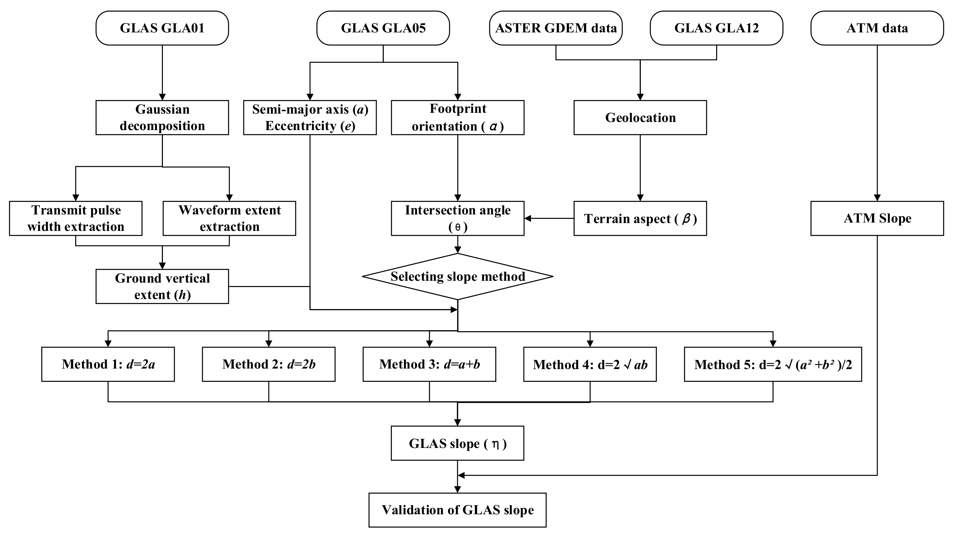
3.1.1. Calculation of Ground Extent

Ground extent (h) represents the ground vertical height within the footprint, which can be calculated from waveform analysis [29,50,51,52]. The effect of the terrain slope on the waveform extent for the nadir-pointing laser can be expressed in Figure 4a–c. It is obvious that the ground return was stretched by introducing the terrain slope within the footprint. Therefore, the ground extent can be extracted based on the decomposed ground waveform metrics from GLAS in this study [51,52].
First, the original GLAS waveform was smoothed by using a moving mean filter to eliminate the noise signal. Then Gaussian decomposition was used to decompose the de-noised waveform into a series of Gaussian peaks [53,54]. The last decomposed waveform was considered as the ground waveform [55,56]. After obtaining the ground waveform, we extracted the ground signal beginning location and end location above 4.5 times the noise standard deviation to obtain the ground waveform extent (Figure 4d). Lastly, the ground extent was calculated from the ground waveform extent by eliminating the broadening effect of the emitted laser pulse, which is shown in Equation (12).
h = G r o u n d   W a v e f o r m   E x t e n t c F W H M
where c is the light velocity and FWHM is the full width half maximum of the emitted pulse width.

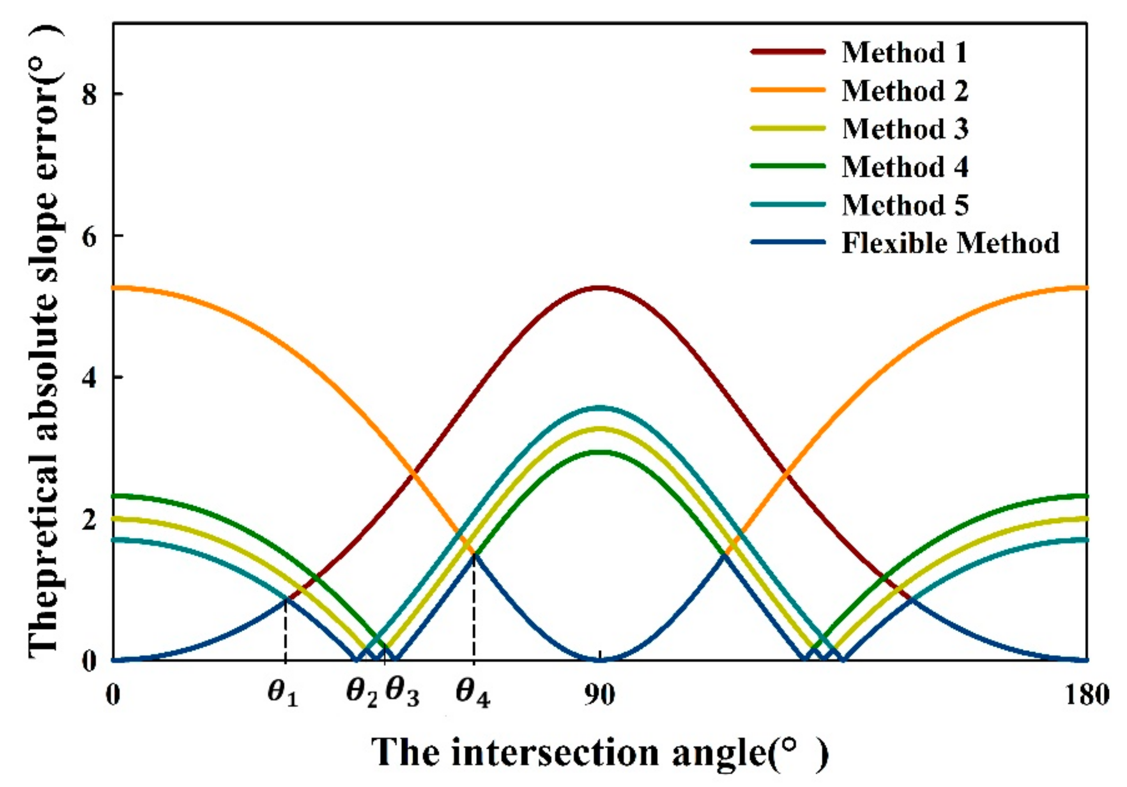
3.1.2. Choice of Footprint Diameter

The chosen footprint diameter determines the estimation accuracy of the terrain slope. From Figure 4e, the effective footprint diameter (d) is related to the intersection angle between the terrain aspect and footprint orientation.
Five estimation methods (Equations (2)–(6)) using a certain value to represent the footprint diameter do not consider the coupling effect of the footprint shape, orientation, and the terrain aspect. In contrast, the flexible method chooses the most appropriate footprint diameter on the terrain slope estimation.
Hence, we obtained the intersection angle as the difference of the terrain aspect from ASTER GDEM2 and the footprint orientation from GLAS data. Afterward, four threshold values were calculated by substituting the footprint major axis, minor axis, and ground extent into Equations (8)–(11). The optimal footprint diameter was determined by comparing the intersection angle with four threshold angles. Lastly, the terrain slope was calculated from the ground extent divided by the chosen footprint diameter.

3.2. Validation and Analysis of the Terrain Slope Derived from GLAS

We explored the terrain slope estimation approach by GLAS data across different sites. The terrain slopes retrieved from GLAS were validated by the ATM-observed slopes. The estimation accuracy was evaluated based on the error bias, standard deviation, the root-mean-square error (RMSE), and the coefficient of determination (R2). More error analyses were done by visualizing and fitting the distribution of the slope errors. In addition, the results of the flexible method were compared with those estimated by five other slope estimation methods with the same datasets. To further evaluate the performance of the flexible method, we also compared the estimation accuracy of the flexible method and five direct methods in different terrains and various eccentricity footprints.

4. Results and Discussion

4.1. Validation Against Airborne LiDAR Slope

We compared the GLAS-derived terrain slope with the ATM-measured slope for all sites by the flexible method and five direct methods. The results were summarized in Figure 5 and Table 4. Overall, the terrain slopes derived from the six methods all had moderately linear correlations with the ATM-observed terrain slopes. However, compared to the five other methods, the flexible method had a lower standard deviation (3.592°), lower RMSE (3.596°), and higher R2 (0.829) in the terrain slope estimation. This indicated that the estimation of the terrain slope was improved by considering the footprint shape, orientation, and terrain aspect.
For method 1, the regression result was slightly on the left side of the 1:1 line. The estimated bias error (−0.556) also showed that choosing the major axis as the footprint diameter led to the underestimation of the terrain slope. In contrast, the regression result and bias error of method 2 represented that choosing the minor axis led to the overestimation of the terrain slope. The regression lines of methods 3, 4, 5, and the flexible method almost coincided with the 1:1 line. We also found that methods 3, 4, and 5 had slightly lower RMSE and higher R2 when compared with methods 1 and 2. This indicated that choosing the value between the major and minor axes achieved slightly higher accuracy. At the same time, they corrected the underestimation of method 1 and the overestimation of method 2 to some degree.
Upon further analysis of the terrain errors of these methods, we visualized the estimated errors in the histograms and fitted them by the normal distribution curves. Relevant results were shown in Figure 6 and Figure 7. Although the errors of all methods followed the normal distribution, the means and variances of the distribution curves tell us more. The mean of error by method 1 is less than zero, by method 2 is more than zero, and, by other methods, are very close to zero. The underestimation of method 1 and the overestimation of method 2 were more clearly shown in Figure 7. However, although methods 3, 4, and 5 reduced the underestimation and overestimation of method 1 and 2, the variances hardly decreased. The flexible method not only corrected the under-or-over estimation but also made the errors more concentrated and closer to zero. These results verified the conclusions in Figure 5 and Table 4 from the perspective of the error distribution.
Although the flexible method had much higher estimation accuracy in terms of R2, the RMSE of the terrain slope only improved by ~0.5° when compared with the five other methods (Table 4). This may be due to a mass of points in the low-relief region. For these points, whichever one chosen as the footprint diameter made little difference in the absolute errors of the terrain slope estimates. Thus, the estimation accuracy of the terrain slope was slightly better when using the flexible method.

4.2. Slope Estimation of Different Terrain Relief

Figure 8 showed the absolute mean difference between the ATM-observed and the GLAS-predicted terrain slopes with the gradient of the terrain slope, which also supported the conclusion that the flexible method was superior to five other methods in estimating the within-footprint terrain slope. Among the five direct methods, method 2 usually has the largest estimation error, which is followed by method 1. The estimation errors of methods 3, 4, and 5 are close with all of them being less than methods 1 and 2. This coincided with the theoretical error analyzed by Reference [32]. In addition, we also found that, as the terrain slope observed from ATM increased, the absolute mean error was reduced more by the flexible method. For instance, when the terrain slope is less than 5°, the curves of six methods in Figure 8 were almost identical. With the increment of the terrain slope, the difference between the curve of the flexible method and other curves increased. Therefore, we made quantitative statistics of 218 GLAS footprints in the high-relief region (slope observed by ATM > 5°) and 640 footprints in the low-relief region (slope observed by ATM ≤ 5°). The results of slope estimation in the high-relief and low-relief regions were summarized in Table 5.
The results in the high-relief region (n = 218, R2 = 0.757, RMSE = 5.180°) and in the low-relief region (n = 640, R2 = 0.636, RMSE = 0.936°) yielded the similar conclusions as the results of all data. In addition, the flexible method significantly reduced the RMSE of the terrain slope estimation by ~1.4° when compared with methods 3, 4, and 5 and by ~1.8° when compared with methods 1 and 2 in the high-relief region. The detailed results in the high-relief region were clearly shown in Figure 9. Conversely, in the low-relief region, the RMSE of the flexible method was only reduced by ~0.1°. In theory, the coupling effect of the footprint orientation and terrain aspect will lead to the greater absolute error when the terrain slope is greater [32]. The flexible method significantly reduced this absolute error in the high-relief region both theoretically and practically. Therefore, we would use the flexible method to estimate the within-footprint terrain slope in the high-relief region.

4.3. Slope Estimation of Different Footprint Eccentricity

Figure 10 showed the absolute mean error of GLAS-derived terrain slopes with the gradient of footprint eccentricity. Overall, the terrain slope errors by all methods increased with the ellipse eccentricity. This coincided with the theoretical error analyses of footprint eccentricity [32]. Beyond that, as the footprint eccentricity increased, the flexible method decreased more error of the terrain slope. Hence, we did the statistics of 313 GLAS footprints whose ellipse eccentricity was greater than 0.6 and 545 GLAS footprints with eccentricity less than 0.6. The results of the slope estimations with different footprint eccentricity were summarized in Table 6.
From Table 6, the flexible method performed better for datasets with high-eccentricity footprints (n = 313, R2 = 0.838, RMSE = 3.421°) compared with the footprints with low eccentricity (n = 545, R2 = 0.813, RMSE = 3.596°). For the high-eccentricity footprints, the flexible method significantly reduced the RMSE of the terrain slope estimation by ~0.8° when compared with methods 3, 4, and 5 and by ~1.1° compared with methods 1 and 2. The RMSE of low-eccentricity footprints was only reduced by ~0.4° when compared with other methods. Figure 11 showed the detailed validation results for the dataset whose eccentricity was greater than 0.6. This verified the theoretical error analysis in Reference [32]. When the footprint eccentricity is small, there is little difference among several adopted footprint diameters. The terrain slope error is theoretically small. However, in cases of the greater eccentricity, the coupling effect of the footprint shape, orientation, and terrain aspect must be fully considered on the terrain slope estimation.

4.4. Slope Estimation of Different Footprint Size

Figure 12 showed the absolute mean error of GLAS-derived terrain slopes as a function of the footprint diameter gradients. The footprint diameters of the dataset used in this study were approximately 48 m to 63 m. In theory, the absolute terrain slope error decreases with the footprint size and the flexible method performs better for data with a small footprint size. However, for all methods, the error indicators theoretically tend to be stable when the footprint size gradually increases, especially when the major axis exceeds 50 m [32]. In practice, the footprint sizes of all data in this study were large (almost over 50 m). The difference of the absolute mean errors between the flexible method and five direct methods was almost the same even though the footprint size varied.

4.5. Limitations of the Flexible Method

All the above experimental results demonstrated that the flexible terrain slope estimation approach could be beneficial for different terrains and various footprint shapes in practice. However, there are still other error sources which this approach does not take into accounts.
First, the terrain condition containing the slope and roughness was not completely inversed. This study made an important assumption that the terrain within the footprint was only a simple slope without any roughness. However, the terrain roughness also has a broadening effect on the ground waveform [57,58]. This might induce uncertainty when estimating the terrain slope. Especially under the coupling effect of the uneven spatial distribution of the emitted laser energy and the terrain condition, the situation becomes more complicated and more uncertain. For instance, if the elevation of the footprint edge is high and the footprint center is low, the signal intercepted by the high-elevation region may be mistaken as the noise due to weak intensity. This will cause an underestimation of the terrain slope within the footprint.
A second source is the surface cover condition. In this study, we chose four sites located in Antarctica and Greenland because these areas were almost on a bare ground. The transmitted waveforms were usually expressed as a single peak. However, when there is some cover (e.g., vegetation and building) on the surface, it will vastly increase the uncertainty of extracting the ground waveform and estimating the terrain slope within the footprint. For example, the ground waveform is usually mixed with the vegetation waveform in a slope terrain covered by vegetation [35,52]. There is almost no algorithm to perfectly separate the ground waveform from the mixed waveform. In addition, the existence of surface objects leads to the reduction of the ground signal especially in the region with a dense forest. Therefore, the feasibility and accuracy of the flexible terrain estimation method should be further discussed in these regions covered by some objects.
In addition, the flexible slope estimation method was proposed based on the assumption of the nadir viewing and it relied on a rough GDEM to provide the prior terrain aspect information. In contrast, five other methods estimated the within-footprint terrain slope without any auxiliary data. Among these methods, methods 3, 4, and 5 partly corrected the underestimation of method 1 and overestimation of method 2. Therefore, in the absence of a prior terrain aspect, these three methods could be selected to estimate the terrain slope even though they hardly improved the estimation accuracy. Additionally, the flexible method should be used in the following cases: (1) high-relief region and (2) great footprint eccentricity through a series of the error analysis.

5. Conclusions

We applied and validated a slope estimation approach for large-footprint full-waveform LiDAR data to generate the accurate terrain slopes within the footprint. Building on a previous study [32] about related theoretical analyses, this experiment was conducted at several study sites with various terrain conditions, footprint sizes, and eccentricity. The results demonstrated that the flexible terrain slope approach was beneficial for improving the accuracy of GLAS slope estimation in practice. This was in agreement with the theoretical analysis results of Reference [32]. Additionally, the flexible method also improved the slope estimation results with respect to the terrain slopes derived by five other methods, which did not consider the footprint orientation and slope aspect (R2 increased from ~0.757 to 0.829 and RMSE decreased from ~4.170° to 3.596°, which is supported by 858 data). In five direct estimation methods known as methods 3, 4, and 5, choosing values between the major and minor axes to estimate the terrain slope were slightly better than methods 1 and 2, which chose the major or minor axes. However, these three methods just reduced the underestimation of method 1 and overestimation of method 2 to some degree, but they did not correct the slope error caused by a footprint orientation and terrain aspect. In contrast, the flexible method took account of these factors and improved the terrain slope estimation accuracy.
Based on these comparisons, we quantified the estimation accuracy of the flexible method on GLAS terrain slope retrieval in different terrains and various footprint shapes. We obtained a more improved RMSE in the high-relief region by using the flexible method (n = 218, RMSE = 5.180° for the flexible method, reduced by ~1.8°). The flexible method also significantly improved the terrain slope estimation accuracy and reduced the RMSE for the experimental data whose footprint eccentricity was more than 0.6 (n = 313; RMSE = 3.421° for the flexible method, reduced by ~1.1°). In contrast, the slight enhancement by a flexible method was taken place in a low-relief region (n = 640, RMSE = 0.936° for the flexible method, only reduced by ~0.1°) and low-eccentricity footprints (n = 545, RMSE = 3.596° for the flexible method, only reduced by ~0.4°).
To summarize, this study practiced a flexible terrain slope estimation method by using GLAS waveform data. This method performed better when compared with those methods without considering the elliptical footprint. In particular, it corrected more error caused by the terrain aspect, footprint shape, and orientation in LiDAR footprints with high relief or great eccentricity. Future space-borne LiDAR satellites such as NASA’s Global Ecosystems Dynamics Investigation (GEDI) and GF-7 satellite in China will record the return signals in the form of the full-waveform data within the large footprint. The validated method in this study will be applied for the global terrain monitoring by future LiDAR satellites. Additionally, caution should be taken in regions with complicated terrain conditions or surface covers because these related errors increase uncertainty of the terrain slope estimation. Our next step is to discuss and analyze the feasibility of estimating the terrain slope using the space-borne waveform data over forest areas with more complex terrain. Then, this flexible method could be generalized to the global terrain slope estimation within the footprints. In addition, this paper has proven the high estimation accuracy of the terrain slope in the south and north poles. The subsequent study will pursue the change of the terrain slope and analyze the relationships between the global climate change and the terrain change of two poles.

Author Contributions

Conceptualization, X.Y. Data curation, X.Y. Formal analysis, S.N. Methodology, X.Y. and C.W. Project administration, X.X. and Z.H. Writing—original draft, X.Y. Writing—review & editing, C.W., S.N., X.X., Z.H., and H.Q.

Funding

This research was funded by the National Key R&D Program of China [No. 2017YFA0603002] and National Natural Science Foundation of China [No. 41671434].

Acknowledgments

The authors thank four anonymous reviewers for their many constructive comments on the manuscript. We also thank the National Snow and Ice Data Center and United States Geological Survey for providing the GLAS, ATM, and ASTER GDEM data.

Conflicts of Interest

The authors declare no conflict of interest.

References

  1. Arora, V.K. Simulating energy and carbon fluxes over winter wheat using coupled land surface and terrestrial ecosystem models. Agric. For. Meteorol. 2003, 118, 21–47. [Google Scholar] [CrossRef]
  2. Smith, M.J.; Clark, C.D. Methods for the visualization of digital elevation models for landform mapping. Earth Surf. Process Landf. 2010, 30, 885–900. [Google Scholar] [CrossRef]
  3. Passalacqua, P.; Belmont, P.; Staley, D.M.; Simley, J.D.; Arrowsmith, J.R.; Bode, C.A.; Crosby, C.; Delong, S.B.; Glenn, N.F.; Kelly, S.A. Analyzing high resolution topography for advancing the understanding of mass and energy transfer through landscapes: A review. Earth Sci. Rev. 2015, 148, 174–193. [Google Scholar] [CrossRef] [Green Version]
  4. Tarolli, P. High-resolution topography for understanding Earth surface processes: Opportunities and challenges. Geomorphology 2014, 216, 295–312. [Google Scholar] [CrossRef]
  5. Dimri, A.P. Wintertime land surface characteristics in climatic simulations over the western Himalayas. J. Earth Syst. Sci. 2012, 121, 329–344. [Google Scholar] [CrossRef]
  6. Day, J.J.; Bamber, J.L.; Valdes, P.J. The Greenland Ice Sheet’s surface mass balance in a seasonally sea ice-free Arctic. J. Geophys. Res. Earth Surf. 2013, 118, 1533–1544. [Google Scholar] [CrossRef]
  7. Johannessen, J.A.; Raj, R.P.; Nilsen, J.E.; Pripp, T.; Knudsen, P.; Counillon, F.; Stammer, D.; Bertino, L.; Andersen, O.B.; Serra, N. Toward Improved Estimation of the Dynamic Topography and Ocean Circulation in the High Latitude and Arctic Ocean: The Importance of GOCE. Surv. Geophys. 2014, 35, 1–19. [Google Scholar] [CrossRef] [Green Version]
  8. Rennó, C.D.; Nobre, A.D.; Cuartas, L.A.; Soares, J.V.; Hodnett, M.G.; Tomasella, J.; Waterloo, M.J. HAND, a new terrain descriptor using SRTM-DEM: Mapping terra-firme rainforest environments in Amazonia. Remote Sens. Environ. 2008, 112, 3469–3481. [Google Scholar] [CrossRef]
  9. James, M.R.; Robson, S. Sequential digital elevation models of active lava flows from ground-based stereo time-lapse imagery. ISPRS J. Photogramm. Remote Sens. 2014, 97, 160–170. [Google Scholar] [CrossRef]
  10. Shirasawa, M.; Yokoyama, R. Visualizing Topography by Openness: A New Application of Image Processing to Digital Elevation Models. Photogramm. Eng. Remote Sens. 2002, 68, 257–266. [Google Scholar]
  11. Mercier, J.A.; Schowengerdt, R.A.; Storey, J.C.; Smith, J.L. Geometric Correction and Digital Elevation Extraction Using Multiple MTI Datasets. Photogramm. Eng. Remote Sens. 2004, 73, 133–142. [Google Scholar] [CrossRef]
  12. Bürgmann, R.; Rosen, P.A.; Fielding, E.J. Synthetic Aperture Radar Interferometry to Measure Earth’s Surface Topography and Its Deformation. Ann. Rev. Earth Planet. Sci. 2000, 28, 169–209. [Google Scholar] [CrossRef]
  13. Li, Y.; Hong, W.; Pottier, E. Topography Retrieval from Single-Pass POLSAR Data Based on the Polarization-Dependent Intensity Ratio. IEEE Trans. Geosci. Remote Sens. 2015, 53, 3160–3177. [Google Scholar] [CrossRef]
  14. Arab, M. Quantification of L-band InSAR coherence over volcanic areas using LiDAR and in situ measurements. Remote Sens. Environ. 2014, 152, 202–216. [Google Scholar] [CrossRef]
  15. Wulder, M.A.; White, J.C.; Nelson, R.F.; Næsset, E.; rka, H.O.; Coops, N.C.; Hilker, T.; Bater, C.W.; Gobakken, T. Lidar sampling for large-area forest characterization: A review. Remote Sens. Environ. 2012, 121, 196–209. [Google Scholar] [CrossRef]
  16. Rosette, J.A.B.; North, P.R.J.; Suarez, J.C.; Los, S.O. Uncertainty within satellite LiDAR estimations of vegetation and topography. Int. J. Remote Sens. 2010, 31, 1325–1342. [Google Scholar] [CrossRef]
  17. Susaki, J. Adaptive Slope Filtering of Airborne LiDAR Data in Urban Areas for Digital Terrain Model (DTM) Generation. Remote Sens. 2012, 4, 1804–1819. [Google Scholar] [CrossRef] [Green Version]
  18. Kook, P.J.; Yun, L.S.; Yang, I.T.; Moon, K.D. Monitoring of the Natural Terrain Behavior Using the Terrestrial LiDAR. J. Korean Soc. Civ. Eng. D 2010, 30, 191–198. [Google Scholar]
  19. Salleh, M.R.M.; Ismail, Z.; Rahman, M.Z.A. Accuracy Assessment of Lidar-Derived Digital Terrain Model (dtm) with Different Slope and Canopy Cover in Tropical Forest Region. ISPRS Ann. Photogramm. Remote Sens. Spat. Inf. Sci. 2015, II-2/W2, 183–189. [Google Scholar] [CrossRef]
  20. Alberti, M.; Biscaro, D. Height variation detection in Polar Regions from ICESat satellite altimetry. Comput. Geosci. 2010, 36, 1–9. [Google Scholar] [CrossRef]
  21. Zwally, H.J.; Schutz, B.; Abdalati, W.; Abshire, J.; Bentley, C.; Brenner, A.; Bufton, J.; Dezio, J.; Hancock, D.; Harding, D. ICESat’s laser measurements of polar ice, atmosphere, ocean, and land. J. Geodyn. 2002, 34, 405–445. [Google Scholar] [CrossRef]
  22. Brenner, A.C.; Dimarzio, J.P.; Zwally, H.J. Precision and Accuracy of Satellite Radar and Laser Altimeter Data over the Continental Ice Sheets. IEEE Trans. Geosci. Remote. Sens. 2007, 45, 321–331. [Google Scholar] [CrossRef]
  23. Neuenschwander, A.L.; Urban, T.J.; Gutierrez, R.; Schutz, B.E. Characterization of ICESat/GLAS waveforms over terrestrial ecosystems: Implications for vegetation mapping. J. Geophys. Res. Biogeosci. 2015, 113, 1032–1032. [Google Scholar] [CrossRef]
  24. Chi, H.; Sun, G.; Huang, J.; Li, R.; Ren, X.; Ni, W.; Fu, A. Estimation of Forest Aboveground Biomass in Changbai Mountain Region Using ICESat/GLAS and Landsat/TM Data. Remote Sens. 2017, 9, 707. [Google Scholar] [CrossRef]
  25. Xie, H.; Hai, G.; Chen, L.; Liu, S.; Liu, J.; Tong, X.; Li, R. Antarctic Ice Sheet Surface Mass Balance Estimates from 2003 to 2015 Using ICESAT and CRYOSAT-2 Data. ISPRS Int. Arch. Photogramm. Remote Sens. Spat. Inf. Sci. 2016, XLI-B8, 549–553. [Google Scholar] [CrossRef]
  26. Wang, X.; Holland, D.M.; Gudmundsson, G.H. Accurate coastal DEM generation by merging ASTER GDEM and ICESat/GLAS data over Mertz Glacier, Antarctica. Remote Sens. Environ. 2018, 206, 218–230. [Google Scholar] [CrossRef]
  27. Hilbert, C.; Schmullius, C. Influence of Surface Topography on ICESat/GLAS Forest Height Estimation and Waveform Shape. Remote Sens. 2012, 4, 2210–2235. [Google Scholar] [CrossRef] [Green Version]
  28. Park, T.; Kennedy, R.; Choi, S.; Wu, J.; Lefsky, M.; Bi, J.; Mantooth, J.; Myneni, R.; Knyazikhin, Y. Application of Physically-Based Slope Correction for Maximum Forest Canopy Height Estimation Using Waveform Lidar across Different Footprint Sizes and Locations: Tests on LVIS and GLAS. Remote Sens. 2014, 6, 6566–6586. [Google Scholar] [CrossRef] [Green Version]
  29. Nie, S.; Wang, C.; Zeng, H.; Xi, X.; Xia, S. A revised terrain correction method for forest canopy height estimation using ICESat/GLAS data. ISPRS J. Photogramm. Remote Sens. 2015, 108, 183–190. [Google Scholar] [CrossRef]
  30. Li, X.; Xu, L.; Tian, X.; Kong, D. Terrain slope estimation within footprint from ICESat/GLAS waveform: Model and method. J. Appl. Remote Sens. 2012, 6, 063534. [Google Scholar]
  31. Mahoney, C.; Kljun, N.; Los, S.; Chasmer, L.; Hacker, J.; Hopkinson, C.; North, P.; Rosette, J.; Van Gorsel, E. Slope Estimation from ICESat/GLAS. Remote Sens. 2014, 6, 10051–10069. [Google Scholar] [CrossRef] [Green Version]
  32. Nie, S.; Wang, C.; Xi, X.; Li, G.; Luo, S.; Yang, X.; Wang, P.; Zhu, X. Exploring the Influence of Various Factors on Slope Estimation Using Large-Footprint LiDAR Data. IEEE Trans. Geosci. Remote Sens. 2018. [Google Scholar] [CrossRef]
  33. Nie, S.; Wang, C.; Dong, P.; Li, G.; Xi, X.; Wang, P.; Yang, X. A Novel Model for Terrain Slope Estimation Using ICESat/GLAS Waveform Data. IEEE Trans. Geosci. Remote Sens. 2017, 56, 217–227. [Google Scholar]
  34. Hui, Z.; Song, L.; Chi, Y. The Influence of Elliptical Gaussian Laser Beam on Inversion of Terrain Information for Satellite Laser Altimeter. Photogramm. Eng. Remote Sens. 2016, 82, 767–773. [Google Scholar] [CrossRef]
  35. Pang, Y.; Lefsky, M.; Sun, G.; Ranson, J. Impact of footprint diameter and off-nadir pointing on the precision of canopy height estimates from spaceborne lidar. Remote Sens. Environ. 2011, 115, 2798–2809. [Google Scholar] [CrossRef]
  36. Ni-Meister, W.; Jupp, D.L.B.; Dubayah, R. Modeling lidar waveforms in heterogeneous and discrete canopies. IEEE Trans. Geosci. Remote Sens. 2002, 39, 1943–1958. [Google Scholar] [CrossRef]
  37. Magruder, L.A.; Webb, C.E.; Urban, T.J.; Silverberg, E.C.; Schutz, B.E. ICESat Altimetry Data Product Verification at White Sands Space Harbor. IEEE Trans. Geosci. Remote Sens. 2006, 45, 147–155. [Google Scholar] [CrossRef]
  38. Marquis, M.; Barbieri, K.; Brenner, A.; Hancock, D.; Haran, T.; Palm, S.; Troisi, V.; Wolfe, J.; Zwally, H.J. Geoscience Laser Altimeter System (GLAS) Data Products from the Ice, Cloud, and land Elevation Satellite (ICESat) Mission. J. Obstet. Gynaecol. Res. 2001, 40, 1420–1422. [Google Scholar]
  39. Stevens, N.F.; Garbeil, H.; Mouginis-Mark, P.J. NASA EOS Terra ASTER: Volcanic topographic mapping and capability. Remote Sens. Environ. 2004, 90, 405–414. [Google Scholar] [CrossRef]
  40. Cuartero, A.; Felicísimo, A.M.; Ariza, F.J. Accuracy of DEM Generation from Terra-Aster Stereo Data. Int. Arch. Photogramm. Remote Sens. 2004, 35, 559–563. [Google Scholar]
  41. Fujisada, H.; Bailey, G.B.; Kelly, G.G.; Hara, S.; Abrams, M.J. ASTER DEM performance. IEEE Trans. Geosci. Remote Sens. 2005, 43, 2707–2714. [Google Scholar] [CrossRef]
  42. Tachikawa, T.; Hato, M.; Kaku, M.; Iwasaki, A. Characteristics of ASTER GDEM version 2. Geosci. Remote Sens Symp. 2011, 3657–3660. [Google Scholar] [CrossRef]
  43. Athmania, D.; Achour, H. External Validation of the ASTER GDEM2, GMTED2010 and CGIAR-CSI- SRTM v4.1 Free Access Digital Elevation Models (DEMs) in Tunisia and Algeria. Remote Sens. 2014, 6, 4600–4620. [Google Scholar] [CrossRef] [Green Version]
  44. Meyer, D.J.; Tachikawa, T.; Abrams, M.; Crippen, R.; Krieger, T.; Gesch, D.; Carabajal, C. Summary of the Validation of the Second Version of the Aster GDEM. ISPRS Int. Arch. Photogramm. Remote Sens. Spat. Inf. Sci. 2012, B4, 291–293. [Google Scholar] [CrossRef]
  45. Rexer, M.; Hirt, C. Comparison of free high resolution digital elevation data sets (ASTER GDEM2, SRTM v2.1/v4.1) and validation against accurate heights from the Australian National Gravity Database. J. Geol. Soc. Aust. 2014, 61, 213–226. [Google Scholar] [CrossRef]
  46. Studinger, M. NASA’s Operation IceBridge: Using Instrumented Aircraft to Bridge the Observational Gap between ICESat and ICESat-2 Laser Altimeter Measurements. IEEE Int. Geosci. Remote Sens. Symp. 2010. [Google Scholar] [CrossRef]
  47. Wang, X.; Holland, D.M. A Method to Calculate Elevation-Change Rate of Jakobshavn Isbrae Using Operation IceBridge Airborne Topographic Mapper Data. IEEE Geosci. Remote Sens. Lett. 2218, 15, 1–5. [Google Scholar] [CrossRef]
  48. Yi, D.; Harbeck, J.P.; Manizade, S.S.; Kurtz, N.T.; Studinger, M.; Hofton, M. Arctic Sea Ice Freeboard Retrieval with Waveform Characteristics for NASA’s Airborne Topographic Mapper (ATM) and Land, Vegetation, and Ice Sensor (LVIS). IEEE Trans. Geosci. Remote Sens. 2014, 53, 1403–1410. [Google Scholar] [CrossRef]
  49. Brugler, E. Arctic Sea Ice: Using Airborne Topographic Mapper Measurements (ATM) to Determine Sea Ice Thickness. 2011. Available online: www.star.nesdis.noaa.gov (accessed on 18 October 2018).
  50. Hmida, S.B.; Kallel, A.; Gastellu-Etchegorry, J.P.; Roujean, J.L. Crop Biophysical Properties Estimation Based on LiDAR Full-Waveform Inversion Using the DART RTM. IEEE J. Sel. Top. Appl. Earth Obs. Remote Sens. 2017, 10, 4853–4868. [Google Scholar] [CrossRef]
  51. Lee, S.; Ni-Meister, W.; Yang, W.; Chen, Q. Physically based vertical vegetation structure retrieval from ICESat data: Validation using LVIS in White Mountain National Forest, New Hampshire, USA. Remote Sens. Environ. 2011, 115, 2776–2785. [Google Scholar] [CrossRef]
  52. Yang, W.; Ni-Meister, W.; Lee, S. Assessment of the impacts of surface topography, off-nadir pointing and vegetation structure on vegetation LIDAR waveforms using an extended geometric optical and radiative transfer model. Remote Sens. Environ. 2011, 115, 2810–2822. [Google Scholar] [CrossRef]
  53. Hofton, M.A.; Minster, J.B.; Blair, J.B. Decomposition of laser altimeter waveforms. IEEE Trans. Geosci. Remote Sens. 1999, 38, 1989–1996. [Google Scholar] [CrossRef]
  54. Wang, C.; Tang, F.; Li, L.; Li, G.; Feng, C.; Xi, X. Wavelet Analysis for ICESat/GLAS Waveform Decomposition and Its Application in Average Tree Height Estimation. IEEE Geosci. Remote Sens. Lett. 2013, 10, 115–119. [Google Scholar] [CrossRef]
  55. Chen, Q. Assessment of terrain elevation derived from satellite laser altimetry over mountainous forest areas using airborne lidar data. ISPRS J. Photogramm. Remote Sens. 2010, 65, 111–122. [Google Scholar] [CrossRef]
  56. Harding, D.J.; Carabajal, C.C. ICESat waveform measurements of within-footprint topographic relief and vegetation vertical structure. Geophys. Res. Lett. 2005, 32, 741–746. [Google Scholar] [CrossRef]
  57. Hubacek, M.; Kovarik, V.; Kratochvil, V. Analysis of Influence of Terrain Relief Roughness on DEM Accuracy Generated from LIDAR in the Czech Republic Territory. Int. Arch. Photogramm. Remote Sens. Spat. Inf. Sci. 2016, 41, 25–30. [Google Scholar] [CrossRef]
  58. Höfle, B.; Hollaus, M. Roughness Parameterization Using Full-Waveform Airborne LiDAR Data. In Proceedings of the EGU General Assemble Conference, Vienna, Austria, 2–7 May 2010. [Google Scholar]
Figure 1. Maps of four sites in (a) Greenland and (b) Antarctica employed in this study. Local elevation at each site was displayed in the corresponding panes (source: ASTER GDEM). The flight path of Airborne Topographic Mapper was shown by a black dotted line.
Remotesensing 10 01691 g001
Figure 2. Theoretical slope errors from different methods caused by the footprint orientation and terrain aspect when the intersection angle varied from 0° to 180° [32].
Remotesensing 10 01691 g002
Figure 3. Overall scheme of the flexible terrain slope estimation method.
Remotesensing 10 01691 g003
Figure 4. Schematic diagram of estimating the terrain slope using waveform data. (a) Three-dimensional flat terrain within the footprint; (b) simulated waveforms over the flat and slope terrain; (c) three-dimensional slope terrain within the footprint; (d) ground waveform extent extracted from decomposed Gaussian curves; and (e) elliptical footprint over the slope terrain (two-dimensional top view of (c)).
Remotesensing 10 01691 g004
Figure 5. Comparison of the airborne LiDAR slopes and the GLAS-derived slopes by five methods and the flexible method (n = 858).
Remotesensing 10 01691 g005
Figure 6. Histograms and fitted normal distribution curves of the slope errors ( Δ η ) by five methods and the flexible method ( λ is the mean and σ is the variance of the normal distribution curve).
Remotesensing 10 01691 g006
Figure 7. Histograms of the slope errors by method 1, method 2, and the flexible method.
Remotesensing 10 01691 g007
Figure 8. Mean absolute error of GLAS-derived terrain slopes per 1° slope interval in the ATM terrain slope range (0~57°).
Remotesensing 10 01691 g008
Figure 9. Comparison of airborne LiDAR slopes (ATM slope > 5°) and GLAS-derived slopes by five methods and the flexible method (n = 218).
Remotesensing 10 01691 g009
Figure 10. Mean absolute error of GLAS-derived terrain slopes per 0.05 footprint eccentricity interval in the footprint eccentricity range (0.35~0.8) of all tested data.
Remotesensing 10 01691 g010
Figure 11. Comparison of airborne LiDAR slopes and GLAS-derived slopes (GLAS footprint eccentricity > 0.6) by five methods and the flexible method (n = 313).
Remotesensing 10 01691 g011
Figure 12. Mean absolute error of GLAS-derived terrain slopes per 2-m footprint size interval in the footprint size range (49~63 m) of all data.
Remotesensing 10 01691 g012
Table 1. Summary of site locations and terrain characteristics. Elevation is the study site elevation range, θrange is the site slope range, and θ ¯ is the site mean slope (source: ASTER GDEM).
SiteLatitudeLongitudeElevation θ range θ ¯ TerrainLocation
169.2°N–76.7°N46.4°W–63.3°W611~2023 m0~24°4Moderate reliefGreenland
265.8°N–69.3°N32.1°W–50.9°W28~3192 m0~57°11High reliefGreenland
366.8°S–73.0°S61.8°W–68.8°W0~2058 m0~13°2Low reliefAntarctica
467.8°S–71.0°S65.8°W–75.6°W0~2033 m0~32°6Moderate reliefAntarctica
Table 2. Summary of the GLAS parameters used in this study.
GLA01 CodeDescription
i_rec_ndxGLAS record index
i_tx_wfSampled transmit pulse waveform
i_rng_wfSampled received pulse waveform
i_4nsBgMeanBackground mean value
i_4nsBgSDEVBackground standard deviation
GLA05 Code
i_tpazimuthTransmit pulse azimuth
i_tpeccentricityTransmit pulse eccentricity
i_tpmajoraxisTransmit pulse major axis
GLA12 Code
i_latCoordinate data, latitude
i_lonCoordinate data, longitude
i_elevIce sheet surface elevation
Table 3. Summary of ATM dataset, GLAS waveform dataset, and ASTER GDEM dataset in four sites of this study.
SiteNumber of EstimatesATM Acquisition DateGLAS Acquisition DateASTER GDEM Acquisition Date
Site 118814 September 2007October 2007October 2007
Site 230423 September 2007October 2007October 2007
Site 322714 October 2008October 2008October 2008
Site 413930 October 2008October 2008October 2008
Table 4. The statistical errors of all experimental data by five methods and the flexible method.
MethodNumber of EstimatesEstimated Bias (°)Estimated Standard Deviation (°)RMSE (°)R2
Method 1858−0.5564.1424.1470.760
Method 28580.4734.1654.1700.757
Method 3858−0.1014.0234.0270.770
Method 4858−0.0984.0264.0310.770
Method 5858−0.1144.0204.0250.771
Flexible Method858−0.0643.5923.5960.829
Table 5. The statistical errors of experimental data in the high-relief (slope > 5°) and low-relief (slope ≤ 5°) terrain by five methods and the flexible method.
MethodNumber of Estimates (Slope > 5°)Estimated Bias (°)Estimated Standard Deviation (°)RMSE (°)R2
Method 1218−3.1176.8256.8560.664
Method 2218−0.7046.8746.9060.662
Method 3218−1.9996.4906.5210.680
Method 4218−1.9156.4986.5290.680
Method 5218−2.0816.4836.5150.681
Flexible Method218−1.8345.1535.1800.757
MethodNumber of Estimates (Slope ≤ 5°)Estimated Bias (°)Estimated Standard Deviation (°)RMSE (°)R2
Method 16400.3161.0171.0250.595
Method 26400.8401.0181.0260.591
Method 36400.5451.0171.0240.594
Method 46400.5611.0171.0240.594
Method 56400.5301.0171.0240.594
Flexible Method6400.4580.9040.9360.636
Table 6. The statistical errors of experimental data in the case of different eccentricity by five methods and the flexible method.
MethodNumber of Estimates (e > 0.6)Estimates Bias (°)Estimates Standard Deviation (°)RMSE (°)R2
Method 1313−1.0124.4884.5020.748
Method 23130.6534.5174.5320.745
Method 3313−0.2984.1934.2080.764
Method 4313−0.2954.1964.2110.763
Method 5313−0.3634.1914.2050.764
Flexible Method313−0.2303.4093.4210.838
MethodNumber of Estimates (e ≤ 0.6)Estimates Bias (°)Estimates Standard Deviation (°)RMSE (°)R2
Method 1545−0.3733.9273.9630.773
Method 25450.2893.9133.9210.777
Method 3545−0.0663.9313.9380.775
Method 4545−0.0533.9193.9270.776
Method 5545−0.0783.9203.9290.776
Flexible Method545−0.0413.5893.5960.813

