Continuous Daily Evapotranspiration Estimation at the Field-Scale over Heterogeneous Agricultural Areas by Fusing ASTER and MODIS Data

Abstract

Continuous daily evapotranspiration (ET) monitoring at the field-scale is crucial for water resource management in irrigated agricultural areas in arid regions. Here, an integrated framework for daily ET, with the required spatiotemporal resolution, is described. Multi-scale surface energy balance algorithm evaluations and a data fusion algorithm are combined to optimally exploit the spatial and temporal characteristics of image datasets, collected by the advanced space-borne thermal emission reflectance radiometer (ASTER) and the moderate resolution imaging spectroradiometer (MODIS). Through combination with a linear unmixing-based method, the spatial and temporal adaptive reflectance fusion model (STARFM) is modified to generate high-resolution ET estimates for heterogeneous areas. The performance of this methodology was evaluated for irrigated agricultural fields in arid and semiarid areas of Northwest China. Compared with the original STARFM, a significant improvement in daily ET estimation accuracy was obtained by the modified STARFM (overall mean absolute percentage error (MAP): 12.9% vs. 17.2%; root mean square error (RMSE): 0.7 mm d⁻¹ vs. 1.2 mm d⁻¹). The modified STARFM additionally preserved more spatial details than the original STARFM for heterogeneous agricultural fields, and provided field-to-field variability in water use. Improvements were further evident in the continuous daily ET, where the day-to-day dynamics of ET estimates were captured. ET data fusion provides a unique means of monitoring continuous daily crop ET values at the field-scale in agricultural areas, and may have value in supporting operational water management decisions.

1. Introduction

Evapotranspiration (ET)—the sum of land surface evaporation, vegetation transpiration, and evaporation of water intercepted by plant canopies—is a major component of the water cycle and energy exchange in the soil-plant-atmosphere-climate system [1]. Continuous daily ET monitoring at the field-scale can provide detailed information about crop water use and soil moisture status. This information has long been a critical requirement for a wide range of applications, including irrigation scheduling, increasing the efficiency of crop water use, and assessing the impacts of drought on crop yields [2,3]. The spatiotemporal variation of ET in irrigated fields is particularly relevant in arid and semiarid areas where water resources are scarce, such as in northern and western China [4,5,6].

Remote sensing (RS) has provided a suitable alternative for obtaining spatially distributed estimates of the temporal evolution of ET over the growing season. During the last few decades, various RS-based methods have been proposed to estimate ET. RS-based approaches now generally include empirical and semi-empirical methods [7], surface energy balance models (e.g., the surface energy balance algorithm for land (SEBAL), the surface energy balance system (SEBS), the mapping ET with internalized calibration (METRIC), the two-source energy balance model (TSEB) [8,9,10,11], the vegetation index combined with the Penman-Monteith (PM) or Priestley-Taylor (PT) method [12,13], and data assimilation combined with land surface models and hydrological models [14,15]. These approaches have been developed and applied from local to global scales, at both the satellite overpass time and daily time scales, achieving relative errors of 10–30% for different ecosystems around the world [16,17,18].

Local water management usually requires temporally continuous ET measurements at the field-scale in order to understand the ET variation of crops, which is related to spatial heterogeneity in crop type, phenological stage, meteorological conditions, and soil moisture conditions [19]. However, the estimation of ET values for croplands using remote sensing is particularly challenging in heterogeneous landscapes, where agricultural plots are small. The 100 m resolution characteristic of thermal infrared (TIR) imagery (e.g., Landsat series, ASTER (the advanced space-borne thermal emission reflectance radiometer)), which we define as “moderate resolution” to distinguish from high-resolution (meter scale) shortwave imagery, has proven critical in providing detailed information about vegetation status, soil moisture, and surface temperature [20,21]. Moderate-resolution RS can be used for ET estimates, because it typically enables the discrimination of individual agricultural fields. However, the long revisit interval makes its application problematic in areas with high cloud cover and dynamic land cover [22]. Although geostationary satellites (e.g., moderate resolution imaging spectroradiometer (MODIS)) provide sources of ET information on a daily basis, their resolution is too coarse (km-scale or above) to resolve individual fields in most irrigation districts [23]. Therefore, exploiting the complementary spatial and temporal characteristics of different satellite sensors to provide daily field-scale ET estimates could be significant for water resource management.

Some efforts have focused on combining imagery from different platforms to generate high-resolution ET maps. Downscaling converts RS-based ET from a low- to a high-spatial resolution. Singh et al. (2014) developed a linear regression method with zero intercept for downscaling MODIS-based monthly ET maps to Landsat-scale ones [24]. Ke et al. (2016) used machine learning algorithms, including support vector regression (SVR), cubist, and random forest (RF) to model the relationship between Landsat indices and MODIS eight-day, one kilometer ET products, and then predicted 30 m ET based on the model using Landsat-8 indices [25]. Although these downscaling methods provide useful means to improve the coarse-resolution ET data to finer spatial resolutions, they cannot simultaneously enhance their temporal resolution. Gao et al. (2006) proposed a data fusion technique named the “spatial and temporal adaptive reflectance fusion model” (STARFM), that simultaneously integrates the temporal advantage of MODIS-like images and the spatial advantage of Landsat-like images [26]. This data fusion approach has lately received much attention, since it can provide high-resolution vegetation indices and land surface temperature estimates [27,28,29,30]. This approach additionally appears to hold great utility for high-resolution TIR data for ET mapping. Cammalleri et al. (2013) described the initial implementation and evaluation of the fusion of Landsat and MODIS ET measurements using the STARFM model over corn and soybean fields in the Walnut Creek watershed [31]. It was subsequently tested for corn and cotton fields in both rain-fed and irrigated areas [32], a forest [33], and vineyards [34]. Additionally, Li et al. (2017) applied the STARFM algorithm to fuse ASTER and MODIS images for continuous daily ET at the field-scale over irrigated agricultural areas [35].

While the STARFM algorithm provides a useful tool to generate high-resolution daily ET estimates, several limitations should be noted. If changes are transient and not recorded in at least one of the base fine resolution images, it may not be possible to predict them in fine resolution by this algorithm [26,29,36]. STARFM depends on the temporal information from pure homogenous pixels (“similar pixel”) in the MODIS image [37,38]. And the predicted results can be misleading when the homogeneous coarse-resolution pixels cannot be found in the search window, which happens in heterogeneous landscapes such as agricultural areas. Many spatial-temporal fusion algorithms have been developed for improving STARFM. For example, Hilker et al. (2009) developed the spatial-temporal adaptive algorithm for mapping reflectance changes (STAARCH) based on STARFM, to detect the date on which land-cover change occurs, and to record this information in a Landsat image to improve the final predicted result of the original STARFM approach [36]. Zhu et al. (2010) proposed an enhanced STARFM (ESTARFM) algorithm, by introducing a conversion coefficient, retrieved from the ratio of change between the MODIS pixels and Landsat endmembers, into STARFM to enhance the prediction accuracy for heterogeneous landscapes [37]. Fu et al. (2013) modified the procedure of similar pixel selection in ESTARFM, according to the standard deviation of the reflectance and the number of land cover types within a local moving window [38]. Considering heterogeneous landscapes with complex vegetation types, soil water, and meteorological conditions in small-scale agricultural irrigation areas, Bai et al. (2017) applied ESTARFM to produce daily field-scale ET estimates based on Landsat and MODIS images for different crops [39]. However, ESTARFM is more computationally intensive, and requires at least two pairs of fine- and coarse-resolution images acquired at the same date between two base dates, which increases the difficulty of data acquisition and limits its applicability.

The goal of this work was to obtain accurate continuous daily ET values at the field-scale for heterogeneous agricultural areas. We developed a multiresolution modeling framework by combing STARFM with a linear unmixing model (u-STARFM) to resolve the difficulties that STARFM presents from the mixed pixel of MODIS in heterogeneous areas. The fusion methodology was applied to MODIS and ASTER images acquired during a period of crop development from June to September, 2012, for an oasis-desert agricultural region in the middle reaches of the Heihe River Basin. Instantaneous flux retrievals and daily ET estimates were estimated by using an enhanced SEBS model, namely MPDI (modified perpendicular drought index)-integrated SEBS, as proposed by Yi et al. (2018), thereby allowing an improved mapping of ET under water-limited conditions [40]. The results were validated for multiple land-cover types, including cropland, residential areas, woodland, water, desert, desert steppe, and wetlands, using in situ observations from eddy covariance (EC) systems.

2. Experimental Region and Data

2.1. Study Area

The study area (97.1°E–102.0°E and 37.7°N–42.7°N) was located in an oasis-desert agricultural region in the middle reaches of the Heihe River Basin (HRB) (Figure 1). The climate was continental, with an average annual temperature of 7.5 °C, an average annual rainfall of 136.8 mm, and an average annual potential evaporation of 1840 mm [41]. The dominant landscapes in the region were an artificial oasis, the Gobi Desert, and transitional zones between oasis and desert. The central part of the study area was a typical irrigated crop ecosystem, mainly covered by maize, vegetables, orchards, and wheat. The agriculture in the HRB depended heavily on irrigation water extracted from the Heihe River or from an aquifer. During the period of crop growth, the croplands were irrigated using flood irrigation at an interval between 20 days and one month.

The Multi-Scale Observation Experiment on Evapotranspiration (MUSOEXE) for heterogeneous land surfaces was conducted in the study area from May to September, 2012. This was the first thematic experiment in the Heihe Watershed Allied Telemetry Experimental Research (HiWATER) project [42]. It involved a flux observation network composed of two nested matrices; one large experimental area (30 km × 30 km) and one kernel experimental area (5.5 km × 5.5 km) (Figure 1). The accurate quantification of ET in an irrigated oasis using remote sensing is one of the prime targets of the artificial oasis experiment.

2.2. Field Measurements

The large experimental area contained five stations that had differing underlying surfaces, being the Gobi Desert (station #18), sandy desert (station #19), desert steppe (station #20), wetland (station #21) and maize (station #15). The kernel experimental area contained 16 stations, 13 of which were installed in seed maize plots, and the remaining three of which were installed in a vegetable plot (station #1), a village (station #4), and an orchard plot (station #17). The field observation system of the HiWATER mainly included an automatic weather station (AWS), an eddy covariance (EC), a soil moisture and temperature measurement system with wireless sensor network (WSN). The details of the meteorological and flux sites can be found in Xu et al. (2013) [43].

Each AWS was equipped with sensors to collect data including air temperature, wind speed and direction, air pressure, the relative air humidity, precipitation, soil moisture profile, solar radiation, four-component radiation, soil heat flux, and infrared temperature, every 10 min. The accurate quantification of ET estimates depends on the reliability of input meteorological variables. In this sense, the integrity and quality of these meteorological data were assessed through several quality control tests, including range (fixed or dynamic) test, step test, internal consistency test, and persistence test [44,45]. All variables were interpolated into a map, with a resolution of 90 m, covering the study area, using Kriging method [46]. The turbulent fluxes were measured at 10 Hz sampling frequency by EC. The fluxes of water vapor, latent heat, and sensible heat were processed into a half hour interval. The Gaussian fitting method was used to interpolate the missing data [47]. The energy balance closure was enforced into the EC system observations by using the Bowen ratio closure method [48].

2.3. Satellite Data

ASTER satellite images cover three visible to near-infrared (VNIR) bands with a resolution of 15 m, six shortwave infrared (SWIR) bands with a resolution of 30 m, and five thermal infrared (TIR) bands with a resolution of 90 m. During HiWATER-MUSOEXE, a total of eight ASTER Level-1 (ASTER L1A) images with minimum cloud cover (<5% within the study area), taken between May and September, 2012 (DOY 151, 167, 176, 192, 215, 231, 240, and 247), were collected from the online EARTHDATA database (https://earthdata.nasa.gov/). All of these images were subjected to radiative, atmospheric, and geometric corrections. The VNIR and SWIR bands of the chosen ASTER image were resampled to a resolution of 90 m, consistent with the TIR resolution. The ASTER land surface temperature (LST) was retrieved using the temperature and emissivity separation method [45].

The MODIS surface reflectance products (MOD09GA) and the LST products (MOD11A1) from 30 May (DOY 151) to 3 September (DOY 247), 2012, were collected from the online EARTHDATA database. Cloud mask products (MOD35) were used to detect clear-sky pixels, assuming a threshold at the 99% confidence interval. As a result of this data screening, the images for 54 days were considered to be cloudy on the experimental fields, with an average actual average revisit interval of two days. All of these MODIS products were projected to the UTM projection and resampled to a spatial resolution of 90 m, using the MODIS reprojection tool (MRT). The monthly land-cover classification products (30 m) for the HRB were acquired from the Ecological and Environmental Science Data Center for Western China (http://westdc.westgis.ac.cn). The leaf area index (LAI) was additionally calculated from ASTER images, using a look-up table constructed by a unified model developed by Zhao et al. (2015) [49].

3. Model Descriptions

A schematic overview of the framework for retrieving continuous daily ET values at the field-scale is illustrated in Figure 2, including inputs and image processing steps. The process consists of three steps. The first step is to apply the MPDI-integrated SEBS model to retrieve ET values on the day when satellites overpass for ASTER and MODIS, respectively. The coarse-resolution ET image is then unmixed, based on a linear spectral mixture model, to obtain the ET of each land-cover endmember. Finally, the unmixing of ET images is performed for the directly resampled MODIS ET data, and STARFM is run to predict ASTER-like ET images. The daily ET, retrieved from the MPDI-integrated SEBS and the fusion model, were all validated using ground measurements.

3.1. A Brief Description of the MPDI-Integrated SEBS Model

The SEBS model is a single source model, and takes latent heat flux as the residual of the surface energy balance. It is commonly used to estimate atmospheric turbulent fluxes on the basis of remote sensing and meteorological data, which mainly consists of the estimation of land surface physical parameters, the roughness length for heat transfer, the sensible heat flux (H), and the latent heat flux (λET) [9]. The surface energy balance is normally written as:

$${\mathsf{\lambda }\mathrm{ET}=\mathrm{R}}_{\mathrm{n}}-\mathrm{G}-\mathrm{H}$$

(1)

$${\mathrm{R}}_{\mathrm{n}}=\left(1-\mathsf{\alpha }\right){\mathrm{R}}_{\mathrm{swd}}{+\mathsf{\epsilon }\mathrm{R}}_{\mathrm{lwd}}{-\mathsf{\epsilon }\mathsf{\delta }\mathrm{T}}_{\mathrm{s}}^4$$

(2)

$${\mathrm{G}=\mathrm{R}}_{\mathrm{n}}{[\Gamma }_{\mathrm{c}}{+(1-\mathrm{f}}_{\mathrm{c}}{\left)\right(\Gamma }_{\mathrm{s}}{-\Gamma }_{\mathrm{c}}\left)\right]$$

(3)

where λET, R_n, G, and H are the latent heat flux, net radiation flux, soil heat flux, and sensible heat flux (W m⁻²), respectively; ${\mathrm{R}}_{\mathrm{swd}}$ and ${\mathrm{R}}_{\mathrm{lwd}}$ are the downward solar radiation and longwave radiation (W m⁻²), respectively; $\mathsf{\alpha }$ and $\mathsf{\epsilon }$ are the albedo and emissivity of land surface, respectively; $\mathsf{\delta }$ is the Stefan–Boltzmann constant (W m⁻²K⁻⁴); T_s is the land surface temperature (K); f_c is the fraction of canopy cover; and ${\Gamma }_{\mathrm{c}}$ = 0.05 for the full vegetation canopy and ${\Gamma }_{\mathrm{s}}$ = 0.315 for bare soil [50]. Su (2002) detailed a set of equations for the estimation of the land surface physical parameters and variables. H is derived from similarity theory along with a dynamic roughness height formulation for the heat transfer. In the atmospheric surface layer (ASL), the similarity relationship for the profiles of mean wind speed (u) and mean temperature (T₀ − T_a) are usually described as:

$$\mathrm{u}=\frac{{\mathrm{u}}^{*}}{\mathrm{k}}\left[\ln \left(\frac{\mathrm{z}-{\mathrm{d}}_0}{{\mathrm{z}}_{0\mathrm{m}}}\right){-\mathsf{\Psi }}_{\mathrm{m}}\left(\frac{\mathrm{z}-{\mathrm{d}}_0}{\mathrm{L}}\right){+\mathsf{\Psi }}_{\mathrm{m}}\left(\frac{{\mathrm{z}}_{0\mathrm{m}}}{\mathrm{L}}\right)\right]$$

(4)

$${\mathrm{T}}_0{-\mathrm{T}}_{\mathrm{a}}=\frac{\mathrm{H}}{{\mathrm{ku}}^{*}{\mathsf{\rho }\mathrm{C}}_{\mathrm{p}}}\left[\ln \left(\frac{\mathrm{z}-{\mathrm{d}}_0}{{\mathrm{z}}_{0\mathrm{h}}}\right){-\mathsf{\Psi }}_{\mathrm{h}}\left(\frac{\mathrm{z}-{\mathrm{d}}_0}{\mathrm{L}}\right){+\mathsf{\Psi }}_{\mathrm{h}}\left(\frac{{\mathrm{z}}_{0\mathrm{h}}}{\mathrm{L}}\right)\right]$$

(5)

where u is the mean wind speed, u* is the friction velocity (m s⁻¹), k is the von Karman constant (0.4), z is the height above the land surface where the meteorological observations were made (m), C_p is the specific heat of air at constant pressure (J kg⁻¹K⁻¹), d₀ is the zero plane displacement height (m), z_0h and z_0m are the surface roughness heights for heat and momentum transport (m), Ψ_h and Ψ_m are the stability correction functions for heat and momentum transport, L is the Obukhov length (m), T₀ and T_a are the temperature of the land surface and air (K), and ρ is the density of air (kg m⁻³). A set of equations for the estimation of land surface physical parameters and variables are detailed in Su (2002).

The SEBS algorithm assumes that the information on the ratio of actual to potential evaporation is implicitly embedded in the land surface temperature. This assumption is usually appropriate where available energy is the limiting factor for ET, but there is a problem when water availability becomes limiting for ET. Some recent studies have reported that SEBS can underestimate the sensible heat flux and overestimate ET in arid and semiarid regions [51,52,53]. To reduce the overestimation of ET for vegetation under water-limited conditions, Yi et al. (2018) proposed an enhanced SEBS model, namely MPDI-integrated SEBS, that integrated MPDI, as an indicator of soil moisture, into SEBS through a modified definition of the dimensionless k B⁻¹ parameter. Here, we provide a brief description of the MPDI-integrated SEBS model. The k B⁻¹ value is modified using a scaling factor (SF) represented by a reverse sigmoid function in the MPDI-integrated SEBS model:

$${\mathrm{k} \mathrm{B}}_{\mathrm{u}}^{-1}{=\mathrm{SF}\times \mathrm{k} \mathrm{B}}^{-1}$$

(6)

$$\mathrm{SF}=\left[\mathrm{a}+\frac{1}{(1+\exp (\mathrm{b}-\mathrm{c}/\mathrm{MPDI}\left)\right)}\right]$$

(7)

where ${\mathrm{k} \mathrm{B}}_{\mathrm{u}}^{-1}$ is the updated k B⁻¹; and a, b, and c are the coefficients of the reverse sigmoid function. MPDI represents the modified perpendicular drought index, which is based on the spatial distribution features of soil moisture in NIR-Red spectral space [54]. To obtain the coefficients of the sigmoid function (Equation (7)), we calibrated MPDI-integrated SEBS using an optimization by reducing the error between the simulated sensible heat flux and EC measurements in 2015 [40]. The parameters a, b, and c were determined to be 0.024, 3.1, and 1.6, respectively.

3.2. Description of the Scheme for Fusion of Daily ET Values at Different Resolutions

A sketch map of the fusion algorithm is shown in Figure 3. A pair of ASTER–MODIS ET for t_s (the basis date) and a MODIS ET for t_p (the predicted date) were used as the inputs of the fusion model. Firstly, the land cover components and their abundances were produced from a monthly high-resolution classification map. A downscaled MODIS ET was then retrieved by resolving the linear mixture model combined with the abundance of each land cover based on a least square method. Finally, the downscaled ET maps for t_s and t_p, along with ASTER ET for t_s, were inputted into STARFM to produce the ASTER-like ET on the predicted date.

3.2.1. Unmixing the Coarse-Resolution Images

Due to the complexity of the land surface, most of the pixels in coarse-resolution images were mixed pixels (i.e., covered by multiple classes of land cover). A mixed pixel is typically modeled as a linear combination of endmembers and abundances [55,56]. Here, the ET value of a mixed pixel was calculated as the sum of the mean ET values of different land-cover types within the pixel, weighted by the corresponding abundance. A sliding window of [ω × ω] MODIS pixels was applied to the land-cover image to record the endmember abundance matrix B, a [ω² × g] matrix with ω² rows (one for each pixel within the neighborhood) and g columns (one for each endmember). Abundances (i.e., land cover fractions) were the ratio of each endmember within the coarse-resolution pixel. The abundance was defined as:

$${\mathrm{f}}_{\mathrm{r}}(\mathrm{e}, \mathrm{g})=\frac{\mathrm{Q}}{\mathrm{N}},\hspace{1em}\hspace{1em}{\mathrm{f}}_{\mathrm{r}}(\mathrm{e}, \mathrm{g})\ge 0,\hspace{1em}{\displaystyle \sum }{\mathrm{f}}_{\mathrm{r}}(\mathrm{e}, \mathrm{g})=1$$

(8)

where ${\mathrm{f}}_{\mathrm{r}}\left(\mathrm{e}, \mathrm{g}\right)$ denotes the fraction of the gth endmember (i.e., the gth land cover type) in the coarse pixel e, Q denotes the total number of fine pixels for each land cover class in the pixel e, and N is the total number of fine pixels in the coarse pixel e. The numbers ${\mathrm{f}}_{\mathrm{r}}\left(\mathrm{e}, \mathrm{g}\right)$ should strictly be non-negative, and add to unity. The abundance of each land cover type was calculated every month from the monthly land-cover classification products in the HRB between May and September, 2012. The aim of unmixing was to solve for ${\mathrm{ET}}_{\mathrm{g}}$, a [g × 1] column vector that contained each daily ET values for each land cover type. ${\mathrm{ET}}_{\mathrm{M}}$ was a [ω² × 1] column vector containing the daily ET values of each MODIS pixel in the sliding window which was currently being unmixed. This was achieved by minimizing the residual error ($\mathsf{\epsilon }$) of the linear model (Equation (9)) with an ordinary least square technique [57]:

$${\mathbf{ET}}_{\mathbf{M}}{=\mathrm{B}\mathbf{ET}}_{\mathbf{g}}+\mathsf{\epsilon }$$

(9)

3.2.2. STARFM

STARFM was originally designed by Gao et al. (2006) to fuse the surface reflectance of high-spatial-resolution Landsat and high-temporal-resolution MODIS images. The algorithm is based on the premise that both Landsat and MODIS imagery observe the same reflectance on the same day, biased by an error. This error is constant, assuming that the land cover type and system errors from satellites do not change over short time intervals. Hence, the error can be calculated if a base Landsat-MODIS image pair is available for the same date (t_s). The Landsat-like prediction images can then be obtained from the MODIS image on the predicted day and the error. Here, we applied STARFM to retrieve high-spatial-resolution ET maps at daily timesteps combining the spatiotemporal characteristics of MODIS and ASTER.

STARFM data processing included three major processing steps. Firstly, a sliding window of size $\mathsf{\omega }$ × $\mathsf{\omega }$ was applied to identify similar neighboring pixels. We added the monthly land cover classification maps as an auxiliary for searching for similar neighboring pixels. The similar neighbor pixels were determined by using the threshold of the standard deviation and the condition that the candidate pixel had the same land cover type (V) as the central pixel of the sliding window for ${\mathrm{t}}_{\mathrm{s}}$. This rule can be described as follows:

$$\{\begin{array}{c}\left|\mathrm{ET}\left({\mathrm{x}}_{\mathrm{i}}{,\mathrm{y}}_{\mathrm{i}}{, \mathrm{t}}_{\mathrm{s}}\right)-{\mathrm{ET}(\mathrm{x}}_{\mathsf{\omega }/2}{, \mathrm{y}}_{\mathsf{\omega }/2}{, \mathrm{t}}_{\mathrm{s}})\right|\le \mathsf{\sigma }/\mathrm{N}\\ {\mathrm{V}(\mathrm{x}}_{\mathrm{i}}{,\mathrm{y}}_{\mathrm{i}}{, \mathrm{t}}_{\mathrm{s}}{)=\mathrm{V}(\mathrm{x}}_{\mathsf{\omega }/2}{, \mathrm{y}}_{\mathsf{\omega }/2}{, \mathrm{t}}_{\mathrm{s}})\end{array}$$

(10)

where (${\mathrm{x}}_{\mathrm{i}}{,\mathrm{y}}_{\mathrm{i}}$) is the location of the similar pixel; (${\mathrm{x}}_{\mathsf{\omega }/2}{, \mathrm{y}}_{\mathsf{\omega }/2}$) is the location of the central pixel; $\mathsf{\sigma }$ is the standard deviation of ET within the sliding window; and N presents the total number of land cover types within the sliding window. Secondly, a normalized reverse distance (W_ijq) was used as the weight function combining three distances in Equation (11): (1) The ET difference between the base MODIS-ASTER pair (S_ijq); (2) the temporal difference between ET values of the MODIS images for date t_s and t_p (T_ijq); and (3) the spatial Euclidean distance between the central pixel (${\mathrm{x}}_{\mathsf{\omega }/2}{, \mathrm{y}}_{\mathsf{\omega }/2}$) and candidate pixel (${\mathrm{x}}_{\mathrm{i}}{,\mathrm{y}}_{\mathrm{j}}$) for date t_p (D_ijq). The final step was to calculate the ET value of the central pixel for t_p. The algorithm is characterized in Equation (12):

$${\mathrm{W}}_{\mathrm{ijq}}=\raisebox{1ex}{$\frac{1}{{\mathrm{S}}_{\mathrm{ijq}}{\times \mathrm{T}}_{\mathrm{ijq}}{\times \mathrm{D}}_{\mathrm{ijq}}}$}\!\left/ \!\raisebox{-1ex}{${\sum }_{\mathrm{i}=1}^{\mathsf{\omega }}{\sum }_{\mathrm{j}=1}^{\mathsf{\omega }}{\sum }_{\mathrm{q}=1}^{\mathrm{n}}\frac{1}{{\mathrm{S}}_{\mathrm{ijq}}{\times \mathrm{T}}_{\mathrm{ijq}}{\times \mathrm{D}}_{\mathrm{ijq}}}$}\right.$$

(11)

$${\mathrm{ET}}_{\mathrm{A}}\left({\mathrm{x}}_{\mathsf{\omega }/2}{, \mathrm{y}}_{\mathsf{\omega }/2}{, \mathrm{t}}_{\mathrm{p}}\right)={\displaystyle \sum }_{\mathrm{i}=1}^{\mathsf{\omega }}{\displaystyle \sum }_{\mathrm{j}=1}^{\mathsf{\omega }}{\displaystyle \sum }_{\mathrm{q}=1}^{\mathrm{n}}{\mathrm{W}}_{\mathrm{ijq}}\times \left({\mathrm{ET}}_{\mathrm{M}}\left({\mathrm{x}}_{\mathrm{i}}{, \mathrm{y}}_{\mathrm{j}}{, \mathrm{t}}_{\mathrm{p}}\right){+\mathrm{ET}}_{\mathrm{A}}\left({\mathrm{x}}_{\mathrm{i}}{,\mathrm{y}}_{\mathrm{j}}{,\mathrm{t}}_{\mathrm{s}}\right)-{\mathrm{ET}}_{\mathrm{M}}\left({\mathrm{x}}_{\mathrm{i}}{,\mathrm{y}}_{\mathrm{i}}{,\mathrm{t}}_{\mathrm{s}}\right)\right)$$

(12)

where ${\mathrm{ET}}_{\mathrm{A}}$ and ${\mathrm{ET}}_{\mathrm{M}}$ denote the fine-resolution (ASTER) and coarse-resolution (MODIS) ET, respectively, and $\mathrm{n}$ is the total number of coarse pixels within the predefined window. For our simulation, the sliding window size was set at 7 × 7 pixels for MODIS images. A more detailed description of the STARFM algorithm can be found in Gao et al. (2006).

4. Results

4.1. Validating the Quality of Meteorological Data

Metrological variables that were validated included: Daily solar radiation (R_s), daily mean, maximum and minimum air temperatures (T_m, T_max, and T_min, respectively), daily mean, maximum and minimum relative humidity of the air (RH_m, RH_max, and RH_min, respectively), and daily mean and maximum wind speed data (U_m and U_max, respectively). The percentage of flagged meteorological data (discarding data) for each variable on all the AWS stations are summarized in

Table 1. Percentage of flagged meteorological data by quality control tests (Max = maximum; Avg = average; stdv. = standard deviation of total automatic weather station (AWS) data). The percentages on each cell correspond to Max/Avg (stdv.).

Variables		Range Test (Fixed)	Range Test (Dynamic)	Step Test	Internal Consistency Test	Persistency Test
Air temperature	Tm	1.01/0.08 (0.30)	0/0 (0)	1.23/0.40 (0.45)	0.99/0.20 (0.25)	0.31/0.05 (0.24)
	Tmax	0.12/0.02 (0.03)	0/0 (0)	2.01/0.30 (0.36)	0.99/0.20 (0.25)	0.31/0.05 (0.24)
	Tmin	0.06/0.01 (0.02)	0/0 (0)		0.50/0.21 (0.12)	0.42/0.09 (0.12)
Solar radiation	Rs	2.8/0.30 (0.58)	56.02/13.29 (23.65)			60.91/10.25 (18.93)
Relative humidity	RHm	0/0 (0)			1.52/0.21 (0.38)	17.26/2.02 (4.18)
	RHmax	0.10/0.01 (0.03)			1.03/0.05 (0.21)	26.08/7.03 (8.54)
	RHmin	0.82/0.03 (0.20)			1.35/0.18 (0.32)	15.28/6.10 (4.20)
Wind speed	Um	1.23/0.08 (0.31)		1.34/0.22 (0.30)	36.82/9.05 (8.72)	34.18/8.03 (7.20)
	Umax	0.13/0.05 (0.04)			0.24/0.03 (0.05)	30.27/4.89 (5.65)

. On average, all the air temperature flagged data by the quality tests were below 2.0%. The persistence test for solar radiation showed the average and maximum percentages of data flagged were 10.25% and 60.91%, respectively. This was mainly due to constant values reported when there was a continuous sensor failure in station #4. The highest percentage of data flagged by persistence test was obtained for RH_max, with an average of 7.03%, and the highest fraction of 26.08% was detected in station #6. The maximum fraction (36.82%) of data flagged for U_m was detected in station #14.

4.2. Evaluating the Performance of the MPDI-Integrated SEBS Model

The MPDI-integrated SEBS model was validated with flux data from all 21 EC stations. Note that some flux towers did not generate usable data for all the MODIS and ASTER dates. The scatter plots in Figure 4 show comparisons between the modeled values of sensible heat flux and latent heat flux from MPDI-integrated SEBS, and those observed from EC measurements. The results were further corroborated by the statistical performance metrics derived for each flux, as summarized in

Table 2. The statistical differences between surface heat fluxes modeled by MPDI-integrated SEBS, and observed surface heat fluxes.

Land Use Type	H (W m−2)				λET (W m−2)
	Bias	MAE	MAP	RMSE	Bias	MAE	MAP	RMSE
	(W m−2)	(W m−2)	(%)	(W m−2)	(W m−2)	(W m−2)	(%)	(W m−2)
Overall	12.7	39.5	16.0	34.3	−4.8	40.9	10.9	40.0
Maize	10.1	43.7	15.6	38.5	−5.2	45.5	10.7	46.9
Orchard	−0.5	27.0	17.5	18.7	−20.4	48.2	12.4	42.4
Vegetable	7.7	21.5	16.1	19.2	−12.1	35.5	11.6	15.3
Gobi Desert	30.4	41.2	14.0	39.0	−2.8	28.2	14.1	20.6
Sandy desert	22.9	35.7	13.3	29.2	−5.2	24.6	13.2	20.5
Desert steppe	31.2	43.5	14.5	36.0	−7.1	27.5	14.8	23.8
Village	28.2	32.3	25.7	25.2	23.1	30.0	18.9	31.1
Wetland	4.9	17.5	15.8	14.9	−3.3	28.3	10.2	31.9

H: Sensible heat flux; λET: Latent heat flux; Bias: Mean difference between modeled and observed heat fluxes; MAE: Mean absolute bias error; MAP: The MAE divided by the observed flux; RMSE: Root-mean-square error.

. The statistical metrics include mean bias error (Bias), root-mean-square error (RMSE), mean absolute bias error (MAE), and mean absolute percentage error (MAP; i.e., the MAE divided by the observed flux).

The instantaneous sensible heat flux observations at satellite overpass times were compared with the sensible heat flux values estimated by MPDI-integrated SEBS, using MODIS and ASTER data, as shown in Figure 4a. The coefficient of determination (R²) was 0.88, indicating a strong correlation between the modeled and measured values of H. The performance of MPDI-integrated SEBS for H estimation was good for all land types, with 16.0% of overall MAP (32% in Li et al., 2017). Compared to an earlier study (Huang et al., 2015), the accuracy of H estimation based on the MPDI-integrated SEBS model was higher than that based on the original SEBS model, with an RMSE of 34.3 W m⁻² and a Bias of 12.7 W m⁻² in the study area (the RMSE and Bias for H were 84.1 W m⁻² and −24.9 W m⁻², respectively, in Huang et al., 2015). The difference between the modeled and observed values of H was large at the village site, with Bias, MAE, RMSE, and MAP values of 28.2 W m⁻², 32.3 W m⁻², 25.7 W m⁻², and 25.2%, respectively. The representativeness of the satellite pixels for the land surface and vegetation parameters were likely responsible for the large errors at the village site, since the village had a significant spatial variability with croplands adjacent to the village site.

A comparison between the latent heat flux observed from EC systems, and the values modeled using the MPDI-integrated SEBS model using MODIS and ASTER data, is shown in Figure 4b. The coefficient of determination (R²) was 0.90, which indicates a strong correlation between the modeled and the measured values of λET. Other than the village site, almost all of the modeled values of λET agree well with the observed values for all land-cover types, with MAP values ranging from 10% to 15%. Compared to the original SEBS, the overestimation of λET was improved when MPDI was integrated into SEBS, with an RMSE of 40.0 W m⁻², a Bias of −4.8 W m⁻², and a MAP of 10.9%, respectively (an RMSE of 69.4 W m⁻², a Bias of 117.8 W m⁻², and a MAP of 14% in Huang et al., 2015). Overall, the MPDI–SEBS integration model tended to outperform the original SEBS model, particularly in arid and semiarid regions where water is limited.

4.3. Assessing the Performance of the Fusion Approach on Daily ET Retrievals over Heterogeneous Regions

The daily ET estimates by the u-STARFM and the original SEBS were compared with EC measurements from the 21 observation stations in Figure 5, along with a statistical evaluation listed in

Table 3. The statistical differences between the fused daily ET values, modeled by u-STARFM and STARFM, and the observed daily ET values.

Cover Type	u-STARFM				STARFM
	Bias	MAE	MAP	RMSE	Bias	MAE	MAP	RMSE
	(mm d−1)	(mm d−1)	(%)	(mm d−1)	(mm d−1)	(mm d−1)	(%)	(mm d−1)
Maize	0.4	0.5	12.5	0.8	−0.6	0.8	17.8	1.4
Orchard	−0.5	0.8	14.0	0.9	0.2	1.0	19.1	1.2
Vegetable	−0.4	0.6	12.6	0.7	−0.1	0.9	17.5	1.1
Gobi Desert	−0.05	0.2	13.7	0.2	0.02	0.3	14.1	0.3
Sandy desert	0.04	0.1	13.2	0.2	0.05	0.2	13.5	0.3
Desert steppe	−0.03	0.1	12.6	0.2	−0.04	0.1	12.1	0.2
Village	0.3	0.8	20.4	1.0	−0.2	0.9	21.8	1.1
Wetland	−0.2	0.4	9.8	0.5	−0.1	0.6	12.0	0.6
Overall	0.3	0.5	12.9	0.7	−0.4	0.7	17.2	1.2

. Both of the data fusion algorithms successfully predicted ASTER-like daily ET values from MODIS observations in homogeneous areas such as desert steppe, sandy desert, and the Gobi Desert (Figure 5a–c). The performances of u-STARFM and STARFM in the prediction of daily ET were consistent, with scatter points around the 1:1 line. They also had similar values of Bias, MAE, MAP, and RMSE (e.g., for sandy desert, Bias: 0.04 mm d⁻¹ vs. 0.05 mm d⁻¹; MAE: 0.1 mm d⁻¹ vs. 0.2 mm d⁻¹; MAP: 13.2% vs. 13.5%; RMSE: 0.2 mm d⁻¹ vs. 0.3 mm d⁻¹). As for the heterogeneous areas, such as agricultural land and wetland, the predicted daily ET by u-STARFM more closely matched the actual observations (1:1 line) than that of STARFM (Figure 5d–h). The prediction errors of u-STARFM were lower than those of STARFM for all the EC sites covered by maize, orchard, vegetables, village, the Gobi Desert, sandy desert, desert steppe, and wetland, with lower MAP and RMSE (Table 3). Taking the maize plots for example, the RMSE and MAP decreased by 0.6 mm d⁻¹ and 5.3%, respectively. When the unmixed fraction data took place of the directly resampled MODIS data for STARFM, the synthetic ASTER-like daily ET values had a higher accuracy than STARFM, with the overall MAP value of 12.9% vs. 17.2%. This was due to the fact that the unmixed fraction data as basis for u-STARFM were able to incorporate prior heterogeneity information, whereas the resampled MODIS data only offer the STARM uniform spot without reflecting the heterogeneous land cover. Overall, the modified STARFM had better performance than the STARFM in predicting high-resolution daily ET, particularly in heterogeneous areas.

4.4. Spatial Patterns in Daily ET

The synthetic image at ASTER spatial resolution was simulated by one pair of adjacent MODIS and ASTER images for the base date, and one MODIS image for the simulated date. The data fusion model used the temporally-closest image base pair for the predictions. For example, the synthetic ET images from 15 June (DOY 167), shown in Figure 6, were computed with input image pairs from 30 May (DOY 151), as well as the MODIS image acquired on 15 June. The synthetic ET images from 2 August (DOY 215), shown in Figure 8, were computed with input image pairs from 10 July (DOY 192), as well as the MODIS image acquired on 2 August. The performance was assessed by the ASTER ET images from 15 June and 2 August. The mean and standard deviation (stdv.) of the daily ET values are also marked. The mean represents the average strength of ET, and the standard deviation illustrates the degree of the spatial variability of ET values in the study region.

Figure 6 and Figure 8 show the prediction results in comparison with the inputs for: (a) MODIS ET image; (b) unmixed MODIS ET image; (c) ASTER ET image; (d) predicted ET image based on STARFM; and (e) predicted ET image based on u-STARFM, on 15 June and 2 August, respectively. The theoretical basis of the algorithms caused STARFM and u-STARFM to produce ASTER-like ET values, and caused the unmixing-based method to produce MODIS-like ET values. MODIS ET values remained relatively high and had a uniform spatial ET distribution with a high mean value (15 June: 4.2 mm d⁻¹; 2 August: 5.6 mm d⁻¹) and low standard deviation (15 June: 1.4 mm d⁻¹; 2 August: 1.7 mm d⁻¹). However, the unmixed MODIS ET provided relatively more spatial details, and mainly retained the characteristics of the MODIS image (e.g., mean value: 4.2 mm d⁻¹ vs. 3.9 mm d⁻¹; stdv.: 1.4 mm d⁻¹ vs 1.6 mm d⁻¹, on 15 June). The STARFM and u-STARFM algorithms accurately preserved most of the fine spatial detail in the ASTER ET maps (i.e., stdv. for STARFM: 1.8 mm d⁻¹ vs. 2.3 mm d⁻¹; stdv. for u-STARFM: 2.1 mm d⁻¹ vs. 2.3 mm d⁻¹). Compared to STARFM, the prediction of u-STARFM had a closer value to that of ASTER. The frequency of the difference between the predicted ASTER-like LST obtained from the u-STARFM and ASTER ET values distributed in (−1, 1) was highest (Figure 7). Although there was a larger time span for the predicted date of 2 August, the prediction of u-STARFM was also able to describe the detailed ET information (mean: 4.8 mm d⁻¹ vs 4.9 mm d⁻¹; stdv.: 2.4 mm d⁻¹ vs. 2.8 mm d⁻¹) (Figure 8). Most of the difference, on 2 August, between the predicted ASTER-like ET values based on the u-STARFM and the ASTER ET values, ranged from −1 mm d⁻¹ to 1 mm d⁻¹ (Figure 9d). The results of the fused ET indicate that u-STARFM can correctly predict the daily ET values of small objects.

The synthetic ASTER-like ET values based on u-STARFM also demonstrated that the spatial ET patterns in the agricultural fields over the course of the growing season were varied and complex, which could be the result of different crop types, irrigation practices, or soil characteristics, such as texture and water holding capacity. As is shown in the magnified views in Figure 6 and Figure 8, ET was distributed relatively non-uniformly over the area. On 15 June, maize (i.e., stations #12, #13, #15, and #16) was in the tillering or jointing stage, with a mean LAI < 2, and the ET of maize was relatively low at around 3 mm d⁻¹, whereas orchard (i.e., #17), with a LAI > 3, had higher ET values of around 5mm d⁻¹. When all the crops were in the vigorous growth stage, on 2 August, with LAI > 5, ET was relatively uniformly distributed over the study area, with high ET values (ET > 5 mm d⁻¹) when the background crops were in the vigorous growth stage.

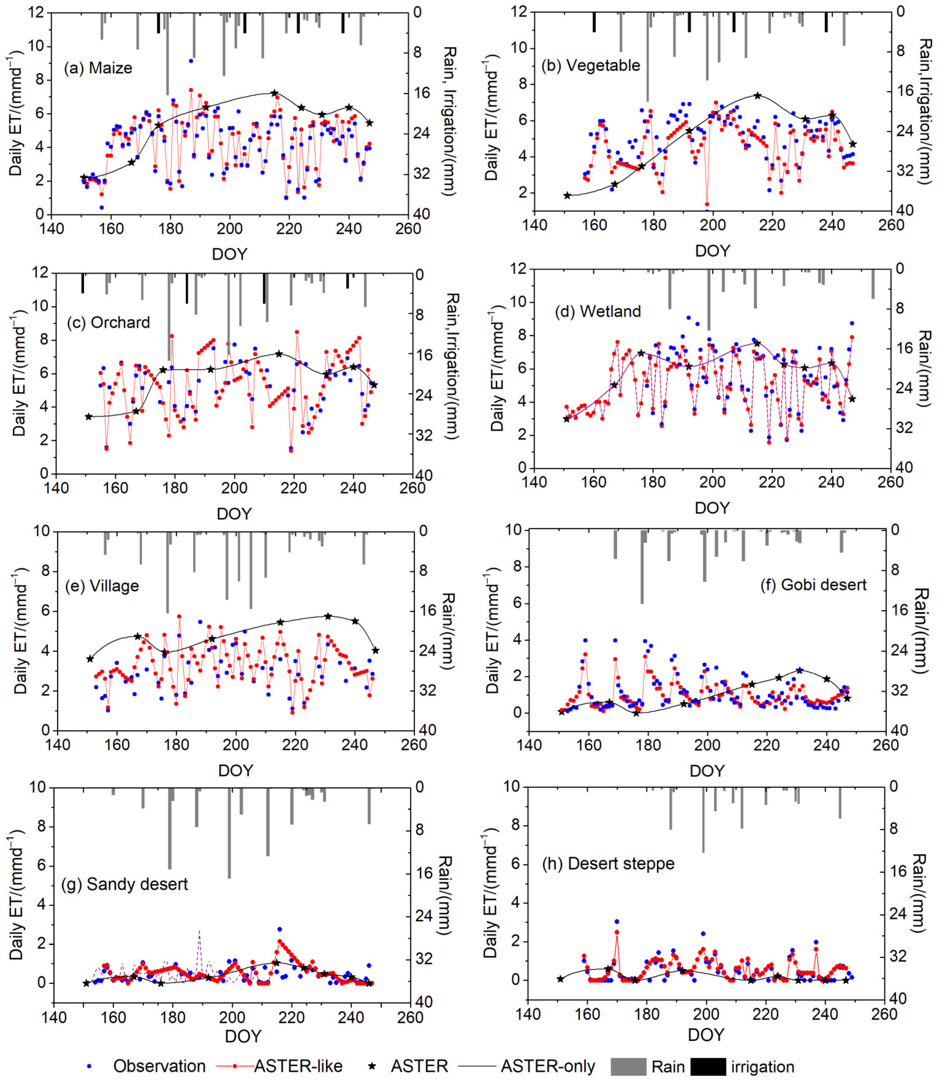
4.5. Temporal Patterns in Daily ET

Both the ASTER and synthetic ASTER-like daily ET streams were gap-filled to be continuous using a cubic spline interpolation. All ASTER-like results were compared with the observed ET in Figure 10. The results indicate that a good agreement was obtained between interpolated daily ET and observed daily ET, with RMSE, MAE, and MAP of 0.8 mm d⁻¹, 1.1 mm d⁻¹, and 13.4%, respectively. Figure 11 shows the temporal variation of ASTER-only and ASTER-like results at each of the eight flux tower sites. Clearly, ASTER, with a revisit period of 7–16 days, could hardly capture the temporal variation of daily ET values and was expected to result in large uncertainties. The role played by the MODIS ET in guiding the temporal interpolation of daily ET values between ASTER overpasses was evident from the fused time series. The complete time series of ASTER-like ET estimates generally produced reasonably accurate ET trends for all land-cover types. The day-to-day fluctuations in the ET data stream emphasized the detailed behavior of water stress, crop growth dynamics, and meteorological conditions at the different sites. For the sparsely vegetated sites (i.e., the Gobi Desert, sandy desert, and desert steppe), ET values were less than 1 mm d⁻¹, except for on rainy days. Additionally, the sporadic peaks of daily ET always occurred after rainfall events at these three sites, since the proportion of evaporation from bare soil was high. The fluctuations of daily ET values in vegetated areas covered by maize, vegetables, orchard, wetland, and village were clearly highly complex. Figure 6a–e highlights some significant differences among these sites for different vegetated surfaces, where the individual effects of soil evaporation, soil moisture storage, stomatal regulation, transpiration, and interception storage were all implicitly incorporated into the resulting surface evapotranspiration [52]. The u-STARFM is better able to capture the response of ET to rainfall and irrigation events. Spikes in ET usually occurred after rainfall or on days of irrigation. When precipitation occurred, the daily values of ET at all sites were relatively low, whereas they were relatively high after rainfall (DOY 174, 183, 193, 207). Additionally, peaks in ET values always occurred on days of irrigation (DOY 176, 205, 223, 238).

5. Conclusions

Measurements of continuous daily evapotranspiration (ET) at the field-scale are of substantial benefit for agricultural water management worldwide. The current lack of concurrent high spatial- and temporal-resolution remote sensing (RS) data significantly limits the applicability of RS-based methodologies. We proposed a data fusion framework for predicting continuous daily ET values at the field-scale by optimally exploiting the combined datasets of MODIS and ASTER. The STARFM algorithm, which was devised for producing Landsat surface reflectance time series, was modified and improved using a linear unmixing method (u-STARFM) for generating continuous daily ET estimates at the field-scale for heterogenous agricultural areas. In this study, an experiment was performed from July to September, 2012, in the middle reaches of the Heihe River Basin, Northwest China. Compared with the observed flux data, the synthetic fine-resolution daily ET estimates produced by the u-STARFM model had higher accuracies than those produced by STARFM, especially for heterogeneous agricultural areas.

Although the applications of data fusion to ET products from different satellite sensors is not straightforward, previous research has emphasized the potential advantages of STARFM for generating daily ET products with a high spatial and temporal resolution. However, STARFM often relies on the existence of “homogeneous” pixels at both fine- and coarse-resolution, which is more problematic for ET estimation than for reflectance or vegetation indices. The u-STARFM model presents several improvements over previous models. The most significant improvement is the ability to unmix coarse-resolution MODIS ET maps based on the abundance of land-cover types, and to replace the resampled MODIS ET values in the STARFM. The unmixed fraction of the unmixing data, which incorporates prior information about the MODIS ET values of each endmember in heterogeneous areas, can increase the probability of searching the “homogeneous” pixels and guarantee fusion accuracy. And the u-STARFM tends to outperform the original STARFM in irrigated heterogeneous agricultural areas, with overall MAP of 12.9% vs. 17.2%. Although many agricultural lands are smaller than one MODIS pixel, u-STARFM can adjust the daily ET changes of mixed MODIS pixels to the changes of internal ASTER pixels. Secondly, the land cover data was used as auxiliary information for the selection of similar pixels, which allowed more accurate similar pixels to be obtained. Thirdly, unlike ESTARFM, which requires at least two pairs of fine- and coarse-resolution images acquired on the same day, the u-STARFM needs just one input pair. Accordingly, in some cloudy regions, where it is difficult to acquire two high-quality input pairs simultaneously, u-STARFM may be more appropriate.

It should be noted that u-STARFM also contains a few limitations and constraints. Firstly, it assumes that the land-cover type is unchanged during the predicted period. Similar to STARFM and ESTARFM, u-STARFM cannot accurately predict transient changes that are not recorded in any of the base fine-resolution images. Therefore, combining u-STARFM with the STAARCH algorithm may be a feasible approach. Secondly, the size of the sliding window plays an important role in searching for similar pixels, and directly affects their weight distribution. The determination of sliding window size is not strictly regulated in the u-STARFM, being defined with an empirical or semi-quantitative method. Different study areas may require setting up different values, and it is necessary to perform a sensitivity analysis of different window sizes before the modeling.

In conclusion, u-STARFM improved the capability for producing daily ET products with both high-spatial resolution and frequent coverage from multi-source satellite data, which capture field-to-field variability in water usage. This information, if generated operationally, could be of utility for irrigation managers at the scale of individual fields, as well as for the regional monitoring of water use toward allocation and conservation efforts. Although the current study applied data fusion to ASTER and MODIS images, the techniques described here could be easily applied to other sensors. Further research could continue to analyze algorithm performance in various situations.

References

1. Katul, G.G.; Oren, R.; Manzoni, S.; Higgins, C.; Parlange, M.B. Evapotranspiration: A process driving mass transport and energy exchange in the soil-plant-atmosphere-climate system. Rev. Geophys. 2012, 50, RG3002. [Google Scholar] [CrossRef]
2. Anderson, M.C.; Allen, R.G.; Morse, A.; Kustas, W.P. Use of Landsat thermal imagery in monitoring evapotranspiration and managing water resources. Remote Sens. Environ. 2012, 122, 50–65. [Google Scholar] [CrossRef]
3. Magali, O.L.; Isidro, C.; Christopher, M.U.N.; Samuel, O.F.; Carlos, P.E.; Claudio, B.; Alfonso, C. Estimating Evapotranspiration of an Apple Orchard Using a Remote Sensing-Based Soil Water Balance. Remote Sens. 2016, 8, 253. [Google Scholar] [CrossRef]
4. Wu, X.J.; Zhou, J.; Wang, H.J.; Li, Y.; Zhong, B. Evaluation of irrigation water use efficiency using remote sensing in the middle reach of the Heihe river, in the semi-arid Northwestern China. Hydrol. Process. 2015, 29, 2243–2257. [Google Scholar] [CrossRef]
5. Yang, Y.T.; Shang, S.H.; Jiang, L. Remote sensing temporal and spatial patterns of evapotranspiration and the responses to water management in a large irrigation district of North China. Agric. For. Meteorol. 2012, 164, 112–122. [Google Scholar] [CrossRef]
6. Hu, G.C.; Jia, L. Monitoring of Evapotranspiration in a Semi-Arid Inland River Basin by Combining Microwave and Optical Remote Sensing Observations. Remote Sens. 2015, 7, 3056–3087. [Google Scholar] [CrossRef] [Green Version]
7. Nagler, P.L.; Morino, K.; Murray, R.S.; Osterberg, J.; Glenn, E.P. An empirical algorithm for estimating agricultural and riparian evapotranspiration using MODIS enhanced vegetation index and ground measurements of ET. I. Description of method. Remote Sens. 2009, 1, 1273–1297. [Google Scholar] [CrossRef]
8. Bastiaanssen, W.G.M.; Menenti, M.; Feddes, R.A.; Holtslag, A.A.M. A remote sensing surface energy balance algorithm for land (SEBAL)1. Formulation. J. Hydrol. 1998, 212–213, 198–212. [Google Scholar] [CrossRef]
9. Su, Z. The Surface Energy Balance System (SEBS) for estimation of turbulent heat fluxes. Hydrol. Earth Syst. Sci. 2002, 6, 85–99. [Google Scholar] [CrossRef]
10. Allen, R.G.; Tasumi, M.; Trezza, R. Satellite-based energy balance for mapping evapotranspiration with internalized calibration (METRIC)-model. J. Irrig. Drain. Eng. 2007, 133, 380–394. [Google Scholar] [CrossRef]
11. Kustas, W.P.; Norman, J.M. A two-source approach for estimating turbulent fluxes using multiple angle thermal infrared observations. Water Resour. Res. 1997, 33, 1495–1508. [Google Scholar] [CrossRef] [Green Version]
12. Leuning, R.; Zhang, Y.Q.; Rajaud, A.; Cleugh, H.; Tu, K. A simple surface conductance model to estimate regional evaporation using MODIS leaf area index and the Penman-Monteith equation. Water Resour. Res. 2008, 44, 652–655. [Google Scholar] [CrossRef]
13. Yao, Y.J.; Liang, S.L.; Li, X.L.; Chen, J.Q.; Wang, K.C.; Jia, K. A satellite-based hybrid algorithm to determine the Priestley-Taylor parameter for global terrestrial latent heat flux estimation across multiple biomes. Remote Sens. Environ. 2015, 165, 216–233. [Google Scholar] [CrossRef]
14. Huang, C.L.; Chen, W.J.; Li, Y.; Shen, H.F.; Li, X. Assimilating multi-source data into land surface model to simultaneously improve estimations of soil moisture, soil temperature, and surface turbulent fluxes in irrigated fields. Agric. Forest Meteorol. 2016, 230–231, 142–156. [Google Scholar] [CrossRef]
15. Hartanto, I.M.; van der Kwast, J.; Alexandridis, T.K.; Almeida, W.; Song, Y.; van Andel, S.J.; Solomatine, D.P. Data assimilation of satellite-based actual evapotranspiration in a distributed hydrological model of a controlled water system. Int. J. Appl. Earth Observ. Geoinf. 2017, 57, 123–135. [Google Scholar] [CrossRef]
16. Yang, Y.T. Evapotranspiration over Heterogeneous Vegetated Surfaces. Ph.D. Thesis, Tsinghua University, Beijing, China, 2015. [Google Scholar]
17. Wang, K.; Dickinson, R.E. A review of global terrestrial evapotranspiration: Observation, modelling, climatology, and climatic variability. Rev. Geophys. 2011, 50, 1–54. [Google Scholar] [CrossRef]
18. Verstraeten, W.W.; Veroustraete, F.; Feyen, J. Assessment of Evapotranspiration and Soil Moisture Content across Different Scales of Observation. Sensors 2008, 8, 70–117. [Google Scholar] [CrossRef] [PubMed]
19. Evett, S.R.; Kustas, W.P.; Gowda, P.H.; Anderson, M.C.; Prueger, J.H.; Howell, T.A. Overview of the Bushland Evapotranspiration and Agricultural Remote sensing EXperiment 2008 (BEAREX08): A field experiment evaluating methods for quantifying ET at multiple scales. Adv. Water Resour. 2012, 50, 4–19. [Google Scholar] [CrossRef]
20. Kustas, W.P.; Li, F.; Jackson, T.J.; Prueger, J.H.; MacPherson, J.I.; Wolde, M. Effects of remote sensing pixel resolution on modeled energy flux variability of croplands in Iowa. Remote Sens. Environ. 2004, 92, 535–547. [Google Scholar] [CrossRef]
21. He, R.Y.; Jin, Y.F.; Kandelous, M.M.; Zaccaria, D.; Sanden, B.L.; Snyder, R.L.; Jiang, J.B.; Hopmans, J.W. Evapotranspiration Estimate over an Almond Orchard Using Landsat Satellite Observations. Remote Sens. 2017, 9, 436. [Google Scholar] [CrossRef]
22. Senay, G.B.; Friedrichs, M.; Singh, R.K.; Velpuri, N.M. Evaluating Landsat 8 evapotranspiration for water use mapping in the Colorado River Basin. Remote Sens. Environ. 2016, 185, 171–185. [Google Scholar] [CrossRef]
23. McCabe, M.F.; Wood, E.F. Scale Influences on the Remote Estimation of Evapotranspiration Using Multiple Satellite Sensors. Remote Sens. Environ. 2006, 105, 271–285. [Google Scholar] [CrossRef]
24. Singh, R.K.; Senay, G.B.; Velpuri, N.M.; Bohms, S.; Verdin, J.P. On the Downscaling of Actual Evapotranspiration Maps Based on Combination of MODIS and Landsat-Based Actual Evapotranspiration Estimates. Remote Sens. 2014, 6, 10483–10509. [Google Scholar] [CrossRef] [Green Version]
25. Ke, Y.H.; Im, J.H.; Park, S.; Gong, H.L. Downscaling of MODIS One Kilometer Evapotranspiration Using Landsat-8 Data and Machine Learning Approaches. Remote Sens. 2016, 8, 215. [Google Scholar] [CrossRef]
26. Gao, F.; Masek, J.; Schwaller, M.; Hall, F. On the Blending of the Landsat and MODIS Surface Reflectance: Predicting Daily Landsat Surface Reflectance. IEEE Trans. Geosci. Remote Sens. 2006, 44, 2207–2218. [Google Scholar]
27. Bhandari, S.; Phinn, S.; Gill, T. Preparing Landsat Image Time Series (LITS) for Monitoring Changes in Vegetation Phenology in Queensland, Australia. Remote Sens. 2012, 4, 1856–1886. [Google Scholar] [CrossRef] [Green Version]
28. Li, X.D.; Ling, F.; Foody, M.G.; Ge, Y.; Zhang, Y.H.; Du, Y. Generating a series of fine spatial and temporal resolution land cover maps by fusing coarse spatial resolution remotely sensed images and fine spatial resolution land cover maps. Remote Sens. Environ. 2017, 196, 293–311. [Google Scholar] [CrossRef] [Green Version]
29. Weng, Q.H.; Fu, P.; Gao, F. Generating Daily Land Surface Temperature at Landsat Resolution by Fusing Landsat and MODIS data. Remote Sens. Environ. 2014, 45, 55–67. [Google Scholar] [CrossRef]
30. Yang, G.J.; Weng, Q.H.; Pu, R.L.; Gao, F.; Sun, C.H.; Li, H.; Zhao, C.J. Evaluation of ASTER-Like Daily Land Surface Temperature by Fusing ASTER and MODIS Data during the HiWATER-MUSOEXE. Remote Sens. 2016, 8, 75. [Google Scholar] [CrossRef]
31. Cammalleri, C.; Anderson, M.C.; Gao, F.; Hain, C.R.; Kustas, W.P. A Data Fusion Approach for Mapping Daily Evapotranspiration at Field Scale. Water Resour. Res. 2013, 49, 4672–4686. [Google Scholar] [CrossRef]
32. Cammalleri, C.; Anderson, M.C.; Gao, F.; Hain, C.R.; Kustas, W.P. Mapping Daily Evapotranspiration at Field Scales over Rainfed and Irrigated Agricultural Areas Using Remote Sensing Data Fusion. Agric. For. Meteorol. 2014, 186, 1–11. [Google Scholar] [CrossRef]
33. Yang, Y.; Anderson, M.C.; Gao, F.; Hain, C.R.; Semmens, K.A.; Kustas, W.P.; Noormets, A.; Wynne, R.H.; Thomas, V.A.; Sun, G. Daily Landsat-scale Evapotranspiration Estimation over a Forested Landscape in North Carolina, USA Using Multi-satellite Data Fusion. Hydrol. Earth Syst. Sci. 2016, 21, 1017–1037. [Google Scholar] [CrossRef]
34. Semmens, K.A.; Anderson, M.C.; Kustas, W.P.; Gao, F.; Alfieri, J.G.; McKee, L.; Prueger, J.H. Monitoring Daily Evapotranspiration over Two California Vineyards Using Landsat 8 in a Multi-sensor Data Fusion Approach. Remote Sens. Environ. 2016, 185, 155–170. [Google Scholar] [CrossRef]
35. Li, Y.; Huang, C.L.; Hou, J.L.; Gu, J.; Zhu, G.F.; Li, X. Mapping Daily Evapotranspiration Based on Spatiotemporal Fusion of ASTER and MODIS Images over Irrigated Agricultural Areas in the Heihe River Basin, Northwest China. Agric. For. Meteorol. 2017, 244–245, 82–97. [Google Scholar] [CrossRef]
36. Hilker, T.; Wulder, M.A.; Coops, N.C.; Linke, J.; McDermid, G.; Masek, J.G.; Gao, F.; White, J.C. A new data fusion model for high spatial- and temporal-resolution mapping of forest disturbance based on Landsat and MODIS. Remote Sens. Environ. 2009, 113, 1613–1627. [Google Scholar] [CrossRef]
37. Zhu, X.L.; Chen, J.; Gao, F.; Chen, X.H.; Masek, J.G. An Enhanced Spatial and Temporal Adaptive Reflectance Fusion Model for Complex Heterogeneous Regions. Remote Sens. Environ. 2010, 114, 2610–2623. [Google Scholar] [CrossRef]
38. Fu, D.J.; Chen, B.Z.; Wang, J.; Zhu, X.L.; Hilker, T. An Improved Image Fusion Approach Based on Enhanced Spatial and Temporal the Adaptive Reflectance Fusion Model. Remote Sens. 2013, 5, 6346–6360. [Google Scholar] [CrossRef] [Green Version]
39. Bai, L.L.; Cai, J.B.; Liu, Y.; Chen, H.; Zhang, B.Z.; Huang, L.X. Responses of field evapotranspiration to the changes of cropping pattern and groundwater depth in large irrigation district of Yellow River basin. Agric. Water Manag. 2017, 188, 1–11. [Google Scholar] [CrossRef]
40. Yi, Z.Y.; Zhao, H.L.; Jiang, Y.Z.; Yan, H.W.; Cao, Y.; Huang, Y.Y.; Hao, Z. Daily Evapotranspiration Estimation at the Field Scale: Using the Modified SEBS Model and HJ-1 Data in a Desert-Oasis Area, Northwestern China. Water 2018, 10, 640. [Google Scholar] [CrossRef]
41. Zhang, M.M.; Wang, S.; Fu, B.J.; Gao, G.Y.; Shen, Q. Ecological effects and potential risks of the water diversion project in the Heihe River Basin. Sci. Total Environ. 2018, 619–620, 794–803. [Google Scholar] [CrossRef] [PubMed]
42. Li, X.; Liu, S.M.; Xiao, Q.; Ma, M.G.; Jin, R.; Che, T.; Wang, W.Z.; Hu, X.L.; Xu, Z.W.; Wen, J.G.; et al. A multiscale dataset for understanding complex eco-hydrological processes in a heterogeneous oasis system. Sci. Data 2017, 4, 170083. [Google Scholar] [CrossRef] [PubMed] [Green Version]
43. Xu, Z.W.; Liu, S.M.; Li, X.; Shi, S.J.; Wang, J.M.; Zhu, Z.L.; Xu, T.R.; Wang, W.; Ma, M. Intercomparison of surface energy flux measurement systems used during the HiWATER-MUSOEXE. J. Geophys. Res. Atmos. 2013, 118, 13140–13157. [Google Scholar] [CrossRef]
44. Estévez, J.; Gavilán, P.; Giráldez, J.V. Guidelines on validation procedures for meteorological data from automatic weather stations. J. Hydrol. 2011, 402, 144–154. [Google Scholar] [CrossRef] [Green Version]
45. Estévez, J.; García-Marín, A.P.; Morábito, J.A.; Cavagnaro, M. Quality assurance procedures for validating meteorological input variables of reference evapotranspiration in mendoza province (Argentina). Agric. Water Manag. 2016, 172, 96–109. [Google Scholar] [CrossRef]
46. Xu, Z.W.; Ma, Y.F.; Liu, S.M.; Shi, W.J.; Wang, J.M. Assessment of the Energy balance closure under advective conditions and its impact using remote sensing data. J. Appl. Meteorol. Climatol. 2017, 56, 127–140. [Google Scholar] [CrossRef]
47. Li, H.; Sun, D.L.; Yu, Y.Y.; Wang, H.Y.; Liu, Y.L.; Liu, Q.H.; Du, Y.M.; Wang, H.; Cao, B. Evaluation of the VIIRS and MODIS LST Products in an Arid Area of Northwest China. Remote Sens. Environ. 2014, 142, 111–121. [Google Scholar] [CrossRef]
48. Zhong, B.; Yang, A.X.; Nie, A.H.; Yao, Y.J.; Zhang, H.; Wu, S.L.; Liu, Q.H. Finer Resolution Land-Cover Mapping Using Multiple Classifiers and Multisource Remotely Sensed Data in the Heihe River Basin. IEEE J. Sel. Top. Appl. Earth Obs. Remote Sens. 2015, 99, 1–20. [Google Scholar] [CrossRef]
49. Zhao, J.; Li, J.; Liu, Q.H.; Fan, W.J.; Zhong, B.F.; Wu, S.L.; Yang, L.; Zeng, Y.L.; Xu, B.D.; Yin, G.F. Leaf Area Index Retrieval Combining HJ1/CCD and Landsat8/OLI Data in the Heihe River Basin, China. Remote Sens. 2015, 7, 6862–6885. [Google Scholar] [CrossRef] [Green Version]
50. Kustas, W.P.; Daughtry, C.S.T. Estimation of the soil heat flux/net radiation ratio from spectral data. Agric. For. Meteorol. 1990, 49, 205–223. [Google Scholar] [CrossRef]
51. Gokmen, M.; Vekerdy, Z.; Verhoef, A.; Verhoef, W.; Batelaan, O.; van der Tol, C. Integration of soil moisture in SEBS for improving evapotranspiration estimation under water stress conditions. Remote Sens. Environ. 2012, 121, 261–274. [Google Scholar] [CrossRef]
52. Huang, C.L.; Li, Y.; Gu, J.; Lu, L.; Li, X. Improving Estimation of Evapotranspiration under Water-Limited Conditions Based on SEBS and MODIS Data in Arid Regions. Remote Sens. 2015, 7, 16795–16814. [Google Scholar] [CrossRef] [Green Version]
53. Li, Y.; Zhou, J.; Wang, H.J.; Li, D.Z.; Jin, R.; Zhou, Y.Z.; Zhou, Q.G. Integrating soil moisture retrieved from L-band microwave radiation into an energy balance model to improve evapotranspiration estimation on the irrigated oases of arid regions in northwest China. Agric. Forest Meteorol. 2015, 214–215, 306–318. [Google Scholar] [CrossRef]
54. Ghulam, A.; Qin, Q.M.; Teyip, T.; Li, Z.L. Modified perpendicular drought index (MPDI): A real-time drought monitoring method. ISPRS J. Photogramm. Remote Sens. 2007, 62, 150–164. [Google Scholar] [CrossRef]
55. Settle, J.J.; Drake, N. Linear Mixing and the Estimation of Ground Cover Proportions. Int. J. Remote Sens. 1993, 14, 1159–1177. [Google Scholar] [CrossRef]
56. Zhang, Y.; Li, L.; Chen, L.Q.; Liao, Z.H.; Wang, Y.C.; Wang, B.Y.; Yang, X.Y. A Modified Multi-Source Parallel Model for Estimating Urban Surface Evapotranspiration Based on ASTER Thermal Infrared Data. Remote Sens. 2017, 9, 1029. [Google Scholar] [CrossRef]
57. Xie, D.F.; Zhang, J.S.; Zhu, X.F.; Pan, Y.Z.; Liu, H.L.; Yuan, Z.M.Q.; Yun, Y. An Improved STARFM with Help of an Unmixing-Based Method to Generate High Spatial and Temporal Resolution Remote Sensing Data in Complex Heterogeneous Regions. Sensors 2016, 16, 207. [Google Scholar] [CrossRef] [PubMed]
Figure 1. The experimental region and field observation system.
Remotesensing 10 01694 g001
Figure 2. Schematic overview of the inputs and processing steps in the evapotranspiration (ET) data fusion system. (NDVI: normalized difference vegetation index; LST: land surface temperature; MPDI: the modified perpendicular drought index; MODIS: the moderate resolution imaging spectroradiometer; ASTER: the advanced space-borne thermal emission reflectance radiometer; STARFM: spatial and temporal adaptive reflectance fusion model; u-STARFM: the modified STARFM model)
Remotesensing 10 01694 g002
Figure 3. Schematic description of the data fusion procedure.
Remotesensing 10 01694 g003
Figure 4. A comparison of the modeled and observed surface heat fluxes at the eight experimental sites from 30 May to 12 September, 2012. (a) Shows scatter plots of the modeled and observed sensible heat fluxes (H); and (b) shows scatter plots of the modeled and observed latent heat fluxes (λET). Red and black symbols represent ASTER and MODIS data, respectively.
Remotesensing 10 01694 g004
Figure 5. Scatter plots of observed and simulated daily ET, by u-STARFM (blue dots) and STARFM (black dots), for the Gobi Desert (a); desert steppe (b); sandy desert (c); wetland (d); village (e); vegetable (f); orchard (g); and maize (h).
Remotesensing 10 01694 g005
Figure 6. Spatial pattern, magnified view, and frequency distribution of ET maps, on 15 June, from: (a) MODIS; (b) unmixing method; (c) ASTER; (d) fusion using STARFM; and (e) u-STARFM model. Field boundaries were overlaid to compare inter- and intra-field variability in ET.
Remotesensing 10 01694 g006
Figure 7. Histograms for: (a) MODIS ET and ASTER ET; (b) unmixing ET; (c) ASTER-like ET based on the STARFM model and ASTER ET; and (d) ASTER-like ET based on the u-STARFM model and ASTER ET, on 15 June.
Remotesensing 10 01694 g007
Figure 8. Spatial pattern, magnified view and frequency distribution of ET maps, on 2 August, from: (a) MODIS; (b) unmixing; (c) ASTER; (d) fusion using the STARFM model; and (e) fusion using the u-STARFM model. Field boundaries were overlaid to compare inter- and intra-field variability in ET.
Remotesensing 10 01694 g008
Figure 9. Histograms for: (a) MODIS ET and ASTER ET; (b) unmixing ET; (c) ASTER-like ET based on the STARFM model and ASTER ET; and (d) ASTER-like ET based on the u-STARFM model and ASTER ET, on 2 August.
Remotesensing 10 01694 g009
Figure 10. A comparison of the continuous daily ET by interpolation and observed daily ET.
Remotesensing 10 01694 g010
Figure 11. Time series of observed ET (blue dots), daily ET estimates from u-STARFM (red line with dots), and ASTER ET (black pentagram and line) from May to September, 2012. Rainfall and irrigation events are shown as blue and grey bars, respectively.
Remotesensing 10 01694 g011