Improving Land Cover Classifications with Multiangular Data: MISR Data in Mainland Spain


1
Departamento de Tecnología Química y Ambiental, ESCET, Universidad Rey Juan Carlos, C/Tulipán s/n, 28933 Móstoles, Spain
2
Geography Group, Departamento de Ciencias de la Educación, Lenguaje, Cultura y Artes, Ciencias Histórica-Jurídicas y Humanísticas y Lenguas Modernas, Facultad de Ciencias Jurídicas y Sociales, Universidad Rey Juan Carlos, Paseo de los Artilleros s/n, 28032 Madrid, Spain
*
Authors to whom correspondence should be addressed.
Remote Sens. 2018, 10(11), 1717; https://0-doi-org.brum.beds.ac.uk/10.3390/rs10111717
Submission received: 23 August 2018
/
Revised: 18 October 2018
/
Accepted: 24 October 2018
/
Published: 31 October 2018
(This article belongs to the Special Issue MISR)
Abstract
:In this study, we deal with the application of multiangular data from the Multiangle Imaging Spectroradiometer (MISR) sensor for studying the effect of surface anisotropy and directional information on the classification accuracy for different land covers with different rate of disaggregation classes (from four to 35 different classes) from a Mediterranean bioregion in Iberian, Spain. We used various MISR band groups from nadir to blue, green, red, and NIR channels at nadir and off-nadir. The MISR data utilized here were provided by the L1B2T product (275 m spatial resolution) and belonged to two different orbits. We performed 23 classifications with the k-means algorithm to test multiangular data, number of clusters, and iteration effects. Our findings confirmed that the multiangular information, in addition to the multispectral information used as the input of the k-means algorithm, improves the land cover classification accuracy, and this improvement increased with the level of disaggregation. A very large number of clusters produced even better improvements than multiangular data.
1. Introduction
Remote sensing techniques offer a unique environmental monitoring capability that covers large geographical areas in a cost-efficient manner. This science can capture important information about the Earth´s land, atmosphere, and body of waters. Remote sensing products have been usefully employed in numerous applications, for instance, carbon emission monitoring [1,2,3], land change detection [4], forest monitoring [5,6], natural hazard assessment [7,8], agriculture and water/wetland monitoring [9,10,11,12], climate dynamics [13,14,15,16], and biodiversity studies [17,18,19]. One of the applications of remote sensing is to classify images to obtain classified maps. Classification in remote sensing groups the pixels of an image into a set of classes, such that pixels in the same category have similar properties. Most of the image classifications are based on the detection of the spectral response patterns of land cover classes [20]. Traditional remote sensing classification depends on distinctive signatures for the land cover categories or types in the band set that is being used. It regards the ability to distinguish these signatures from other spectral response patterns that may be present [21]. The application of remote sensing data for land cover and land use mapping, and their changes, is key to many diverse applications that have been mentioned before [22,23].
Land Use and Land Cover (LULC) mapping using satellite or airborne imagery has increased exponentially over the past decades. This growth is due in part to the wide availability of sensors, such as the Moderate Resolution Imaging Spectroradiometer (MODIS), MEdium Resolution Imaging Spectrometer (MERIS), Landsat, Sentinel, Satellite for observation of Earth (SPOT), aerial photography, and drones, that generate satellite imagery of an adequate spatial resolution at different temporal or angular resolutions. It is also due to improved data availability and accessibility of the sources of remote sensing information [22].
Many approaches exist to classify remote sensing data. However, these converge into three principal methods: supervised, unsupervised, and hybrid classification techniques. Supervised classification requires prior knowledge of the ground cover in the study area. There are some examples in which multispectral or hyperspectral data are used as the input of pixel information to train a classification algorithm [24]. Some supervised methods are the maximum likelihood, Spectral Angle Mapper [25], Support Vector Machine [26,27], and Decision Trees [28]. These methods group pixels around training samples and a classified image has the same training classes. However, in unsupervised classification, an algorithm finds a prespecified amount of statistical clusters in multispectral or hyperspectral space. Usually, these groups are not equivalent to actual classes of land cover; however, this method can be used without having prior knowledge of the ground cover in the study site [29]. Some unsupervised techniques are k-means, principal components, and autoencoder [30]. Hybrid methods, meanwhile, involve firstly applying an unsupervised classification and then a supervised one [31]. An important issue when a classification experiment is developing is the accuracy of the final product. In this sense, some authors affirm that the accuracy of the results obtained by using unsupervised classification is similar to those of the supervised approach [31,32].
Although the most common basis of classification is multispectral and hyperspectral information, sometimes and in some zones to classify or map LULC, there are classes that overlap regarding the mean, median, or standard deviation in a single spectral band at a single date. Thereby, the final accuracy of classification will also decrease due to the overlapping. This problem may be solved by using, in addition to the multispectral or hyperspectral data as the input algorithm, multiangular information. Ever since the first data obtained by satellite in the 1970s, it has been possible to observe the fact that the reflectance of different land covers is dependent on the observation and illumination angles. That dependence implied that the land covers are anisotropic, that is, they did not reflect the same amount of energy in all directions. The magnitude best explained that reflectance is dependent on both the observation and illumination angles and the wavelength of the reflected radiation [33] is the Bidirectional Reflectance Function (BRDF) that, if referred to a Lambertian object, is called the Bidirectional Reflectance Factor (BRF).
The anisotropy that different terrestrial surfaces present was considered as an avenue to explore. For its study, the launch of satellites with sensors onboard was promoted. These sensors have allowed the study of the different directional behaviors when a target reflects solar radiation [34]; prominent examples include the POLarization and Directionality of the Earth’s Reflectances (POL-DER) instrument, the multiangle Imaging Spectro-Radiometer (MISR), and the Compact High-Resolution Imaging Spectrometer (CHRIS Proba). The last two can capture images of almost the same pixel from several different angles during the same flight path [35]. In this manner, it is easy to find studies where MISR products have been successfully used. Various authors (e.g., [36,37,38,39,40]) have proven their utility for characterizing the vegetal canopy and for mapping vegetation and land covers at medium and large spatial scales.
This paper deals with the application of multiangular MISR data to study the effect of surface anisotropy and directional information on the classification accuracy of almost pure pixels of different land covers with a different rate of disaggregation classes in mainland Spain. Some authors have improved the classification accuracy by using multiangular and multispectral remote sensing information [41,42,43,44,45,46]. For instance, Abuelgasim et al. [41] classified five different land covers using the Advanced Solid-State Array Spectroradiometer (ASAS) in Voyageurs National Park, Minnesota. These authors used an artificial neural network method and achieved an improvement of 1% in accuracy by using the multiangular and multispectral information (89%) over using only that which is multispectral (88%). Additionally, Hyman and Barnsley [42] attempted to classify three different Amazonian forest land cover types with MISR data, applying both Principal Components Analysis (PCA) and the minimum distance algorithm as classification techniques. These authors demonstrated that data acquisition in off-nadir viewing improved the discrimination and mapping of the land cover types overall using the −21.6° view angle, for which accuracies improved by 16.3% (from 78.5% to 95.0%) compared with those for the nadir view. Furthermore, Liesenberg et al. [44] performed classification with MISR data to map three types of forest (from close to open vegetation forest) in the Brazilian savanna. These last authors used the maximum likelihood classification technique, and found that multiangular information could help to distinguish between those classes that are homogenous for the multispectral indicators. Mahtab et al. [45] used MISR data from different dates in two different years. Their study area was Madhya Pradesh, India, and they performed PCA and used a parallelepiped classifier. The authors also found that multiangular information, in combination with multispectral (green, red, and NIR) data, resulted in high classification accuracies for all the dates that they used. Likewise, Su et al. [46] were able to classify arid and semiarid dessert grassland classes located in the Chihuahuan semi-desert province, in New Mexico, by using MISR and MODIS multiangular and multispectral data. Using maximum likelihood and the Support Vector Machine (SVM), the authors achieved results that rounded from 45.8% using nadir reflectance as the input of classification, to 76.7% using SVM algorithms and multiangular and multispectral information combined as the input of classification. Many others studies have also shown that MISR multiangular data can be used to obtain vegetation structure information, such as canopy cover and canopy height [39,47,48,49,50,51,52,53,54]. Therefore, MISR multiangular data show great potential to obtain improved low-to-medium resolution regional land cover maps [26,44,45,46,55], differentiating classes from the structural point of view.
Against this background, our objective was to assess the possible beneficial effect of incorporating multiangle information in the classification of images in many types of land cover in mainland Spain. An improvement in classification accuracy was expected, but we wanted to know how this improvement was dependent on the level of disaggregation and how land covers were disaggregated. We additionally wanted to test the effects of changing parameters of unsupervised methods, and their relationship with different levels of class aggregation.
2. Materials and Methods
2.1. Study Site
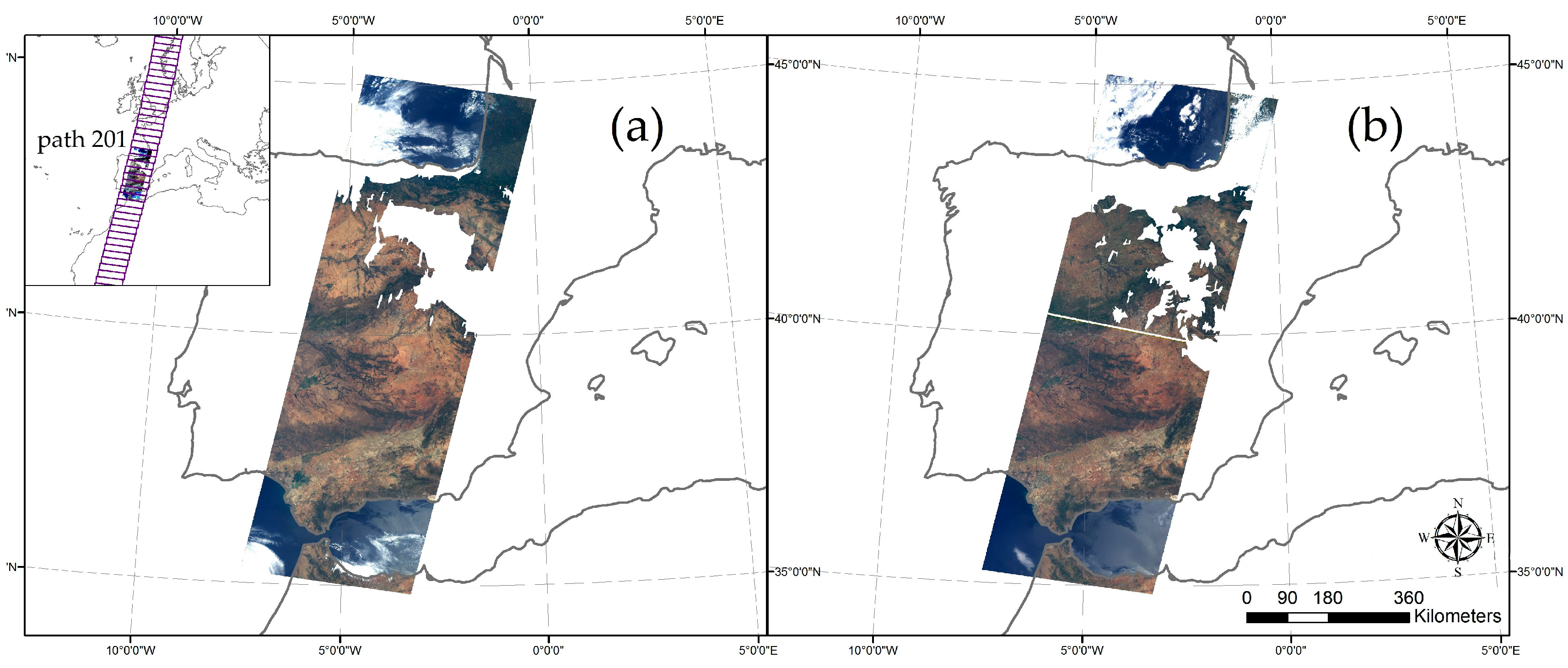
The study area in this research was the intersection of MISR path 201, and mainland Spain. This area starts in MISR Block 56 and ends in Block 61 (See Figure 1). Mainland Spain has a wide variety of natural surfaces and is an example of the Mediterranean zone.
2.2. MISR and MISR Data
MISR is a sensor boarded on the Earth Observing System (EOS) Terra satellite with a 705 km sun-synchronous Earth orbit. The MISR instrument has nine push cameras capable of viewing the Earth’s surface from different angles (nominal and design values), namely 0° (An), 26.1° (Af, Aa), 45.6° (Bf, Ba), 60.0° (Cf, Ca), and 70.5° (Df, Da), relative to nadir. In both, (f) corresponds to forward and (a) is relative to afterward, along the direction of the flight. This sensor obtains Earth information in four spectral bands positioned at 446, 558, 672, and 866 nm, with a temporal resolution of two to nine days and a spatial resolution of either 1100 or 275 m [56].
The MISR team provides several elaborated data products with different processing levels. In this study, we used MI1B2T to classify and MIL2ASLS to atmospherically correct one of the MI1B2 images. The first two products are available at a 275 m spatial resolution, and the last one at a 1100 m spatial resolution. The MI1B2T gives radiance values and a scalar element to convert them into the BRF. The MIL2ASLS provides the BRF, The Rahman–Pinty–Verstraete Modified (MRPV) parameters of BRF, the Aerosol Optical Depth (AOD), and some quality-related values [56].
We classified two MISR MI1B2T images. The first one was from orbit 29476 and was obtained on 3 July 2005, and the second was from orbit 45320 and was obtained on 25 July 2008. Both are from MISR product version F03-0024. Image 29476 was atmospherically corrected to study possible improvement. The data belonged to MISR path 201. The image from 2006 was selected because the land cover map used to evaluate improvement was from 2006, while the image from 2008 was chosen to maximize common zones but with the same month.
2.3. CORINE Land Cover 2006
The CORINE (Co-ordination of Information on the Environment) land cover (CLC) consists of a set of maps of the European environmental landscape, based on the photographic interpretation of satellite images (SPOT, LANDSAT TM, and MSS). Ancillary data (aerial photographs, topographic and vegetation maps, statistics, and local knowledge) were used to improve the interpretation and the assignments of the territory into the categories of the CLC nomenclature. The smallest surfaces mapped corresponded to 25 hectares, and the minimum mapping width was 100 m [57]. General accuracy was 87.1% in CORINE 2000 version [58], and individual class reliability ranged from 12.5% to 100%. The CORINE 2006 version was evaluated by testing changes between 2000 and 2006, and the accuracy of these changes was found to be 87.82% [59]. This project presents comparable digital maps of land cover (and partly land use) for each country based on the terminology of 44 categories organized hierarchically in three levels.
In this work, we used the map from Spain, which consisted of a 1:100,000 vectorial layer from 2006.
To evaluate the reliability of the MISR classification results, we used the occupancy map of the CORINE Land Cover 2006 three levels of depth, taking as a reference almost 200,000 points included in a buffer of 137.5 m of ratio, to ensure that we obtained pixels with the presence of only one of the CORINE classes.
There were 35 initial reference classes for the maximum disaggregation; we did not consider all of the 44 classes because nine classes had no points. We grouped these categories in different ways to evaluate up to seven levels of differentiation. We started the experiment with the five classes of CORINE level 1. The classification groups are listed in Table 1.
2.4. Data Processing and Data Analysis
The MI1B2T, MIL2ASLS, and MIB2GEOP data from the two MISR schemes at the blue, green, red, and NIR band were downloaded from the NASA Langley Distributed Active Archive Center (DAAC). Then, the data from the Space Oblique Mercator (SOM) were re-projected to the Universal Transverse Mercator (UTM) system, the MI1B2T radiances were transformed into BRF values using the scalar factor also provided on that product, and a visual cloud mask was applied to avoid cloud contamination.
Orbit 29476 was subjected to an atmospheric correction based on regression with data from the MIL2ASLS 1.1 km × 1.1 km product. This method has been used by other authors [60,61]. The process consists of taking advantage of the atmospheric correction routine performed by the MISR Team to obtain the MIL2ASLS product with data obtained thanks to the AOD estimation. AOD is estimated at a coarser 17.6 km × 17.6 km spacing, so every square is atmospherically corrected independently. This method occasionally produces a quilting effect. Through a regression per every square of 17.6 km between the product MI1B2T aggregated to 1.1 km, and the MIL2ASLS, we performed an atmospheric correction of the BRF values of the MISR bands belonging to the first product (MI1B2T). Those pixels in which the correlation coefficient per square between the two products was less than 0.9 were excluded. Figure 2 displays the masking effect of this method due to the absence of data squares in the MIL2ASLS product.
As we were interested in evaluating multiangular data improvement in classification, we decided to use an unsupervised classification method to allow self-clustering of that data. Additionally, unsupervised methods are more flexible for assessing different parametrizations of the experiments. The k-means algorithm was used to classify the MISR images. The k-means algorithm belongs to the group of unsupervised classifiers since it does not use a previous sample of points by classes to classify; rather, it seeks to group the data in terms of the number of types that are indicated, minimizing intra-group variability, by reducing the distances between each point and the average of its class [20].
The allocation of data was done iteratively. Thus, the calculation and reassignment were performed in classes in each step. For this reason, the initial points that are taken as class representatives may have great importance in the final classification, since the initial classes are built around them [20]. To avoid such interference, and to evaluate this parameter’s importance, the process was performed with a large number of categories, allowing a good representation of searched typologies and a high number of iterations, enabling large data transfers between classes. The primary factors that were modified were the number of categories, the bands to be taken into account, and the number of iterations. Two different images were used, one of which was corrected atmospherically to check if such correction had any effect on the result.
The different band groups used to classify were: (i) the four zenithal, (G-An, B-An, R-An, and NIR-An), i.e., the typical multispectral information; (ii) the zenithal plus the four nearer nadir (G-An, B-An, R-An, NIR-An, R-Bf, R-Af, R-Ba, and R-Bf); (iii) only multiangle information, the nine bands of red (R-An, R-Bf, R-Af, R-Ba, R-Bf, R-Cf, R-Cf, R-Da, and R-Df); and (iv) all available (G-An, B-An, R-An, NIR-An, R-Bf, R-Af, R-Ba, R-Bf, R-Cf, R-Cf, R-Da, and R-Df). We chose to test the effect of taking into account only multispectral information, only multiangle information, and combinations of both with all existing bands, and without taking into account the most external cameras (which are those that have topographical hiding problems but have essential multiangular information). We excluded points without all nine bands of data to avoid missing values of external bands.
We used the CLC map to assess the reliability of the classifications that resulted from this process.
For the assignment of each spectral class provided by the k-means classification algorithm to a type of the CORINE map, we tended to maximize the number of well-graded pixels. Thereby, we assigned the CORINE class with more points. Once the classes had been assigned, we calculated the total number of well-graded pixels. The kappa coefficient was calculated for each of the experiments and levels to obtain a better value that could discriminate the goodness of the classification results.
The kappa coefficient is a good indicator of the goodness of classification since it takes into account the possible random effect in it. If one class has many more elements than another does, the probability of failure is very high. Therefore, this coefficient takes into account the total number of items in each class, both real and classified.
Additionally, we constructed the confusion matrix for the different levels, and thus were able to determine the confusion that occurred between individual classes. A confusion matrix [62] contains information about actual and predicted classifications made by a classification system. The accuracy of the producer is the percentage of cases correctly classified. The omission error is 100 minus the producer’s accuracy and indicates the rate of points in a class that have not been successfully assigned. The accuracy of the user is the percentage of points within a category that do not belong to it. Finally, the commission error is 100 minus this value [20].
To analyze the possible effect of the different configurations of the 12 bands used for the present study, the orbit (24976, 45320, and 24976 atmospherically corrected) number of iterations (20, 30, 50, 100, 400, and 1000) and classes used as the input in the k-means algorithm analyses (30, 50, 200, 400, and 1000) were considered. Variance analysis was performed using, as the numerical variable, first the overall accuracy (OA) and second the kappa coefficient (K) results. In that approach of variance analyses, the factors used for testing were the level of disaggregation, the orbits, the bands, the number of classes, and the number of iterations.
We applied some transformation to the numerical variables, in some cases, for the ANOVA, and also performed the Kruskal–Wallis test (a non-parametrical test of variance) as some analyses of variance did not meet the homoscedasticity assumption of the parametrical test. Finally, we used a post hoc pairwise test (Games–Howell) to determine which pairs of categories involved in our study were statistically different.
In addition to the test of variance for the global approach, we made multiple-regression models (with the same input variables as in the global approach tests) and thereby determined the independent contribution of each explanatory variable to the response variable of the joint contribution resulting from the correlation with other variables, by using the hierarchical partitioning algorithm [63]. The hierarchical partitioning tests were performed using R software with the help of the “hier.part” package (version 1.0-4).
3. Results
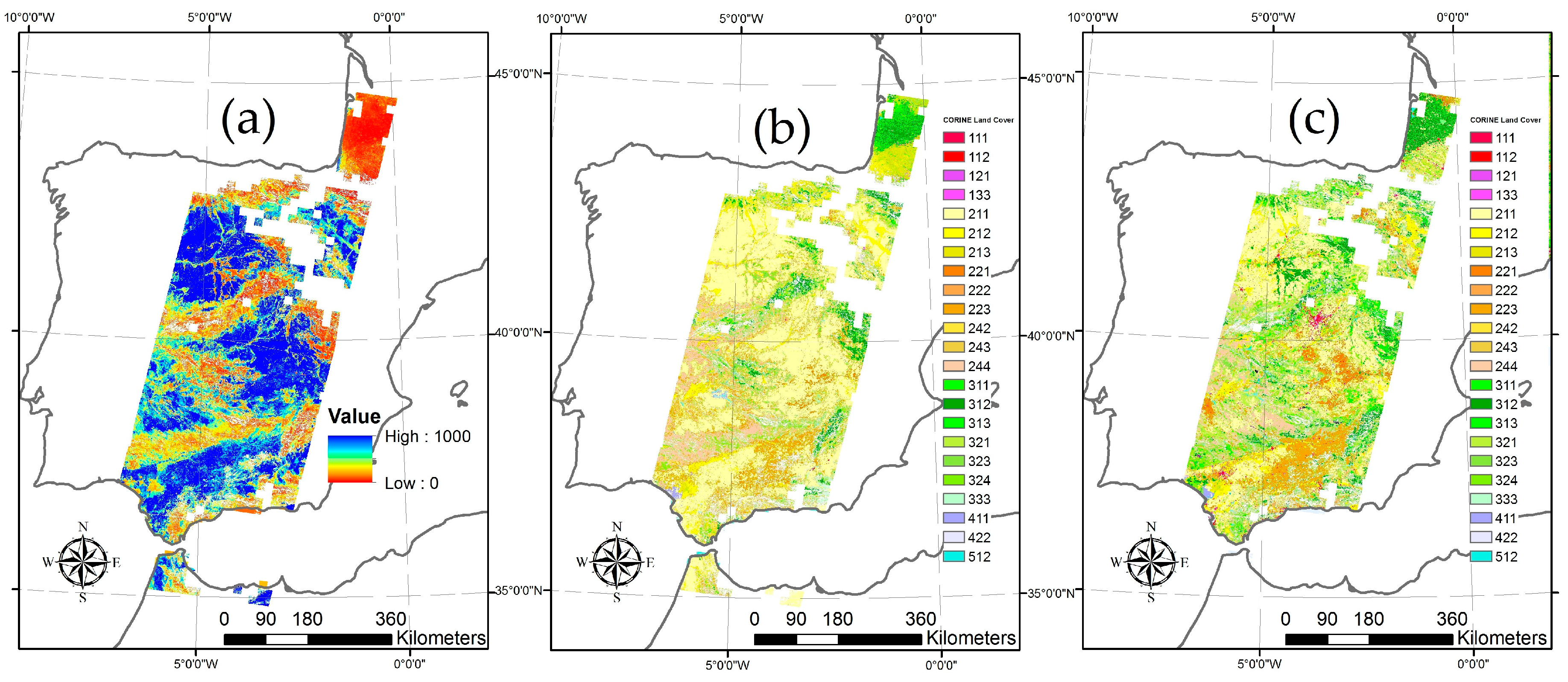
We obtained 23 classified maps and 23 × 7 confusion matrices. As can be seen in Figure 2, the general appearance is consistent with original CLC. Other examples are similar because broadly distributed classes are much better classified than others are.
The OA results according to the reclassification and assignment of the k-means classes to the CLC 2006 classes are shown in Table 2. The number of well-assigned pixels increased when both the number of k-means classes and the number of bands did (although when eight or nine bands were used, the results differ by cases). On the contrary, the values of OA decreased when the number of classes to differ increased, except for level 6, for which better results were obtained than Levels 4 and 5. There is a significant leap between levels 2 and 3.
The highest differences between consecutive levels were those found related to Levels 2 and 3. Levels 6 and 7 were the pair with the most variance of all the classifications performed (see Table 2). The pairs made up of Levels 1 and 2, and 4 and 5, are quite similar in all the classifications performed, while for the pair made up of Levels 5 and 6, the differences in the OA were the highest for the orbit 45320 classifications.
It seems remarkable that for Level 1 and Level 2, the percentage of pixels with a correct class assignation was higher than 90% in all cases, with scarce differences between factors. However, when we compared the last result with the more specific classifications, there were more considerable differences between using some bands, the number of classes, and the iterations. Furthermore, there were larger differences between those percentages and the assigned class variable.
Table 3 shows that kappa values decreased considerably concerning all the correctly classified pixels. Additionally, kappa values were positively correlated with the number of classes and number of bands. A large difference was observed in the most disaggregated classification, finding in some cases, very low kappa values. The differences between the kappa indices in Levels 4–5 and 5–6 are similar for all the experiments performed, with the exception of orbit 45320.
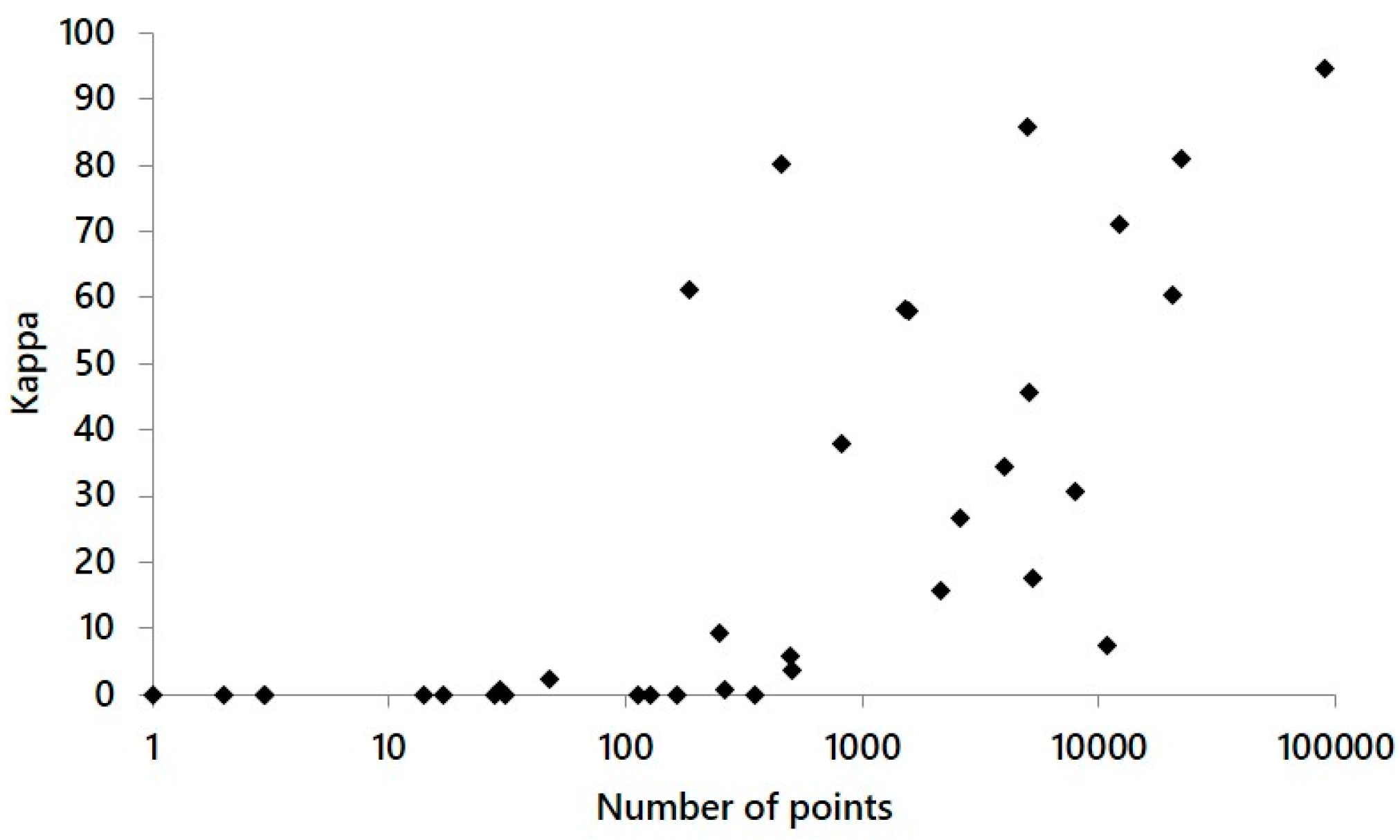
As Figure 3 suggests, there is a relationship between the total number of pixels belonging to a class and the kappa coefficient value. The classes with a low number of points had low kappa values (in many cases equal to zero). However, some classes had different kappa values than expected, namely classes 244, 312, 333, 411, 422, and 511. Table 4 summarizes the classification results (kappa and OA). Table 2, Table 3 and Table 4 show how kappa values are considerably smaller than OA values and that the results are not good enough for LULC classification.
It is important to highlight that the classes with average OA percentages higher than 70 were 211, 244, and 312. However, as can be seen in Table 5, other classes had good values of OA and kappa in some experiments (121, 212, 213, 333, and 422). It can also be seen that classes with a low number of CLC points usually have low accuracy values.
From all the confusion matrices (data not shown), it was possible to observe that the 211 category classified many points that were from other categories. Additionally, this confusion was more common in orbit 45320 than in the other one. The categories belonging to forest zones (311 to 334) could be better differentiated from the agricultural ones (211 to 244). However, grasslands (321) could not be differentiated from the agricultural categories in many cases. Urban categories (level 1 1) always showed a very low OA.
Moreover, the broad-leaved forest (311) category had poor classification results in general; we observed pixels from the 311 category classified in the same proportion as coniferous forest (312) or sclerophyllous vegetation (323).
The analyses of variance results for the first approach mentioned in the material and methods section are shown in Table 6. These results suggest that the factors band and classes are significant in most cases (p-value < 0.05). The number of iterations was only statistically significant in the highest level of disaggregation, whereas the orbit was significant for this maximum level of disaggregation and Levels 4 and 5.
Table 7 shows the global approach variance analyses performed, taking into account as another class the level, in addition to the bands, classes, iterations, and orbits. These results suggest that there are differences in the classification results by band, class, iteration, orbit, and the iteration between bands and levels. The Fisher statistical value (F value) was the highest for the levels’ categorical variable, followed by the classes used as an input in the k-means algorithm and bands.
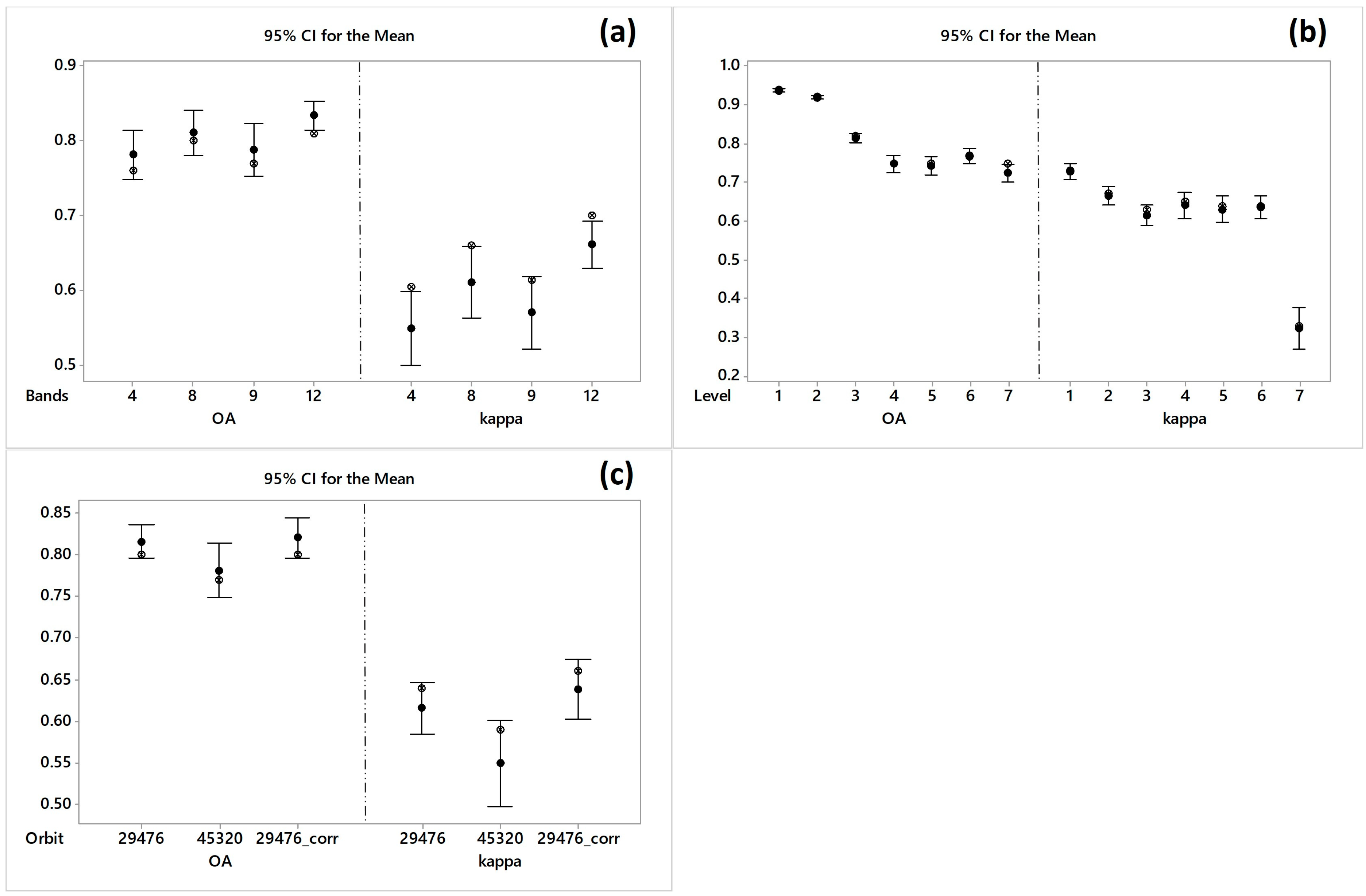
Figure 4, Figure 5 and Figure 6 show the results of the pairwise post hoc tests, in which we observe the differences between every group that built every factor or categorical variable.
It can be seen that the mean results of OA and kappa differ significantly (p-value < 0.05) between the experiments with nine and 12 bands, and between the experiments with four and 12 bands. Besides the classifications, the accuracy was better when we introduced the 12 bands than when we only introduced the multispectral information. Additionally, it is remarkable that we found lower OA and kappa coefficient values for the four MISR band experiments than for the other combinations of bands (see Figure 4a).
Figure 4b exhibits how in both the OA and kappa results, the values for Levels 1 and 2 were statistically higher than for the other levels. In Levels 3, 4, 5, and 6, the OA and kappa values were similar and different to those in Levels 1 and 2, and they were different to those of Level 7 (overall, those values achieved by the kappa).
Figure 4c shows that there were no statistically significant differences between the orbit classification accuracy for orbit 29476 and orbit 29476 (atmospherically corrected). The classification accuracy results for orbit 45320 were always slightly worse than those for orbit 29476 (see Figure 4c).
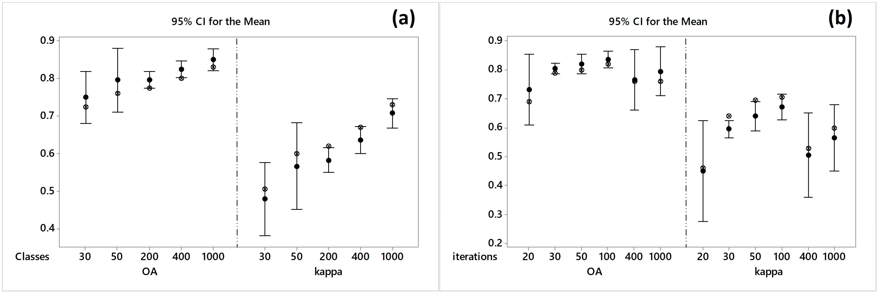
In general, better classification results were obtained when the number of classes for the k-means algorithm set was higher (see Figure 5a). Regarding the number of iterations, we inferred that the pairs made up of 30–100 iterations were the only pairs that differed significantly in the OA classification results. However, in the case of kappa coefficients, that pair of groups was also different and in addition to these, were those made up of 400–1000 and 100–1000 iterations. In these last two cases, the kappa coefficients were higher when we classified setting 100 iterations (reaching kappa values of 0.7) (see Figure 5b).
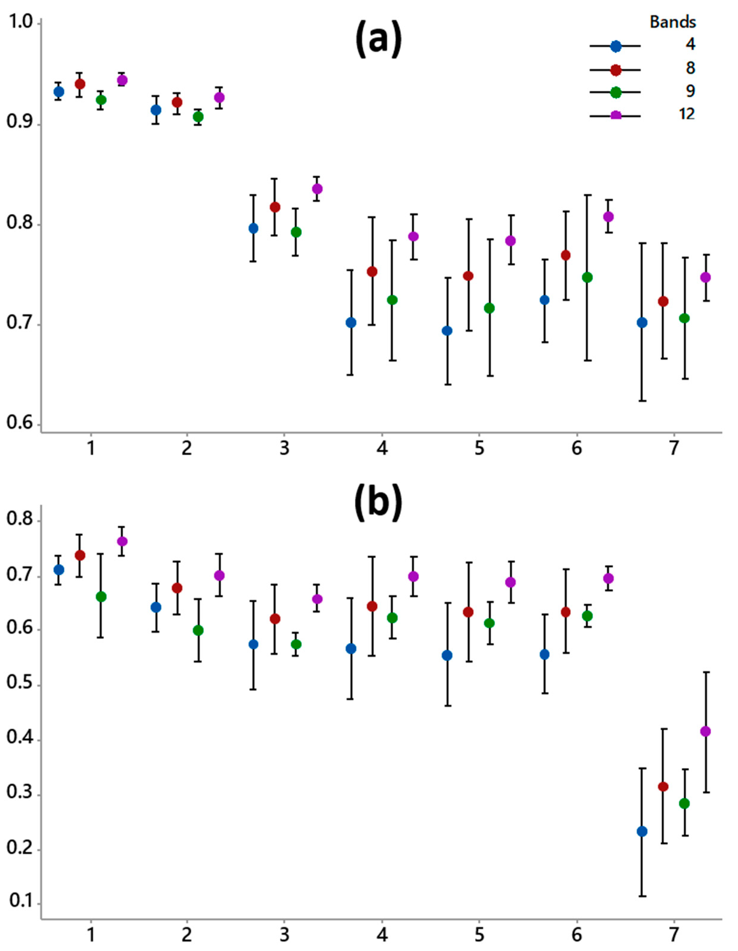
Figure 6 shows that the nine band category for Level 1 achieved the worst OA and kappa values (95% CI for the mean of band level) of all the band categories. For Level 2, the OA values for the nine band group were the worst of all the band groups, but this was not true for the kappa values. For Level 3, the OA nine band group values were similar to those achieved for the four band group category. On the other hand, in Levels 4, 5, 6, and 7, the nine band category OA and kappa values were higher than those for the four band group. Thereby, the only use of multiangular remote sensing information (nine bands) for the classifications yields worse results than the single purpose of multispectral data (four bands). Additionally, for all levels, the values of OA and kappa were higher when we used all available bands in the L1B2T MISR product (G-An, B-An, R-An, NIR-An, R-Bf, R-Af, R-Ba, R-Bf, R-Cf, R-Cf, R-Da y R-Df).
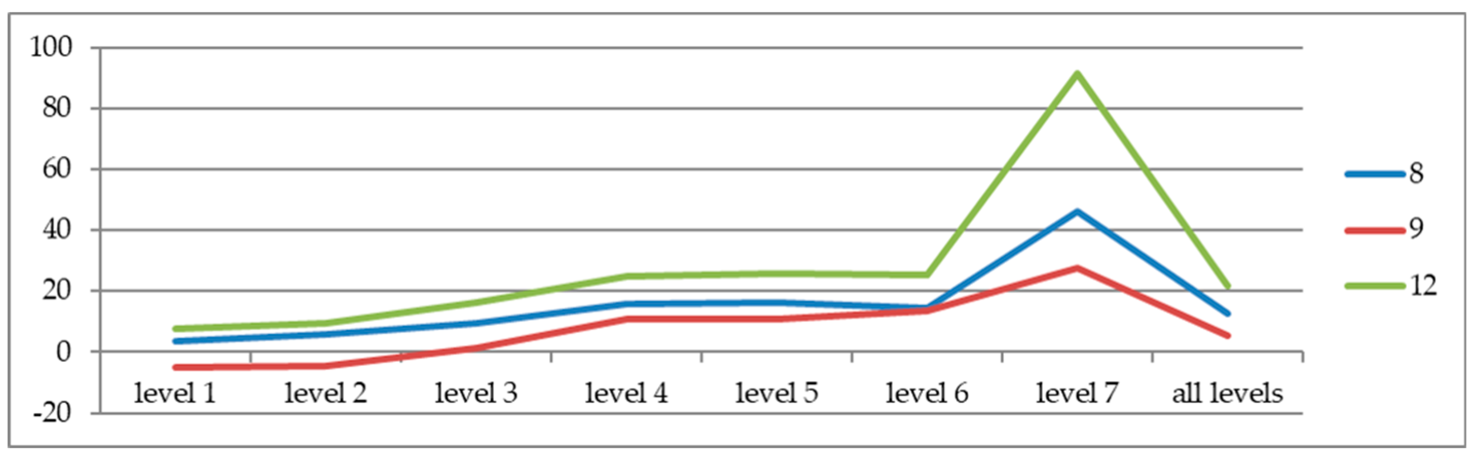
Figure 7 shows that adding more bands to four nadir bands (groups 8 and 12) improves the accuracy, with values from 3.7% (eight bands Level 1) to 91.3% (12 bands Level 7). It can be seen how relative improvements increase with Level 9 multiangular red bands; we obtained worse results (negative relative values) than for four nadir bands in Levels 1 and 2, but more desegregated classes did not occur. Additionally, four external bands improve the accuracy, concerning to eight-band improvements (see large differences between 8 and 12 bands).
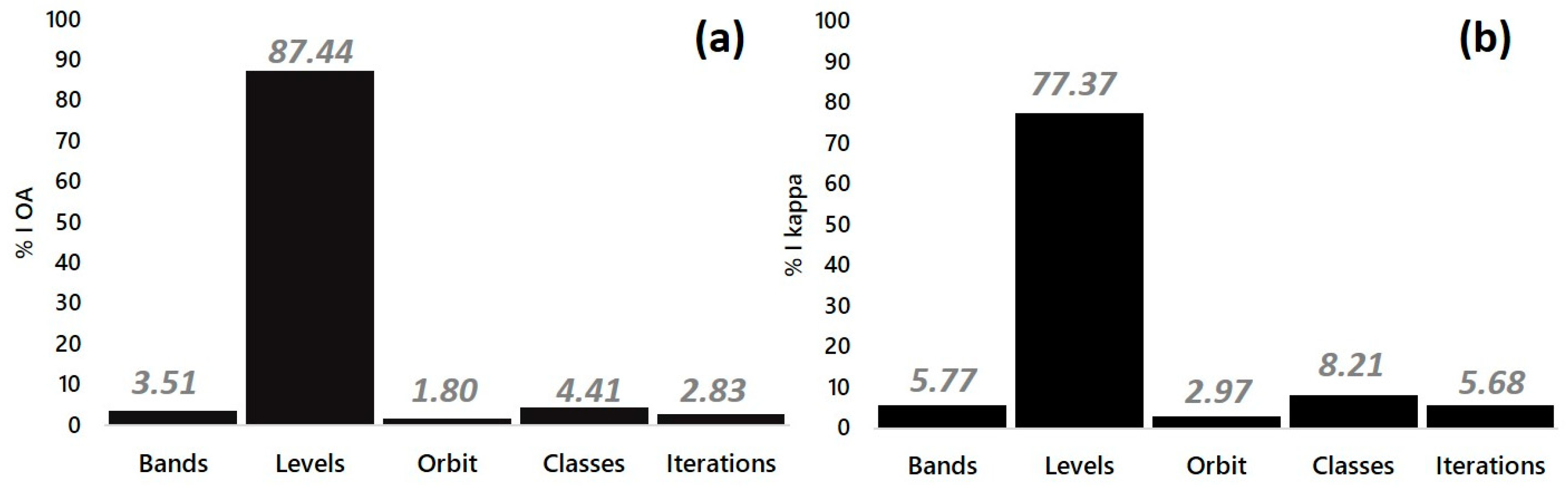
Figure 8 shows the results of the hierarchical partition test. These results suggest that the level is the variable that presented the highest independent contribution of the explained variables as a percentage of the total explained variance. The variables that followed the level were the classes used by the k-means process and the bands involved in the classification experiment. The orbit is the variable that contributes least to the total OA and kappa variance explained by band, level, orbit, class, and iterations. It is remarkable that class is the second variable that most variations of the reliability classification showed, and relatively, this variable explained almost 26% more variability than the band chosen. In the k-means algorithm, the class explained around 42% more information than the bands and nearly 45% more variability than the iterations also involved in the k-means algorithm.
4. Discussion
Overall, the classification experiments only achieved good results (OA values larger than 0.9) for Level 1 and Level 2. High OA values were observed for the low-level classification; however, kappa values for these levels were medium. Significant differences in the number of points per class explain discrepancies between OA values and kappa values. Some classes with low presence have low OA class values, such that kappa coefficients can be smaller than OA values. Table 5 shows that some classes (121, 212, 213, 333, and 422) have larger values in some classification results than the average value. Therefore, it can be seen that our unsupervised approach is dependent on the frequency of the land covers, probably due to the random selection of initial seeds. These results imply that a supervised method may be able to obtain betters results, even for low-frequency classes.
Furthermore, we must take into account the fact that CLC global accuracy is not applicable to all classes; some of them have medium or low values (133, 141, 222, 241, 332, 333, and 411), for example, [64] found that forest land covers can have medium accuracies.
Global accuracy results are comparable or better to those obtained by other studies; for example, classification using k-means for all of France with a 1 km spatial scale using SPOT/VEGETATION [65]. This example had as points to test the accuracy of several CLCs reclassified by the authors. It should be noted that, at the time of evaluating the results obtained in the present study, the classified images were all of the Iberian Peninsula; this implies that we have to take it into account when we classify the complexity of the Mediterranean zones and the climatic differences that predominate in our study area [66]. However, it is difficult to compare the several works that can be found on remote sensing classification experiments because we consider that as well as, or even more important than, the classification method, the spectral and spatial resolution employment to take care of the exercise are also the reference categories or types of structures. For instance, one comparable example is that carried out by [67]. The authors obtained OA results from 48% to 96% to classify eight types of rainforest in Africa, using some sensors with very different spatial and spectral resolutions. In this sense, our study also reflects two critical items that influence the final accuracy of classifications. The first one regards the number of classes that differ in the experiment, and the second one is related to how different those classes are. This last issue seems relevant at the time of the decision on whether to group different typologies or not. This last fact is visible in our study, in that we obtained better OA and kappa results in Level 6 than in Levels 4 and 5.
With regards to the effects of using multiangular information, the results were similar to those of the few studies which have also used multiangular information provided by remote sensing technologies. As we expected, adding multiangular data improved the classification accuracy. For instance, Brown de Colstoun et al. [68] found that the use of multiangular information from the POLDER sensor improved the OA by nearly 5% compared to only using multispectral information. In that study, the authors found that in some classes, the increase in the accuracy of the results was even higher in some specific classes, such as wooded savannas, pastures, and urban/built-up areas. Our results showed a relevant improvement for wooded savannas (agro-forestry in Spain), but not for urban areas or grasslands. In our study area, grasslands are not green during summer, except alpine pastures, such that they can be very similar to agricultural areas. Mahtab et al. [45] also obtained better results when they included multiangular data from the MISR sensor in addition to adding only multispectral information. They found that some classes that did not differ through the nadir MISR cameras information did vary due to multiangular MISR information. Su et al. [46] also used multiangular remote sensing information to classify land covers. They found increased values of OA rounding to 10 and 15 percent when they used multiangular information in addition to the multispectral isolated information.
However, we have observed that when the level of disaggregation of the classes is low, the multiangular information seems to produce noise in the classification results, and that it is better to use only multispectral data than only multiangular data for classification. Moreover, we found that when the level of disaggregation is high in the classification process, it is better to use only multiangular information than to use only multispectral information (see Figure 6 and Figure 7). This result matches the idea that anisotropy can be a source of confusion at the classification time for classes with different structural types in the same class; i.e., this anisotropy may, for instance, change the spectral signature of a forest due to the density, height, amount, and type of leaves [39,69,70]. Land cover anisotropy disperses the values of a specific class and allows structural information to be obtained [71] related to the type of cover that it must be differencing or allows the differentiation between homogeneous structures, such as olive fields or agro-forestry areas, as occurs in the present study.
The most remarkable differences in permanently irrigated land cover and water bodies that we could appreciate between two dates were caused by the fact that in the year 2008 (orbit 45320), there were irrigation restrictions and the water level in the reservoirs was very low in our study area. The date of the remote sensing information to classify may be an essential determinant of the ultimate precision of the classification experiments, as the multiangular information and the phenological time in the ecosystems change by season and between years [47]. The atmospheric correction made in the present study did not suggest any improvement in results.
5. Conclusions
This work investigated the benefit of using multiangular remotely sensed information for the classification of land cover across mainland Spain. The most important findings of this study are as follows:
- Adding multiangular data to spectral data improves the accuracy of land cover differentiation. The improvement increases as the levels of disaggregation increase.
- More external cameras add multiangular information that can almost double the accuracy improvement obtained without them.
- Having a very large number of clusters in unsupervised algorithms improves classifications even more than multiangular data. This effect, in addition to an automatic optimization method to label classes, can give an opportunity to achieve good results for unsupervised algorithms.
- The global accuracy results obtained in the present study were not good enough to accept classifications, with medium kappa values. In some cases, these results reached 90% of OA; however, kappa values are lower than 0.8. It is difficult to obtain good results with only one image, for a large and diverse area.
Author Contributions
C.J.N. conceived and designed the experiments; C.J.N. and P.A.-F. performed the experiments; C.J.N., P.A.-F., and R.R.-C. analyzed the data, wrote parts of the article, and revised and improved the article.
Funding
This research received no external funding.
Acknowledgments
These data were obtained from the NASA Langley Research Center Atmospheric Science Data Center. The authors would like to thank the National Aeronautics and Space Administration and the Copernicus Land Monitoring Service for images and data provided.
Conflicts of Interest
The authors declare no conflict of interest.
References
- Birdsey, R.; Angeles-Perez, G.; Kurz, W.A.; Lister, A.; Olguin, M.; Pan, Y.; Wayson, C.; Wilson, B.; Johnson, K. Approaches to monitoring changes in carbon stocks for REDD+. Carbon Manag. 2013, 4, 519–537. [Google Scholar] [CrossRef]
- Myneni, R.B.; Dong, J.; Tucker, C.J.; Kaufmann, R.K.; Kauppi, P.E.; Liski, J.; Zhou, L.; Alexeyev, V.; Hughes, M.K. A large carbon sink in the woody biomass of Northern forests. Proc. Natl. Acad. Sci. USA 2001, 98, 14784–14789. [Google Scholar] [CrossRef] [PubMed] [Green Version]
- Schwalm, C.R.; Williams, C.A.; Schaefer, K.; Baldocchi, D.; Black, T.A.; Goldstein, A.H.; Law, B.E.; Oechel, W.C.; Paw U, K.T.; Scott, R.L. Reduction in carbon uptake during turn of the century drought in western North America. Nat. Geosci. 2012, 5, 551. [Google Scholar] [CrossRef] [Green Version]
- Giustarini, L.; Hostache, R.; Matgen, P.; Schumann, G.J.P.; Bates, P.D.; Mason, D.C. A Change Detection Approach to Flood Mapping in Urban Areas Using TerraSAR-X. IEEE Trans. Geosci. Remote Sens. 2013, 51, 2417–2430. [Google Scholar] [CrossRef]
- Potapov, P.V.; Turubanova, S.A.; Tyukavina, A.; Krylov, A.M.; McCarty, J.L.; Radeloff, V.C.; Hansen, M.C. Eastern Europe’s forest cover dynamics from 1985 to 2012 quantified from the full Landsat archive. Remote Sens. Environ. 2015, 159, 28–43. [Google Scholar] [CrossRef]
- Myneni, R.B.; Yang, W.; Nemani, R.R.; Huete, A.R.; Dickinson, R.E.; Knyazikhin, Y.; Didan, K.; Fu, R.; Negrón Juárez, R.I.; Saatchi, S.S.; et al. Large seasonal swings in leaf area of Amazon rainforests. Proc. Natl. Acad. Sci. USA 2007, 104, 4820–4823. [Google Scholar] [CrossRef] [PubMed] [Green Version]
- Fialko, Y.; Sandwell, D.; Simons, M.; Rosen, P. Three-dimensional deformation caused by the Bam, Iran, earthquake and the origin of shallow slip deficit. Nature 2005, 435, 295–299. [Google Scholar] [CrossRef] [PubMed] [Green Version]
- Khatami, R.; Mountrakis, G. Implications of classification of methodological decisions in flooding analysis from Hurricane Katrina. Remote Sens. 2012, 4, 3877–3891. [Google Scholar] [CrossRef]
- Alcantara, C.; Kuemmerle, T.; Prishchepov, A.V.; Radeloff, V.C. Mapping abandoned agriculture with multi-temporal MODIS satellite data. Remote Sens. Environ. 2012, 124, 334–347. [Google Scholar] [CrossRef]
- Anderson, M.C.; Allen, R.G.; Morse, A.; Kustas, W.P. Use of Landsat thermal imagery in monitoring evapotranspiration and managing water resources. Remote Sens. Environ. 2012, 122, 50–65. [Google Scholar] [CrossRef]
- Hong, B.; Limburg, K.E.; Hall, M.H.; Mountrakis, G.; Groffman, P.M.; Hyde, K.; Luo, L.; Kelly, V.R.; Myers, S.J. An integrated monitoring/modeling framework for assessing human–nature interactions in urbanizing watersheds: Wappinger and Onondaga Creek watersheds, New York, USA. Environ. Model. Softw. 2012, 32, 1–15. [Google Scholar] [CrossRef]
- Ogilvie, A.; Belaud, G.; Delenne, C.; Bailly, J.-S.P.; Bader, J.-C.; Oleksiak, A.L.; Ferry, L.; Martin, D. Decadal monitoring of the Niger Inner Delta flood dynamics using MODIS optical data. J. Hydrol. 2015, 523, 368–383. [Google Scholar] [CrossRef]
- Keegan, K.M.; Albert, M.R.; McConnell, J.R.; Baker, I. Climate change and forest fires synergistically drive widespread melt events of the Greenland Ice Sheet. Proc. Natl. Acad. Sci. USA 2014, 111, 7964–7967. [Google Scholar] [CrossRef] [PubMed] [Green Version]
- Knyazikhin, Y.; Schull, M.A.; Stenberg, P.; Mõttus, M.; Rautiainen, M.; Yang, Y.; Marshak, A.; Carmona, P.L.; Kaufmann, R.K.; Lewis, P. Hyperspectral remote sensing of foliar nitrogen content. Proc. Natl. Acad. Sci. USA 2013, 110, E185–E192. [Google Scholar] [CrossRef] [PubMed]
- McMenamin, S.K.; Hadly, E.A.; Wright, C.K. Climatic change and wetland desiccation cause amphibian decline in Yellowstone National Park. Proc. Natl. Acad. Sci. USA 2008, 105, 16988–16993. [Google Scholar] [CrossRef] [PubMed]
- Syed, T.H.; Famiglietti, J.S.; Chambers, D.P.; Willis, J.K.; Hilburn, K. Satellite-based global-ocean mass balance estimates of interannual variability and emerging trends in continental freshwater discharge. Proc. Natl. Acad. Sci. USA 2010, 107, 17916–17921. [Google Scholar] [CrossRef] [PubMed] [Green Version]
- Asner, G.P.; Knapp, D.E.; Balaji, A.; Paez-Acosta, G. Automated mapping of tropical deforestation and forest degradation: CLASlite. J. Appl. Remote Sens. 2009, 3, 1–24. [Google Scholar] [CrossRef]
- Mendenhall, C.D.; Sekercioglu, C.H.; Brenes, F.O.; Ehrlich, P.R.; Daily, G.C. Predictive model for sustaining biodiversity in tropical countryside. Proc. Natl. Acad. Sci. USA 2013, 108, 16313–16316. [Google Scholar] [CrossRef] [PubMed]
- Nagendra, H.; Gadgil, M. Biodiversity assessment at multiple scales: Linking remote sensing data with field information. Proc. Natl. Acad. Sci. USA 1999, 96, 9154–9158. [Google Scholar] [CrossRef] [PubMed]
- Chuvieco, E. Teledetección ambiental: La observación de la tierra desde el espacio; Ariel: Barcelona, Spain, 2010. [Google Scholar]
- Eastman, J.R. IDRISI Kilimanjaro: Guide to GIS and Image Processing; Clark Labs, Clark University Worcester: Worcester, MA, USA, 2003. [Google Scholar]
- Yu, L.; Liang, L.; Wang, J.; Zhao, Y.; Cheng, Q.; Hu, L.; Liu, S.; Yu, L.; Wang, X.; Zhu, P. Meta-discoveries from a synthesis of satellite-based land-cover mapping research. Int. J. Remote Sens. 2014, 35, 4573–4588. [Google Scholar] [CrossRef] [Green Version]
- Martínez, B.; Gilabert, M.A. Vegetation dynamics from NDVI time series analysis using the wavelet transform. Remote Sens. Environ. 2009, 113, 1823–1842. [Google Scholar] [CrossRef]
- Hasmadi, M.; Pakhriazad, H.Z.; Shahrin, M.F. Evaluating supervised and unsupervised techniques for land cover mapping using remote sensing data. Geogr.-Malays. J. Soc. Space 2017, 5, 1–10. [Google Scholar]
- Summers, D.; Lewis, M.; Ostendorf, B.; Chittleborough, D. Visible near-infrared reflectance spectroscopy as a predictive indicator of soil properties. Ecol. Indic. 2011, 11, 123–131. [Google Scholar] [CrossRef]
- Su, L. Optimizing support vector machine learning for semi-arid vegetation mapping by using clustering analysis. ISPRS J. Photogramm. Remote Sens. 2009, 64, 407–413. [Google Scholar] [CrossRef]
- Mountrakis, G.; Im, J.; Ogole, C. Support vector machines in remote sensing: A review. ISPRS J. Photogramm. Remote Sens. 2011, 66, 247–259. [Google Scholar] [CrossRef]
- Lotsch, A.; Tian, Y.; Friedl, M.A.; Myneni, R.B. Land cover mapping in support of LAI and FPAR retrievals from EOS-MODIS and MISR: Classification methods and sensitivities to errors. Int. J. Remote Sens. 2003, 24, 1997–2016. [Google Scholar] [CrossRef]
- Nie, F.; Wang, H.; Huang, H.; Ding, C. Unsupervised and semi-supervised learning via ℓ 1-norm graph. In Proceedings of the 2011 IEEE International Conference on Computer Vision (ICCV), Barcelona, Spain, 6–13 November 2011; pp. 2268–2273. [Google Scholar]
- Cheng, G.; Han, J.; Lu, X. Remote Sensing Image Scene Classification: Benchmark and State of the Art. Proc. IEEE 2017, 105, 1865–1883. [Google Scholar] [CrossRef] [Green Version]
- Rozenstein, O.; Karnieli, A. Comparison of methods for land-use classification incorporating remote sensing and GIS inputs. Appl. Geogr. 2011, 31, 533–544. [Google Scholar] [CrossRef]
- San Miguel-Ayanz, J.; Biging, G.S. Comparison of single-stage and multi-stage classification approaches for cover type mapping with TM and SPOT data. Remote Sens. Environ. 1997, 59, 92–104. [Google Scholar] [CrossRef]
- Nicodemus, F.E.; Richmond, J.C.; Hsia, J.J.; Ginsberg, I.W.; Limperis, T. Geometrical Considerations and Nomenclature for Reflectance; US Department of Commerce, National Bureau of Standards: Washington, DC, USA, 1977; Volume 160, pp. 94–145.
- Diner, D.J.; Ackerman, T.P.; Braverman, A.J.; Bruegge, C.J.; Chopping, M.J.; Clothiaux, E.E.; Davies, R.; Di Girolamo, L.; Kahn, R.A.; Knyazikhin, Y.; et al. Ten years of MISR observations from Terra: Looking back, ahead, and in between. In Proceedings of the 2010 IEEE International Geoscience and Remote Sensing Symposium (IGARSS), Honolulu, HI, USA, 25–30 July 2010; pp. 1297–1299. [Google Scholar]
- Diner, D.J.; Braswell, B.H.; Davies, R.; Gobron, N.; Hu, J.; Jin, Y.; Kahn, R.A.; Knyazikhin, Y.; Loeb, N.; Muller, J.-P.; et al. The value of multiangle measurements for retrieving structurally and radiatively consistent properties of clouds, aerosols, and surfaces. Remote Sens. Environ. 2005, 97, 495–518. [Google Scholar] [CrossRef]
- Diner, D.J.; Martonchik, J.V.; Kahn, R.A.; Pinty, B.; Gobron, N.; Nelson, D.L.; Holben, B.N. Using angular and spectral shape similarity constraints to improve MISR aerosol and surface retrievals over land. Remote Sens. Environ. 2005, 94, 155. [Google Scholar] [CrossRef]
- Gobron, N.; Gobron, N.; Pinty, B.; Verstraete, M.M.; Widlowski, J.L.A.W.J.L.; Diner, D.J.A.D.D.J. Uniqueness of multiangular measurements. II. Joint retrieval of vegetation structure and photosynthetic activity from MISR. IEEE Trans. Geosci. Remote Sens. 2002, 40, 1574–1592. [Google Scholar] [CrossRef]
- Zhang, Y.; Shabanov, N.; Knyazikhin, Y.; Myneni, R.B. Assessing the information content of multiangle satellite data for mapping biomes II. Theory. Remote Sens. Environ. 2002, 80, 435–446. [Google Scholar] [CrossRef]
- Armston, J.D.; Scarth, P.F.; Phinn, S.R.; Danaher, T.J. Analysis of multi-date MISR measurements for forest and woodland communities, Queensland, Australia. Remote Sens. Environ. 2007, 107, 287–298. [Google Scholar] [CrossRef]
- Arrogante-Funes, P.; Novillo, C.J.; Romero-Calcerrada, R.; Vázquez-Jiménez, R.; Ramos-Bernal, R.N. Relationship between MRPV Model Parameters from MISRL2 Land Surface Product and Land Covers: A Case Study within Mainland Spain. ISPRS Int. J. Geo-Inf. 2017, 6, 353. [Google Scholar] [CrossRef]
- Abuelgasim, A.A.; Gopal, S.; Irons, J.R.; Strahler, A.H. Classification of ASAS multiangle and multispectral measurements using artificial neural networks. Remote Sens. Environ. 1996, 57, 79–87. [Google Scholar] [CrossRef]
- Hyman, A.H.; Barnsley, M.J. On the potential for land cover mapping from multiple-view-angle (MVA) remotely-sensed images. Int. J. Remote Sens. 1997, 18, 2471–2475. [Google Scholar] [CrossRef]
- Xavier, A.S.; Galvao, L.S. View angle effects on the discrimination of selected Amazonian land cover types from a principal-component analysis of MISR spectra. Int. J. Remote Sens. 2005, 26, 3797–3811. [Google Scholar] [CrossRef]
- Liesenberg, V.; GalvÃo, L.S.; Ponzoni, F.J. Variations in reflectance with seasonality and viewing geometry: Implications for classification of Brazilian savanna physiognomies with MISR/Terra data. Remote Sens. Environ. 2007, 107, 276–286. [Google Scholar] [CrossRef]
- Mahtab, A.; Sridhar, V.N.; Navalgund, R.R. Impact of Surface Anisotropy on Classification Accuracy of Selected Vegetation Classes: An Evaluation Using Multidate Multiangular MISR Data over Parts of Madhya Pradesh, India. IEEE Trans. Geosci. Remote Sens. 2008, 46, 250–258. [Google Scholar] [CrossRef]
- Su, L.; Chopping, M.J.; Rango, A.; Martonchik, J.V.; Peters, D.P.C. Support vector machines for recognition of semi-arid vegetation types using MISR multiangle imagery. Remote Sens. Environ. 2007, 107, 299–311. [Google Scholar] [CrossRef]
- Braswell, B.H.; Hagen, S.C.; Frolking, S.E.; Salas, W.A. A multivariable approach for mapping sub-pixel land cover distributions using MISR and MODIS: Application in the Brazilian Amazon region. Remote Sens. Environ. 2003, 87, 243–256. [Google Scholar] [CrossRef]
- Chopping, M.J.; Rango, A.; Havstad, K.M.; Schiebe, F.R.; Ritchie, J.C.; Schmugge, T.J.; French, A.N.; Su, L.; McKee, L.; Davis, M.R. Canopy attributes of desert grassland and transition communities derived from multiangular airborne imagery. Remote Sens. Environ. 2003, 85, 339–354. [Google Scholar] [CrossRef]
- Chopping, M.; Moisen, G.G.; Su, L.; Laliberte, A.; Rango, A.; Martonchik, J.V.; Peters, D.P.C. Large area mapping of southwestern forest crown cover, canopy height, and biomass using the NASA Multiangle Imaging Spectro-Radiometer. Remote Sens. Environ. 2008, 112, 2051–2063. [Google Scholar] [CrossRef] [Green Version]
- Chopping, M.; North, M.; Chen, J.; Schaaf, C.B.; Blair, J.B.; Martonchik, J.V.; Bull, M.A. Forest canopy cover and height from MISR in topographically complex southwestern US landscapes assessed with high quality reference data. IEEE J. Sel. Top. Appl. Earth Obs. Remote Sens. 2012, 5, 44–58. [Google Scholar] [CrossRef]
- Heiskanen, J. Tree cover and height estimation in the Fennoscandian tundra-taiga transition zone using multiangular MISR data. Remote Sens. Environ. 2006, 103, 97–114. [Google Scholar] [CrossRef]
- Hill, M.J.; Averill, C.; Jiao, Z.; Schaaf, C.B.; Armston, J.D. Relationship of MISR RPV parameters and MODIS BRDF shape indicators to surface vegetation patterns in an Australian tropical savanna. Can. J. Remote Sens. 2008, 34, S247–S267. [Google Scholar] [CrossRef]
- Nolin, A.W. Towards retrieval of forest cover density over snow from the multiangle Imaging SpectroRadiometer (MISR). Hydrol. Process. 2004, 18, 3623–3636. [Google Scholar] [CrossRef]
- Selkowitz, D.J. A comparison of multi-spectral, multi-angular, and multi-temporal remote sensing datasets for fractional shrub canopy mapping in Arctic Alaska. Remote Sens. Environ. 2010, 114, 1338–1352. [Google Scholar] [CrossRef]
- Su, L.; Huang, Y.; Chopping, M.J.; Rango, A.; Martonchik, J.V. An empirical study on the utility of BRDF model parameters and topographic parameters for mapping vegetation in a semi-arid region with MISR imagery. Int. J. Remote Sens. 2009, 30, 3463–3483. [Google Scholar] [CrossRef]
- Diner, D.J.; Beckert, J.C.; Reilly, T.H.; Bruegge, C.J.; Conel, J.E.; Kahn, R.A.; Martonchik, J.V.; Ackerman, T.P.; Davies, R.; Gerstl, S.A.W.; et al. multiangle Imaging SpectroRadiometer (MISR) instrument description and experiment overview. IEEE Trans. Geosci. Remote Sens. 1998, 36, 1072–1087. [Google Scholar] [CrossRef]
- EEA. CLC2006 Technical Guidelines; European Environment Agency: Cope, SC, USA, 2007. [Google Scholar]
- Büttner, G.; Maucha, G. The Thematic Accuracy of Corine Land Cover 200; Assessment Using LUCAS (Land Use/Cover Area Frame Statistical Survey); EEA Technical Report No 7/2006; European Environment Agency: Copenhagen, Denmark, 2006. [Google Scholar]
- Büttner, G.; Kosztra, B.; Maucha, G.; Pataki, R. Implementation and Achievements of CLC2006; Final Draft, ETC-LUSI; EEA Technical Report No 89; European Environment Agency: Copenhagen, Denmark, 2010. [Google Scholar]
- Sedano, F.; Lavergne, T.; Ibanez, L.M.; Gong, P. A neural network-based scheme coupled with the RPV model inversion package. Remote Sens. Environ. 2008, 112, 3271–3283. [Google Scholar] [CrossRef]
- Chopping, M.; Nolin, A.; Moisen, G.G.; Martonchik, J.V.; Bull, M. Forest canopy height from the Multiangle Imaging SpectroRadiometer (MISR) assessed with high resolution discrete return lidar. Remote Sens. Environ. 2009, 113, 2172–2185. [Google Scholar] [CrossRef] [Green Version]
- Provost, F.J.; Fawcett, T.; Kohavi, R. The case against accuracy estimation for comparing induction algorithms. In Proceedings of the ICML, Madison, WI, USA, 24–27 July 1998; pp. 445–453. [Google Scholar]
- Chevan, A.; Sutherland, M. Hierarchical partitioning. Am. Statist. 1991, 45, 90–96. [Google Scholar]
- Felicísimo, A.M.; Sánchez Gago, L.M. Thematic and spatial accuracy: A comparison of the Corine Land Cover with the Forestry Map of Spain. In Proceedings of the 5th AGILE Conference on Geographic Information Science, Palma de Mallorca, Spain, 25–27 April 2002; pp. 109–118. [Google Scholar]
- Han, K.-S.; Champeaux, J.-L.; Roujean, J.-L. A land cover classification product over France at 1 km resolution using SPOT4/VEGETATION data. Remote Sens. Environ. 2004, 92, 52–66. [Google Scholar] [CrossRef]
- Shoshany, M. Satellite remote sensing of natural Mediterranean vegetation: A review within an ecological context. Prog. Phys. Geogr. 2000, 24, 153–178. [Google Scholar] [CrossRef]
- Thenkabail, P.S.; Enclona, E.A.; Ashton, M.S.; Legg, C.; De Dieu, M.J. Hyperion, IKONOS, ALI, and ETM+ sensors in the study of African rainforests. Remote Sens. Environ. 2004, 90, 23–43. [Google Scholar] [CrossRef]
- Brown de Colstoun, E.C.; Walthall, C.L. Improving global scale land cover classifications with multi-directional POLDER data and a decision tree classifier. Remote Sens. Environ. 2006, 100, 474–485. [Google Scholar] [CrossRef]
- Durbha, S.S.; King, R.L.; Younan, N.H. Support vector machines regression for retrieval of leaf area index from multiangle imaging spectroradiometer. Remote Sens. Environ. 2007, 107, 348–361. [Google Scholar] [CrossRef]
- Verrelst, J.; Clevers, J.; Schaepman, M.E. Merging the Minnaert-k Parameter with Spectral Unmixing to Map Forest Heterogeneity with CHRIS/PROBA Data. IEEE Trans. Geosci. Remote Sens. 2010, 48, 4014–4022. [Google Scholar] [CrossRef] [Green Version]
- Asner, G.P.; Braswell, B.H.; Schimel, D.S.; Wessman, C.A. Ecological Research Needs from Multiangle Remote Sensing Data. Remote Sens. Environ. 1998, 63, 155–165. [Google Scholar] [CrossRef]
Figure 1.
MISR orbits used in this study after cloud masking. (a) Represents orbit 29476, belonging to path 201 and captured on 3 July 2005; (b) Represents orbit 45320, belonging to path 201 and captured on 25 July 2008.
Figure 1.
MISR orbits used in this study after cloud masking. (a) Represents orbit 29476, belonging to path 201 and captured on 3 July 2005; (b) Represents orbit 45320, belonging to path 201 and captured on 25 July 2008.

Figure 2.
Example of maps obtained by using orbit 29476 corrected atmospherically, for 1000 classes, 100 iterations, and 12 bands. (a) Classified map with k-means classes; (b) Labeled map after k-means class aggregation; (c) Original CORINE land cover map.
Figure 2.
Example of maps obtained by using orbit 29476 corrected atmospherically, for 1000 classes, 100 iterations, and 12 bands. (a) Classified map with k-means classes; (b) Labeled map after k-means class aggregation; (c) Original CORINE land cover map.

Figure 3.
The relationship between the kappa coefficient of each class for Level 7 and the number of points in the class. The horizontal axis is logarithmic. The data are means for the classifications of orbit 29476 with and without atmospheric correction.
Figure 3.
The relationship between the kappa coefficient of each class for Level 7 and the number of points in the class. The horizontal axis is logarithmic. The data are means for the classifications of orbit 29476 with and without atmospheric correction.

Figure 4.
Interval plots from the pairwise post hoc test after applying the global approach variance analyses. (a) OA and kappa interval plots by bands; (b) OA and kappa interval plots by level; (c) OA and kappa interval plots by orbit. The circle with a cross inside represents the median values.
Figure 4.
Interval plots from the pairwise post hoc test after applying the global approach variance analyses. (a) OA and kappa interval plots by bands; (b) OA and kappa interval plots by level; (c) OA and kappa interval plots by orbit. The circle with a cross inside represents the median values.

Figure 5.
Interval plots from the pairwise post hoc test after applying the global approach variance analyses. (a) OA and kappa interval plots by the number of classes for the k-means; (b) OA and kappa interval plots by the number of iterations for the k-means. The circle with a cross inside represents the median values.

Figure 6.
Interval plots from the pairwise post hoc test after applying the global approach variance analyses for the iteration between the level and band factors. (a) Results using OA as the numerical variable; (b) Results using kappa as the numerical variable.
Figure 6.
Interval plots from the pairwise post hoc test after applying the global approach variance analyses for the iteration between the level and band factors. (a) Results using OA as the numerical variable; (b) Results using kappa as the numerical variable.

Figure 7.
Line plots of relative percentage improvement concerning only nadir data (four bands) obtained for every disaggregation level.
Figure 7.
Line plots of relative percentage improvement concerning only nadir data (four bands) obtained for every disaggregation level.

Figure 8.
Bar plots of the independent contribution of the explained variables as a percentage of total explained variance. (a) Results using OA as the numerical variable; (b) Results using kappa as the numerical variable.
Figure 8.
Bar plots of the independent contribution of the explained variables as a percentage of total explained variance. (a) Results using OA as the numerical variable; (b) Results using kappa as the numerical variable.


Table 1.
CORINE Land Cover 2006 and the groups for every classification performed (L1, L2, L3, L4, L5, L6, and L7) in the present study.
Table 1.
CORINE Land Cover 2006 and the groups for every classification performed (L1, L2, L3, L4, L5, L6, and L7) in the present study.
| CORINE Level 1 | CORINE Level 2 | CORINE Level 3 | L1 | L2 | L3 | L4 | L5 | L6 | L7 |
|---|---|---|---|---|---|---|---|---|---|
| Artificial Surfaces | Urban fabric | Continuous urban fabric | 1 | 1 | 1 | 1 | 1 | 1 | 111 |
| Discontinuous urban fabric | 1 | 1 | 1 | 1 | 1 | 1 | 112 | ||
| Industrial, commercial and transport unit | Industrial or commercial units | 1 | 1 | 1 | 1 | 2 | 1 | 121 | |
| Port areas | 1 | 1 | 1 | 1 | 2 | 1 | 124 | ||
| Mine, dump and construction sites | Mineral extraction sites | 1 | 1 | 1 | 1 | 3 | 1 | 131 | |
| Dump sites | 1 | 1 | 1 | 1 | 3 | 1 | 132 | ||
| Construction sites | 1 | 1 | 1 | 1 | 3 | 1 | 133 | ||
| Artificial, non-agricultural vegetated areas | Green urban areas | 1 | 1 | 1 | 1 | 4 | 1 | 141 | |
| Sport and leisure facilities | 1 | 1 | 1 | 1 | 4 | 1 | 142 | ||
| Agricultural areas | Arable land | Non-irrigated arable land | 2 | 2 | 2 | 2 | 5 | 2 | 211 |
| Permanently irrigated land | 2 | 2 | 2 | 3 | 5 | 3 | 212 | ||
| Rice fields | 2 | 2 | 2 | 3 | 5 | 3 | 213 | ||
| Permanent crops | Vineyards | 2 | 2 | 2 | 4 | 6 | 4 | 221 | |
| Fruit trees and Berry plantations | 2 | 2 | 2 | 4 | 6 | 4 | 222 | ||
| Olive groves | 2 | 2 | 2 | 4 | 6 | 4 | 223 | ||
| Pastures | Pastures | 2 | 2 | 2 | 5 | 7 | 5 | 231 | |
| Heterogeneous agricultural areas | Annual crops associated with permanent crops | 2 | 2 | 3 | 6 | 8 | 6 | 241 | |
| Complex cultivation patterns | 2 | 2 | 3 | 6 | 8 | 6 | 242 | ||
| Land principally occupied by agriculture, with significant areas of natural vegetation | 2 | 2 | 3 | 6 | 8 | 6 | 243 | ||
| Agro-forestry areas | 2 | 2 | 3 | 6 | 8 | 6 | 244 | ||
| Forest and seminatural areas | Forests | Broad-leaved forest | 3 | 3 | 4 | 7 | 9 | 7 | 311 |
| Coniferous forest | 3 | 3 | 4 | 7 | 9 | 8 | 312 | ||
| Mixed forest | 3 | 3 | 4 | 7 | 9 | 9 | 313 | ||
| Scrub and/or herbaceous vegetation associations | Natural grasslands | 3 | 4 | 5 | 5 | 10 | 5 | 321 | |
| Moors and heathland | 3 | 4 | 5 | 8 | 10 | 10 | 322 | ||
| Sclerophyllous vegetation | 3 | 4 | 5 | 8 | 10 | 10 | 323 | ||
| Transitional Woodland-shrub | 3 | 4 | 5 | 8 | 10 | 10 | 324 | ||
| Open spaces with little or no vegetation | Beaches, dunes, sands | 3 | 4 | 6 | 8 | 11 | 10 | 331 | |
| Bare rocks | 3 | 4 | 6 | 8 | 11 | 10 | 332 | ||
| Sparsely vegetated areas | 3 | 4 | 6 | 8 | 11 | 10 | 333 | ||
| Burnt areas | 3 | 4 | 6 | 8 | 11 | 10 | 334 | ||
| Wetlands | Inland wetlands | Inland marshes | 4 | 5 | 7 | 9 | 12 | 11 | 411 |
| Maritime wetland | Salt marshes | 4 | 5 | 7 | 9 | 13 | 11 | 421 | |
| Salines | 4 | 5 | 7 | 9 | 13 | 11 | 422 | ||
| Water bodies | Water bodies | Water bodies | 5 | 5 | 7 | 9 | 14 | 11 | 512 |
Table 2.
OA classification results.
| Orbit | Class | Band | Iterations | Level 1 | Level 2 | Level 3 | Level 4 | Level 5 | Level 6 | Level 7 |
|---|---|---|---|---|---|---|---|---|---|---|
| 45320 | 30 | 4 | 20 | 0.92 | 0.9 | 0.76 | 0.64 | 0.63 | 0.69 | 0.59 |
| 200 | 4 | 30 | 0.93 | 0.91 | 0.78 | 0.67 | 0.66 | 0.72 | 0.63 | |
| 8 | 30 | 0.93 | 0.91 | 0.8 | 0.7 | 0.69 | 0.74 | 0.66 | ||
| 9 | 30 | 0.93 | 0.91 | 0.8 | 0.73 | 0.71 | 0.78 | 0.68 | ||
| 12 | 30 | 0.93 | 0.9 | 0.81 | 0.73 | 0.72 | 0.77 | 0.7 | ||
| 100 | 0.94 | 0.92 | 0.85 | 0.78 | 0.77 | 0.82 | 0.74 | |||
| 29476 | 30 | 4 | 400 | 0.93 | 0.9 | 0.77 | 0.67 | 0.66 | 0.67 | 0.76 |
| 50 | 8 | 1000 | 0.93 | 0.92 | 0.79 | 0.72 | 0.72 | 0.73 | 0.76 | |
| 200 | 4 | 100 | 0.94 | 0.92 | 0.81 | 0.73 | 0.73 | 0.74 | 0.76 | |
| 8 | 30 | 0.94 | 0.92 | 0.82 | 0.76 | 0.76 | 0.77 | 0.69 | ||
| 9 | 30 | 0.92 | 0.91 | 0.8 | 0.75 | 0.75 | 0.77 | 0.68 | ||
| 12 | 30 | 0.94 | 0.93 | 0.83 | 0.79 | 0.79 | 0.81 | 0.72 | ||
| 400 | 4 | 30 | 0.94 | 0.93 | 0.82 | 0.75 | 0.74 | 0.76 | 0.76 | |
| 12 | 50 | 0.95 | 0.93 | 0.84 | 0.8 | 0.8 | 0.81 | 0.76 | ||
| 1000 | 8 | 50 | 0.95 | 0.93 | 0.84 | 0.8 | 0.8 | 0.81 | 0.76 | |
| 12 | 100 | 0.95 | 0.94 | 0.85 | 0.81 | 0.81 | 0.83 | 0.78 | ||
| 29476 corr. | 200 | 9 | 50 | 0.93 | 0.9 | 0.77 | 0.67 | 0.66 | 0.67 | 0.76 |
| 400 | 4 | 30 | 0.94 | 0.93 | 0.84 | 0.76 | 0.75 | 0.77 | 0.72 | |
| 8 | 30 | 0.95 | 0.93 | 0.84 | 0.79 | 0.78 | 0.8 | 0.75 | ||
| 9 | 30 | 0.92 | 0.91 | 0.8 | 0.75 | 0.75 | 0.77 | 0.71 | ||
| 12 | 30 | 0.95 | 0.93 | 0.83 | 0.79 | 0.79 | 0.8 | 0.75 | ||
| 50 | 0.95 | 0.93 | 0.83 | 0.79 | 0.79 | 0.8 | 0.75 | |||
| 1000 | 12 | 100 | 0.95 | 0.94 | 0.85 | 0.82 | 0.81 | 0.83 | 0.78 |
Table 3.
Kappa coefficient classification results.
| Orbit | Class | Band | Iterations | Level 1 | Level 2 | Level 3 | Level 4 | Level 5 | Level 6 | Level 7 |
|---|---|---|---|---|---|---|---|---|---|---|
| 45320 | 30 | 4 | 20 | 0.68 | 0.6 | 0.46 | 0.44 | 0.43 | 0.47 | 0.08 |
| 200 | 4 | 30 | 0.7 | 0.63 | 0.53 | 0.51 | 0.49 | 0.54 | 0.14 | |
| 8 | 30 | 0.73 | 0.66 | 0.58 | 0.54 | 0.53 | 0.58 | 0.18 | ||
| 9 | 30 | 0.73 | 0.65 | 0.59 | 0.59 | 0.58 | 0.64 | 0.23 | ||
| 12 | 30 | 0.72 | 0.61 | 0.6 | 0.61 | 0.59 | 0.64 | 0.27 | ||
| 100 | 0.77 | 0.71 | 0.68 | 0.67 | 0.66 | 0.71 | 0.33 | |||
| 29476 | 30 | 4 | 400 | 0.69 | 0.59 | 0.54 | 0.53 | 0.52 | 0.49 | 0.18 |
| 50 | 8 | 1000 | 0.69 | 0.63 | 0.56 | 0.61 | 0.6 | 0.57 | 0.3 | |
| 200 | 4 | 100 | 0.72 | 0.67 | 0.62 | 0.62 | 0.61 | 0.6 | 0.31 | |
| 8 | 30 | 0.74 | 0.67 | 0.63 | 0.66 | 0.65 | 0.64 | 0.34 | ||
| 9 | 30 | 0.62 | 0.57 | 0.57 | 0.64 | 0.63 | 0.63 | 0.31 | ||
| 12 | 30 | 0.72 | 0.67 | 0.64 | 0.7 | 0.69 | 0.69 | 0.36 | ||
| 400 | 4 | 30 | 0.73 | 0.68 | 0.64 | 0.65 | 0.64 | 0.62 | 0.34 | |
| 12 | 50 | 0.77 | 0.71 | 0.67 | 0.72 | 0.71 | 0.7 | 0.38 | ||
| 1000 | 8 | 50 | 0.77 | 0.73 | 0.68 | 0.72 | 0.71 | 0.71 | 0.4 | |
| 12 | 100 | 0.79 | 0.74 | 0.68 | 0.74 | 0.73 | 0.72 | 0.62 | ||
| 29476 corr | 200 | 9 | 50 | 0.64 | 0.58 | 0.56 | 0.63 | 0.62 | 0.61 | 0.29 |
| 400 | 4 | 30 | 0.75 | 0.69 | 0.66 | 0.66 | 0.65 | 0.63 | 0.34 | |
| 8 | 30 | 0.76 | 0.71 | 0.66 | 0.7 | 0.69 | 0.68 | 0.36 | ||
| 9 | 30 | 0.67 | 0.61 | 0.58 | 0.64 | 0.63 | 0.63 | 0.31 | ||
| 12 | 30 | 0.77 | 0.71 | 0.65 | 0.71 | 0.7 | 0.69 | 0.37 | ||
| 50 | 0.77 | 0.71 | 0.66 | 0.7 | 0.7 | 0.69 | 0.37 | |||
| 1000 | 12 | 100 | 0.81 | 0.76 | 0.7 | 0.75 | 0.74 | 0.73 | 0.62 |
Table 4.
Summary of the classification results by level.
| Average | Maximum | Minimum | ||||
|---|---|---|---|---|---|---|
| Classification | OA | Kappa | OA | Kappa | OA | Kappa |
| Level 1 | 0.94 | 0.73 | 0.95 | 0.81 | 0.92 | 0.62 |
| Level 2 | 0.92 | 0.66 | 0.94 | 0.76 | 0.9 | 0.57 |
| Level 3 | 0.81 | 0.61 | 0.85 | 0.7 | 0.76 | 0.46 |
| Level 4 | 0.75 | 0.63 | 0.82 | 0.75 | 0.64 | 0.44 |
| Level 5 | 0.74 | 0.62 | 0.81 | 0.74 | 0.63 | 0.43 |
| Level 6 | 0.78 | 0.63 | 0.83 | 0.73 | 0.69 | 0.47 |
| Level 7 | 0.7 | 0.31 | 0.78 | 0.62 | 0.59 | 0.08 |
Table 5.
Mean and maximum of all experiments for OA and kappa for Level 7 classifications.
| CORINE Land Cover Class | Average OA | Maximum OA | Average Kappa | Maximum Kappa | Number of Land Cover Points |
|---|---|---|---|---|---|
| 111 | 0.11 | 0.55 | 0.03 | 0.41 | 252 |
| 112 | 0.00 | 0.07 | −0.01 | 0.00 | 278 |
| 121 | 0.16 | 0.84 | 0.12 | 0.79 | 31 |
| 124 | 0.00 | 0.00 | 0.00 | 0.00 | 128 |
| 131 | 0.01 | 0.13 | 0.00 | 0.03 | 54 |
| 132 | 0.00 | 0.02 | 0.00 | 0.00 | 3 |
| 133 | 0.01 | 0.17 | 0.00 | 0.05 | 24 |
| 141 | 0.00 | 0.00 | 0.00 | 0.00 | 28 |
| 142 | 0.00 | 0.00 | 0.00 | 0.00 | 3 |
| 211 | 0.90 | 0.98 | 0.92 | 0.96 | 108745 |
| 212 | 0.51 | 0.80 | 0.43 | 0.73 | 12539 |
| 213 | 0.39 | 0.84 | 0.31 | 0.79 | 1510 |
| 221 | 0.27 | 0.62 | 0.14 | 0.50 | 5959 |
| 222 | 0.02 | 0.28 | −0.01 | 0.08 | 628 |
| 223 | 0.58 | 0.86 | 0.50 | 0.82 | 21517 |
| 231 | 0.00 | 0.00 | 0.00 | 0.00 | 361 |
| 241 | 0.00 | 0.00 | 0.00 | 0.00 | 164 |
| 242 | 0.09 | 0.33 | −0.04 | 0.14 | 11951 |
| 243 | 0.09 | 0.30 | 0.00 | 0.09 | 3098 |
| 244 | 0.75 | 0.89 | 0.72 | 0.86 | 22547 |
| 311 | 0.27 | 0.66 | 0.13 | 0.55 | 4334 |
| 312 | 0.82 | 0.97 | 0.80 | 0.96 | 6900 |
| 313 | 0.04 | 0.31 | 0.00 | 0.10 | 1162 |
| 321 | 0.19 | 0.54 | 0.07 | 0.39 | 8432 |
| 322 | 0.10 | 0.58 | 0.00 | 0.00 | 20 |
| 323 | 0.30 | 0.59 | 0.30 | 0.46 | 6761 |
| 324 | 0.32 | 0.58 | 0.10 | 0.37 | 5371 |
| 331 | 0.17 | 1.00 | 0.09 | 1.00 | 2 |
| 332 | 0.00 | 0.00 | 0.00 | 0.00 | 82 |
| 333 | 0.37 | 0.81 | 0.34 | 0.76 | 2025 |
| 334 | 0.09 | 0.74 | 0.00 | 0.00 | 125 |
| 411 | 0.14 | 0.64 | 0.18 | 0.53 | 811 |
| 421 | 0.07 | 0.64 | 0.00 | 0.00 | 23 |
| 422 | 0.28 | 0.91 | 0.40 | 0.89 | 188 |
| 512 | 0.68 | 1.00 | 0.72 | 1.00 | 482 |
Table 6.
Results of the variance analyses performed by level (OA and k as numerical variables in every case). The asterisk (*) implies significant results with p-value < 0.05.
Table 6.
Results of the variance analyses performed by level (OA and k as numerical variables in every case). The asterisk (*) implies significant results with p-value < 0.05.
| Band | Class | Iterations | Orbit | |||||
|---|---|---|---|---|---|---|---|---|
| Level | OA | K | OA | K | OA | K | OA | K |
| 1 | * | * | * | * | ||||
| 2 | * | * | * | |||||
| 3 | * | * | * | |||||
| 4 | * | * | * | * | * | |||
| 5 | * | * | * | * | * | |||
| 6 | * | * | * | |||||
| 7 | * | * | * | * | * | * | ||
Table 7.
Results from the global approach variance analyses performed (OA and k as numerical variables in every case). The asterisk (*) implies significant results with p-value < 0.05. F is the Fisher statistical value.
Table 7.
Results from the global approach variance analyses performed (OA and k as numerical variables in every case). The asterisk (*) implies significant results with p-value < 0.05. F is the Fisher statistical value.
| Variables | OA | Kappa | ||||||
|---|---|---|---|---|---|---|---|---|
| Df | F value | Pr(>F) | Sig | Df | F Value | Pr(>F) | Sig | |
| Bands | 3 | 13.274 | 1.4 × 10⁻⁷ | * | 3 | 18.736 | 4.36 × 10⁻¹⁰ | * |
| Classes | 4 | 14.915 | 5.6 × 10⁻¹⁰ | * | 4 | 29.519 | <2.2 × 10⁻¹⁶ | * |
| Iterations | 3 | 3.813 | 1.2 × 10⁻² | * | 3 | 4.546 | 0.004659 | * |
| Levels | 6 | 309.435 | <2.2 × 10⁻¹⁶ | * | 6 | 268.126 | <2.2 × 10⁻¹⁶ | * |
| Orbits | 2 | 7.621 | 7.6 × 10⁻⁴ | * | 2 | 8.468 | 0.000357 | * |
| Bands:Levels | 18 | 2.426 | 2.3 × 10⁻³ | * | 18 | 2.412 | 0.002413 | * |
© 2018 by the authors. Licensee MDPI, Basel, Switzerland. This article is an open access article distributed under the terms and conditions of the Creative Commons Attribution (CC BY) license (http://creativecommons.org/licenses/by/4.0/).
Share and Cite
MDPI and ACS Style
Novillo, C.J.; Arrogante-Funes, P.; Romero-Calcerrada, R. Improving Land Cover Classifications with Multiangular Data: MISR Data in Mainland Spain. Remote Sens. 2018, 10, 1717. https://0-doi-org.brum.beds.ac.uk/10.3390/rs10111717
AMA Style
Novillo CJ, Arrogante-Funes P, Romero-Calcerrada R. Improving Land Cover Classifications with Multiangular Data: MISR Data in Mainland Spain. Remote Sensing. 2018; 10(11):1717. https://0-doi-org.brum.beds.ac.uk/10.3390/rs10111717
Chicago/Turabian StyleNovillo, Carlos J., Patricia Arrogante-Funes, and Raúl Romero-Calcerrada. 2018. "Improving Land Cover Classifications with Multiangular Data: MISR Data in Mainland Spain" Remote Sensing 10, no. 11: 1717. https://0-doi-org.brum.beds.ac.uk/10.3390/rs10111717
Note that from the first issue of 2016, this journal uses article numbers instead of page numbers. See further details here.