Multi-Temporal Loess Landslide Inventory Mapping with C-, X- and L-Band SAR Datasets—A Case Study of Heifangtai Loess Landslides, China

 ,
, 
Abstract
:
1. Introduction
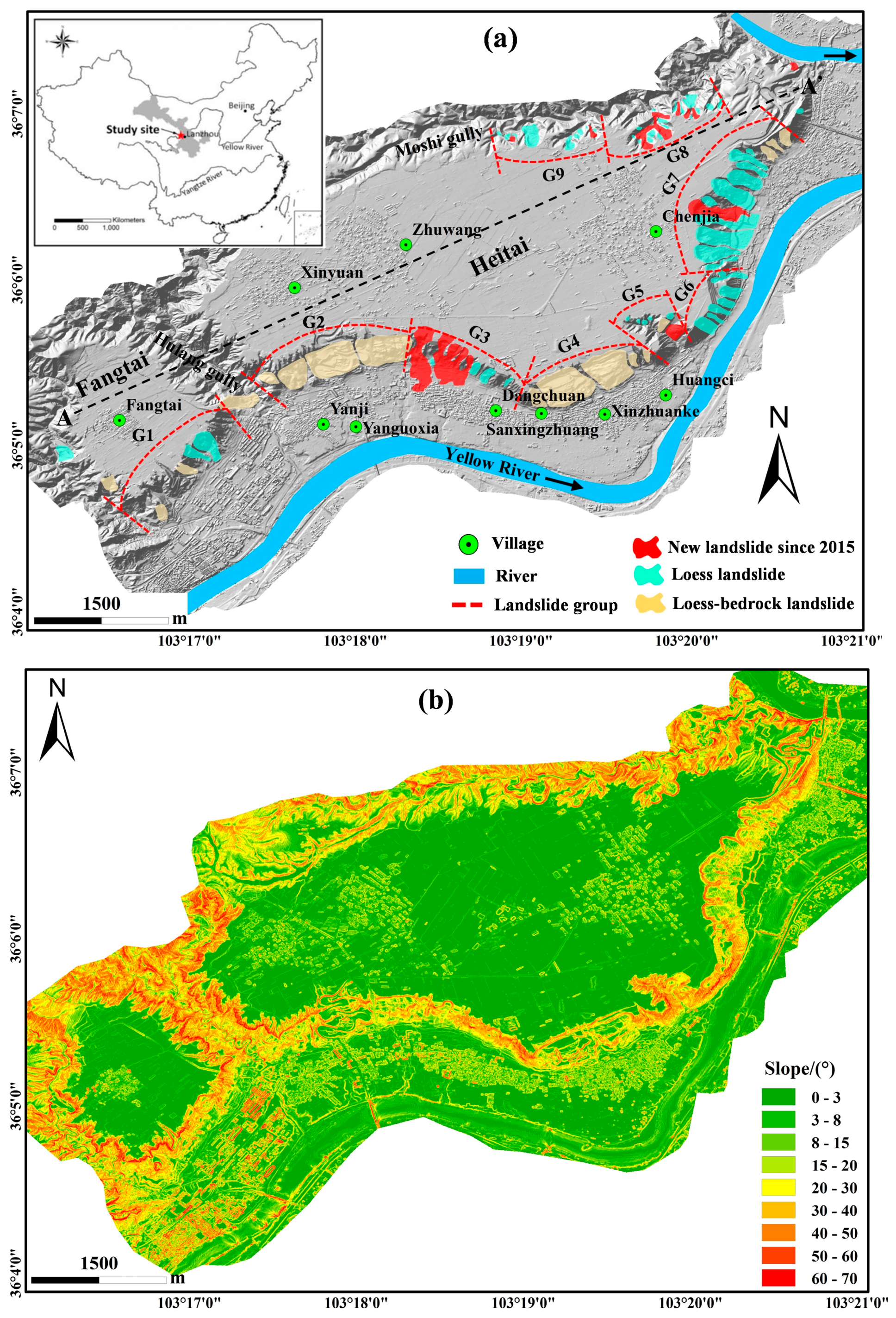
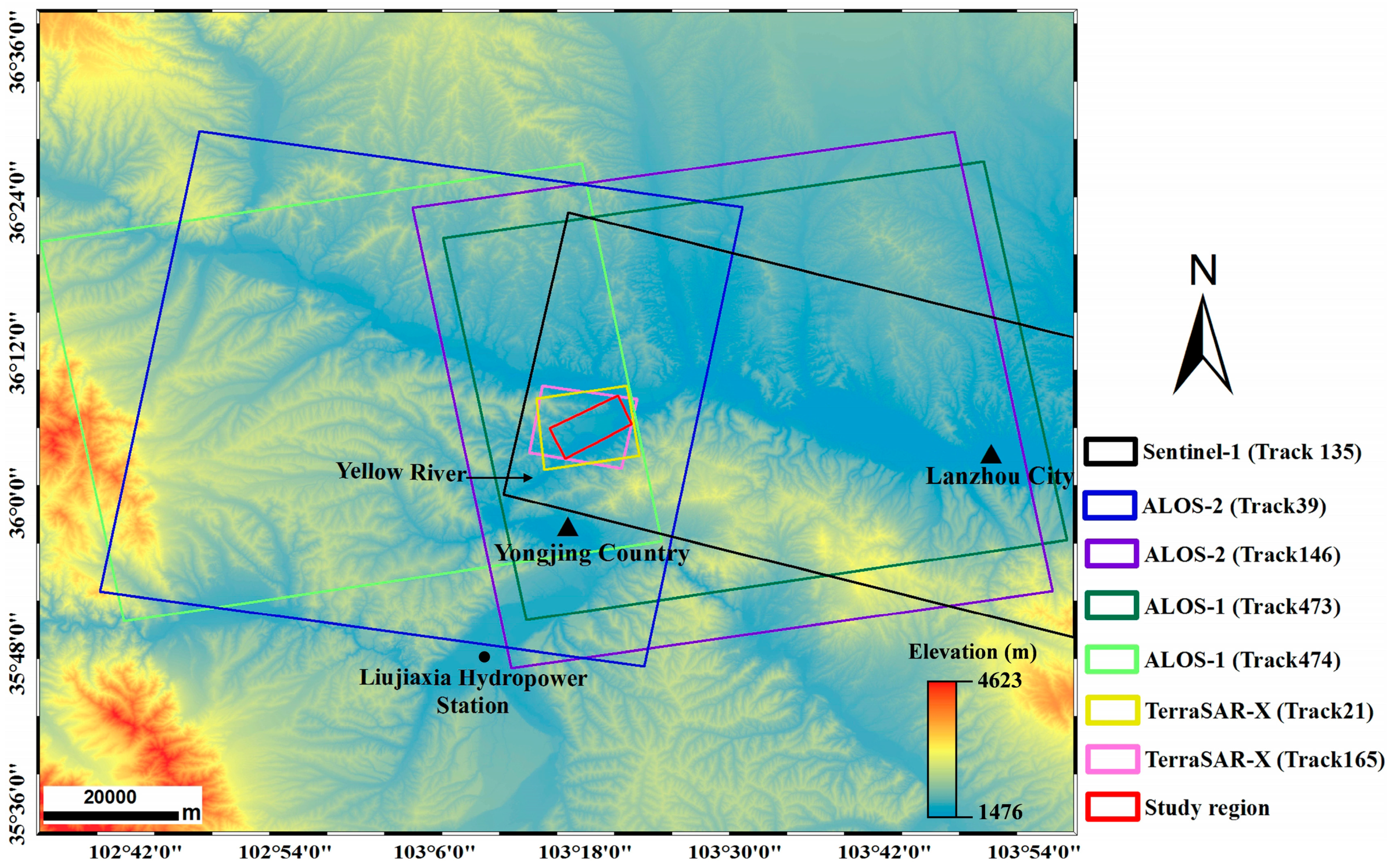
2. The Study Area
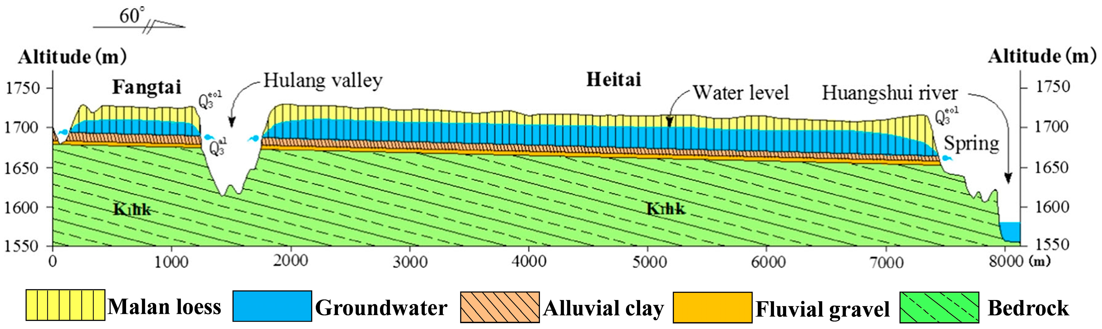
2.1. Geological Setting
2.2. Landslides
3. Datasets and Methodology
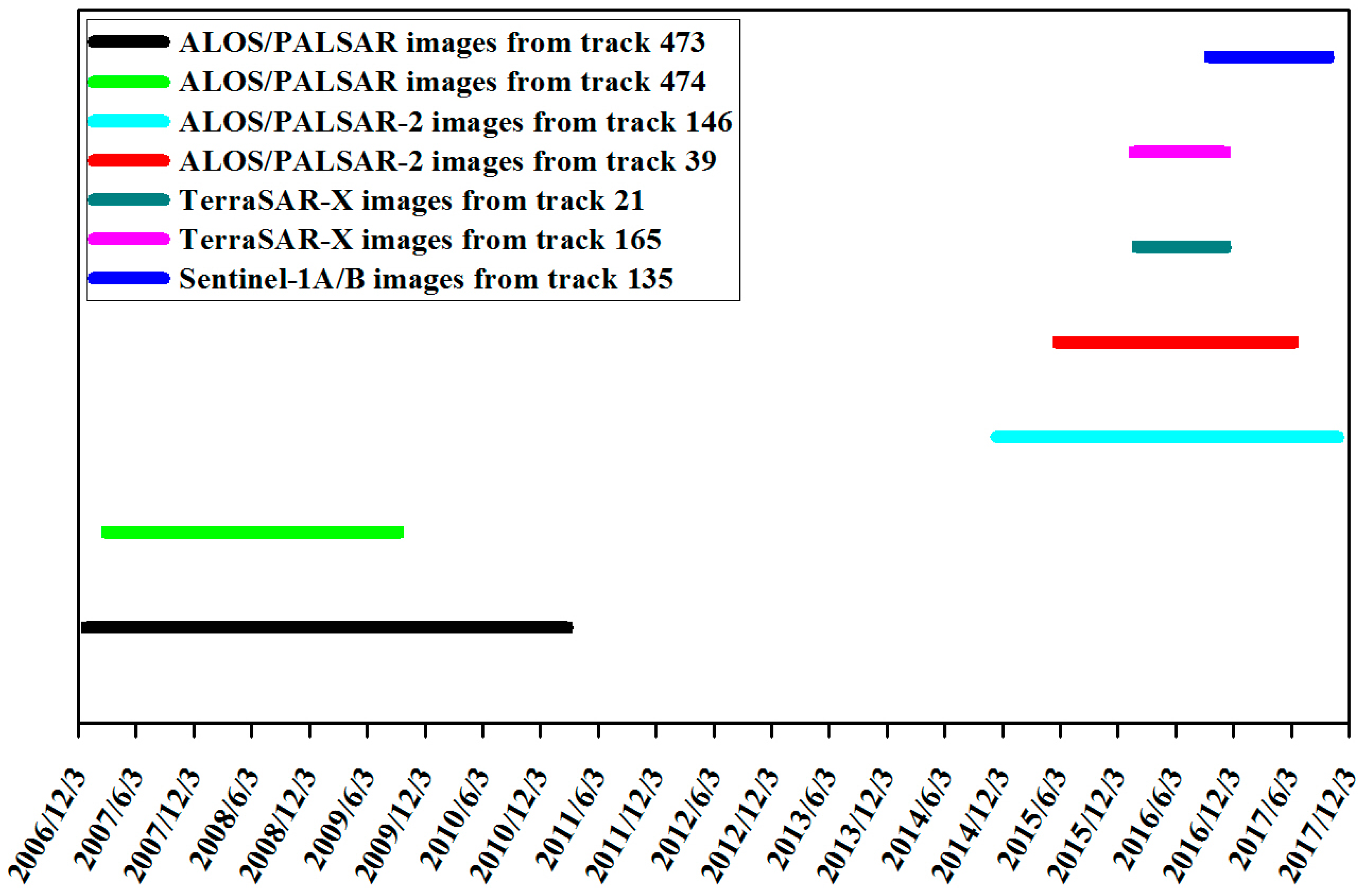
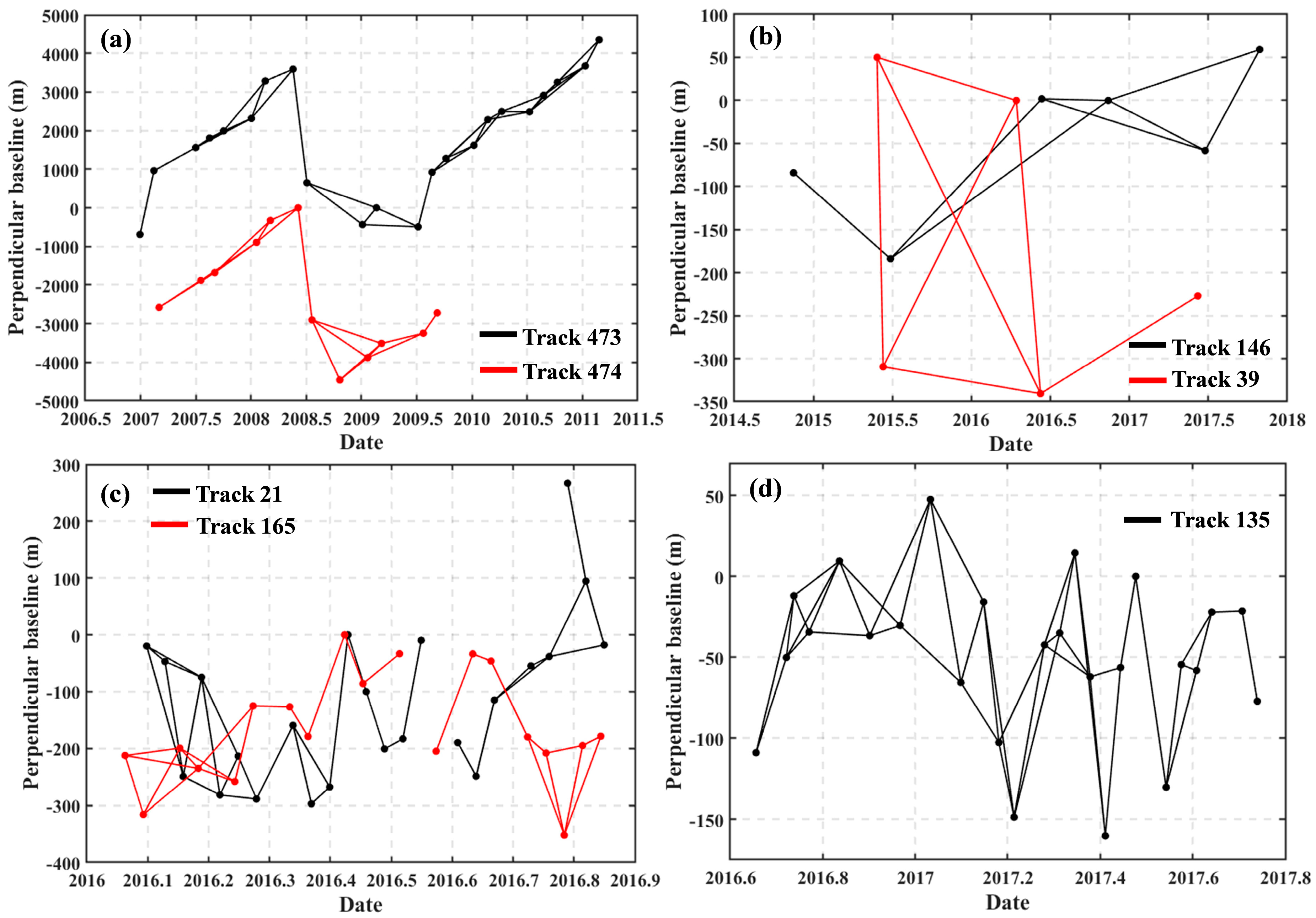
3.1. Datasets
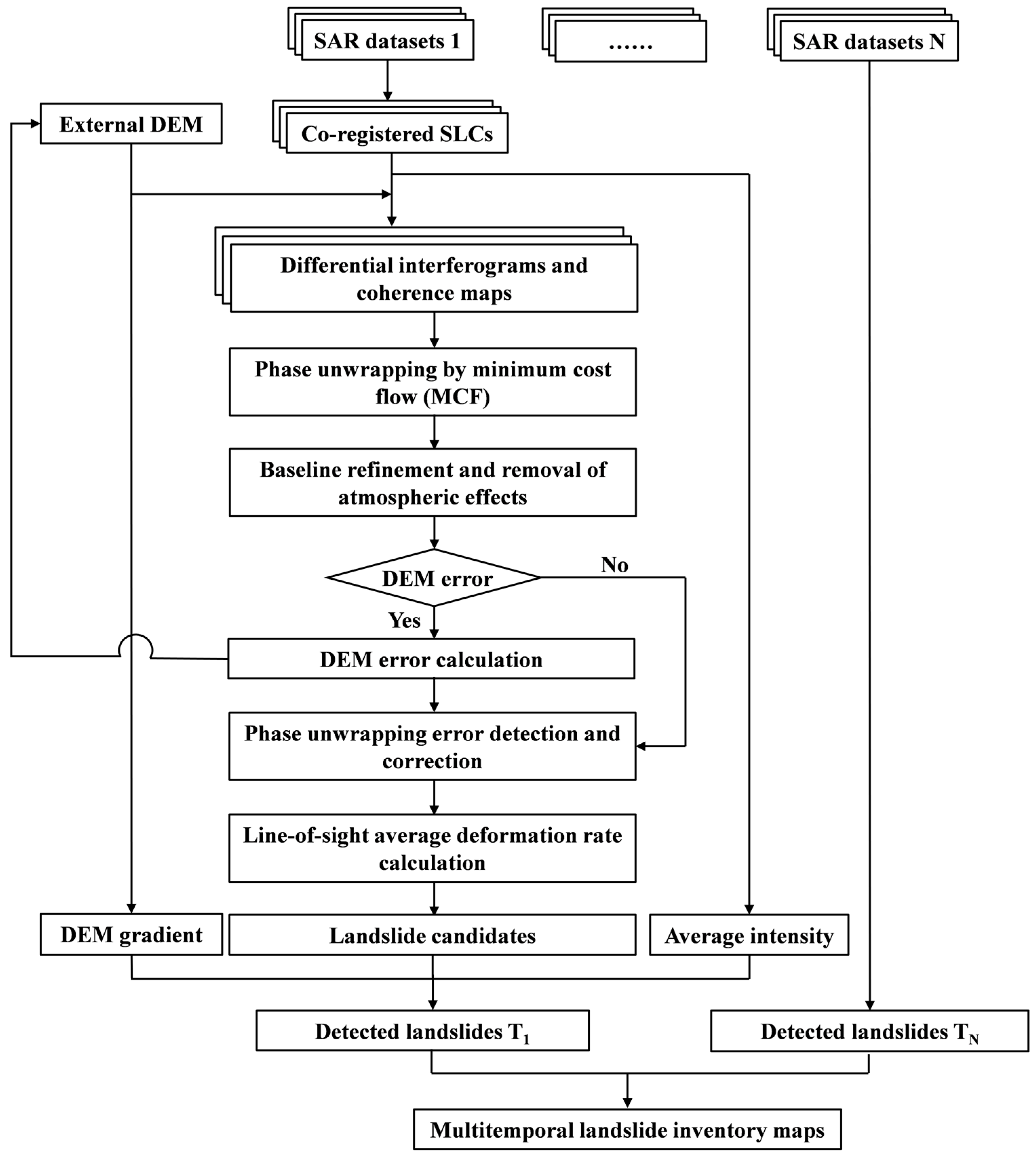
3.2. Flowchart of Landslide Identification with the InSAR Method
3.3. DEM Error Correction
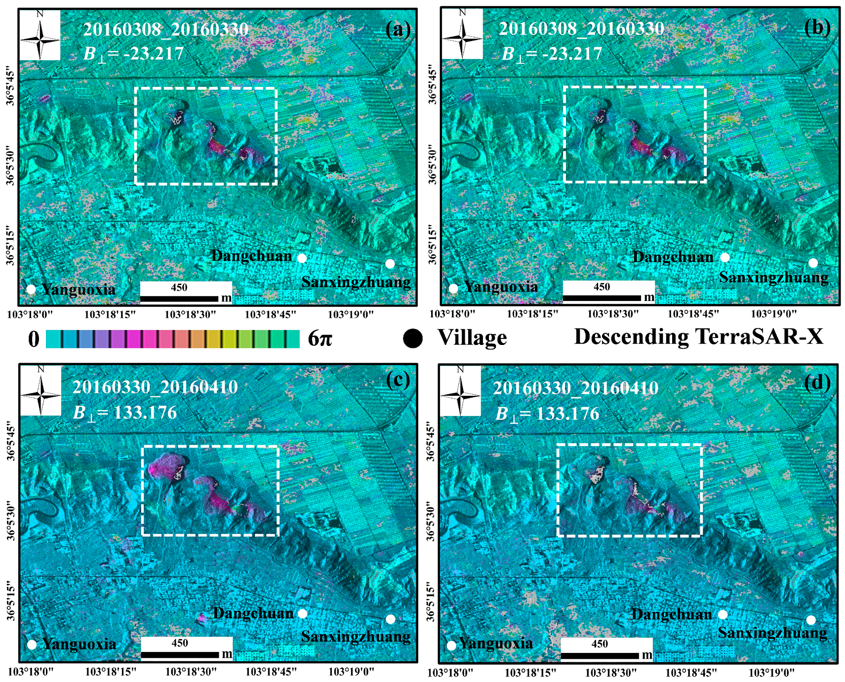
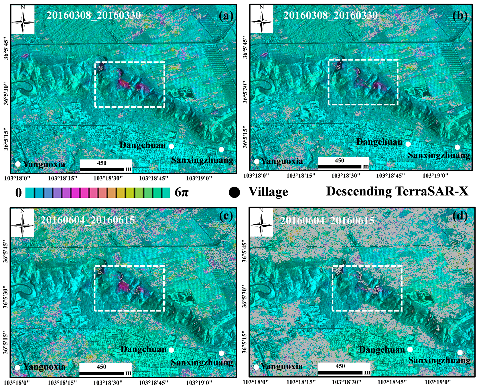
3.4. Phase Unwrapping Error Detection and Correction
4. Results
4.1. Error Detection and Correction
4.1.1. DEM Error Correction
4.1.2. Phase Unwrapping Error Correction
4.2. Identification of Potential Landslides
- (i)
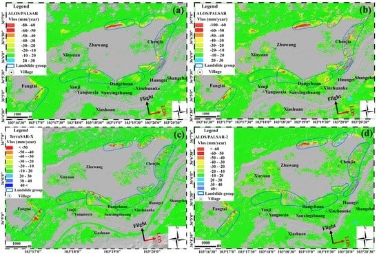
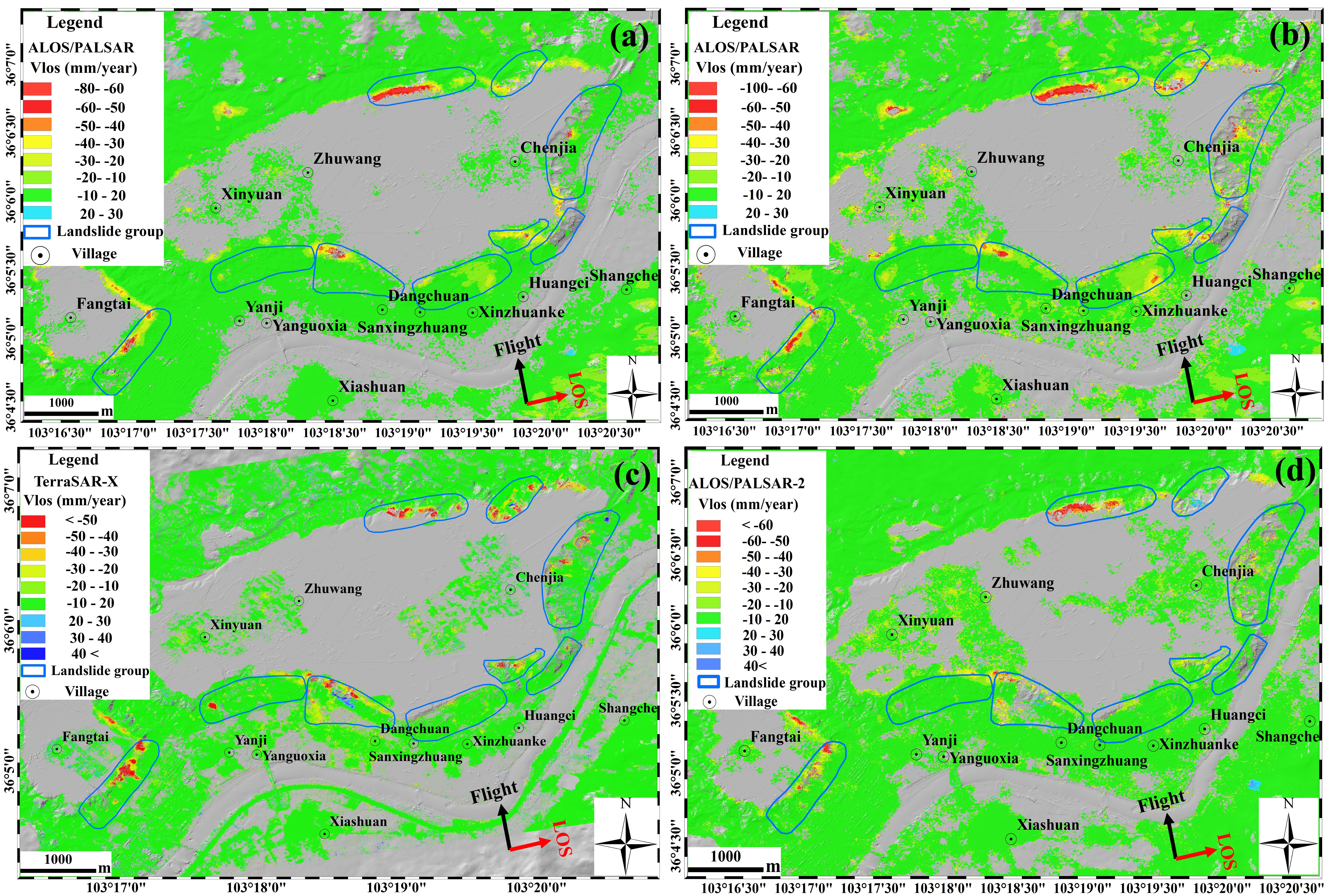
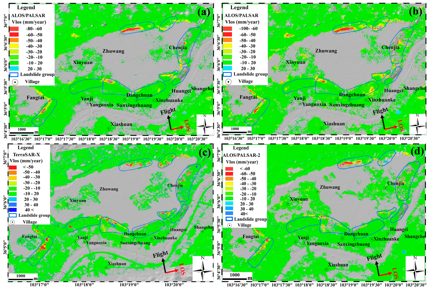
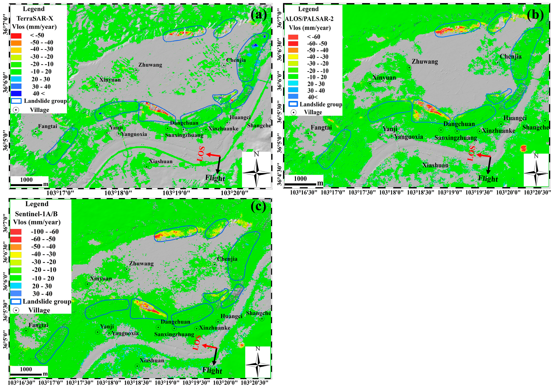
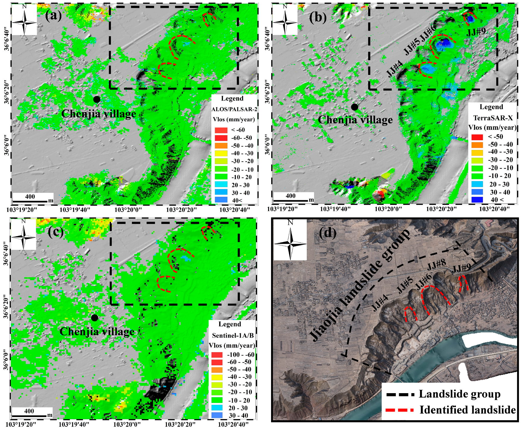
- It can be seen from Figure 9 and Figure 10 that the deformation regions calculated with different SAR datasets during a similar period are in good overall agreement, meaning that slow-rate surface deformation can be measured by different SAR data once it can be mapped in the line-of-sight direction. Furthermore, the existence of differences among different SAR datasets are mainly caused by different SAR acquisition parameters, including SAR acquisition date, wavelength, spatial resolution, local incidence angle and satellite tracking direction, which can be used to obtain more detailed information on each individual landslide.
- (ii)
- The deformation region of the Heifangtai terrace before 2011 was significantly different than that after 2014. From December 2006 to March 2011, the deformation regions of the Heifangtai terrace were mainly concentrated in the Fangtai, Yehugou and Moshigou landslide groups. However, after 2014, the main deformation region extended to Dangchuan landslide group, where large deformation occurred. Furthermore, some new deformation regions developed in the Xinyuan, Jiaojia and Chenjia landslide groups, which suggests an increasing trend of landslide distribution from December 2006 to November 2017.
- (iii)
- Loess landslides and loess-bedrock landslides have different formation processes. In loess landslides, the deformation of the landslide does not terminate even if it has already slid, but the deformation continues to occur on the back edge of the landslide to form a new landslide (as seen in the Dangchuan landslide group, where three large landslides occurred in 2015, and some deformation can still be monitored subsequently), which is closely related to the retrogressive failure mode of loess landslides [49]. However, in loess-bedrock landslides, no obvious deformation can be monitored in a short period of time once a landslide has already occurred.
- (iv)
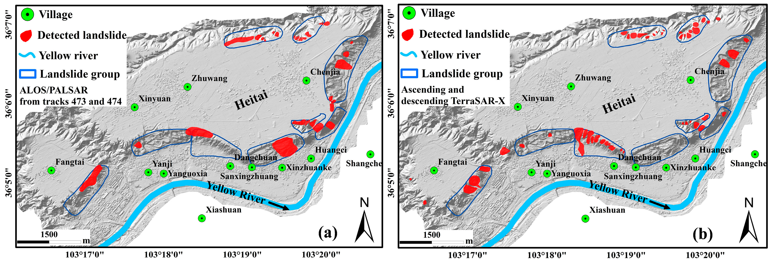
- It can be seen from Table 3 that the area of active landslides identified by ALOS/PALSAR datasets from track 473 and track 474 are highly different in the Huangci, Jiaojia and Chenjia landslide groups. The area of active landslides identified on track 474 images is larger than that identified on track 473 images. This difference may be due to the different acquisition times of the two datasets. According to Peng et al. [11] the largest number of landslides occurred in 2007 and 2008, and the acquisition time of track 474 images is mainly concentrated in this period.
4.3. Landslide Identification Based on SAR Intensity Changes and DEM Errors
5. Discussion
5.1. The Effects of Different SAR Sensors and Bands
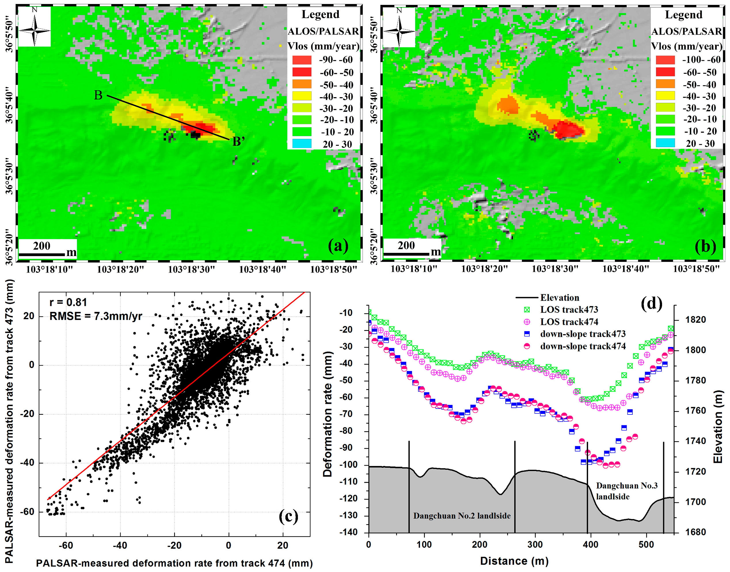
5.2. The Effects of Satellite Track Direction
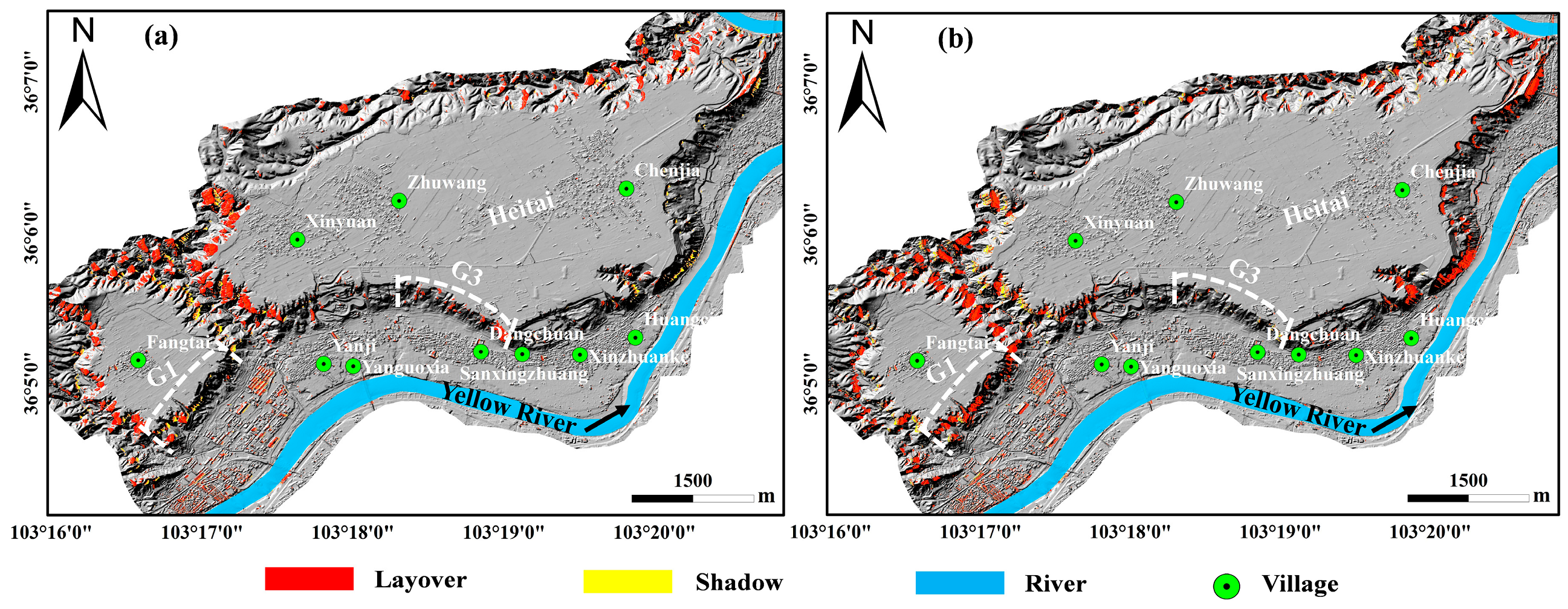
5.3. The Effects of the SAR Geometric Distortions
5.4. The Effects of Differences in Local Incidence Angle between Two Adjacent SAR Satellite Tracks
6. Conclusions
Author Contributions
Funding
Acknowledgments
Conflicts of Interest
References
- Cui, S.H.; Pei, X.J.; Wu, H.Y.; Huang, R.Q. Centrifuge model test of an irrigation-induced loess landslide in the Heifangtai loess platform, Northwest China. J. Mt. Sci. 2018, 15, 130–143. [Google Scholar] [CrossRef]
- Zhao, C.Y.; Zhang, Q.; He, Y.; Peng, J.B.; Yang, C.S.; Kang, Y. Small-scale loess landslide monitoring with small baseline subsets interferometric synthetic aperture radar technique—Case study of Xingyuan landslide, Shaanxi, China. J. Appl. Remote Sens. 2016, 10, 1–14. [Google Scholar] [CrossRef]
- Zhang, D.; Wang, G.; Luo, C.; Chen, J.; Zhou, Y. A rapid loess flowslide triggered by irrigation in China. Landslides 2009, 6, 55–60. [Google Scholar] [CrossRef]
- Zhang, M.S.; Liu, J. Controlling factors of loess landslides in western China. Environ. Earth Sci. 2010, 59, 1671–1680. [Google Scholar] [CrossRef]
- Zhuang, J.Q.; Peng, J.B.; Wang, G.H.; Javed, I.; Wang, Y.; Li, W. Distribution and characteristics of landslide in loess plateau: A case study in Shaanxi province. Eng. Geol. 2018, 36, 89–96. [Google Scholar] [CrossRef]
- Peng, J.B.; Qi, S.W.; Williams, A.; Dijkstra, T.A. Preface to the special issue on “Loess engineering properties and loess geohazards”. Eng. Geol. 2018, 236, 1–3. [Google Scholar] [CrossRef]
- Xu, L.; Dai, F.C.; Kang, G.L.; Tham, L.G.; Tu, X.B. Analysis of some special engineering-geological problems of loess landslide. Chin. J. Geotech. Eng. 2009, 31, 288–292. (In Chinese) [Google Scholar]
- Wang, J.J.; Liang, Y.; Zhang, H.P.; Wu, Y.; Lin, X. A loess landslide induced by excavation and rainfall. Landslides 2014, 11, 141–152. [Google Scholar] [CrossRef]
- Xu, L.; Dai, F.C.; Gong, Q.M.; Tham, L.G.; Min, H. Irrigation-induced loess flow failure in Heifangtai Platform, North-West China. Environ. Earth Sci. 2012, 66, 1707–1713. [Google Scholar] [CrossRef]
- Guzzetti, F.; Mondini, A.C.; Cardinali, M.; Fiorucci, F.; Santangelo, M.; Chang, K.T. Landslide inventory maps: New tools for an old problem. Earth-Sci. Rev. 2012, 112, 42–66. [Google Scholar] [CrossRef]
- Peng, D.L.; Xu, Q.; Liu, F.Z.; He, Y.S.; Zhang, S.; Qi, X.; Zhao, K.Y.; Zhang, X.L. Distribution and failure modes of the landslides in Heitai terrace, China. Eng. Geol. 2018, 236, 97–110. [Google Scholar] [CrossRef]
- Catani, F.; Farina, P.; Moretti, S.; Nico, G.; Strozzi, T. On the application of SAR interferometry to geomorphological studies: Estimation of landform attributes and mass movements. Geomorphology 2005, 66, 119–131. [Google Scholar] [CrossRef]
- Strozzi, T.; Farina, P.; Corsini, A.; Ambrosi, C.; Thuring, M.; Zilger, J.; Wiesmann, A.; Wegmüller, U.; Werner, C. Survey and monitoring of landslide displacements by means of L-band satellite SAR interferometry. Landslides 2005, 2, 193–201. [Google Scholar] [CrossRef]
- Liao, M.S.; Tang, J.; Wang, T.; Balz, T.; Zhang, L. Landslide monitoring with high-resolution SAR data in the Three Gorges region. Sci. China Earth Sci. 2012, 4, 590–601. [Google Scholar] [CrossRef]
- Ferretti, A.; Prati, C.; Rocca, F. Permanent scatterers in SAR interferometry. IEEE Trans. Geosci. Remote Sens. 2001, 39, 8–20. [Google Scholar] [CrossRef] [Green Version]
- Werner, C.; Wegmuller, U.; Strozzi, T.; Wiesmaenn, A. Interferometric point target analysis for deformation mapping. In Proceedings of the IEEE Geoscience and Remote Sensing Symposium (IGARSS), Toulouse, France, 21–25 July 2003; pp. 4362–4364. [Google Scholar]
- Duro, J.; Inglada, J.; Closa, J.; Adam, N.; Arnaud, A. High resolution differential interferometry using time series of ERS and ENVISAT SAR data. In Proceedings of the Fringe 2003 Workshop, Frascati, Italy, 1–5 December 2003. ESA Special Publication, SP-550. [Google Scholar]
- Hooper, A.; Zebker, H.; Segall, P.; Kampes, B. A new method for measuring deformation on volcanoes and other natural terrains using InSAR persistent scatterers. Geophys. Res. Lett. 2004, 31, L23611. [Google Scholar] [CrossRef]
- Bovenga, F.; Refice, A.; Nutricato, R.; Guerriero, L.; Chiaradia, M.T. SPINUA: A flexible processing chain for ERS/ENVISAT long term interferometry. In Proceedings of the ESA-ENVISAT Symposium, Salzburg, Austria, 6–10 September 2004. ESA Special Publication, SP-572. [Google Scholar]
- Kampes, B.M. Deformation Parameter Estimation Using Permanent Scatterer Interferometry. Ph.D. Thesis, Delft University of Technology, Delft, The Netherlands, 2005. [Google Scholar]
- Van der Kooij, M.; Hughes, W.; Sato, S.; Poncos, V. Coherent target monitoring at high spatial density, examples of validation results. In Proceedings of the Fringe 2005 Workshop, Frascati, Italy, 28 November–2 December 2005. ESA Special Publication, SP-610. [Google Scholar]
- Crosetto, M.; Biescas, E.; Duro, J. Generation of advanced ERS and Envisat interferometric SAR products using the stable point network technique. Photogramm. Eng. Remote Sens. 2008, 4, 443–450. [Google Scholar] [CrossRef]
- Berardino, P.; Fornaro, G.; Lanari, R.; Sansosti, E. A new algorithm for surface deformation monitoring based on small baseline differential SAR interferograms. IEEE Trans. Geosci. Remote Sens. 2002, 40, 2375–2383. [Google Scholar] [CrossRef]
- Doin, M.P.; Guillaso, S.; Jolivet, R.; Lasserre, C.; Lodge, F.; Ducret, G. Presentation of the small baseline NSBAS processing chain on a case example: The Etna deformation monitoring from 2003 to 2010 using Envisat data. In Proceedings of the ESA FRINGE 2011 Conference, Frascati, Italy, 19–23 September 2011; pp. 19–23. [Google Scholar]
- Hetland, E.A.; Muse, P.; Simons, M.; Lin, Y.N.; Agram, P.S.; Di Caprio, C.J. Multiscale InSAR time series (MInTS) analysis of surface deformation. J. Geophys. Res. 2012, 117, B02404. [Google Scholar] [CrossRef]
- Samsonov, S.; D’Oreye, N.; Smets, B. Ground deformation associated with post-mining activity at the French–German border revealed by novel InSAR time series method. Int. J. Appl. Earth Obs. Geoinf. 2013, 23, 142–154. [Google Scholar] [CrossRef]
- Zhao, C.Y.; Lu, Z.; Zhang, Q.; Fuente, J.D.L. Large-area landslide detection and monitoring with ALOS/PALSAR imagery data over Northern California and Southern Oregon, USA. Remote Sens. Environ. 2012, 124, 348–359. [Google Scholar] [CrossRef]
- Calò, F.; Ardizzone, F.; Castaldo, R.; Lollino, P.; Tizzani, P.; Guzzetti, F.; Lanari, R.; Angeli, M.G.; Pontoni, F.; Manunta, M. Enhanced landslide investigations through advanced DInSAR techniques: The Ivancich case study, Assisi, Italy. Remote Sens. Environ. 2014, 142, 69–82. [Google Scholar] [CrossRef]
- Sun, Q.; Zhang, L.; Ding, X.L.; Hu, J.; Li, Z.W.; Zhu, J.J. Slope deformation prior to Zhouqu, China landslide from Insar time series analysis. Remote Sens. Environ. 2015, 156, 45–57. [Google Scholar] [CrossRef]
- Kang, Y.; Zhao, C.Y.; Zhang, Q.; Lu, Z.; Li, B. Application of InSAR techniques to an analysis of the Guanling landslide. Remote Sens. 2017, 9, 1046. [Google Scholar] [CrossRef]
- Rosi, A.; Tofani, V.; Tanteri, L.; Stefanelli, C.T.; Agostini, A.; Catani, F.; Casagli, N. The new landslide inventory of Tuscany (Italy) updated with PS-InSAR: Geomorphological features and landslide distribution. Landslide 2017, 1, 1–15. [Google Scholar] [CrossRef]
- Intrieri, E.; Raspini, F.; Fumagalli, A.; Lu, P.; Del Conte, S.; Farina, P.; Allievi, J.; Ferretti, A.; Casagli, N. The Maoxian landslide as seen from space: Detecting and precursors of failure with Sentinel-1 data. Landslides 2017, 15, 123–133. [Google Scholar] [CrossRef]
- Bayer, B.; Simoni, A.; Schmidt, D.; Bertello, L. Using advanced InSAR techniques to monitoring landslide deformations induced by tunneling in the Northern Apennines, Italy. Eng. Geol. 2017, 226, 20–32. [Google Scholar] [CrossRef]
- Schlögel, R.; Thiesbes, B.; Mulas, M.; Guozzo, G.; Notarnicola, C.; Schneiderbauer, S.; Crespi, M.; Mazzoni, A.; Mair, V.; Corsini, A. Multi-temporal X-band radar interferometry using corner Reflectors: Application and validation at the Corvara landslide (Dolomites, Italy). Remote Sens. 2017, 9, 739. [Google Scholar] [CrossRef]
- Bayer, B.; Simoni, A.; Mulas, M.; Corsini, A.; Schmidt, D. Deformation responses of slow moving landslides to seasonal rainfall in the Northern Apennines, measured by InSAR. Geomorphology 2018, 308, 293–306. [Google Scholar] [CrossRef]
- Raspini, F.; Bianchini, S.; Ciampalini, A.; Del Soldato, M.; Solari, L.; Novali, F.; Del Conte, S.; Rucci, A.; Ferretti, A.; Casagli, N. Continuous, semi-automatic monitoring of ground deformation using Sentinel-1 satellites. Sci. Rep. 2018, 8, 7253. [Google Scholar] [CrossRef] [PubMed]
- Zhang, Y.; Meng, X.M.; Jordan, C.; Novellino, A.; Dijkstra, T.; Chen, G. Investigating slow-moving landslides in the Zhouqu region of China using InSAR time series. Landslides 2018, 5, 1–17. [Google Scholar] [CrossRef]
- Del Soldato, M.; Riquelme, A.; Bianchini, S.; Tomàs, R.; Di Martire, D.; De Vita, P.; Moretti, S.; Calcaterra, D. Multisource data integration to investigate one century of evolution for the Agnone landslide (Molise, southern Italy). Landslide 2018, 1–16. [Google Scholar] [CrossRef]
- Frattini, P.; Crosta, G.B.; Rossini, M.; Allievi, J. Activity and Kinematic behavior of deep-seated landslides from PS-InSAR displacement rate measurements. Landslides 2018, 1–2, 1–18. [Google Scholar]
- Hosseini, F.; Pichierri, M.; Eppler, J.; Rabus, B. Starting Spotlight TerraSAR-X SAR interferometry for identification and monitoring of small-scale landslide deformation. Remote Sens. 2018, 10, 844. [Google Scholar] [CrossRef]
- Bordoni, M.; Boni, R.; Colombo, A.; Lanteri, L.; Meisina, C. A methodology for ground motion area detection (GMA-D) using A-DInSAR time series in landslide investigations. Catena 2018, 163, 89–110. [Google Scholar] [CrossRef]
- Dong, J.; Liao, M.S.; Xu, Q.; Zhang, L.; Tang, M.G.; Gong, J.Y. Detection and displacement characterization of landslides using multi-temporal satellites SAR interferometry: A case study of Danba County in the Dadu River Basin. Eng. Geol. 2018, 240, 95–109. [Google Scholar] [CrossRef]
- Zhao, C.Y.; Kang, Y.; Zhang, Q.; Lu, Z.; Li, B. Landslide identification and monitoring along the Jinsha river catchment (Wudongde reservoir area), China, using the InSAR method. Remote Sens. 2018, 10, 993. [Google Scholar] [CrossRef]
- Duan, Z. Study on the Trigger Mechanism of Loess Landslide—A Case of the Loess Landslide in the South Bank of Lower Jing River. Ph.D. Thesis, Chang’an University, Xi’an, China, 2013. (In Chinese). [Google Scholar]
- Herrera, G.; Gutiérrez, F.; García-Davalillo, J.C.; Guerrero, J.; Notti, D.; Galve, J.P.; Fernández-Merodo, J.A.; Cooksley, G. Multi-sensor advanced dinsar monitoring of very slow landslides: The tena valley case study (central spanish pyrenees). Remote Sens. Environ. 2013, 128, 31–43. [Google Scholar] [CrossRef]
- Mulas, M.; Petitta, M.; Corsini, A.; Schneiderbauer, S.; Mair, F.V.; Iasio, C. Long-term monitoring of a deep-seated slow-moving landslide by mean of C-band and X-band advanced interferometric products: The Corvara in Badia case study (Dolomites, Italy). In Proceedings of the 36th international Symposium on Remote Sensing of Environment, Berlin, Germany, 11–15 May 2015. [Google Scholar]
- Sun, Q.; Hu, J.; Zhang, L.; Ding, X.L. Towards slow-moving landslide monitoring by integrating multi-sensor InSAR time series datasets: The Zhouqu case study, China. Remote Sens. 2016, 8, 908. [Google Scholar] [CrossRef]
- Xu, L.; Dai, F.C.; Tu, X.B.; Tham, L.G.; Zhou, Y.F.; Iqbal, J. Landslide in a loess platform, North-West China. Landslide 2014, 11, 993–1005. [Google Scholar] [CrossRef]
- Qi, X.; Xu, Q.; Liu, F.Z. Analysis of retrogressive loess flowslides in Heifangtai, China. Eng. Geol. 2018, 236, 119–128. [Google Scholar] [CrossRef]
- Pan, P.; Shang, Y.Q.; Lü, Q.; Yu, Y. Periodic recurrence and scale-expansion mechanism of loess landslides caused by groundwater seepage and erosion. Bull. Eng. Geol. Environ. 2017, 6, 1–13. [Google Scholar] [CrossRef]
- Xu, Q.; Li, H.J.; He, Y.S.; Liu, F.Z.; Peng, D.L. Comparison of data-driven models of loess landslide runout distance estimation. Bull. Eng. Geol. Environ. 2017, 8, 1–14. [Google Scholar] [CrossRef]
- Xu, L.; Dai, F.C.; Tham, L.G.; Tu, X.B.; Min, H.; Zhou, Y.F.; Wu, C.X.; Xu, K. Field testing of irrigation effects on the stability of a cliff edge in loess, North-west China. Eng. Geol. 2011, 120, 10–17. [Google Scholar] [CrossRef]
- Zhou, Y.F.; Tham, L.G.; Yan, R.W.M.; Xu, L. The mechanism of soil failures along cracks subjected to water infiltration. Comput. Geotech. 2014, 55, 330–341. [Google Scholar] [CrossRef]
- Zeng, R.Q.; Meng, X.M.; Zhang, F.Y.; Wang, S.Y.; Cui, Z.J.; Zhang, M.S.; Zhang, Y.; Chen, G. Characterizing hydrological processes on loess slopes using electrical resistivity tomography—A case study of the Heifangtai terrace, Northwest China. J. Hydrol. 2016, 541, 742–753. [Google Scholar] [CrossRef]
- Zhang, F.Y.; Wang, G.H. Effect of irrigation-induced densification on the post-failure behavior of loess flowslides occurring on the Heifangtai area, Gansu, China. Eng. Geol. 2018, 236, 111–118. [Google Scholar] [CrossRef]
- Peng, J.B.; Zhang, F.Y.; Wang, G.H. Rapid loess flow slides in Heifangtai terrace, Gansu, China. Q. J. Eng. Geol. Hydrogeol. 2017, 50, 106–110. [Google Scholar] [CrossRef]
- The State Key Laboratory of Geohazard Prevention and Geoenvironment Protection has Again Successfully Warned Heifangtai Loess Landslide of Gansu Province. Available online: http://www.cdut.edu.cn/xww/news/150751561027123254.html (accessed on 21 September 2018).
- Lu, Z.; Dzurisin, D.; Jung, H.S.; Zhang, J.; Zhang, Y. Radar image and data fusion for natural hazards characterization. Int. J. Image Data Fusion. 2010, 1, 217–242. [Google Scholar] [CrossRef]
- Hooper, A.; Segall, P.; Zebker, H. Persistent scatterer InSAR for crustal deformation analysis, with application to Volcan Aldedo Galapagos. J. Geophys. Res. 2007, 112, B07407. [Google Scholar] [CrossRef]
- Goldstein, R.; Werner, C. Radar interferogram filtering for geophysical applications. Geophys. Res. Lett. 1998, 21, 4035–4038. [Google Scholar] [CrossRef]
- Costantini, M. A novel phase unwrapping method based on network programming. IEEE Trans. Geosci. Remote Sens. 1998, 36, 813–821. [Google Scholar] [CrossRef]
- Lyons, S.; Sandwell, D. Fault creep along the southern San Andreas from interferometric synthetic aperture radar, permanent scatterers, and stacking. J. Geophys. Res. Solid Earth 2003, 108. [Google Scholar] [CrossRef] [Green Version]
- Bayer, B.; Schmidit, D.; Simoni, A. The influence of external digital elevation models on PS-InSAR and SBAS Results: Implications for the analysis of deformation signals caused by slow moving landslides in the Northern Apennines (Italy). IEEE Trans. Geosci. Remote Sens. 2017, 55, 2618–2631. [Google Scholar] [CrossRef]
- López-Quiroz, P.; Doin, M.P.; Tupin, F.; Briole, P.; Nicolas, J.M. Time series analysis of Mexico City subsidence constrained by radar interferometry. J. Appl. Geophys. 2009, 69, 1–15. [Google Scholar] [CrossRef]
- Yang, Y.; Pepe, A.; Manzo, M.; Casu, F.; Lanari, R. A region-growing technique to improve multi-temporal DInSAR interferogram phase unwrapping performance. Remote Sens. Lett. 2013, 10, 988–997. [Google Scholar] [CrossRef]
- Biggs, J.; Wright, T.; Lu, Z.; Parsons, B. Multi-interferogram method for measuring interseismic deformation: Denali, Fault, Alaska. Geophys. J. Int. 2007, 170, 1165–1179. [Google Scholar] [CrossRef]
- Peng, D.L.; Xu, Q.; Dong, X.J.; Ju, Y.Z.; Qi, X.; Tao, Y.Q. Application of unmanned aerial vehicles low altitude photogrammetry in investigation and evaluation of loess landslide. Adv. Earth Sci. 2017, 32, 319–330. (In Chinese) [Google Scholar]
- Zhang, Q.; Zhao, C.Y. Semiautomatic object-oriented loess landslide recognition based on high-resolution remote sensing images in Heifangtai, Gansu. J. Catastrophol. 2017, 32, 210–215. (In Chinese) [Google Scholar]
- Ju, X.Z. Early Recognition of Loess Landslide Based on UAV Photogrammetry- A Case Study of Heifangtai Terrace. Master’s Thesis, Chengdu University of Technology, Chengdu, China, 2017. (In Chinese). [Google Scholar]


| Satellite | Band | Track | Geometry | Incidence Angle (°) | Resolution in Azimuth (m) and Range (m) | Number of SAR Images |
|---|---|---|---|---|---|---|
| ALOS/PALSAR | L | 473 | Ascending | 38.7385 | 3.16 × 4.7 | 22 |
| ALOS/PALSAR | L | 474 | Ascending | 38.7263 | 3.14 × 4.7 | 12 |
| ALOS/PALSAR-2 | L | 146 | Ascending | 40.5539 | 3.25 × 4.29 | 6 |
| ALOS/PALSAR-2 | L | 39 | Descending | 40.5551 | 3.25 × 4.29 | 5 |
| TerraSAR-X | X | 21 | Ascending | 41.1669 | 1.26 × 0.91 | 23 |
| TerraSAR-X | X | 165 | Descending | 41.8010 | 1.26 × 0.91 | 19 |
| Sentinel-1A/B | C | 135 | Descending | 33.7927 | 9.32 × 13.97 | 24 |
| Datasets | Track | Multilooking Factor | Temporal Threshold (day) | Baseline Threshold (m) | Interferograms Used |
|---|---|---|---|---|---|
| ALOS/PALSAR | 473 | 1 × 2 | 500 | 2000 | 38 |
| ALOS/PALSAR | 474 | 1 × 2 | 500 | 2000 | 19 |
| ALOS/PALSAR-2 | 146 | 1 × 2 | 600 | 500 | 8 |
| ALOS/PALSAR-2 | 39 | 1 × 2 | 600 | 500 | 7 |
| TerraSAR-X | 21 | 2 × 2 | 60 | 250 | 30 |
| TerraSAR-X | 165 | 2 × 2 | 60 | 250 | 25 |
| Sentinel-1A/B | 135 | 4 × 1 | 48 | 200 | 44 |
| Landslide Group | Detected SAR Data | Track | Period | Area (km2) |
|---|---|---|---|---|
| Fangtai | ALOS/PALSAR | 473 | December 2006–March 2011 | 0.0795 |
| ALOS/PALSAR | 474 | March 2007–October 2009 | 0.0708 | |
| ALOS/PALSAR-2 | 146 | November 2014–November 2017 | 0.0678 | |
| ALOS/PALSAR-2 | 39 | May 2015–July 2017 | 0.0042 | |
| TerraSAR-X | 21 | February 2016–November 2016 | 0.0582 | |
| TerraSAR-X | 165 | January 2016–November 2016 | 0.0076 | |
| Xinyuan | ALOS/PALSAR | 473 | December 2006–March 2011 | 0.0059 |
| ALOS/PALSAR | 474 | March 2007–October 2009 | 0.0069 | |
| ALOS/PALSAR-2 | 146 | November 2014–November 2017 | 0.0064 | |
| ALOS/PALSAR-2 | 39 | May 2015–July 2017 | 0.0108 | |
| TerraSAR-X | 21 | February 2016–November 2016 | 0.0075 | |
| TerraSAR-X | 165 | January 2016–November 2016 | 0.0165 | |
| Dangchuan | ALOS/PALSAR | 473 | December 2006–March 2011 | 0.1024 |
| ALOS/PALSAR | 474 | March 2007–October 2009 | 0.0951 | |
| ALOS/PALSAR-2 | 146 | November 2014–November 2017 | 0.1016 | |
| ALOS/PALSAR-2 | 39 | May 2015–July 2017 | 0.1672 | |
| TerraSAR-X | 21 | February 2016–November 2016 | 0.0933 | |
| TerraSAR-X | 165 | January 2016–November 2016 | 0.1391 | |
| Sentinel-1A/B | 135 | September 2016–October 2017 | 0.1610 | |
| Huangci | ALOS/PALSAR | 473 | December 2006–March 2011 | 0.1168 |
| ALOS/PALSAR | 474 | March 2007–October 2009 | 0.1862 | |
| Yehugou | ALOS/PALSAR | 473 | December 2006–March 2011 | 0.0703 |
| ALOS/PALSAR | 474 | March 2007–October 2009 | 0.0634 | |
| ALOS/PALSAR-2 | 146 | November 2014–November 2017 | 0.0313 | |
| ALOS/PALSAR-2 | 39 | May 2015–July 2017 | 0.0184 | |
| TerraSAR-X | 21 | February 2016–November 2016 | 0.0311 | |
| TerraSAR-X | 165 | January 2016–November 2016 | 0.0323 | |
| Sentinel-1A/B | 135 | September 2016–October 2017 | 0.0420 | |
| Jiaojiaya | ALOS/PALSAR | 473 | December 2006–March 2011 | 0.0018 |
| ALOS/PALSAR | 474 | March 2007–October 2009 | 0.0007 | |
| TerraSAR-X | 21 | February 2016–November 2016 | 0.0023 | |
| Jiaojia | ALOS/PALSAR | 473 | December 2006–March 2011 | 0.0425 |
| ALOS/PALSAR | 474 | March 2007–October 2009 | 0.0544 | |
| ALOS/PALSAR-2 | 146 | November 2014–November 2017 | 0.0202 | |
| ALOS/PALSAR-2 | 39 | May 2015–July 2017 | 0.0043 | |
| TerraSAR-X | 21 | February 2016–November 2016 | 0.0309 | |
| TerraSAR-X | 165 | January 2016–November 2016 | 0.0413 | |
| Sentinel-1A/B | 135 | September 2016–October 2017 | 0.0035 | |
| Chenjia | ALOS/PALSAR | 473 | December 2006–March 2011 | 0.0361 |
| ALOS/PALSAR | 474 | March 2007–October 2009 | 0.0622 | |
| ALOS/PALSAR-2 | 146 | November 2014–November 2017 | 0.0130 | |
| ALOS/PALSAR-2 | 39 | May 2015–July 2017 | 0.0275 | |
| TerraSAR-X | 21 | February 2016–November 2016 | 0.0345 | |
| TerraSAR-X | 165 | January 2016–November 2016 | 0.0128 | |
| Sentinel-1A/B | 135 | September 2016–October 2017 | 0.0413 | |
| Moshigou | ALOS/PALSAR | 473 | December 2006–March 2011 | 0.0300 |
| ALOS/PALSAR | 474 | March 2007–October 2009 | 0.0402 | |
| ALOS/PALSAR-2 | 146 | November 2014–November 2017 | 0.0691 | |
| ALOS/PALSAR-2 | 39 | May 2015–July 2017 | 0.0675 | |
| TerraSAR-X | 21 | February 2016–November 2016 | 0.0509 | |
| TerraSAR-X | 165 | January 2016–November 2016 | 0.0569 | |
| Sentinel-1A/B | 135 | September 2016–October 2017 | 0.0814 |
© 2018 by the authors. Licensee MDPI, Basel, Switzerland. This article is an open access article distributed under the terms and conditions of the Creative Commons Attribution (CC BY) license (http://creativecommons.org/licenses/by/4.0/).
Share and Cite
Liu, X.; Zhao, C.; Zhang, Q.; Peng, J.; Zhu, W.; Lu, Z. Multi-Temporal Loess Landslide Inventory Mapping with C-, X- and L-Band SAR Datasets—A Case Study of Heifangtai Loess Landslides, China. Remote Sens. 2018, 10, 1756. https://0-doi-org.brum.beds.ac.uk/10.3390/rs10111756
Liu X, Zhao C, Zhang Q, Peng J, Zhu W, Lu Z. Multi-Temporal Loess Landslide Inventory Mapping with C-, X- and L-Band SAR Datasets—A Case Study of Heifangtai Loess Landslides, China. Remote Sensing. 2018; 10(11):1756. https://0-doi-org.brum.beds.ac.uk/10.3390/rs10111756
Chicago/Turabian StyleLiu, Xiaojie, Chaoying Zhao, Qin Zhang, Jianbing Peng, Wu Zhu, and Zhong Lu. 2018. "Multi-Temporal Loess Landslide Inventory Mapping with C-, X- and L-Band SAR Datasets—A Case Study of Heifangtai Loess Landslides, China" Remote Sensing 10, no. 11: 1756. https://0-doi-org.brum.beds.ac.uk/10.3390/rs10111756