Article

Quantification of Extent, Density, and Status of Aquatic Reed Beds Using Point Clouds Derived from UAV–RGB Imagery

Aquatic Systems Biology Unit, Limnological Research Station Iffeldorf, Department of Ecology and Ecosystem Management, Technical University of Munich, Hofmark 1-3, 82393 Iffeldorf, Germany
*
Author to whom correspondence should be addressed.
Remote Sens. 2018, 10(12), 1869; https://0-doi-org.brum.beds.ac.uk/10.3390/rs10121869
Submission received: 11 September 2018 / Revised: 31 October 2018 / Accepted: 21 November 2018 / Published: 23 November 2018
(This article belongs to the Special Issue Drone Remote Sensing)

Abstract

:
Quantification of reed coverage and vegetation status is fundamental for monitoring and developing lake conservation strategies. The applicability of Unmanned Aerial Vehicles (UAV) three-dimensional data (point clouds) for status evaluation was investigated. This study focused on mapping extent, density, and vegetation status of aquatic reed beds. Point clouds were calculated with Structure from Motion (SfM) algorithms in aerial imagery recorded with Rotary Wing (RW) and Fixed Wing (FW) UAV. Extent was quantified by measuring the surface between frontline and shoreline. Density classification was based on point geometry (height and height variance) in point clouds. Spectral information per point was used for calculating a vegetation index and was used as indicator for vegetation vitality. Status was achieved by combining data on density, vitality, and frontline shape outputs. Field observations in areas of interest (AOI) and optical imagery were used for reference and validation purposes. A root mean square error (RMSE) of 1.58 m to 3.62 m for cross sections from field measurements and classification was achieved for extent map. The overall accuracy (OA) acquired for density classification was 88.6% (Kappa = 0.8). The OA for status classification of 83.3% (Kappa = 0.7) was reached by comparison with field measurements complemented by secondary Red, Green, Blue (RGB) data visual assessments. The research shows that complex transitional zones (water–vegetation–land) can be assessed and support the suitability of the applied method providing new strategies for monitoring aquatic reed bed using low-cost UAV imagery.

Graphical Abstract

1. Introduction

Reed beds located in freshwater lakes around shores can be categorized into three ecological zones. Land, transitional, and aquatic reeds have been mapped according to the lake’s water level. Land reed grows in rarely flooded areas, has a lower stem density and height compared to the transitional reed, and is a stand mixed with other species (e.g., Thypa, Scripus, Carex). Transitional reed is flooded periodically and has the highest stem density and height. Between aquatic and transitional reed, a significant break in height can often be noticed. Aquatic reed stands in water throughout the year and forms the reed expansion front, representing the boundary to the lakeside. It is the most sensitive area in a reed stock and, under favorable conditions, it is able to develop further rhizomes and spread lakeward. Aquatic reed is characterized by a lower stem density and a lower height. Aquatic reed, as well as transitional reed, are normally pure stands consisting of Phragmites australis [1].
Aquatic reed beds play an important role in lake systems that can be linked to ecosystem services. They stabilize and protect the shores from erosion reducing wave energy, with its dense root system and stems distribution [2]. They support the assimilation of nutrients, which is fundamental for the balance of nitrogen, phosphorus, and silicon [3,4]. Reed beds also function as habitat and nurture supply. Reeds are decomposed by fungi and bacteria and provide nutrients for detritus and grazers, which are eaten by insects, toad bugs, and omnivore water birds. The undisturbed aquatic reed, and the reduced wave energy make it a preferred habitat for reptiles, amphibians, and an ideal location for fish spawn. Regarding cultural ecosystem services, reed beds belong to the dominating elements of a pictorial landscape [1]. Growing at lakes shores, they are associated with near-natural landscape, which is considered as an important aspect for recreation [5].
The decline of aquatic reed beds in central Europe during the last decades has already been documented [6,7,8]. The suggested reasons for the decline include direct destruction by land expansion, recreational traffic, summer mowing, and mechanical destruction by waves, rubbish, or driftwood. Further identified potential reasons for decline are the grazing by waterfowl and other animals (e.g., gray goose, swans, black coot, muskrat, nutria, and grass carp) and domestic animals (e.g., cows and horses), and the degradation of the water and sediment quality caused by eutrophication [7]. Since an increment in the frequency and severity of extreme events, such as floods and drought, is predicted [9,10], changes in water regimes producing very low to extreme high water levels are also suspected to result in the decline of aquatic reed populations.
In order to monitor and develop adequate protection and conservation strategies, quantification of aquatic reed coverage and its status is fundamental. Aquatic reed extent is calculated by measuring the area between the shore and frontline. Allocation of shoreline position can be challenging since it is prone to changes through time due to sediment movement and tidal fluctuations [11]. In order to test the sensors and systems applied in this study, a clear definition of shoreline was needed. Shoreline, in this study, was defined as the point where water surface and land have the same height, and frontline was defined as the limit at which the aquatic reed expansion front finishes lakeward. Different approaches to describe a reed bed condition are available. Data collected in the field, such as stem density (number of stems per m²), the percentage of panicle bearing shoots, or stem height are indicators of vitality [12,13]. The frontline sinuosity can also be used as indicator for assessing status, since it is an indicator of frayed, ripped, or not zoned aquatic reed stands. The collection of plant morphologic and phenotypical traits in the field represents a traditional method for characterizing a reed stock. This type of collected data might deliver precise information but it is time consuming and requires personnel. Additionally, it causes habitat disturbance and it is often not possible to gain access to high and dense stocks [14]. Field observations have been supported by remote sensing methods, in which aquatic reed was conventionally mapped by manual visual interpretation and manual delineation of images recorded from satellite or airplanes [6,14,15]. This is also true for historical monitoring at Lake Chiemsee, in which aquatic reed beds were quantified through the analysis of aerial imagery provided by the state office for surveying “Landesamt für Digitalisierung, Breitband und Vermessung (LDBV)”. Accurate allocation of frontline and density quantification was, however, restricted in these surveys by spatial resolution and variation in spectral information due to different collecting times [16].
The issues with the quantification of aquatic reed beds encountered in the interpretation of optical imagery, has already been bypassed with the assessment of surface elevation data [17]. The extent at which height of sparse aquatic reed beds can match digitally-modeled reed beds has similarly been evaluated [18]. Nevertheless, the accuracy of coverage quantification and the status assessment of aquatic reed stocks using UAV elevation and spectral information is still uncertain. Remote sensing analysis of vegetation has been frequently performed with the interpretation of spectral reflectance recorded by optical systems [13,14,19,20]. Since spectral information is only recorded from electromagnetic energy reflected on upper surface objects, valuable information from lower structures (e.g., under storey or shoreline) in a vegetation stand is not available. Emerging remote sensing technologies, such as Light Detection And Ranging (LiDAR), and Unmanned Aerial Vehicles (UAV), may offer new possibilities in the status monitoring of aquatic reed beds. LiDAR and UAV deliver data for elevation modeling, which supports a better characterization of vegetation structure and also reduces the possibility of habitat disturbance. LiDAR data has been used to accurately quantify and characterize the structure of aquatic reeds [19,21], but the evaluation of amplitude per each laser return for evaluating vegetation vitality is still unknown. Since LiDAR lacks spectral information, an alternative to produce three-dimensional data (point clouds) with spectral information is by using close-range aerial photogrammetry. Technological advances have improved the performance of UAVs, making them capable of flying longer, auto piloted, and carrying heavier loads. A wide range of instruments have already been tested on UAVs such as visible band, near-infrared, or multispectral cameras, as well as thermal cameras and laser scanners [22]. For instance, UAVs equipped with VNIR (visible and near-infrared) and thermal sensors, record data at decimeter or centimeter spatial resolutions for more accurate monitoring and stress characterization, which represents “a capacity unavailable from satellite based systems” [23].
Optical imagery collected with UAV can be photogrammetrically processed for generating elevation information. The development of automated computer vision techniques (e.g., Structure from Motion—SfM) facilitates the remote sensing of structural and spectral characteristics of vegetation with UAVs [24]. It enables a high-resolution and three-dimensional observation of the vegetation canopy structure by matching overlapped images and generating elevation models [25]. Three-dimensional coordinates of an object can be extracted if it is imaged from two different perspectives, without the need of camera positional information [26]. With a series of overlapping images, objects are matched, the geometric accuracy is improved and the probability of occlusions (shadowed or invisible areas in an image) is reduced. The generation of image-based point clouds requires images with a high-spatial resolution and a multi-image overlap [27]. In addition, spectral information, available in optical imagery collected with UAVs, allows for the calculation of vegetation indexes. In agricultural applications, this information has been used to assess vegetation health and nutrient supply, where high resolution has enabled the separation of single plants from the ground [28]. Multispectral sensors, to calculate the normalized different vegetation index (NDVI), have also been used to describe the status of crops and applied thermal spectral sensors to assess the water supply via the crop water stress index (CWSI) [29]. The temporal flexibility of UAVs has been also tested in forestry to create a time series of multispectral imagery with five narrow bands (red, green, blue, red edge, NIR) to detect appearing stress in crowns of Pinus radiate [30] In this way, UAV-based spectral signatures could also contribute in the status characterization of aquatic reed [31]. Vital leafs of reed show a high reflectance in the green and infrared color and a high absorption in the red wavelength [32]. Reduced vitality is accompanied by degradation and shrinking cells resulting in higher red and lower NIR reflectance.
Analysis of UAV point clouds geometry, in combination with the available spectral information, is expected to deliver more accurate status descriptions of vegetation stocks. Crop damage has already been estimated by analyzing the relations between vegetation canopy height and NDVI values [33]. Discrimination of vegetation types can also be achieved with close-range aerial photogrammetry [34]. In terms of mapping products, the present study faced the challenge of developing an approach that is consistent with the official monitoring method in terms of extent, density, and status determination. High-resolution imagery and elevation information derived from close-range aerial imagery may be suitable in assessment of vegetation. UAVs, in combination with computer vision technique, could also contribute in the coverage quantification, categorization of vegetation density, and status assessment of aquatic reed beds. This study assessed the classification of aquatic reed bed using data obtained through close-range aerial digital photogrammetry. The UAV platform and imaging system were chosen from the consumer sector with a focus on affordability for small companies specialized in UAV mapping for environmental applications. The core objectives addressed were to determine the accuracy of 1) the determination of aquatic reed bed frontline and extent, 2) the classification of aquatic reed density, and 3) the status classification of aquatic reed.

2. Materials and Methods
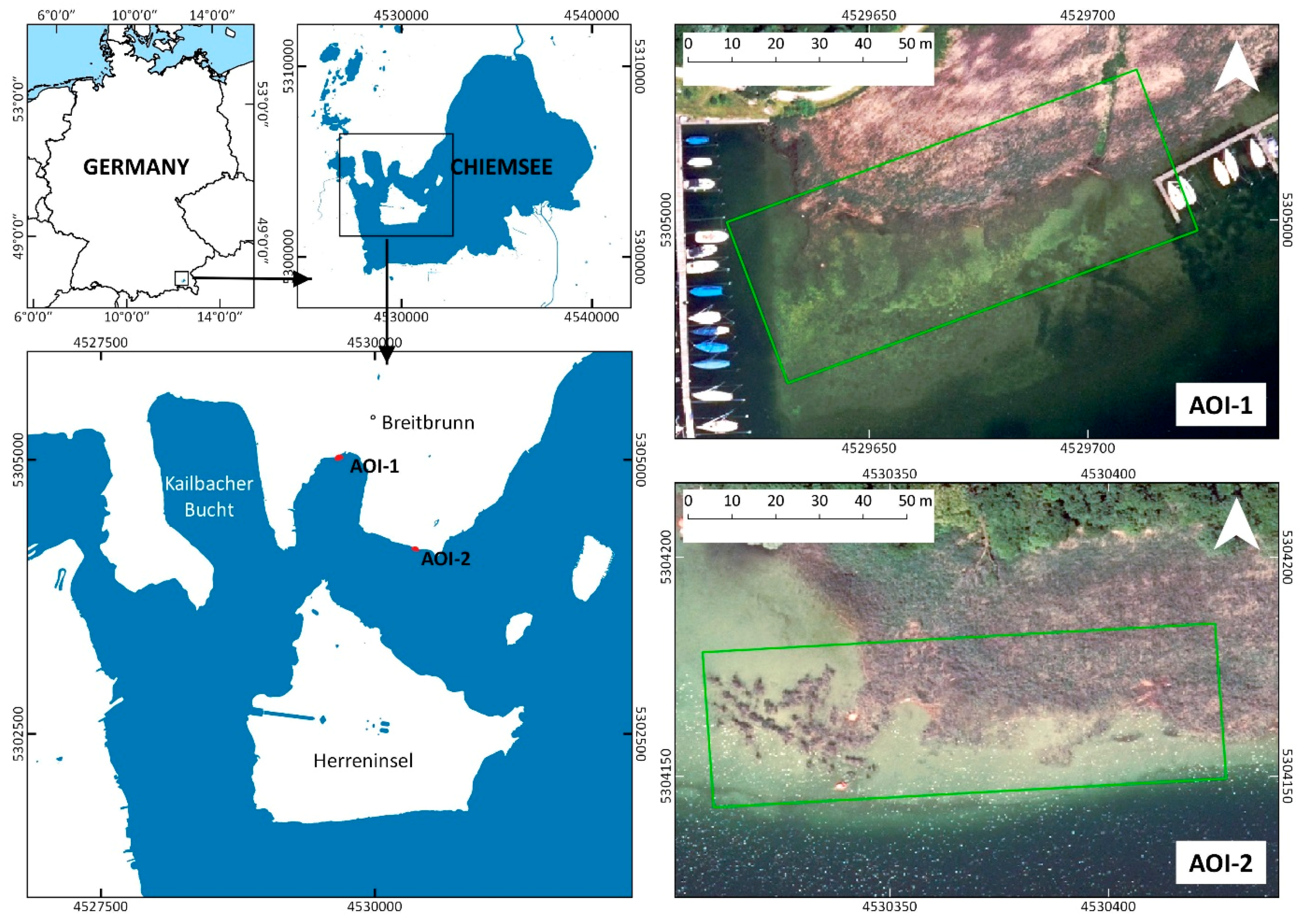
2.1. Study Area

The study area is located approximately 80 km southeast of the city of Munich in Bavaria (Germany). Lake Chiemsee is one of the last intact inland waters in central Europe [16]. Although a significant decline of reed bed has occurred also at the Chiemsee [1], essential aquatic reed populations are still present. The populations of Phragmites australis are not older than approximately 100 years. Visual interpretations of aerial images have revealed that the development of aquatic reed had reached its maximum expansion in 1937. Over the following 20 years, reed population remained stable until the end of 1957, when then start of a decrease was documented. Until 1973, 14% of the reed bed declined in terms of biomass and special extent and reduced further 31% in the following years. In 1982 the reed population slowly stabilized (decreasing 7%) [1]. Further monitoring projects revealed a population increase of 4.5% between 1991 and 1998 [16].

2.2. Description of UAV Point Clouds

Point clouds were photogrammetrically calculated based on aerial imagery collected by UAVs in two different areas of interest (AOI). Surveying missions were deployed on September 21st in 2015 with Rotary-Wing (RW) and Fixed-Wing (FW) UAVs for AOI-1 and AOI-2 (Figure 1), respectively. Growth of reed stands over the year was an important consideration for data recording. At the beginning of the vegetation period, aquatic reed is fast growing, because it needs to emerge for photosynthesis. Therefore, aquatic reed covers 40% of its growth in April. In May, the growth rate is at 20% only, while land reed has a constant growth of 30% between these two months. In June, the aquatic reed’s growth rate rises up to 25%. From then on, it decreases constantly. In October, the growth amounts to only 2%. [1]. Late September was ideal for mapping this kind of vegetation since it has reached its maximum height. Selected AOIs differentiate regarding the structure and represent different characteristics of aquatic reed bed types. AOI-1 and AOI-2 are located at the northwest shore at the border of the community Breitbrunn. From the water to the landside, AOI-1 is characterized by a gradual increase in stem height. Expansion front is frayed causing small vegetation inlets. In AOI-2 reeds grow in groups with increasing height.
Point clouds were generated through the implementation of SfM algorithms in Agisoft Photoscan Professional—Version 1.2.6 [35]. Since camera configuration was the same for all missions, as an effect of the different flying altitude, the point clouds differed in point density (Table 1). RW imagery (AOI-1) allowed clouds with a point density of 2260 points/m², and 1230 points/m² for the FW imagery (AOI-2). Point clouds were georeferenced with ten Ground Control Points (GCP) in case of AOI-1 and eight GCPs for AOI-2 with a differential GPS (Trimble Geo XT). A total of 258 positions were measured with a mean Dilution of Precision (DOP) of 1.1 (α ± 0.5) for the 18 locations. After differential correction, a horizontal precision of 0.4 m was obtained (standard deviation 0.02 m). This allowed a successful georeferencing of point clouds and orthomosaics, and did not interfere with the study objectives. The coordinate reference system used was DHDN Gauss-Krüger Zone 4. Each single point in clouds has geographic coordinates (x, y, z) and a value for each color channel (Red, Green, Blue). Detailed explanation of UAV platforms and settings for point cloud calculation in Agisoft Photoscan can be found in [18].

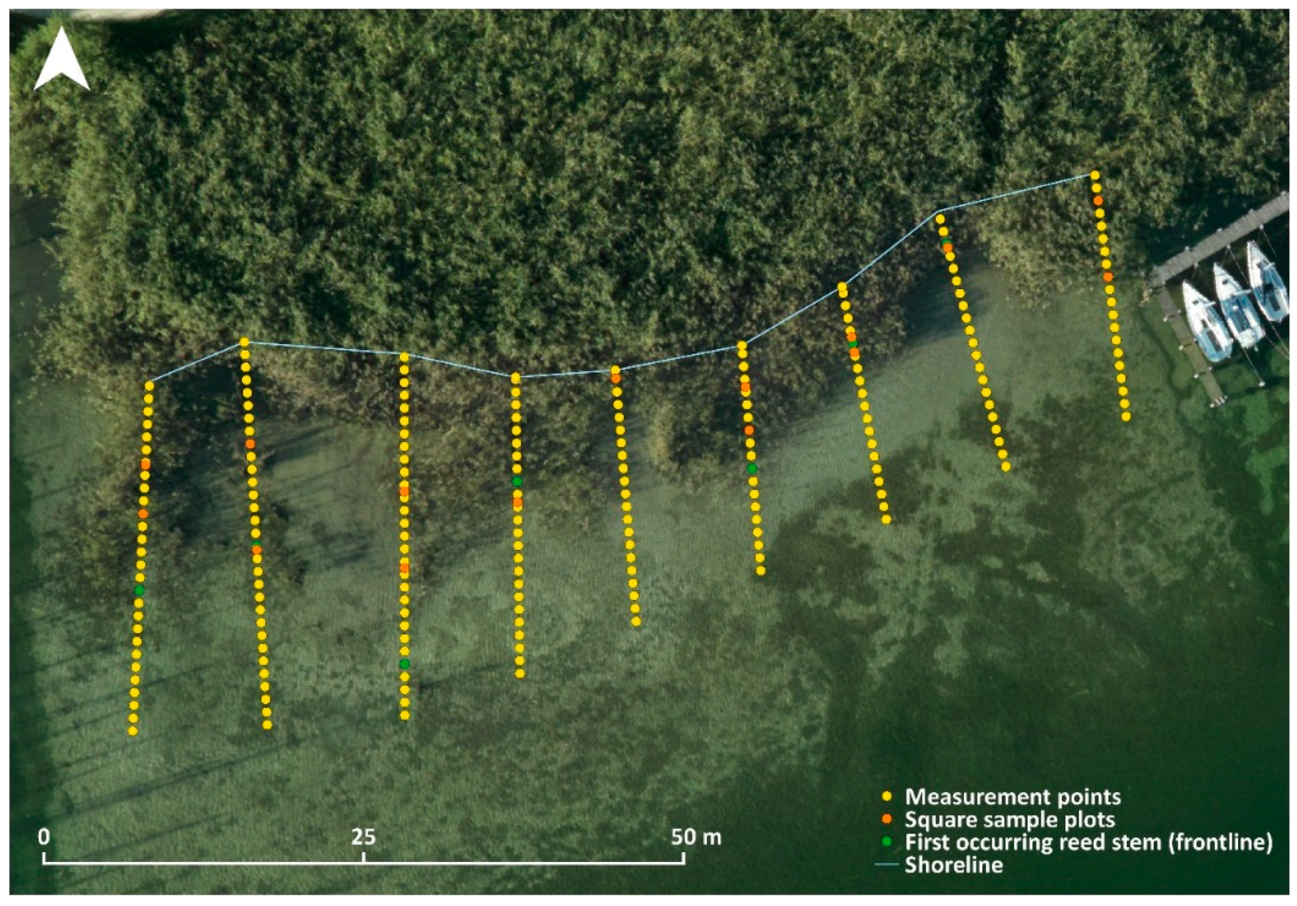
2.3. Reference and Validation Data

Field measurements, orthomosaics from RW and FW UAVs, and aerial imagery were used for reference and validating classifications. Field data were generated through field measurements from September 15th in 2015 based on the protocols [17,18]. They consisted of shoreline perpendicular cross-sections, square sample plots, and shoreline and frontline boundaries. The data available for every cross-section was the stem height and, for square sample plots, the number of stems per square meter, the number of green and dry stems with and without panicles, and the diameter of stems. Square measurements were taken along each cross section in sparse and in dense reed beds (Figure 2). Since measurements took place from water to land side, the frontline corresponds to the first occurring reed stem. The water level on the day of the field measurements was at 517.96 m.a.s.l. [36].
Orthomosaics were created from RW and FW UAVs datasets after running SfM algorithms with Agisoft Photoscan Professional—Version 1.2.6 [35]. Using the same sensor (Canon EOS-M) with 22 mm optics, the spatial resolution was controlled by flying height. AOI-1 achieved a Ground Sampling Distance (GSD) of 2.1 cm/pix and 2.86 cm/pix for AOI-2. In the same way, orthoimagery was referenced in DHDN Gauss-Krüger Zone 4. Additionally, a set of aerial imagery (10 cm GSD) was recorded on the same day of UAV surveys (21st of September 2015) but by a different sensor (Hasselblad H3DII-39 camera, 39 MP) mounted on an aircraft (Airborne Hydro Mapping—AHM) and used as additional verification source.

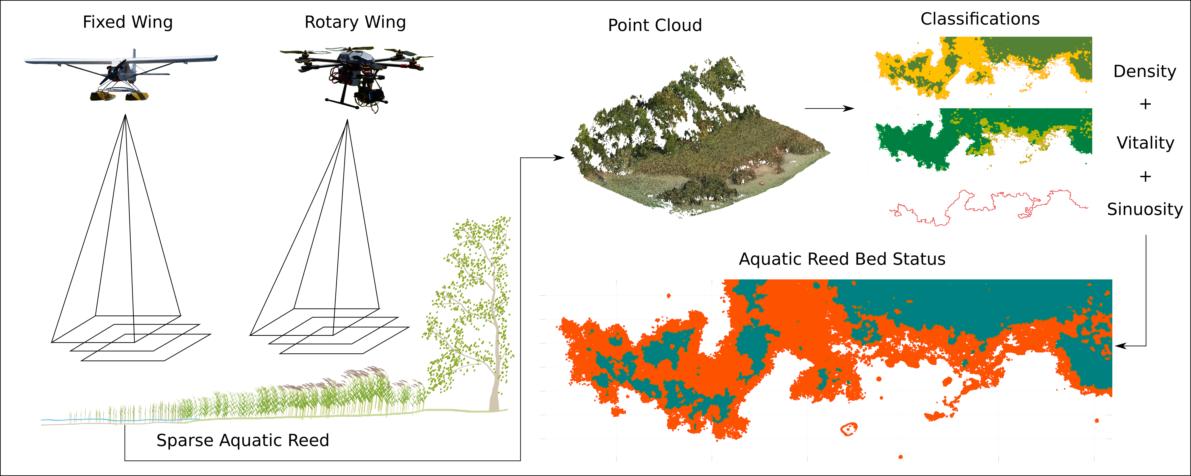
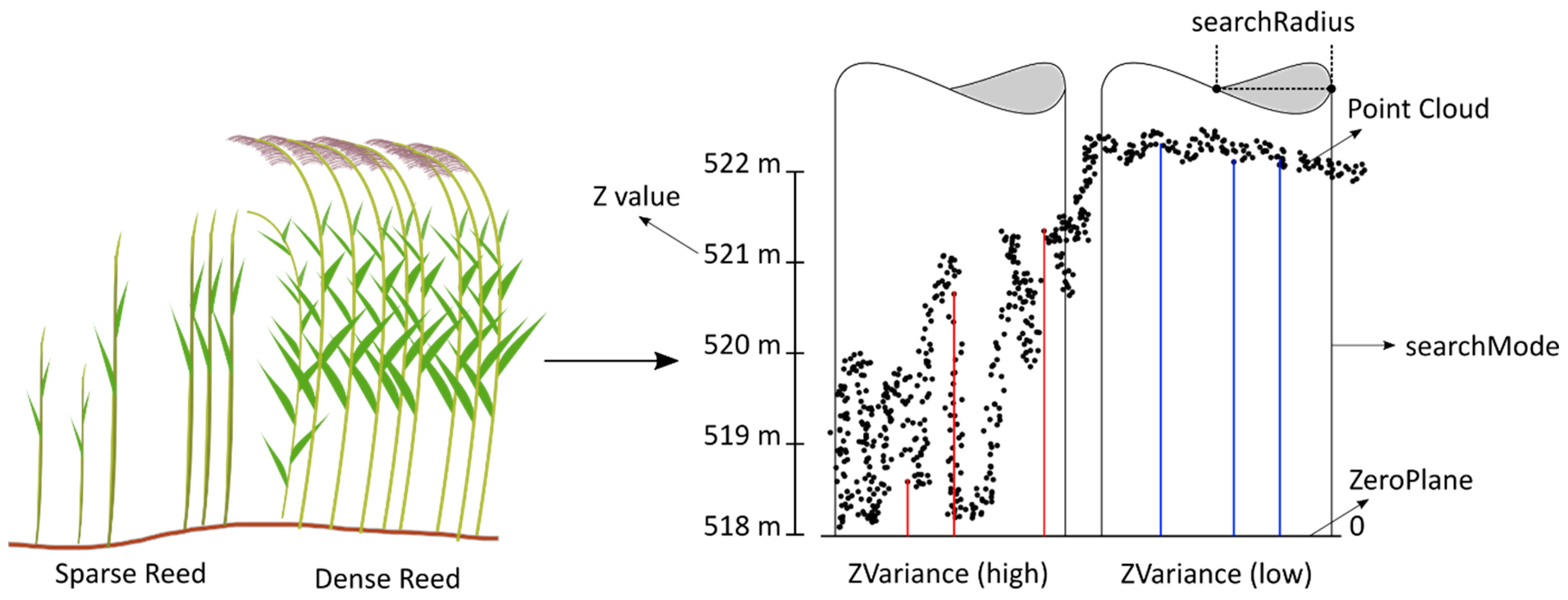
2.4. Classification of Reed Extent and Density in UAV Point Clouds

The software OPALS 2.2.0 (Orientation and Processing of Airborne Laser Scanning data), developed by the Vienna University of Technology, was used for the analysis of the point clouds. OPALS is software based on modules (processing tools), which use information about points stored as attributes [37]. The developed classification script was applied for both AOIs and based on a decision tree. The classification of aquatic reed beds for extent quantification was implemented considering the differences in point heights (z value of a point). The first step was the classification of points in the classes “Water” and “No Water”. The height of water surface provided by the water management office was used as reference to discriminate points corresponding to water/lake-bottom and aquatic reed. Once points corresponding to land and water were identified, categorization of “aquatic reed” points was achieved.
Consistent with the instructions of the last official reed survey at the Chiemsee, the density classes for this study were also assigned to “Dense” and “Sparse” aquatic reed beds [16]. The visual examination of cross-sections along AOIs revealed that density classification can be obtained based on the geometric distribution of points in height (Z axis), and this is how the threshold value for density classification based on decision trees was obtained. Within the class “aquatic reed”, absolute height and variation of points in height are suitable attributes for threshold definition and then classification (Figure 3). These attributes were calculated with the module PointStats. It calculates statistics by selecting a group of points within a specific volume (searchMode) and measuring them from a specific reference point (refModel). Since the analysis was based on distribution of points in the Z axis, a cylinder was used for point selection. Its radius (searchRadius) was defined to 0.5 m with the purpose of being consistent and matching the measurements on field (stems/m²). A plane passing through the origin (zeroPlane) was employed as reference for point measurements. The statistics used for classification were the mean height (Zmean) and the variance of point height (ZVariance).
The statistic Zmean is calculated considering all the points within the cylinder with reference to the zeroPlane. The advantage of using the mean height instead of the absolute height is that differences are avoided resulting in heights that are more homogeneous across the cloud. The statistic ZVariance gives a value of height variations for a group of points with reference to the zeroPlane. The smaller the variation, the more points have the same height. Contrarily to dense stocks, additional features are imaged in areas of sparse aquatic reed beds. Points of leaves, stems, or ground can be found in the cloud, which increases the height variation value (Figure 3). Furthermore, the variance shows abrupt changes in the reed bed, such as ripped areas of the reed front. ZVariance was calculated with the same settings as the Zmean. The closer is the value to 0, the lower the variance and consequently the higher the stand density.

2.5. Estimation of Vegetation Status

The status of the aquatic reed was calculated on the basis of a color index and frontline sinuosity. Band intensity based indices are less sensitive to brightness fluctuations and are therefore more useful than applying only a single color channel [38]. Woebbecke’s excess green (ExG) [39] minus the excess red (ExR) [40] was found to be most effective in separating these classes as well as reed from the ground of the lake, because the index illustrates clear differences in its values. Other studies [38,41] have also tested the ExG–ExR as a useful vegetation index. ExG–ExR index is calculated as:
E x G = 2 g r b ,   E x R = 1.4 r g
where r, g, and b were the chromatic coordinates
r = R R + G + B ,   g = G R + G + B ,   b = B R + G + B
And, R*, G* and B* were the normalized RGB values (0–1) defined
R = R R m ,   G = G G m ,   B = B B m
R, G, and B are the actual values for each color channel of one point. The Rm, Gm, and Bm are the maximum tonal values of each color [38]. The maximum values per channel in the UAV point cloud were 65,280, which approximately correspond to a 16-bit color depth. That information was obtained by using the module OpalsInfo. The mean value was calculated for the ExG–ExR with the using same searchMode, searchRadius, and refModel used for the mean height or the height variance (Figure 4). Based on trial and error and using samples of ExG–ExR values in vital and less vital aquatics reeds was needed to determine the threshold suitable for classification of AOIs simultaneously.
The frontline sinuosity is another element to analyze whether aquatic reed beds are facing stressing factors. The frontline sinuosity is the ratio of the length along the frontline (curvilinear length) and the straight distance between two points (Euclidean distance). Frayed, ripped, or not zoned aquatic reed beds can be allocated by measuring the frontline sinuosity. Frontline sinuosity is calculated as:
F r o n t l i n e   S i n u o s i t y = F r o n t l i n e   l e n g t h   [ m ] F r o n t l i n e   E u c l i d e a n   d i s t a n c e   [ m ]
If the sinuosity index of a reach is 1.3 or greater, the reach is considered as meandering, a straight reach has a sinuosity index of 1 and reaches which is having sinuosity indices between 1.05 and 1.3 are defined as sinuous [42]. Sinuosity index was calculated every 10 meters sections (Total of 18) and the mean value was used for determined if the frontline in the AOIs is low or high sinuous.
Based on the spectral reflectance of reed bed components obtained with ExG–ExR index, areas with a majority of reeds with green leaves and stems (Vital) were discriminated from dried/dying reeds (less vital). Finally, density and vitality classifications were then combined with frontline sinuosity ratio to derive the status. The classes “stressed” and “unstressed” were employed for the status classification. The lower the density and vitality, the more stressed a stand is. Contrarily, unstressed stocks consist of a dense and green vegetation coverage.

2.6. Validation of Classification Results

2.6.1. Reed Bed Extent Quantification and Frontline Assessment

The extent of aquatic reed beds was obtained by measuring the area between shoreline and frontline. Since photogrammetric methods and optical imagery of the allocation of shoreline is not possible, the shoreline measured on site was used to calculate the coverage. Regarding the frontline, length differences between cross sections measured on field and on modeled data was assessed using the Root Mean Square Error (RMSE). In addition, accuracy was also assessed using the DGPS points defined as frontline. Nine and eleven positions were surveyed on every cross-section for AOI-1, and -2 respectively. Thus, 20 frontline locations were checked for conformity.

2.6.2. Accuracy Assessment of Density and Vegetation Status Classification

Accuracy of aquatic reed bed density and vegetation status was assessed by means of an error matrix. It is an effective method since every single class is evaluated individually. Producer’s Accuracy (PA), User’s Accuracy (UA), and Kappa coefficient are the indicators obtained to evaluate the match between field and estimated measurements. PA reveals how well samples for this class are assigned. UA indicates the probability that a classified sample represents the assigned class in real [43]. Kappa coefficient is an indicator to which percentage correct values of an error matrix are “true” agreement (value 1) versus “chance” agreement (value 0) [44]. A third class which represents water, was added to fill empty areas. Thereby, the differentiation of reed and water was also evaluated.
Data collected from 33 squared sample plots and 682 randomly stratified (classes) sample points were used to assess the density map. The true agreement of each sample point was then verified. Regarding the status map, the same strategy was chosen but instead of square sample plots, 384 observations at 1 m distance along transects were used. Measurements reported without reed above the water surface were assigned as “water”, whilst the remaining observations to either “stressed” or “unstressed” reed. This grouping was implemented in order to be consistent with the classified categories. The allocation of unstressed reed was completed by verifying the status, using the reference image provided by Airborne Hydro Mapping (AHM) Company according to the interpretation key (Table 2).

3. Results

3.1. Point Cloud Classification

Aquatic reed bed extent, density, and status were obtained with the implementation of the developed decision tree (Figure 5). Knowledge from field observations, visual inspections of point clouds, and additional independent aerial imagery were fundamental in the categorization process. Calculation of statistical parameters provided variables for more accurate and unbiased classifications. Considering statistical parameters for every point cloud, several classes were categorized. Aquatic reed was identified by allocating the land–water line with the water surface level for the day of flight. Density of aquatic reed beds was achieved by considering the mean height (ZMean) and height variance (ZVariance). The threshold for the mean height parameter was set to 519.5 m, which is 1.45 m with reference to the water surface level (518.05 m). The classification threshold for variance was defined to 0.1 for points with heights smaller than 1.45 m and variance greater than 0.1 were assigned as “sparse”, whilst points with opposite values as “dense”. ExG–ExR index was calculated to determine areas with dominance of vital stems. The threshold for the classification based on the index was determined to −0.105 and assigned classes were “vital” and “less vital”. The threshold assigned for frontline sinuosity was assigned to 0.5. A reed bed with values smaller than 0.5 were classified as “high sinuosity”. The combination of density results and color index contributed in the achievement of classification or reed status. Status was assigned to the classes “stressed” and “unstressed” aquatic reed.

3.2. Extent Quantification and Frontline Assessment

The extents for AOI-1 and AOI-2 were 656 m² and 986 m², respectively. In both cases the classified areas were smaller than the measured area (760 m² and 1179 m² for AOI-1 and AOI-2, respectively). Frontline sinuosity index for AOI-1 was µ 2.9 ± α 1.8 and µ 3.02 ± α 1.8 for AOI-2. Since sinuosity index for both AOIs greater than 1.3, frontlines were categorized as high sinuous (Figure 6). The RMSEs of cross sections confirmed that the classified extent of AOI-2 had a higher agreement. The RMSE of AOI-1 was 3.62 m and 1.58 m for AOI-2. The evaluation of the classified reed frontlines using the 20 locations (nine and 11 for AOI-1 and -2, respectively) resulted in an overall agreement of 70.0%. For AOI-1, seven out of nine points were correctly identified, which resulted in 77.8% agreement. Seven out of eleven points of the measured extent showed an alignment for AOI-2, resulting in a true agreement of 63.6%.

3.3. Accuracy Assessments of Density and Status of Aquatic Reeds

The accuracy assessment based on the 33 square measurements resulted in an overall accuracy (OA) of 81.8% (Table 3). Since there were no square measurements in water areas, the Kappa statistic was computed as 0. The user’s and producer’s accuracy of the class “sparse” was equal (88.4%). Out of 26 samples, 23 were classified correctly as “sparse” and three samples were in areas classified as “water”. Four sample points lying in “dense” reed bed were correctly assigned (user’s accuracy = 100%), and the remaining three to “sparse”, giving a total of seven samples. This explains why the producer’s accuracy was only 57.1%.
The visual accuracy assessment revealed an OA of 88.5% and a Kappa statistics of 0.8 (Table 4). Out of 682 sample points, 604 points were classified correctly against RGB imagery. The gained experience in the field when measuring and describing status classes (Table 2) were fundamental for this assessment. Water has the highest user’s accuracy with 89.5%. Producer’s accuracy for the class dense reed obtained a value of 68.3% resulted from 19 points, which were assigned as dense reed, but were rather sparse reed. The lowest, but not worst, user’s accuracy of dense reed (82.0%) was assessed because 9 out of 50 points were classified as sparse reed.
The status classification achieved an OA of 82.9% and Kappa statistics of 0.691 (Table 5). The user’s accuracies laid in close value ranged from 81% (water) to 90% (unstressed reed). Only two points out of 20 dense reed sample points were wrongly assigned to “stressed” reed. Regarding the producer’s accuracy, the water category has the highest value with 92.51%, resulting in only 14 miss-assigned samples. The “unstressed” category has the lowest value (69.23%), because eight samples were wrong assigned since they were “stressed” reed. An example of the results obtained from can be seen in Figure 7.

4. Discussion

The results of this study suggest that statistical measurements in point clouds are a powerful method for aquatic reed bed assessment and that they represent an accurate alternative to commonly applied methodologies. Evaluation of point clouds estimated with SfM algorithms in close-range aerial imagery are suitable for frontline allocation, extent quantification, density classification, and status determination of aquatic reed beds. The proposed decision tree for point cloud classification is easily reproducible, consistent, and objective, since it is based on thresholds, not being influenced by subjective criteria of the operator. The suggested point cloud processing chain enabled new possibilities for aquatic reed bed monitoring in short frequencies. Particularly in dynamic ecosystems, like wetlands, repeated and continuous recordings are substantial for ecologists [45]. Allocation of frontline was achieved with the modelled height of reed. Spatial distribution of points was fundamental in the analysis of stock density. Spectral signature stored in every point was crucial to determine the status of aquatic reed beds.

4.1. Frontline Allocation and Extent Quantification

Allocation of frontline was accurately achieved with the modeled heights of aquatic reed beds. Point cloud geometry (height) contributed to bypass sun glint effects, shadowed areas, and spatial resolution, which are common issues when imagery is interpreted only spectrally [16]. In terms of accuracy and habitat disturbance, the presented method proved to be more suitable than monitoring in the field. Data collected along transects every 10 meters delivered points where reed emerged from water, but no exact allocation of the frontline boundaries. A frontline mapped onsite could be improved by shortening the distances between each transect or with GPS tracking, but this would increase the effort and make monitoring less operational. In addition, this would represent a higher disturbance to the habitat due to mechanical damage. Although frontline was accurately allocated, the analyzed data type did not allow for the mapping of the shoreline. Since SfM algorithms are only capable of modeling the features recorded in optical imagery, structures bellow canopy surface cannot be considered. This represents a disadvantage in comparison to other technologies, such as LiDAR data, in which light pulses are able to penetrate the vegetation canopy [22,27,46]. For the purpose of this study, the shoreline allocated during field observations was used for extent quantification. The shoreline provided by the official water authorities could also be used in case no field observations were available. Additionally, point clouds derived from optical close-range imagery were also of a higher density. Point density in clouds obtained with LiDAR in the same study area where 200 points/m² [17], whilst UAV data produced clouds with 2260 points/m². Higher point density from SfM relates to the small ground sampling distance and high image overlap [27]. A higher point cloud density enables a better detection of reeds growing especially in highly sparse populations. Therefore, more stems can be modelled, which leads to an accurate allocation of the frontline.

4.2. Density and Status Assessment of Aquatic Reed Beds

Density and status classifications showed a high level of consistency compared to the observations onsite. The applied software facilitated the calculation of statistical parameters implementing neighbor points in a defined space and proved to be applicable for the classification of UAV point clouds. Photogrammetric methods provided two valuable attributes to describe reed bed density. Besides height [1,7,13,22,47], the variance proved to be an additional useful parameter for reed bed characterization. The spatial distribution of points, in combination with the mean height, facilitated the characterization of aquatic reed bed density. Furthermore, the point clouds allowed the classification of aquatic reed bed status involving the structural and spectral information (RGB values). The fusion of three-dimensional structures and spectral information is declared as “state of the art” for characterizing ecosystem vegetation and improves the understanding of vegetation status compared to the application of only the structure or the spectral reflectance [24]. The overall accuracy of 83.33% (Kappa = 0.691) confirmed the efficiency of the RGB-based ExG–ExR for status classification of aquatic reed. This result is similar to a LiDAR study, which categorized wetland vegetation using LiDAR data into four types and achieved accuracies from 62.5% to 84.6% [22]. Vegetation indices, based on RGB channels, have been successfully used to describe the vegetation status [48,49,50] and also as a component to define above ground biomass [51]. Thereby, they can be approached for imagery that is recorded by cost-effective consumer cameras. Nevertheless, the development of smaller multispectral cameras had increased their approach in context with UAVs and vegetation status [21,28,29,30,52,53] where NDVI is preferred in most cases. In general, plant health deterioration leads to reflectance decrease in the NIR and a reflectance increase in the visible color range due to the chlorophyll content in leaves. Therefore, UAVs with a multispectral camera with similar spatial resolution could improve the classification result. Compared to a consumer camera, such a sensor would currently result in higher cost and heavier weight. More weight would decrease the flight time and thus the area recorded by the sensor becomes smaller. Furthermore, the equipment for this study was chosen as low cost and consumer graded, to represent a monitoring method that is widely applicable, e.g., for small common environmental planning offices.

5. Conclusion

Suitability of three-dimensional data (3D) derived from close-range aerial imagery for the monitoring aquatic reed beds was assessed. Point clouds calculated with SfM algorithms in imagery collected with two low cost and consumer graded UAVs were used for classification purposes. The implementation of the statistically calculated parameters “mean height” and “height variance” were suitable to reproduce aquatic reed bed density and frontline sinuosity. In combination with spectral information per point in the cloud, status of aquatics reed beds was mapped. This qualitative component was used to support the density classification for assessing the status of the aquatic reed bed. In the context of aquatic reed bed monitoring, this study demonstrated a new strategy based on data from low-cost UAVs for assessing and detecting changes. The developed strategy represents a constant classification method, which is easily reproducible for other stands of common reed, and possibly even for other plants and purposes. The implementation of short time series for change detection analysis, can improve the understanding of the complex aquatic reed decline causes, which is essential to design conservation strategies. The presented methodology fits environmental requirements in governmental policies. This low-cost method can be implemented making it flexible and appropriate for supporting terrestrial mapping activities executed specially by small offices dealing with environmental issues.

Author Contributions

The first project idea for this study was conceived by N.C.M. and developed further during discussion with T.S., J.G. and S.B. N.C.M. developed the methodology and F.B. processed and analysed the data under the constant direction of N.C.M. The manuscript was drafted by N.C.M. and F.B. with continuous input and revision by J.G., T.S., and S.B. All authors read and approved the final version of the manuscript.

Funding

This research was funded by the Bavarian State Ministry of the Environment and Consumer Protections.

Acknowledgments

The presented study was carried out as a partial component “Klimawandel beeinträchtigt Schilfbestände bayerischer Seen - Erfassung mittels moderner Monitoringmethoden”, which is part of the larger project “Bayerns Stillgewässer im Klimawandel - Einfluss und Anpassung” (TLK01U-66627). In particular, we would like to thank Prof. Dr. rer. nat. habil. Tanja Gschlößl for her interest in and the support of the project. In addition, we would like to thank Gottfried Mandlburger, Johannes Otepka and the staff of the Research Group of Photogrammetry and Remote Sensing of the Department of Geodesy and Geoinformation of the Vienna University of Technology, Austria, for their support with technical advice and the development of OPALS software. We also thank Tatjana Bodmer, Dana Lippert, David Epple and Manuel Güntner for their help with the fieldwork.

Conflicts of Interest

The authors declare no conflict of interest.

References

  1. Grosser, S.; Pohl, W.; Melzer, A. Untersuchung des Schilfrückgangs an Bayerischen Seen: Forschungsprojekt des Bayerischen Staatsministeriums für Landesentwicklung und Umweltfragen; LfU: München, Germany, 1997. [Google Scholar]
  2. Rolletschek, H. The impact of reed-protecting structures on littoral zones. Limnol. Ecol. Manag. Inland Waters 1999, 29, 86–92. [Google Scholar] [CrossRef]
  3. Struyf, E.; van Damme, S.; Gribsholt, B.; Bal, K.; Beauchard, O.; Middelburg, J.J.; Meire, P. Phragmites australis and silica cycling in tidal wetlands. Aquat. Bot. 2007, 87, 134–140. [Google Scholar] [CrossRef]
  4. Mitsch, W.J.; Zhang, L.; Stefanik, K.C.; Nahlik, A.M.; Anderson, C.J.; Bernal, B.; Hernandez, M.; Song, K. Creating Wetlands: Primary Succession, Water Quality Changes, and Self-Design over 15 Years. BioScience 2012, 62, 237–250. [Google Scholar] [CrossRef] [Green Version]
  5. Holsten, B.; Schoenberg, W.; Jensen, K. (Eds.) Schutz und Entwicklung Aquatischer Schilfröhrichte: Ein Leitfaden für die Praxis, 1st ed.; LLUR: Flintbek, Germany, 2013. [Google Scholar]
  6. Dienst, M.; Schmieder, K.; Ostendorp, W. Dynamik der Schilfröhrichte am Bodensee unter dem Einfluss von Wasserstandsvariationen. Limnol. Ecol. Manag. Inland Waters 2004, 34, 29–36. [Google Scholar] [CrossRef]
  7. Ostendorp, W. ‘Die-back’ of reeds in Europe—A critical review of literature. Aquat. Bot. 1989, 35, 5–26. [Google Scholar] [CrossRef]
  8. Nechwatal, J.; Wielgoss, A.; Mendgen, K. Flooding events and rising water temperatures increase the significance of the reed pathogen Pythium phragmitis as a contributing factor in the decline of Phragmites australis. Hydrobiologia 2008, 613, 109–115. [Google Scholar] [CrossRef]
  9. Erwin, K.L. Wetlands and global climate change: The role of wetland restoration in a changing world. Wetl. Ecol. Manag. 2009, 17, 71–84. [Google Scholar] [CrossRef]
  10. Vincent, W.F. Effects of Climate Change on Lakes; Elsevier: Amsterdam, The Netherlands, 2009; pp. 55–60. [Google Scholar]
  11. Boak, E.H.; Turner, I.L. Shoreline Definition and Detection: A Review. J. Coast. Res. 2005, 214, 688–703. [Google Scholar] [CrossRef]
  12. Ostendorp, W. Reed Bed Characteristics and Significance of Reeds in Landscape Ecology; Bibliothek der Universität Konstanz: Konstanz, Germany, 1993. [Google Scholar]
  13. Poulin, B.; Davranche, A.; Lefebvre, G. Ecological assessment of Phragmites australis wetlands using multi-season SPOT-5 scenes. Remote Sens. Environ. 2010, 114, 1602–1609. [Google Scholar] [CrossRef] [Green Version]
  14. Schmieder, K.; Woithon, A. Einsatz von Fernerkundung im Rahmen aktueller Forschungsprojekte zur Gewässerökologie an der Universität Hohenheim. Bayerische Akademie für Naturschutz und Landschaftspflege 2004, 2, 39–45. [Google Scholar]
  15. Samiappan, S.; Turnage, G.; Hathcock, L.; Casagrande, L.; Stinson, P.; Moorhead, R. Using unmanned aerial vehicles for high-resolution remote sensing to map invasive Phragmites australis in coastal wetlands. Int. J. Remote Sens. 2017, 38, 2199–2217. [Google Scholar] [CrossRef]
  16. Hoffmann, F.; Zimmermann, S. Chiemsee Schilfkataster: 1973, 1979, 1991 und 1998; Wasserwirtschaftsamt Traunstein: Traunstein, Germany, 2000. [Google Scholar]
  17. Corti Meneses, N.; Baier, S.; Geist, J.; Schneider, T. Evaluation of Green-LiDAR Data for Mapping Extent, Density and Height of Aquatic Reed Beds at Lake Chiemsee, Bavaria—Germany. Remote Sens. 2017, 9, 1308. [Google Scholar] [CrossRef]
  18. Meneses, N.C.; Baier, S.; Reidelstürz, P.; Geist, J.; Schneider, T. Modelling heights of sparse aquatic reed (Phragmites australis) using Structure from Motion point clouds derived from Rotary- and Fixed-Wing Unmanned Aerial Vehicle (UAV) data. Limnologica 2018, 72, 10–21. [Google Scholar] [CrossRef]
  19. Onojeghuo, A.O.; Blackburn, G.A. Optimising the use of hyperspectral and LiDAR data for mapping reedbed habitats. Remote Sens. Environ. 2011, 115, 2025–2034. [Google Scholar] [CrossRef]
  20. Villa, P.; Laini, A.; Bresciani, M.; Bolpagni, R. A remote sensing approach to monitor the conservation status of lacustrine Phragmites australis beds. Wetl. Ecol. Manag. 2013, 21, 399–416. [Google Scholar] [CrossRef]
  21. Zlinszky, A.; Mücke, W.; Lehner, H.; Briese, C.; Pfeifer, N. Categorizing wetland vegetation by airborne laser scanning on Lake Balaton and Kis-Balaton, Hungary. Remote Sens. 2012, 4, 1617–1650. [Google Scholar] [CrossRef]
  22. Colomina, I.; Molina, P. Unmanned aerial systems for photogrammetry and remote sensing: A review. ISPRS J. Photogramm. Remote Sens. 2014, 92, 79–97. [Google Scholar] [CrossRef]
  23. McCabe, M.F.; Houborg, R.; Lucieer, A. High-resolution sensing for precision agriculture: From Earth-observing satellites to unmanned aerial vehicles. In Remote Sensing for Agriculture, Ecosystems, and Hydrology XVIII; Neale, C.M.U., Maltese, A., Eds.; SPIE: Bellingham, WA, USA, 2016; p. 999811. [Google Scholar]
  24. Dandois, J.; Baker, M.; Olano, M.; Parker, G.; Ellis, E. What is the Point?: Evaluating the Structure, Color, and Semantic Traits of Computer Vision Point Clouds of Vegetation. Remote Sens. 2017, 9, 355. [Google Scholar] [CrossRef]
  25. Westoby, M.J.; Brasington, J.; Glasser, N.F.; Hambrey, M.J.; Reynolds, J.M. ‘Structure-from-Motion’ photogrammetry: A low-cost, effective tool for geoscience applications. Geomorphology 2012, 179, 300–314. [Google Scholar] [CrossRef] [Green Version]
  26. Tonkin, T.N.; Midgley, N.G.; Graham, D.J.; Labadz, J.C. The potential of small unmanned aircraft systems and structure-from-motion for topographic surveys: A test of emerging integrated approaches at Cwm Idwal, North Wales. Geomorphology 2014, 226, 35–43. [Google Scholar] [CrossRef] [Green Version]
  27. White, J.; Wulder, M.; Vastaranta, M.; Coops, N.; Pitt, D.; Woods, M. The Utility of Image-Based Point Clouds for Forest Inventory: A Comparison with Airborne Laser Scanning. Forests 2013, 4, 518–536. [Google Scholar] [CrossRef] [Green Version]
  28. Ren, D.D.W.; Tripathi, S.; Li, L.K.B. Low-cost multispectral imaging for remote sensing of lettuce health. J. Appl. Remote Sens. 2017, 11, 16006. [Google Scholar] [CrossRef] [Green Version]
  29. Katsigiannis, P.; Misopolinos, L.; Liakopoulos, V.; Alesxandridis, T.K.; Zalidis, G. (Eds.) An Autonomous Multi-Sensor UAV System for Reduced-Input Precision Agriculture Applications; IEEE: Piscataway, NJ, USA, 2016. [Google Scholar]
  30. Dash, J.P.; Watt, M.S.; Pearse, G.D.; Heaphy, M.; Dungey, H.S. Assessing very high resolution UAV imagery for monitoring forest health during a simulated disease outbreak. ISPRS J. Photogramm. Remote Sens. 2017, 131, 1–14. [Google Scholar] [CrossRef]
  31. Venturi, S.; Di Francesco, S.; Materazzi, F.; Manciola, P. Unmanned aerial vehicles and Geographical Information System integrated analysis of vegetation in Trasimeno Lake, Italy. Lakes Reserv. Res. Manag. 2016, 21, 5–19. [Google Scholar] [CrossRef]
  32. Gitelson, A.A.; Gritz, Y.; Merzlyak, M.N. Relationships between leaf chlorophyll content and spectral reflectance and algorithms for non-destructive chlorophyll assessment in higher plant leaves. J. Plant Physiol. 2003, 160, 271–282. [Google Scholar] [CrossRef] [PubMed]
  33. Stanton, C.; Starek, M.J.; Elliott, N.; Brewer, M.; Maeda, M.M.; Chu, T. Unmanned aircraft system-derived crop height and normalized difference vegetation index metrics for sorghum yield and aphid stress assessment. J. Appl. Remote Sens. 2017, 11, 26035. [Google Scholar] [CrossRef] [Green Version]
  34. Weiss, M.; Baret, F. Using 3D Point Clouds Derived from UAV RGB Imagery to Describe Vineyard 3D Macro-Structure. Remote Sens. 2017, 9, 111. [Google Scholar] [CrossRef]
  35. Agisoft LLC. Agisoft PhotoScan User Manual: Professional Edition; Agisoft LLC: St. Petersburg, Russia, 2017. [Google Scholar]
  36. Bayerisches Landesamt für Umwelt. Gewässerkundlicher Dienst Bayern. 2017. Available online: https://www.gkd.bayern.de/ (accessed on 1 June 2017).
  37. Pfeifer, N.; Mandlburger, G.; Otepka, J.; Karel, W. OPALS—A framework for Airborne Laser Scanning data analysis. Comput. Environ. Urban Syst. 2014, 45, 125–136. [Google Scholar] [CrossRef]
  38. Meyer, G.E.; Neto, J.C. Verification of color vegetation indices for automated crop imaging applications. Comput. Electron. Agric. 2008, 63, 282–293. [Google Scholar] [CrossRef]
  39. Woebbecke, D.M.; Meyer, G.E.; Bargen, K.V.; Mortensen, D.A. Color Indices for Weed Identification under Various Soil, Residue, and Lighting Conditions. Trans. ASAE 1995, 38, 259–269. [Google Scholar] [CrossRef]
  40. George, E.; Meyer, T.W.H.L. Machine vision detection parameters for plant species identification. Proc. SPIE 1999, 3543. [Google Scholar] [CrossRef]
  41. Lameski, P.; Zdravevski, E.; Trajkovik, V.; Kulakov, A. Weed Detection Dataset with RGB Images Taken Under Variable Light Conditions. In ICT Innovations 2017; Trajanov, D., Bakeva, V., Eds.; Springer International Publishing: Cham, Switzerland, 2017; pp. 112–119. [Google Scholar]
  42. Sapkale, J.B.; Kadam, Y.U.; Jadhav, I.A.; Kamble, S.S. River in Planform and Variation in Sinuosity Index: A Study of Dhamni River, Kolhapur (Maharashtra), India. Int. J. Sci. Eng. Res. 2016, 7, 863–867. [Google Scholar]
  43. Lillesand, T.M.; Kiefer, R.W.; Chipman, J.W. Remote Sensing and Image Interpretation, 7th ed.; John Wiley: Hoboken, NJ, USA, 2015. [Google Scholar]
  44. Congalton, R.G.; Green, K. Assessing the Accuracy of Remotely Sensed Data: Principles and Practices, 2nd ed.; CRC Press/Taylor & Francis: Boca Raton, FL, USA, 2009. [Google Scholar]
  45. Marcaccio, J.V.; Markle, C.E.; Chow-Fraser, P. Unmanned aerial vehicles produce high-resolution, seasonally-relevant imagery for classifying wetland vegetation. Int. Arch. Photogramm. Remote Sens. Spat. Inf. Sci. 2015, XL-1/W4, 249–256. [Google Scholar] [CrossRef]
  46. Alexander, C.; Deák, B.; Kania, A.; Mücke, W.; Heilmeier, H. Classification of vegetation in an open landscape using full-waveform airborne laser scanner data. Int. J. Appl. Earth Observ. Geoinf. 2015, 41, 76–87. [Google Scholar] [CrossRef]
  47. Luo, S.; Wang, C.; Xi, X.; Pan, F.; Qian, M.; Peng, D.; Nie, S.; Qin, H.; Lin, Y. Retrieving aboveground biomass of wetland Phragmites australis (common reed) using a combination of airborne discrete-return LiDAR and hyperspectral data. Int. J. Appl. Earth Observ. Geoinf. 2017, 58, 107–117. [Google Scholar] [CrossRef]
  48. Kefauver, S.C.; El-Haddad, G.; Vergara-Diaz, O.; Araus, J.L. RGB picture vegetation indexes for High-Throughput Phenotyping Platforms (HTPPs). In Remote Sensing for Agriculture, Ecosystems, and Hydrology XVII; Neale, C.M.U., Maltese, A., Eds.; SPIE: Bellingham, WA, USA, 2015; p. 96370J. [Google Scholar]
  49. Du, M.; Noguchi, N. Monitoring of Wheat Growth Status and Mapping of Wheat Yield’s within-Field Spatial Variations Using Color Images Acquired from UAV-camera System. Remote Sens. 2017, 9, 289. [Google Scholar] [CrossRef]
  50. Casadesús, J.; Kaya, Y.; Bort, J.; Nachit, M.M.; Araus, J.L.; Amor, S.; Ferrazzano, G.; Maalouf, F.; Maccaferri, M.; Martos, V.; et al. Using vegetation indices derived from conventional digital cameras as selection criteria for wheat breeding in water-limited environments. Ann. Appl. Biol. 2007, 150, 227–236. [Google Scholar] [CrossRef]
  51. Li, W.; Niu, Z.; Chen, H.; Li, D.; Wu, M.; Zhao, W. Remote estimation of canopy height and aboveground biomass of maize using high-resolution stereo images from a low-cost unmanned aerial vehicle system. Ecol. Indic. 2016, 67, 637–648. [Google Scholar] [CrossRef]
  52. Michez, A.; Piégay, H.; Lisein, J.; Claessens, H.; Lejeune, P. Classification of riparian forest species and health condition using multi-temporal and hyperspatial imagery from unmanned aerial system. Environ. Monit. Assess. 2016, 188, 146. [Google Scholar] [CrossRef] [PubMed]
  53. Candiago, S.; Remondino, F.; de Giglio, M.; Dubbini, M.; Gattelli, M. Evaluating Multispectral Images and Vegetation Indices for Precision Farming Applications from UAV Images. Remote Sens. 2015, 7, 4026–4047. [Google Scholar] [CrossRef] [Green Version]
Figure 1. Lake Chiemsee at country level and location of areas of interest (AOI). Background is an orthorectified aerial image of the Landesamt für Digitalisierung, Breitband und Vermessung (LDBV). Coordinate System is Deutsche Hauptdreiecksnetz (DHDN) Gauss Krüger Zone 4 (EPSG 31468).
Remotesensing 10 01869 g001
Figure 2. Validation data for AOI-1. Observations were measured every meter along cross-sections. Along transects square sample plots were placed. Background is an optical image collected during the Light Detection And Ranging (LiDAR) survey by the company AHM.
Remotesensing 10 01869 g002
Figure 3. Statistics calculated for point clouds derived from optical imagery after applying structure from motion algorithms. Red and blue lines represent the distances measured from reference plane (zeroPlane) to the selected points within a cylinder.
Remotesensing 10 01869 g003
Figure 4. Color index Mean ExG–ExR calculated for AOI-1. Orthomosaic in the background was created using the same imagery implement for point cloud calculation.
Remotesensing 10 01869 g004
Figure 5. Decision tree implemented for classification of aquatic reed status. Ellipse represent to input data. Classification thresholds are written inside parallelograms. Dashed boxes are intermediate classes.
Remotesensing 10 01869 g005
Figure 6. Extent quantification for AOI-1 and AOI-2. Blacked outline polygons represent areas derived from Unmanned Arial Vehicle (UAV) point clouds. Colored lines represent the calculated sinuosity index in 10-meter sections. Background is an orthorectified image of the LDBV.
Remotesensing 10 01869 g006
Figure 7. Status classification for AOI-2 achieved with the combination of density map, vitality, and shape of the frontline (sinuosity) maps obtained with height and variance values, and color index ExG–ExR, respectively.
Remotesensing 10 01869 g007
Table 1. Specification of point clouds implemented for status classification of aquatic reed beds (adapted from [18]).
PlatformPoint Density [point/m²]Flying Altitude [m]Ground Resolution [cm/pixel]Tie PointsProjectionsReprojection Error [pix]
Rotary-wing1230462.1328,377781,9000.28
Fixed-wing22601462.997,842210,1850.33
Table 2. Description of categories for aquatic reed bed status according to (adapted from [1,16]).
CategoryGeneral Description
Stressed ReedSparse and parallel stripes along the reed bed edge (due to either floods, wind storms, or driftwood accumulation), a lane/aisle perpendicular to the shore (for docks, boat traffic, bathing, fish traps), the dissolution of reed beds though decreasing stem density, frayed, ripped, not zoned reed edge and in single clumps (through erosion or flood), and seaward stubble fields of past reed beds.
Unstressed ReedCharacterized by a closed and evenly growing stock. Their seaward stock limit is evenly curved and uninterrupted. There is a gradual decline in crop density and the middle stem height instead. The reed is stock-forming over large areas and without gaps in the interior.
Table 3. Error matrix resulting from accuracy assessment of dense classification based on square sample plots.
Classified DataReference Data
Sparse reedDense reedWaterTotalsUser’s accuracy (%)
Sparse reed23302688.46
Dense reed0404100.00
Water30030.00
Totals267033
Producer’s accuracy (%)88.4657.140.00
Total accuracy: 81.82%Kappa statistic:0.48
Table 4. Error matrix resulting from visual accuracy assessment of density classification.
Classified DataReference Data
Sparse reedDense reedWaterTotalsUser’s accuracy (%)
Sparse reed219191024888.31
Dense reed94105082.00
Water40034438489.58
Totals26860354682
Producer’s accuracy (%)81.7268.3397.18
Total accuracy: 88.56%Kappa statistic:0.795
Table 5. Error matrix resulting from accuracy assessment of status classification.
Classified DataReference Data
Stressed reedUnstressed reedWaterTotalsUser’s accuracy (%)
Stressed reed12981415185.43
Unstressed reed21802090.00
Water40017321381.22
Totals17126187384
Producer’s accuracy (%)75.4469.2392.51
Total accuracy: 83.33%Kappa statistic:0.691

