Article

Assessment of Sentinel-2 MSI Spectral Band Reflectances for Estimating Fractional Vegetation Cover

1
State Key Laboratory of Remote Sensing Science, Faculty of Geographical Science, Beijing Normal University, Beijing 100875, China
2
Beijing Engineering Research Center for Global Land Remote Sensing Products, Faculty of Geographical Science, Beijing Normal University, Beijing 100875, China
3
Department of Geographical Sciences, University of Maryland, College Park, MD 20742, USA
4
Institute of Remote Sensing and Digital Earth, Chinese Academy of Sciences, Beijing 100101, China
*
Author to whom correspondence should be addressed.
Remote Sens. 2018, 10(12), 1927; https://0-doi-org.brum.beds.ac.uk/10.3390/rs10121927
Submission received: 13 October 2018 / Revised: 26 November 2018 / Accepted: 29 November 2018 / Published: 30 November 2018
(This article belongs to the Collection Sentinel-2: Science and Applications)

Abstract

:
Fractional vegetation cover (FVC) is an essential parameter for characterizing the land surface vegetation conditions and plays an important role in earth surface process simulations and global change studies. The Sentinel-2 missions carrying multi-spectral instrument (MSI) sensors with 13 multispectral bands are potentially useful for estimating FVC. However, the performance of these bands for FVC estimation is unclear. Therefore, the objective of this study was to assess the performance of Sentinel-2 MSI spectral band reflectances on FVC estimation. The samples, including the Sentinel-2 MSI canopy reflectances and corresponding FVC values, were simulated using the PROSPECT + SAIL radiative transfer model under different conditions, and random forest regression (RFR) method was then used to develop FVC estimation models and assess the performance of various band reflectances for FVC estimation. These models were finally evaluated using field survey data. The results indicate that the three most important bands of Sentinel-2 MSI data for FVC estimation are band 4 (Red), band 12 (SWIR2) and band 8a (NIR2). FVC estimation using these bands has a comparable accuracy (root mean square error (RMSE) = 0.085) with that using all bands (RMSE = 0.090). The results also demonstrate that band 12 had a better performance for FVC estimation than the green band (RMSE = 0.097). However, the newly added red-edge bands, with low scores in the RFR model, have little significance for improving FVC estimation accuracy compared with the Red, NIR2 and SWIR2 bands.

1. Introduction

Fractional vegetation cover (FVC), defined as the fraction of green vegetation as seen from the nadir of the total statistical area [1,2,3], is an important parameter to characterize the status of land surface vegetation and is required as a pivotal parameter for many models applied to climate change monitoring, weather prediction, desertification evaluation, soil erosion monitoring, hydrological simulation and drought monitoring [4,5,6]. Therefore, accurate and timely estimation of FVC at global and regional scales is of great significance to many applications such as global change, ecological monitoring, crop growth monitoring and disasters studies [7,8,9,10].
Remote sensing data have advantages of extensive coverage and repeated observation ability and have been widely used for FVC estimation at both global and regional scales [11]. Multi-source remote sensing data can be used to estimate FVC, such as synthetic aperture radar (SAR), hyperspectral, multi-spectral and unmanned aerial vehicle (UAV) data. SAR data have unique advantages in FVC estimation, as they are not affected by atmospheric conditions. For example, Zribi et al. used ERS2/SAR data to estimate FVC in semi-arid regions, where they proposed a model describing the relationship between FVC and radar backscattering coefficient. They used supervised classification to estimate FVC, and their FVC estimation accuracy was greater than 85% [12]. However, radar signals penetrate the vegetation canopy, which leads to lower FVC estimation accuracy. Hyperspectral data have abundant spectral information and have successfully been used for FVC estimation. To estimate FVC for sparse vegetation areas in arid environments, McGwire et al. used three vegetation indices (VIs) including normalized difference vegetation index (NDVI), soil-adjusted vegetation index (SAVI) and modified soil-adjusted vegetation index (MSAVI) derived from airborne Probe-1 hyperspectral imagery to estimate FVC based on a linear mixture model. Results show that MSAVI provided the best accuracy [13]. However, hyperspectral data access is restricted, since there are few hyperspectral sensors currently in operation. Multispectral data are the most commonly used for FVC estimation using remote sensing. Ding et al. compared six dimidiate pixel models based on different VIs and four look-up table (LUT) methods to estimate FVC from Landsat 8 OLI data in the grassland and agricultural fields, and results indicate that the accuracies of LUT methods were slightly lower than those of dimidiate pixel models [14]. UAV data have high spatial resolution and are often used for validation of FVC estimates. For example, Li et al. proposed a mean-based spectral unmixing method to estimate FVC from digital photos acquired by UAV, and compared this method with four commonly used methods. Results validated by ground survey data suggest that the proposed method could characterize the FVC robustly [15]. However, UAV is costly and requires professional operators, thus is not suitable for large-scale FVC estimation. Therefore, comparing the four types of remote sensing data, multi-spectral data seem to be the ideal data to estimate FVC over large area.
For multispectral remote sensing data, red and NIR bands are usually regarded as the most important bands for FVC estimation because the NIR band presents high reflectance for green vegetation due to high internal leaf scattering, while the red band presents low reflectance due to chlorophyll absorption with the increase of FVC; therefore, a very obvious steep reflectance slope occurs between them [16]. Many VIs take advantage of this peculiarity to characterize the condition of land surface vegetation, such as NDVI [17] and SAVI [18]. FVC is also usually estimated from these VIs by empirical statistical models [19,20].
The red-edge (RE) spectral region is located in the sharp change of canopy reflectance between 680 nm and 750 nm where a slope occurs [16]. The RE band reflectance has a high correlation with various physiological vegetation parameters, such as nitrogen content, chlorophyll content and biomass. It is an important indicator to describe the status of plant pigments and health [21,22]. The occurrence of RE shift in the vegetation reflectance reflects the changes in the biological status of plants [23]. For example, Ramoelo et al. used WorldView-2 satellite’s RE band reflectances to estimate leaf nitrogen content and above-ground biomass, and concluded that RE bands had the ability to improve leaf nitrogen content and biomass estimation accuracy [24]. In addition, the wavelength of maximum slope (also the maximum first derivative) in the RE region is called red-edge inflection point (REIP), which is less sensitive to spectral noise caused by soil substrate and atmospheric conditions when estimating chlorophyll content [25,26]. Therefore, it is of great significance to explore the potential of RE bands for improving FVC estimation accuracy. However, the effect of RE bands on FVC estimation has not attracted much attention. The primary reason may be that only four current operating earth resource satellites are equipped with RE bands: RapidEye, WorldView-2, WorldView-3 and Sentinel-2 [27,28,29,30].
The blue band has low reflectance over vegetation canopy because of strong absorption of chlorophyll but it is vital for vegetation monitoring using remote sensing data. Some VIs take advantage of blue band reflectance to characterize vegetation status, such as enhanced vegetation index (EVI) [31]. However, the blue band is more likely to be influenced by atmospheric conditions due to its shorter wavelength [32]. The SWIR band is sensitive to foliar water content; due to strong absorption of water, the reflectance in the SWIR spectral region is low [33]. However, some of the operational satellite instruments are not equipped with a SWIR band, which also has potential for FVC estimation, such as SPOT, Chinese GF-1 and GF-2.
The Sentinel-2 satellites (including S2A and S2B) compose the European Space Agency (ESA) optical high-resolution mission for the Copernicus Program. The Multi Spectral Instruments (MSI) equipped on the twin satellites provide data at three different spatial resolutions, high temporal resolution and a broad spectral coverage in 13 bands from the visible (VIS) and the near infrared (NIR) to the shortwave infrared (SWIR) bands (Table 1) [30]. These data are valuable for land cover/use classification, vegetation monitoring and cloud/snow identification. Except for the three 60-m spatial resolution bands, the remaining 10 MSI spectral bands are all useful for vegetation information extraction. However, the importance of each band in FVC estimation may be different. Some bands may contain more information and have a greater influence on FVC estimation accuracy but others may contain less useful information for FVC estimation. Additionally, with the data dimension increasing, the computational and storage costs will be sharply increased. Moreover, the redundant, noisy and unreliable information in unimportant bands may hinder the processes of FVC estimation and decrease the FVC estimation accuracy. To reduce data redundancy, increase computational efficiency and improve FVC estimation accuracy, variable selection methods are applied to determine the optimum bands for FVC estimation.
Random forests (RF) [34] is commonly used for variable selection to process high-dimensional remote sensing data. RF is an ensemble algorithm that consists of a number of CART for both classification and regression [35] and has achieved good performance in variables selection of remote sensing data [24,36,37]. For example, Mutanga et al. used random forest regression (RFR) to select NDVIs from all possible two-band combinations of WorldView-2 data to estimate high density biomass for wetland vegetation. They demonstrated that RFR was able to provide a small subset of variables and achieve reasonable prediction accuracies [38].
In recent studies, empirical methods, pixel unmixing methods and physical-based methods are three commonly used algorithms to estimate FVC using remote sensing data [39,40,41,42,43]. Among these methods, the physical-based methods allow us to simulate vegetation canopy spectral reflectance and estimate FVC by inverting canopy radiative transfer model (CRTM), which are able to analyze the spectral band importance. However, the inversion of CRTM is always ill-posed [44,45], i.e. there are fewer remote sensing observations than the input parameters of the CRTM, thus the equation is underdetermined and various combinations of parameters may yield almost identical spectrum [46,47]. To constrain and simplify the inversion process, LUT and machine learning (ML) methods are two alternative solutions to invert CRTM indirectly. Neural network (NN) is a widely used ML algorithm for FVC estimation and has been successfully developed into operational algorithms for several sensors such as Polarization and Directionality of Earth Reflectance (POLDER) [48], Medium Resolution Imaging Spectrometer (MERIS) [49] and SPOT-VEGETATION [50]. Except from NNs, support vector regression (SVR) is another common algorithm for FVC estimation, especially for hyperspectral data [51,52]. Moreover, RFR algorithm has also been applied for FVC estimation [53,54] and is often used for band selection. Considering the issues of FVC estimation and optimum band selection, RFR learning based on CRTM simulations was chosen for assessing the Sentinel-2 band performances on FVC estimation and was used to estimate FVC in this study.
The objective of this study was to assess the performance of the Sentinel-2 MSI band reflectances for estimating FVC and particularly to explore if the three RE band reflectances are significant for improving FVC estimation accuracy, as well as determining which bands are more important for FVC estimation. For this purpose, a simulation dataset that includes different band reflectances of the Sentinel-2 MSI and corresponding FVC values was first generated using the PROSAIL [55] model with input parameters that have certain ranges and special probability distributions (uniform or Gaussian distribution). Then, the RFR model was trained using the simulated dataset and importance of each band was investigated. The trained RFR model was then utilized to estimate FVC using Sentinel-2 band reflectances and validated by field survey FVC data. Next, the most important bands for FVC estimation were selected and the performance of these important bands on FVC estimation was validated using field survey FVC data. Finally, FVC estimation was accomplished using the most important bands and red, green and NIR bands, respectively, and a comparison study was conducted.

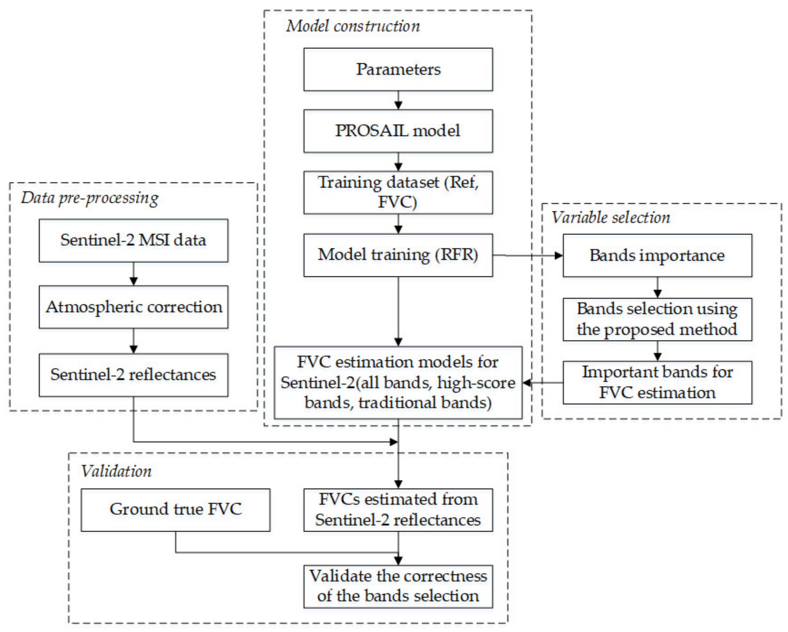
2. Materials and Methods

The flow chart of the proposed method to assess Sentinel-2 MSI reflectances for estimating FVC in this study is shown in Figure 1. The basic parts of the method include data pre-processing, model construction, variable selection and validation.

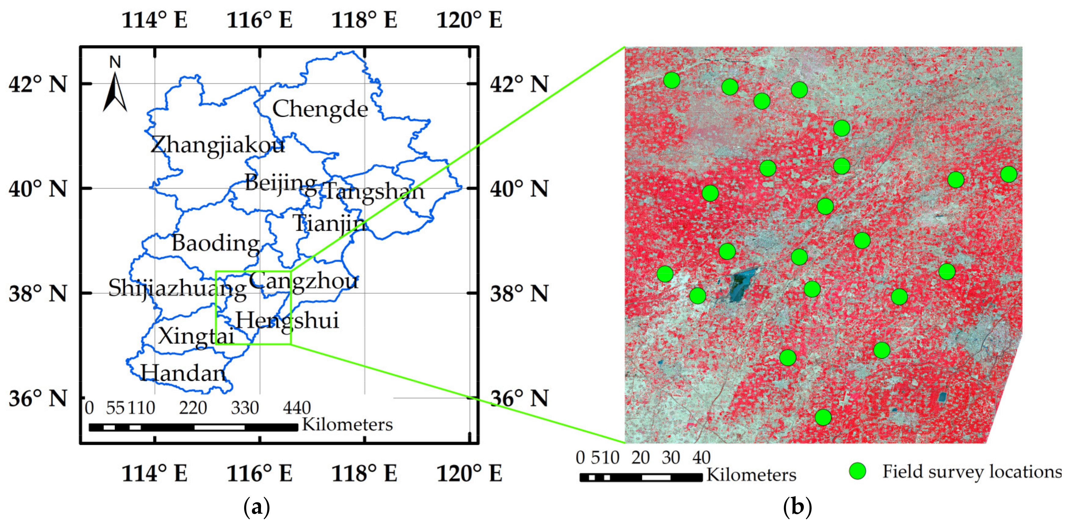
2.1. Study Area and Field Survey

The study area is located in Hengshui (115°10′E~116°34′E, 37°03′N~38°23′N) in the southeast of Hebei province, China (Figure 2). The landform is plain, with an altitude varying from 10 m to 30 m. The climate type of the study area is temperate continental monsoon with four obvious seasons. The climate condition is warm, semi-arid, and the annual average precipitation is approximately 509.7 mm. The land cover types are mainly farmland and residential area. The dominant crops are wheat and maize, which account for large percentages of farmland in spring and autumn, respectively [56].
Field FVC measurements were collected twice for wheat and twice for maize on different growing periods, as listed in Table 2. The sample sites were spread over all 11 counties of Hengshui with sizes of 100 m × 100 m. There were two sample sites in each county and a total of 22 sites in the entire study area. The sample sites were located in the middle of relatively homogeneous farmland. Five sample points, with sizes of 30 m × 30 m, were selected for each sample sites, four on the corners and one in the center. Coordinates of each sample point were collected using handheld Global Positioning System (GPS) devices. At each sample point, five photographs were taken using digital cameras, and field FVC data were quantitatively acquired from these photographs. Finally, the average of five FVCs derived from photographs at each sample point was used to validate the FVC estimated from the Sentinel-2 images. Therefore, there were 110 ground truth points (GTPs) for maize or wheat in a survey period. There were two survey periods for maize and wheat, respectively, thus, in theory, 440 GTPs could be used to validate the estimated FVC. However, in practical applications, these points could not all be used due to continuous cloud contamination.
The original photographs were stored in JPEG format with a size of 4000 × 3000 pixels. Twenty-five percent of photo edges were cut to eliminate the influence of the large geometric distortion at the sides of the photograph, which resulted in a subset of photographs representing the survey points [57]. For better FVC extraction, a shadow-resistant algorithm was used to estimate FVC of each photograph in this study [58]. The algorithm introduced hue saturation intensity (HIS) color space to equalize the intensity histogram, enhancing the brightness of shaded parts in the photographs. Lognormal and Gaussian distribution functions were then applied to fit the distributions of green vegetation and background on the green red component in the L*A*B color space. Finally, a threshold value was automatically selected to classify green vegetation and background. The proportion of green vegetation was considered as the FVC of the photograph.

2.2. Sentinel-2 MSI Data and Preprocessing

The Sentinel-2 product available for users is Level-1C data (https://scihub.copernicus.eu), which refers to top-of-atmosphere reflectances in cartographic geometry in the UTM/WGS84 projection, with a size of 100 km × 100 km. The study area is fully covered by four adjacent Sentienl-2 images (tile numbers 50SLG, 50SLH, 50SMG, and 50SMH). The available images were acquired from 26 March 2017 to 31 August 2017 and covered the entire field survey stage. However, due to the influence of continuous thick clouds, some images were not used for FVC estimation. Images used in this study are listed in Table 3.
The preprocessing of Sentinel-2 images included atmospheric correction, spatial resampling and mosaicking. ESA recommends free open source Sentinel Application Platform (SNAP) toolboxes developed by ESA for scientific exploitation of Sentinel missions. The Sen2Cor algorithm in SNAP toolbox [59], version 2.4.0, was used for atmospheric correction. It eliminates the effects of the atmosphere from Level-1C and delivers the Level-2A product of bottom-of-atmosphere reflectance in cartographic geometry. The bands with 10-m and 20-m spatial resolution were processed. After atmospheric correction, bands with 10-m spatial resolution were resampled to 20 m using bilinear interpolation method, and adjacent images with the same acquisition date were then stitched together.

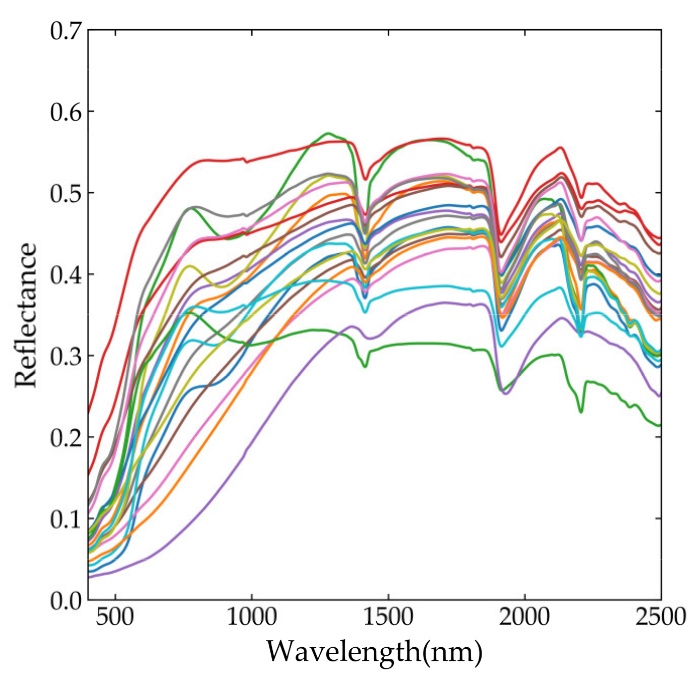
2.3. Generating the Learning Dataset Using the PROSAIL Model

In this study, the PROSAIL model was used to simulate the relationship between Sentinel-2 reflectance and the corresponding FVC. The PROSAIL model is widely used for reflectance modeling due to its good compromise between the process complexity, accuracy and computation time requirements [60]. The model is the combination of the leaf optical properties model PROSPECT and the scattering by arbitrarily inclined leaves (SAIL) canopy reflectance model [55]. The SAIL model is a canopy bidirectional reflectance distribution function model that assumes that the canopy is a turbid medium with randomly distributed leaves [61]. The canopy structure in the SAIL model is characterized by leaf area index (LAI), the average leaf angle inclination (ALA) (with the assumption of an ellipsoidal distribution) and the hot-spot parameter [50]. The input parameters of SAIL include leaf reflectance, leaf transmittance, LAI, soil reflectance (SR), ALA, solar zenith angle (SZA), viewing zenith angle (VZA), hot-spot parameter (Hot), and relative azimuth angle (RAZ).
To compute the FVC simulated by PROSAIL, the classical gap fraction relationships with LAI and ALA were used with the following formulae [62]:
P 0 ( θ ) = e λ 0 G ( θ , θ 1 ) cos θ × L A I
F V C = 1 P 0 ( 0 )
where P0(θ) is the gap fraction, θ is the direction where the gap fraction is computed, G(θ, θ1) is the orthogonal projection of a unit leaf area along direction θ, and θ1 is the ALA. The parameter λ0 is the leaf dispersion or clumping. Because FVC was defined as seen from the nadir direction, the FVC was computed when θ is equal to 0.
The PROSPECT model provides the optical properties of plant leaves from 400 nm to 2500 nm at the leaf level for the purpose of directional-hemispherical reflectance and transmittance simulation [63]. The PROSPECT model is based on the representation of the leaf as one or several absorbing plates with rough surfaces causing isotropic scattering [64]. This study chose the PROSPECT-D version of the model, whose input parameters are leaf structure parameter (N), leaf chlorophyll a + b concentration (Cab), equivalent water thickness (Cw), dry matter content (Cm), carotenoid content (Car), brown pigment content (Cbrown) and anthocyanin content (Cant). To better represent land surface conditions and constraining the inversion process, prior knowledge was added to input parameters of PROSAIL based on previous studies [65,66,67,68,69]. The range and specific distribution of the main input parameters of PROSAIL are listed in Table 4.
The reflectance of soil is also an important parameter for PROSAIL model. In this study, soil reflectances were selected from a globally distributed soil spectral library released by the International Soil and Information Centre (http://data.isric.org/geonetwork/srv/chi/catalog.search# /metadata/1081ac75-78f7-4db3-b8cc-23b78a3aa769). The original soil reflectances, whose locations are distributed across 58 countries spanning Africa, Asia, Europe, North America and South America, contain various soil types with different properties [70]. The original soil reflectances were resampled from an interval of 10 nm to 1 nm by cubic spline functions to conform to the spectral response function of Sentinel-2. Then, the soil reflectances were resampled to correspond to Sentinel-2 spectra using the following formula [71]:
ρ = λ = 1 N β ( λ ) × ρ ( λ ) λ = 1 N β ( λ )
where ρ and ρ ( λ ) are the corresponding simulated Sentinel soil reflectances and resampled soil reflectances, respectively. β(λ) represents the weight of the band’s spectral response function of Sentinel-2 MSI.
To remove data redundancy caused by similar soil reflectances and reduce huge computation in PROSAIL simulation, the spectral angle mapper [72,73] was used to assess the similarity of soil reflectances and further classify the original soil reflectances into several categories. Similar reflectances of each category were averaged as a representative soil reflectance. Considering two spectral vectors with n wavebands, where X = (x1, x2, …, xn) and Y = (y1, y2, …, yn), the spectral angle could be defined as the following:
α X Y = cos 1 [ i = 1 n x i y i ( i = 1 n x i 2 ) 1 / 2 ( i = 1 n y i 2 ) 1 / 2 ]
where X and Y represent two different soil spectral reflectance vectors, αXY is the spectral angle between the two spectral vectors X and Y, and the value range of α is between 0 and π/2. The two spectral vectors are completely similar when α = 0 and completely different when α = π/2; the larger α values indicate greater differences between the two spectral vectors [74]. In this study, if the spectral angle between soil reflectances and central vectors of the corresponding categories was smaller than 0.05, it was considered as a similar soil reflectance. The final 20 soil reflectances derived from original soil reflectances were used to represent the possible range of soil spectral reflectances (Figure 3).
The input parameters of the PROSAIL model were randomly generated using the specific distribution and range of each parameter every time, and the top of canopy reflectances were then simulated for each wavelength by the PROSAIL model and resampled to simulate the specific band reflectances of Sentinel-2 using Formula (3). Considering uncertainties attached to the sensor measurements and models, a white Gaussian noise of 1% was added to the simulated reflectances [50]. Because the three bands with 60-m spatial resolution were mainly dedicated to atmospheric correction and cloud screening, they were removed in the simulated dataset. According to the previous studies [71,75], and considering the computational efficiency, a medium quantity dataset that contained 200,000 items was simulated, of which 80% were randomly selected as the training dataset and the remaining 20% were used for validation.

2.4. Random Forest Regression

Random forests are one of the most popular machine learning methods for both classification and regression. RFR is an ensemble of regression trees, which are often binary decision trees (CART), and the average of predictions from the individual trees is the prediction result of the forest. The main advantages of RFR are that they do not overfit as more trees are added but always produce a limited value of the generalization error and are more robust to noise data. In the case where the dimension is comparable or larger than the sample size, RFR can still achieve satisfactory performance [76]. Random forests use two aspects of the random property: each tree is grown from an independent bootstrap sample of the data and randomly choosing a subset of explanatory variables at each node of the tree as candidate variables to split on. The number of input variables randomly chosen at each split mtry and the number of trees in the forest ntree are the two main parameters of random forests [76]. In this study, mtry was set to the square root (or 1/3) of the total number of bands (i.e., 3 bands) and ntree was set to 500; these settings are similar to other studies [76,77].
In this study, RFR was selected for FVC estimation. The simulated Sentinel-2 MSI band reflectances of the training dataset were used as the inputs and the outputs were the corresponding FVC. The RFR was trained using the training dataset and then used to build the relationship between band reflectances and FVC. The validation dataset was used to validate the prediction accuracy and generalization.

2.5. Variables Importance and Selection

Generally speaking, the variable selection procedure includes two steps: (1) ranking the variables based on importance scores; and (2) determining a sufficient subset for prediction [77]. In the RF framework for regression problems, increasing Mean Squared Error (MSE) is widely used to evaluate the importance score of a given variable, when the observed values of this variable are randomly permuted in the Out-of-Bag samples (OOB), and variable importance is determined based on the measure [76]. The OOB for a tree is the set of observations that are not used for building the current tree, which accounts for 1/e 36.8% of the observations.
After determining the importance scores of variables, all variables are ranked as a sequence based on them. The most critical issue comes next: determining the number of variables to be selected. In this study, the following strategy was proposed to solve the problem. The strategy starts with the most important band based on the importance scores and then progressively adds the most important of the remaining bands. At each iteration (n = 10), the root mean square error (RMSE) of the prediction model is calculated. If the band added caused significant reduction in RMSE, the band is important and has great influence on improving the accuracy of FVC estimation. In contrast, if the RMSE did not reduce the RSME or improve the FVC estimation significantly, the band is redundant. Conventionally, if a band has a high importance score and ranks ahead of the sequence of bands, it should cause an obvious reduction in RMSE, and the band with low importance score should not.
The assessment of band importance score was based on the simulated data generated by PROSAIL model, and this process was carried out simultaneously with the FVC estimation. In this study, firstly, all 10 simulated band reflectances were used to establish the RFR model and assess the importance of different bands. Then, the most important bands were selected to reestablish the RFR model, and the FVC prediction result of both simulated data and real Sentinel-2 band reflectances were compared separately between these two models to investigate the efficiency of band selection. Another experiment that combined red, green and NIR band reflectances as the inputs, provided by some multispectral sensors with only four bands such as SPOT, Chinese GF-1 and GF-2, was also conducted.

3. Results

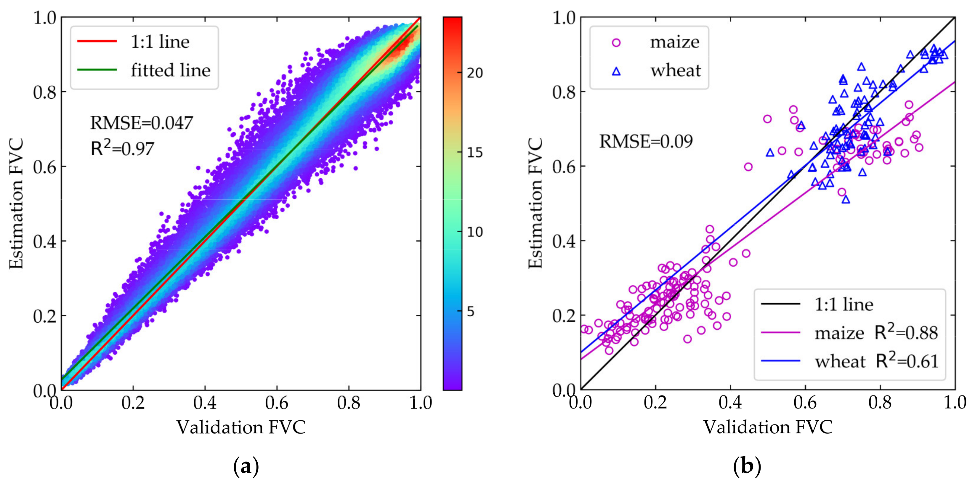
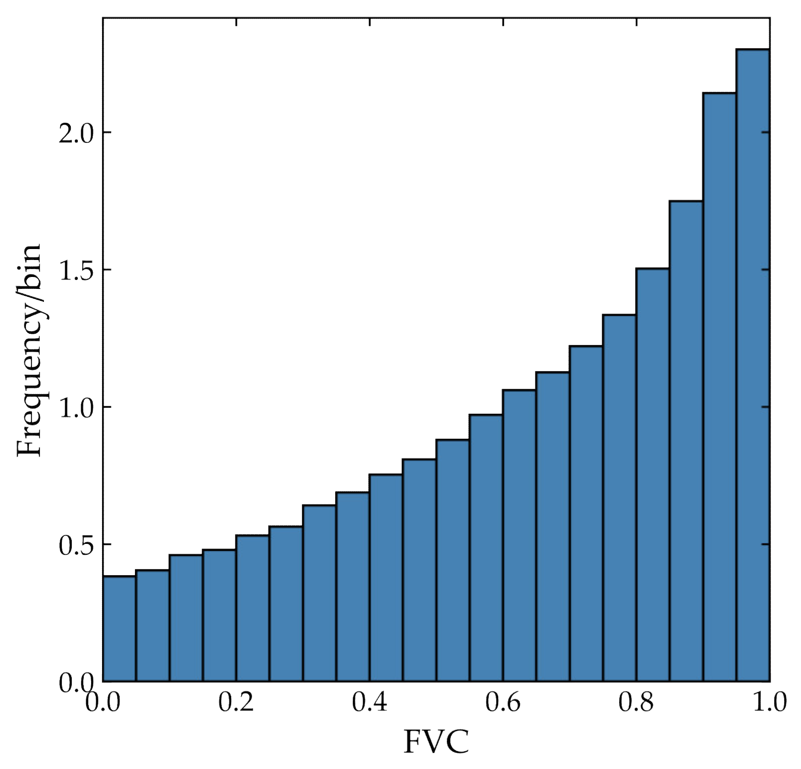
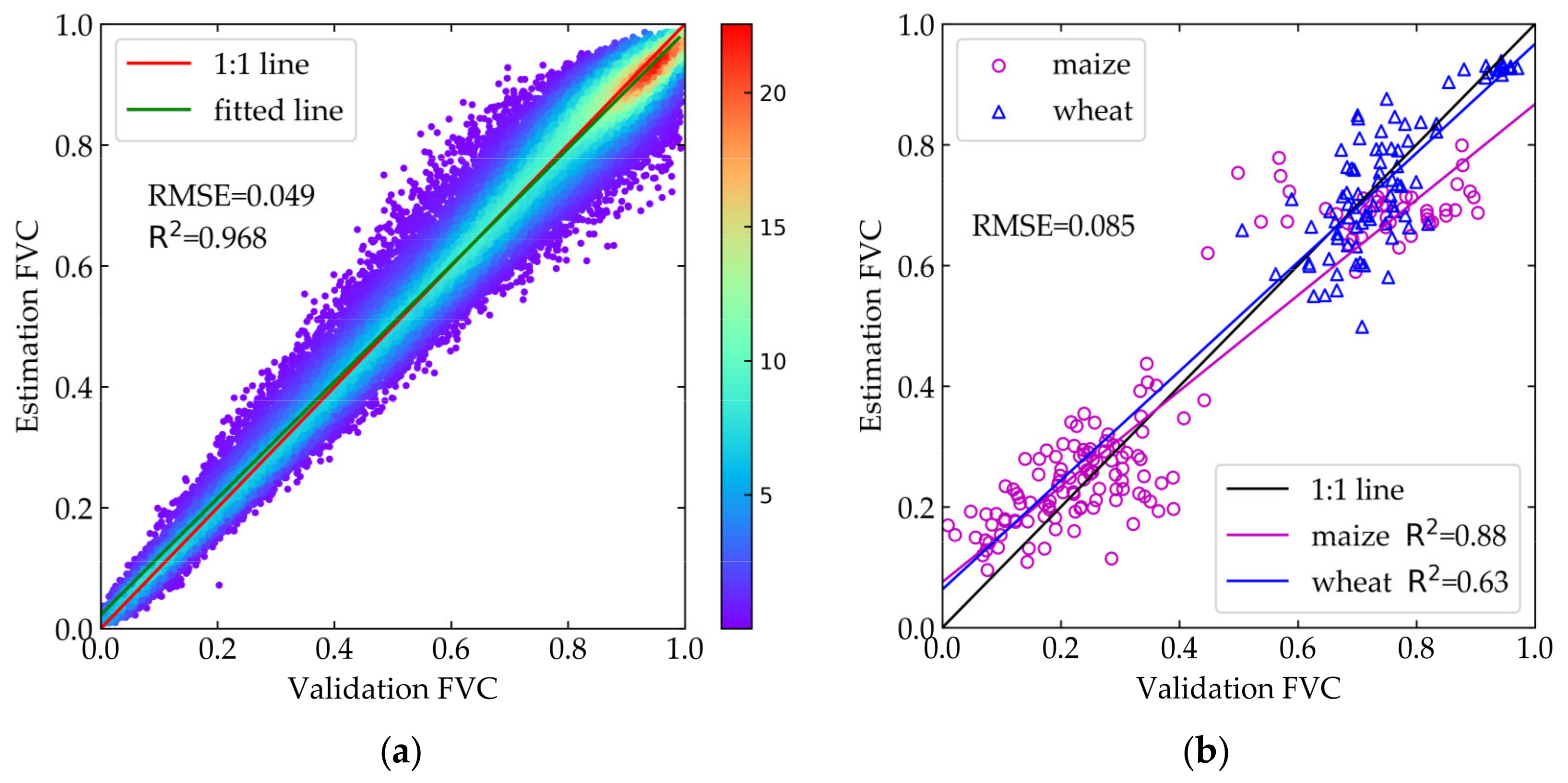
3.1. Estimating FVC Using 10 Bands of Sentinel-2 MSI Data

Figure 4a shows the FVC estimation results using the simulated validation data. The FVC estimation accuracy based on the simulated validation data shows reliable performance (RMSE = 0.047 and R2 = 0.97). The distribution of the most scattered points is basically located around the 1:1 line, and the closer to the 1:1 line, the greater the density. Few points are scattered a little far from the 1:1 line, but these points only account for a small proportion of the total number of points, and the point density is also small. The fitted line is almost parallel to the 1:1 line. For the specific Gaussian distribution of LAI and the relationship between LAI and FVC, the distribution of FVC in the simulated data is shown in Figure 5. The average simulated reflectance spectra are shown in Figure 6. These results demonstrate that the dataset generated by PROSAIL model has a lot of variability and can adapt to most conditions of land surface. The validation performance based on the simulated data indicates that the RFR model is reliable and has good generalization ability to adapt to various situations.
Figure 4b shows the accuracy of FVC estimated from Sentinel-2 MSI band reflectances using the RFR model validated by the field FVC measurement. The magenta circles represent the maize survey points, and the blue triangles represent the wheat survey point. Due to different growth periods, FVC values of wheat and maize were distributed in different ranges, but, within one ground survey period, the FVC values vary within a small range among one class. Thus, it seems that they fell into different clumps. For cloud cover and satellite revisit cycle issues, a linear interpolation method was applied using FVC estimated from Sentinel-2 reflectances of two phases before and after the field survey dates to obtain FVC at the dates corresponding to the field survey. However, the locations of some sample points were covered by clouds on all images. As a result, the number of field survey FVC used to validate FVC estimates was often less than the total number of sample points. The RMSE using all field survey points is 0.09, which is reasonable for FVC estimation. The R2 of maize is 0.88, which is higher than wheat (0.61). Therefore, the validation result indicates that the trained RFR model is robust and can be used to estimate FVC and assess the importance of Sentinel-2 MSI band reflectances for FVC estimation.

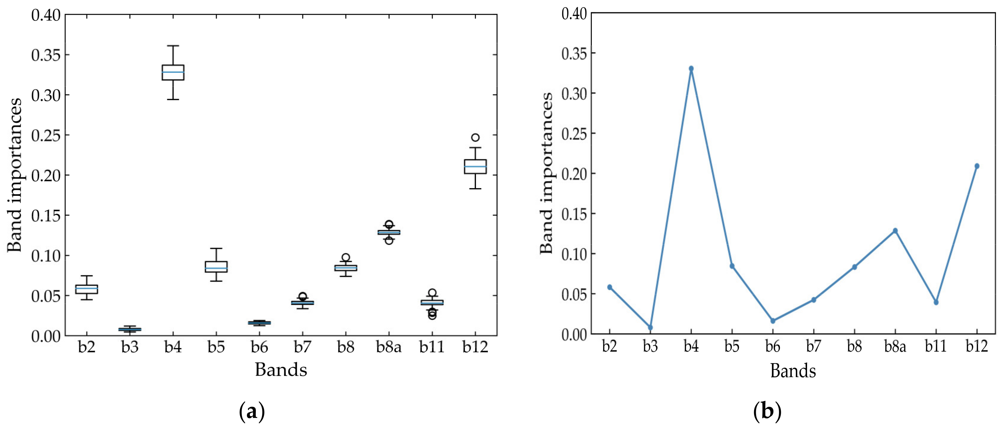
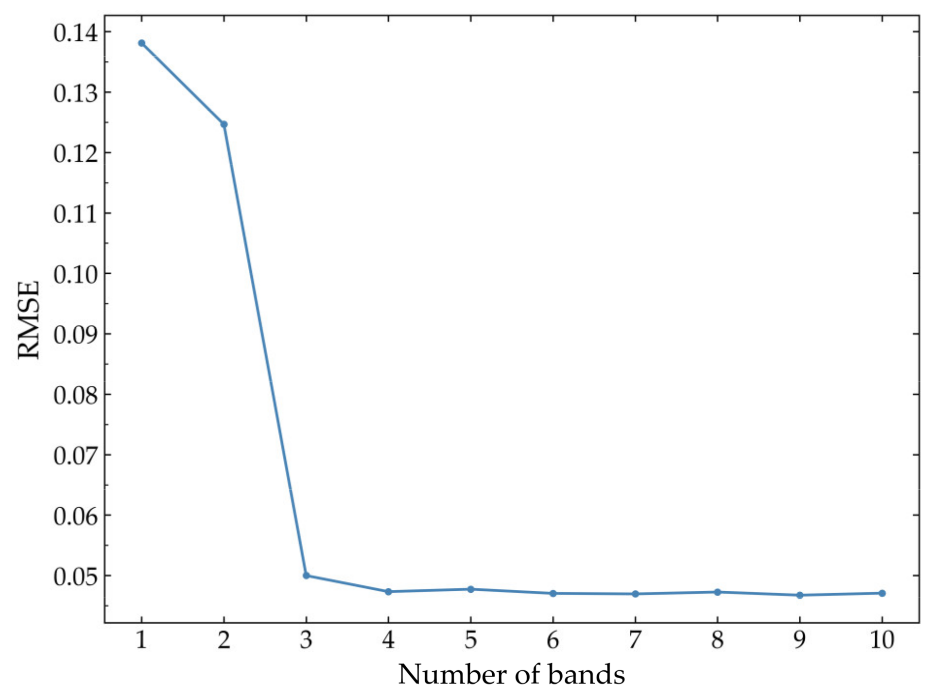
3.2. Bands Importance Evaluation and Selection

Figure 7a shows the boxplot of the band importance scores over 50 trials with training set randomly split by 80% of the total simulated data every time, and Figure 7b shows the average value. The result obviously shows that band 4, which refers to the red band, is the most important band and its important score is much higher than the other bands. This means that the red band reflectance contains much more useful information for FVC estimation compared to other bands. In terms of green plants, incident radiation is mainly assimilated by chlorophylls at red and blue spectral regions with central wavelengths of 0.45 μm and 0.65 μm, respectively. However, a reflectance peak occurs at the green spectral region with a central wavelength of 0.54 μm [78]. The strong reflectance peak at the green band accounts for the green color perceived by human eyes and distinguishes the green plant component from the background. Figure 8 shows high correlations with correlation coefficients greater than 0.86 among red, green, blue and RE1 band reflectances. Many studies had proven that in RFR model, when several highly correlated variables exist for a certain variable, its variable importance will decrease [76,77], while this high correlation has no significant influence in importance levels of the other variables. More importantly, the important variables cannot be confused with noise. Red band reflectance for FVC estimation is more important than green, blue and RE1 band reflectances, so the importance scores of later three bands should decrease to some extent.
A striking contrast is that the score of SWIR2 band is the second highest among all bands, while that of SWIR1 band is relatively low. The SWIR spectral region ranges from 1.4 μm to 2.5 μm and is affected by leaf liquid water [79]. The SWIR2 band can be used to distinguish vegetation from soil. For example, Asner et al. proposed a biogeophysical approach for the unmixing of soils and vegetation using SWIR band between 2.1 μm and 2.5 μm spectral regions in arid and semiarid ecosystems [80]. It is demonstrated that band 12, with a central wavelength of 2.19 μm, has a very powerful potential for FVC estimation. Therefore, band 12 is much more important than band 11 for FVC estimation because band 11 with a central wavelength of 1.61 μm is out of the spectral range. SWIR1 and SWIR2 band reflectances also have a high correlation with a correlation coefficient of 0.9 (Figure 8). The SWIR1 band with a central wavelength of 1.61 μm is helpful for vegetation information extraction like nitrogen content [81], but, as mentioned above, SWIR2 band is better than SWIR1 band for FVC estimation, thus the SWIR1 band is treated as noise by RFR model, which in turn is given a very low score.
The phenomenon in which the band reflectances are highly correlated also occurs in the NIR spectral region, including band 6, band 7, band 8 and band 8a, whose correlation coefficients are greater than 0.8 (Figure 8). NIR bands are usually considered to be the important bands to characterize vegetation status and distinguish vegetation from other land cover types because of the high reflectance of vegetation in this spectral range caused by internal scattering and low absorption of leaves [78]. The scores of those band reflectances have some degree of decline due to high correlation between bands, but the NIR2 band reflectance shows the highest importance for FVC estimation among these four bands.
Based on the average of band importance scores over 50 trials, Figure 9 shows the result of the variables selection strategy proposed in this study. The model started only with the most important band, the red band. When SWIR2 and NIR2 bands were added to the RFR model, the RMSE of validating dataset split by 20% of the total simulated data dropped to a large extent. As more and more bands were added to the RFR model in the order of decreasing importance scores for FVC estimation, the RMSE was not significantly reduced. It can be clearly seen that, after three bands were added to the RFR model, the RMSE appeared to be stable with small fluctuations. This indicates that the accuracy of FVC estimation would not be significantly improved even if more bands were added to the RFR model. Instead, more bands added would only add to calculation cost. Therefore, the red, NIR2 and SWIR2 bands were selected as the most important bands for FVC estimation.

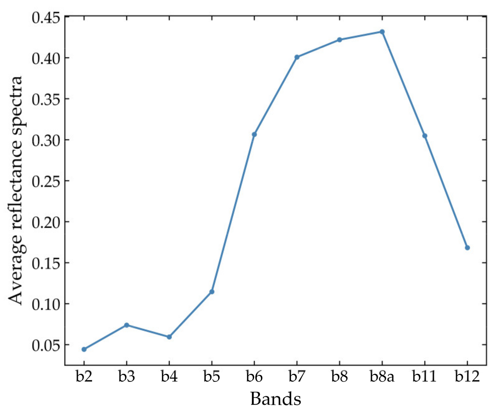
3.3. High-Score Band Reflectances for FVC Estimation

The high-score bands were selected to estimate FVC with simulated validation data and real band reflectances data using RFR model to validate whether they can achieve comparable or better FVC estimation accuracy, and further examine the effectiveness of band selection. The three most important bands selected by RFR model are red, SWIR2 and NIR2 bands. The validation result (RMSE = 0.049 and R2 = 0.968) using the simulated validation data is shown in Figure 10a. The validation accuracy using high-score bands is approximately equal to, and slightly lower than, using all bands, but the difference is almost negligible. The simulated data demonstrate that the band selection method proposed in this study is appropriate. However, compared to the simulated data, real data are more complex and FVC estimation is more difficult. To verify whether the important bands selected by RFR model using simulated data are applicable to real Sentinel-2 band reflectances, field survey FVC data were used to validate the reasonability of band selection. Figure 10b shows the validation result of FVC estimated from the high-score bands of Sentinel-2 reflectances using RFR model by field survey data. The RMSE using all field survey points is 0.085. The R2 of maize is 0.88, which is higher than that of wheat (0.63). The validation accuracy is also approximately equal to using all bands, and slightly higher, but the difference is insignificant. Therefore, the results demonstrate that red, SWIR2 and NIR2 bands are the most important for FVC estimation and the remaining bands have less significant effect on improving the accuracy of FVC estimation. Using the most important bands to estimate FVC can also reduce the amount of data by 1/3 and the accuracy of the FVC estimation will not be reduced due to the data reduction.
To further determine the reasonability of the band selection result, based on simulated reflectances and corresponding FVC, four spectral bands were randomly selected out of 10 over 10,000 times, and then they were used to build RFR models and the accuracy of the model was validated by validation data. The distribution of RMSE is shown in Figure 11. The result shows that most RMSEs are greater than 0.05, which account for 95.56%. The RMSE of high-score bands is 0.048, smaller than 0.05, which implies that using high-score bands to estimate FVC is more effective than most randomly selected bands. The result shows that not all combinations of four bands can achieve good accuracy with small RMSE. When the randomly selected band combination contains high-score bands, the RMSE will be smaller, and most band combinations whose RMSEs are smaller than 0.05 contain all three high-score bands. The result demonstrates that the three high-score bands are indeed the most important bands for FVC estimation.

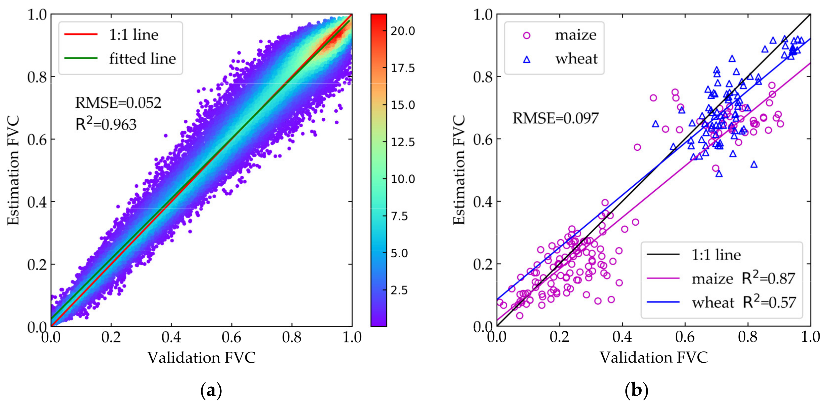
3.4. Comparison with Red, Green and NIR Band Reflectances for FVC Estimation

Some multi-spectral sensors were only equipped with three visible bands and a near-infrared band. Therefore, a comparative validation between these bands and high score bands for FVC estimation was conducted. The red, green and NIR2 bands of the Sentinel-2 MSI band reflectances were selected to estimate FVC using the RFR model. Figure 12a shows the model performance based on the simulated validation data (RMSE = 0.052 and R2 = 0.962). The accuracy is lower than the result using three most important bands.
For the real Sentinel-2 band reflectances, the accuracy validated by field survey data is shown in Figure 12b. The FVC estimation using these three band reflectances shows a lower accuracy. The RMSE using all field survey points is 0.097, the R2 of maize is 0.87 and wheat is 0.57, lower than using the three most important bands. Only SWIR2 band was replaced by the green band as the input bands but there was a clear decrease in FVC estimation accuracy. The result demonstrates that the SWIR2 band has great significance for FVC estimation and can obviously improve FVC estimation accuracy. It can be seen in Figure 7 that green band gets a low score while SWIR2 band gets the second highest score. The result indicates that green band reflectance for FVC estimation is not as effective as SWIR2 band.

4. Discussion

This study proposed a method to assess the importance of Sentinel-2 MSI spectral band reflectances for estimating FVC. The RFR model was trained using the simulated Sentinel-2 reflectances and corresponding FVC, which could give a score for each band reflectance to represent the importance degree for FVC estimation. Band 4, band 8a and band 12 were determined as the three most important bands by variable selection method based on the scores given by RFR model. The selected bands achieved satisfied FVC estimation accuracy by validating using both simulated data and field survey data compared to those using all the bands. In addition, band 12 was found to have the potential to improve FVC estimation accuracy.
In prior studies, several methods have been developed to improve the accuracy of FVC estimation, such as empirical methods, pixel unmixing models and physical based models. However, most studies ignore which spectral information really benefits FVC estimation. This study gave primary insight into which band reflectances of Sentinel-2 mainly contributed to the FVC estimation.
In this study, the performance of band reflectances selection for FVC estimation was evaluated using field survey data. Compared to the simulated data, the accuracy of FVC estimation from real Sentinel-2 band reflectances validated by the field survey FVC data is lower. This phenomenon is normal because simulated data are a simplification of the real world, and the reflectances simulated by the CRTM could not fully match the real reflectances either. Because real band reflectances and field survey data contain uncertainties and variabilities, the accuracy of FVC estimated from the real reflectances is reasonable. For high-score band on FVC estimation, the results of simulated data are consistent with the results of real reflectances and field survey data, that is, whether simulated data or real reflectances and field survey data, using the high-score band reflectances can achieve almost the same or better FVC estimation accuracy compared to using all bands.
The importance scores of band reflectances are influenced by high correlations, and some band reflectances get low scores. However, this is helpful for eliminating band redundancy, which is one of the purposes of variable selection. On the other hand, the fact that these band reflectances got such low scores is not entirely due to correlations. These band reflectances are actually not as important as the band reflectances with high scores for FVC estimation. The result of band importance assessment demonstrates that red, SWIR2 and NIR2 band reflectances are more effective than RE band reflectances for FVC estimation. As for RE band transforms, such as the REPI and red-edge vegetation index (REVI), their potential for FVC estimation is not clear, which will be the future work of this study. Considering the results of band selection, these three bands also equipped in Landsat sensor, whether Sentinel-2 is beneficial over Landsat for FVC estimation remains to be further studied.
This study chose RFR model to assess the Sentinel-2 MSI spectral band reflectances for FVC estimation. However, various ML algorithms can be used to assess variable importance and estimate FVC, such as support vector regression (SVR) [51] and classification and regression trees (CART) [82]. The performance of other ML algorithms remains to be further studied. The VIs are considered as the useful predictors for FVC estimation, such as NDVI, SAVI, transformed soil adjusted vegetation index (TSAVI) [83], and EVI. It is worth exploring the potential of these VIs calculated from Sentinel-2 MSI band reflectances for FVC estimation.

5. Conclusions

The combination of random forest regression and the radiative transfer model was proposed to assess the effects of Sentinel-2 MSI band reflectances on FVC estimation. The field survey FVC data were used to validate the applicability and the FVC estimation results of the established model. The results indicate that various bands had different effects on FVC estimation: the Red, SWIR2 and NIR2 bands of Sentinel-2 MSI data selected by the RFR model were the most important bands and achieved good performance in FVC estimation. The other bands, including the three newly added RE bands, had little effect on improving FVC estimation accuracy, when the three most important bands were used for FVC estimation. Compared with visible and near infrared bands, band 12 of Sentinel-2 MSI data has great potential for improving FVC estimation accuracy. Further work will focus on the potential of REIP and VIs calculated from Sentinel-2 MSI band reflectance for FVC estimation.

Author Contributions

Conceptualization, K.J.; Investigation, B.W. and K.J.; Methodology, B.W. and K.J.; Resources, K.J. and X.X.; Validation, B.W.; Writing—original draft, B.W.; and Writing—review and editing, B.W., K.J., S.L., X.W., X.Z. (Xiang Zhao), Y.Y. and X.Z. (Xiaotong Zhang).

Funding

This research was funded by the National Natural Science Foundation of China (No. 41671332) and the National Key Research and Development Program of China (Nos. 2016YFB0501404 and 2016YFA0600103).

Acknowledgements

The authors would like to thank the anonymous reviewers and editors for their valuable comments and suggestions that have significantly improved this paper. Sentinel-2 data were downloaded from the ESA’s Copernicus Open Access Hub.

Conflicts of Interest

The authors declare no conflict of interest.

References

  1. Purevdorj, T.S.; Tateishi, R.; Ishiyama, T.; Honda, Y. Relationships between percent vegetation cover and vegetation indices. Int. J. Remote Sens. 1998, 19, 3519–3535. [Google Scholar] [CrossRef]
  2. Gitelson, A.A.; Kaufman, Y.J.; Stark, R.; Rundquist, D. Novel algorithms for remote estimation of vegetation fraction. Remote Sens. Environ. 2002, 80, 76–87. [Google Scholar] [CrossRef] [Green Version]
  3. Zhang, X.; Liao, C.; Li, J.; Sun, Q. Fractional vegetation cover estimation in arid and semi-arid environments using hj-1 satellite hyperspectral data. Int. J. Appl. Earth Obs. Geoinf. 2013, 21, 506–512. [Google Scholar] [CrossRef]
  4. Gutman, G.; Ignatov, A. The derivation of the green vegetation fraction from noaa/avhrr data for use in numerical weather prediction models. Int. J. Remote Sens. 1998, 19, 1533–1543. [Google Scholar] [CrossRef]
  5. Zeng, X.; Dickinson, R.E.; Walker, A.; Shaikh, M.; DeFries, R.S.; Qi, J. Derivation and evaluation of global 1-km fractional vegetation cover data for land modeling. J. Appl. Meteorol. 2000, 39, 826–839. [Google Scholar] [CrossRef]
  6. Zhang, X.; Liu, X.; Zhang, M.; Dahlgren, R.A.; Eitzel, M. A review of vegetated buffers and a meta-analysis of their mitigation efficacy in reducing nonpoint source pollution. J. Environ. Qual. 2010, 39, 76–84. [Google Scholar] [CrossRef] [PubMed]
  7. Vinukollu, R.K.; Wood, E.F.; Ferguson, C.R.; Fisher, J.B. Global estimates of evapotranspiration for climate studies using multi-sensor remote sensing data: Evaluation of three process-based approaches. Remote Sens. Environ. 2011, 115, 801–823. [Google Scholar] [CrossRef]
  8. Yang, J.; Weisberg, P.J.; Bristow, N.A. Landsat remote sensing approaches for monitoring long-term tree cover dynamics in semi-arid woodlands: Comparison of vegetation indices and spectral mixture analysis. Remote Sens. Environ. 2012, 119, 62–71. [Google Scholar] [CrossRef]
  9. Torres-Sánchez, J.; Peña, J.M.; de Castro, A.I.; López-Granados, F. Multi-temporal mapping of the vegetation fraction in early-season wheat fields using images from uav. Comput. Electron. Agric. 2014, 103, 104–113. [Google Scholar] [CrossRef]
  10. Ruiz-Colmenero, M.; Bienes, R.; Eldridge, D.J.; Marques, M.J. Vegetation cover reduces erosion and enhances soil organic carbon in a vineyard in the central Spain. Catena 2013, 104, 153–160. [Google Scholar] [CrossRef]
  11. Liang, S.; Li, X.; Wang, J. Advanced Remote Sensing: Terrestrial Information Extraction and Applications; Academic Press: Cambridge, MA, USA, 2012. [Google Scholar]
  12. Zribi, M.; Le Hégarat-Mascle, S.; Taconet, O.; Ciarletti, V.; Vidal-Madjar, D.; Boussema, M.R. Derivation of wild vegetation cover density in semi-arid regions: Ers2/sar evaluation. Int. J. Remote Sens. 2003, 24, 1335–1352. [Google Scholar] [CrossRef]
  13. McGwire, K.; Minor, T.; Fenstermaker, L. Hyperspectral mixture modeling for quantifying sparse vegetation cover in arid environments. Remote Sens. Environ. 2000, 72, 360–374. [Google Scholar] [CrossRef]
  14. Ding, Y.; Zhang, H.; Li, Z.; Xin, X.; Zheng, X.; Zhao, K. Comparison of fractional vegetation cover estimations using dimidiate pixel models and look-up table inversions of the prosail model from landsat 8 oli data. J. Appl. Remote Sens. 2016, 10, 036022. [Google Scholar] [CrossRef]
  15. Li, L.; Yan, G.; Mu, X.; Liu, S.; Chen, Y.; Yan, K.; Luo, J.; Song, W. Estimation of fractional vegetation cover using mean-based spectral unmixing method. In Proceedings of the 2017 IEEE International Geoscience and Remote Sensing Symposium (IGARSS), Fort Worth, TX, USA, 23–28 July 2017; pp. 3178–3180. [Google Scholar]
  16. Horler, D.N.H.; Dockray, M.; Barber, J. The red edge of plant leaf reflectance. Int. J. Remote Sens. 1983, 4, 273–288. [Google Scholar] [CrossRef]
  17. Defries, R.S.; Townshend, J.R.G. Ndvi-derived land cover classifications at a global scale. Int. J. Remote Sens. 1994, 15, 3567–3586. [Google Scholar] [CrossRef]
  18. Huete, A.R. A soil-adjusted vegetation index (savi). Remote Sens. Environ. 1988, 25, 295–309. [Google Scholar] [CrossRef]
  19. Carlson, T.N.; Ripley, D.A. On the relation between ndvi, fractional vegetation cover, and leaf area index. Remote Sens. Environ. 1997, 62, 241–252. [Google Scholar] [CrossRef]
  20. Leprieur, C.; Verstraete, M.M.; Pinty, B. Evaluation of the performance of various vegetation indices to retrieve vegetation cover from avhrr data. Remote Sens. Rev. 1994, 10, 265–284. [Google Scholar] [CrossRef]
  21. Filella, I.; Penuelas, J. The red edge position and shape as indicators of plant chlorophyll content, biomass and hydric status. Int. J. Remote Sens. 1994, 15, 1459–1470. [Google Scholar] [CrossRef]
  22. Clevers, J.G.P.W.; Gitelson, A.A. Remote estimation of crop and grass chlorophyll and nitrogen content using red-edge bands on sentinel-2 and -3. Int. J. Appl. Earth Obs. Geoinf. 2013, 23, 344–351. [Google Scholar] [CrossRef]
  23. Boochs, F.; Kupfer, G.; Dockter, K.; KÜHbauch, W. Shape of the red edge as vitality indicator for plants. Int. J. Remote Sens. 1990, 11, 1741–1753. [Google Scholar] [CrossRef]
  24. Ramoelo, A.; Cho, M.A.; Mathieu, R.; Madonsela, S.; van de Kerchove, R.; Kaszta, Z.; Wolff, E. Monitoring grass nutrients and biomass as indicators of rangeland quality and quantity using random forest modelling and worldview-2 data. Int. J. Appl. Earth Obs. Geoinf. 2015, 43, 43–54. [Google Scholar] [CrossRef]
  25. Cho, M.A.; Skidmore, A.K. A new technique for extracting the red edge position from hyperspectral data: The linear extrapolation method. Remote Sens. Environ. 2006, 101, 181–193. [Google Scholar] [CrossRef]
  26. Cho, M.A.; Skidmore, A.K.; Atzberger, C. Towards red-edge positions less sensitive to canopy biophysical parameters for leaf chlorophyll estimation using properties optique spectrales des feuilles (prospect) and scattering by arbitrarily inclined leaves (sailh) simulated data. Int. J. Remote Sens. 2008, 29, 2241–2255. [Google Scholar] [CrossRef]
  27. Kross, A.; McNairn, H.; Lapen, D.; Sunohara, M.; Champagne, C. Assessment of rapideye vegetation indices for estimation of leaf area index and biomass in corn and soybean crops. Int. J. Appl. Earth Obs. Geoinf. 2015, 34, 235–248. [Google Scholar] [CrossRef]
  28. Karlson, M.; Ostwald, M.; Reese, H.; Bazié, H.R.; Tankoano, B. Assessing the potential of multi-seasonal worldview-2 imagery for mapping west african agroforestry tree species. Int. J. Appl. Earth Obs. Geoinf. 2016, 50, 80–88. [Google Scholar] [CrossRef]
  29. Asadzadeh, S.; de Souza Filho, C.R. Investigating the capability of worldview-3 superspectral data for direct hydrocarbon detection. Remote Sens. Environ. 2016, 173, 162–173. [Google Scholar] [CrossRef]
  30. Drusch, M.; Del Bello, U.; Carlier, S.; Colin, O.; Fernandez, V.; Gascon, F.; Hoersch, B.; Isola, C.; Laberinti, P.; Martimort, P.; et al. Sentinel-2: Esa’s optical high-resolution mission for gmes operational services. Remote Sens. Environ. 2012, 120, 25–36. [Google Scholar] [CrossRef]
  31. Matsushita, B.; Yang, W.; Chen, J.; Onda, Y.; Qiu, G. Sensitivity of the enhanced vegetation index (evi) and normalized difference vegetation index (ndvi) to topographic effects: A case study in high-density cypress forest. Sensors 2007, 7, 2636–2651. [Google Scholar] [CrossRef]
  32. Jiang, Z.; Huete, A.R.; Didan, K.; Miura, T. Development of a two-band enhanced vegetation index without a blue band. Remote Sens. Environ. 2008, 112, 3833–3845. [Google Scholar] [CrossRef]
  33. Wang, C.; Chen, J.; Wu, J.; Tang, Y.; Shi, P.; Black, T.A.; Zhu, K. A snow-free vegetation index for improved monitoring of vegetation spring green-up date in deciduous ecosystems. Remote Sens. Environ. 2017, 196, 1–12. [Google Scholar] [CrossRef]
  34. Grömping, U. Variable importance assessment in regression: Linear regression versus random forest. Am. Stat. 2009, 63, 308–319. [Google Scholar] [CrossRef]
  35. Breiman, L. Random forests. MLear 2001, 45, 5–32. [Google Scholar] [CrossRef]
  36. Rodriguez-Galiano, V.F.; Chica-Olmo, M.; Abarca-Hernandez, F.; Atkinson, P.M.; Jeganathan, C. Random forest classification of mediterranean land cover using multi-seasonal imagery and multi-seasonal texture. Remote Sens. Environ. 2012, 121, 93–107. [Google Scholar] [CrossRef]
  37. Wang, L.A.; Zhou, X.; Zhu, X.; Dong, Z.; Guo, W. Estimation of biomass in wheat using random forest regression algorithm and remote sensing data. Crop J. 2016, 4, 212–219. [Google Scholar] [CrossRef]
  38. Mutanga, O.; Adam, E.; Cho, M.A. High density biomass estimation for wetland vegetation using worldview-2 imagery and random forest regression algorithm. Int. J. Appl. Earth Obs. Geoinf. 2012, 18, 399–406. [Google Scholar] [CrossRef]
  39. Bioucas-Dias, J.M.; Plaza, A.; Dobigeon, N.; Parente, M.; Du, Q.; Gader, P.; Chanussot, J. Hyperspectral unmixing overview: Geometrical, statistical, and sparse regression-based approaches. IEEE J. Sel. Top. Appl. Earth Obs. Remote Sens. 2012, 5, 354–379. [Google Scholar] [CrossRef]
  40. Guerschman, J.P.; Hill, M.J.; Renzullo, L.J.; Barrett, D.J.; Marks, A.S.; Botha, E.J. Estimating fractional cover of photosynthetic vegetation, non-photosynthetic vegetation and bare soil in the australian tropical savanna region upscaling the eo-1 hyperion and modis sensors. Remote Sens. Environ. 2009, 113, 928–945. [Google Scholar] [CrossRef]
  41. Jiapaer, G.; Chen, X.; Bao, A. A comparison of methods for estimating fractional vegetation cover in arid regions. Agric. For. Meteorol. 2011, 151, 1698–1710. [Google Scholar] [CrossRef]
  42. Ding, Y.; Zheng, X.; Jiang, T. Comparison of fractional vegetation cover estimating methods using in-situ measurements and the prosail model from landsat 8 oli data. In Proceedings of the 2016 IEEE International Geoscience and Remote Sensing Symposium (IGARSS), Beijing, China, 10–15 July 2016; pp. 4351–4354. [Google Scholar]
  43. Xiao, J.; Moody, A. A comparison of methods for estimating fractional green vegetation cover within a desert-to-upland transition zone in central new mexico, USA. Remote Sens. Environ. 2005, 98, 237–250. [Google Scholar] [CrossRef]
  44. Bruno, C.; Frédéric, B.; Marie, W. Improving canopy variables estimation from remote sensing data by exploiting ancillary information. Case study on sugar beet canopies. Agronomie 2002, 22, 205–215. [Google Scholar]
  45. Atzberger, C. Object-based retrieval of biophysical canopy variables using artificial neural nets and radiative transfer models. Remote Sens. Environ. 2004, 93, 53–67. [Google Scholar] [CrossRef]
  46. Darvishzadeh, R.; Skidmore, A.; Schlerf, M.; Atzberger, C. Inversion of a radiative transfer model for estimating vegetation lai and chlorophyll in a heterogeneous grassland. Remote Sens. Environ. 2008, 112, 2592–2604. [Google Scholar] [CrossRef]
  47. Houborg, R.; Fisher, J.B.; Skidmore, A.K. Advances in remote sensing of vegetation function and traits. Int. J. Appl. Earth Obs. Geoinf. 2015, 43, 1–6. [Google Scholar] [CrossRef] [Green Version]
  48. Roujean, J.-L.; Lacaze, R. Global mapping of vegetation parameters from polder multiangular measurements for studies of surface-atmosphere interactions: A pragmatic method and its validation. J. Geophys. Res. Atmos. 2002, 107, ACL–6. [Google Scholar] [CrossRef]
  49. Bacour, C.; Baret, F.; Béal, D.; Weiss, M.; Pavageau, K. Neural network estimation of lai, fapar, fcover and lai×cab, from top of canopy meris reflectance data: Principles and validation. Remote Sens. Environ. 2006, 105, 313–325. [Google Scholar] [CrossRef]
  50. Baret, F.; Hagolle, O.; Geiger, B.; Bicheron, P.; Miras, B.; Huc, M.; Berthelot, B.; Niño, F.; Weiss, M.; Samain, O.; et al. Lai, fapar and fcover cyclopes global products derived from vegetation: Part 1: Principles of the algorithm. Remote Sens. Environ. 2007, 110, 275–286. [Google Scholar] [CrossRef]
  51. Tuia, D.; Verrelst, J.; Alonso, L.; Perez-Cruz, F.; Camps-Valls, G. Multioutput support vector regression for remote sensing biophysical parameter estimation. IEEE Geosci. Remote Sens. Lett. 2011, 8, 804–808. [Google Scholar] [CrossRef]
  52. Schwieder, M.; Leitão, J.P.; Suess, S.; Senf, C.; Hostert, P. Estimating fractional shrub cover using simulated enmap data: A comparison of three machine learning regression techniques. Remote Sens. 2014, 6, 3427–3445. [Google Scholar] [CrossRef]
  53. Campos-Taberner, M.; Moreno-Martínez, Á.; García-Haro, J.F.; Camps-Valls, G.; Robinson, P.N.; Kattge, J.; Running, W.S. Global estimation of biophysical variables from google earth engine platform. Remote Sens. 2018, 10, 1167. [Google Scholar] [CrossRef]
  54. Izquierdo-Verdiguier, E.; Zurita-Milla, R. Use of guided regularized random forest for biophysical parameter retrieval. In Proceedings of the IGARSS 2018—2018 IEEE International Geoscience and Remote Sensing Symposium, Valencia, Spain, 22–27 July 2018; pp. 5776–5779. [Google Scholar]
  55. Jacquemoud, S.; Verhoef, W.; Baret, F.; Bacour, C.; Zarco-Tejada, P.J.; Asner, G.P.; François, C.; Ustin, S.L. Prospect+sail models: A review of use for vegetation characterization. Remote Sens. Environ. 2009, 113, S56–S66. [Google Scholar] [CrossRef]
  56. Huang, J.; Tian, L.; Liang, S.; Ma, H.; Becker-Reshef, I.; Huang, Y.; Su, W.; Zhang, X.; Zhu, D.; Wu, W. Improving winter wheat yield estimation by assimilation of the leaf area index from landsat tm and modis data into the wofost model. Agric. For. Meteorol. 2015, 204, 106–121. [Google Scholar] [CrossRef]
  57. Mu, X.; Huang, S.; Ren, H.; Yan, G.; Song, W.; Ruan, G. Validating geov1 fractional vegetation cover derived from coarse-resolution remote sensing images over croplands. IEEE J. Sel. Top. Appl. Earth Obs. Remote Sens. 2015, 8, 439–446. [Google Scholar] [CrossRef]
  58. Song, W.; Mu, X.; Yan, G.; Huang, S. Extracting the green fractional vegetation cover from digital images using a shadow-resistant algorithm (shar-labfvc). Remote Sens. 2015, 7, 10425–10443. [Google Scholar] [CrossRef]
  59. Louis, J.; Debaecker, V.; Pflug, B.; Main-Knorn, M.; Bieniarz, J.; Mueller-Wilm, U.; Cadau, E.; Gascon, F. Sentinel-2 sen2cor: L2a processor for users. In ESA Living Planet Symposium 2016; Ouwehand, L., Ed.; Spacebooks Online: Prague, Czech Republic, 2016; Volume SP-740, pp. 1–8. [Google Scholar]
  60. Atzberger, C.; Richter, K. Spatially constrained inversion of radiative transfer models for improved lai mapping from future sentinel-2 imagery. Remote Sens. Environ. 2012, 120, 208–218. [Google Scholar] [CrossRef]
  61. Verhoef, W. Light scattering by leaf layers with application to canopy reflectance modeling: The sail model. Remote Sens. Environ. 1984, 16, 125–141. [Google Scholar] [CrossRef]
  62. Nilson, T. A theoretical analysis of the frequency of gaps in plant stands. Agric. Meteorol. 1971, 8, 25–38. [Google Scholar] [CrossRef]
  63. Jacquemoud, S.; Baret, F. Prospect: A model of leaf optical properties spectra. Remote Sens. Environ. 1990, 34, 75–91. [Google Scholar] [CrossRef]
  64. Allen, W.A.; Gausman, H.W.; Richardson, A.J.; Thomas, J.R. Interaction of isotropic light with a compact plant leaf. J. Opt. Soc. Am. 1969, 59, 1376–1379. [Google Scholar] [CrossRef]
  65. Scurlock, J.M.O. Worldwide Historical Estimates of Leaf Area Index, 1932–2000; Oak Ridge National Laboratory: Oak Ridge, TN, USA, 2002. [Google Scholar]
  66. Weiss, M.; Baret, F.; Smith, G.J.; Jonckheere, I.; Coppin, P. Review of methods for in situ leaf area index (lai) determination: Part ii. Estimation of lai, errors and sampling. Agric. For. Meteorol. 2004, 121, 37–53. [Google Scholar] [CrossRef]
  67. Feret, J.-B.; François, C.; Asner, G.P.; Gitelson, A.A.; Martin, R.E.; Bidel, L.P.R.; Ustin, S.L.; le Maire, G.; Jacquemoud, S. Prospect-4 and 5: Advances in the leaf optical properties model separating photosynthetic pigments. Remote Sens. Environ. 2008, 112, 3030–3043. [Google Scholar] [CrossRef]
  68. Richter, K.; Atzberger, C.; Vuolo, F.; Urso, G.D. Evaluation of sentinel-2 spectral sampling for radiative transfer model based lai estimation of wheat, sugar beet, and maize. IEEE J. Sel. Top. Appl. Earth Obs. Remote Sens. 2011, 4, 458–464. [Google Scholar] [CrossRef]
  69. Baret, F.; de Solan, B.; Lopez-Lozano, R.; Ma, K.; Weiss, M. Gai estimates of row crops from downward looking digital photos taken perpendicular to rows at 57.5° zenith angle: Theoretical considerations based on 3d architecture models and application to wheat crops. Agric. For. Meteorol. 2010, 150, 1393–1401. [Google Scholar] [CrossRef]
  70. Shepherd, K.D.; Palm, C.A.; Gachengo, C.N.; Vanlauwe, B. Rapid characterization of organic resource quality for soil and livestock management in tropical agroecosystems using near-infrared spectroscopy. Agron. J. 2003, 95, 1314–1322. [Google Scholar] [CrossRef]
  71. Yang, L.; Jia, K.; Liang, S.; Wei, X.; Yao, Y.; Zhang, X. A robust algorithm for estimating surface fractional vegetation cover from landsat data. Remote Sens. 2017, 9, 857. [Google Scholar] [CrossRef]
  72. Dennison, P.E.; Halligan, K.Q.; Roberts, D.A. A comparison of error metrics and constraints for multiple endmember spectral mixture analysis and spectral angle mapper. Remote Sens. Environ. 2004, 93, 359–367. [Google Scholar] [CrossRef]
  73. Jia, K.; Li, Q.Z.; Tian, Y.C.; Wu, B.F.; Zhang, F.F.; Meng, J.H. Accuracy improvement of spectral classification of crop using microwave backscatter data. Spectrosc. Spectr. Anal. 2011, 31, 483–487. [Google Scholar] [CrossRef]
  74. Jia, K.; Liang, S.; Gu, X.; Baret, F.; Wei, X.; Wang, X.; Yao, Y.; Yang, L.; Li, Y. Fractional vegetation cover estimation algorithm for chinese gf-1 wide field view data. Remote Sens. Environ. 2016, 177, 184–191. [Google Scholar] [CrossRef]
  75. Duan, S.-B.; Li, Z.-L.; Wu, H.; Tang, B.-H.; Ma, L.; Zhao, E.; Li, C. Inversion of the prosail model to estimate leaf area index of maize, potato, and sunflower fields from unmanned aerial vehicle hyperspectral data. Int. J. Appl. Earth Obs. Geoinf. 2014, 26, 12–20. [Google Scholar] [CrossRef]
  76. Ben Ishak, A. Variable selection using support vector regression and random forests: A comparative study. Intell. Data Anal. 2016, 20, 83–104. [Google Scholar] [CrossRef]
  77. Genuer, R.; Poggi, J.-M.; Tuleau-Malot, C. Variable selection using random forests. Pattern Recognit. Lett. 2010, 31, 2225–2236. [Google Scholar] [CrossRef] [Green Version]
  78. Knipling, E.B. Physical and physiological basis for the reflectance of visible and near-infrared radiation from vegetation. Remote Sens. Environ. 1970, 1, 155–159. [Google Scholar] [CrossRef]
  79. Tucker, C.J. Remote sensing of leaf water content in the near infrared. Remote Sens. Environ. 1980, 10, 23–32. [Google Scholar] [CrossRef]
  80. Asner, G.P.; Lobell, D.B. A biogeophysical approach for automated swir unmixing of soils and vegetation. Remote Sens. Environ. 2000, 74, 99–112. [Google Scholar] [CrossRef]
  81. Herrmann, I.; Karnieli, A.; Bonfil, D.J.; Cohen, Y.; Alchanatis, V. Swir-based spectral indices for assessing nitrogen content in potato fields. Int. J. Remote Sens. 2010, 31, 5127–5143. [Google Scholar] [CrossRef]
  82. Breiman, L.; Friedman, J.; Stone, C.J.; Olshen, R.A. Classification and Regression Trees; CRC Press: Boca Raton, FL, USA, 1984. [Google Scholar]
  83. Baret, F.; Guyot, G.; Major, D.J. Tsavi: A vegetation index which minimizes soil brightness effects on lai and apar estimation. In Proceedings of the 12th Canadian Symposium on Remote Sensing Geoscience and Remote Sensing Symposium, Vancouver, BC, Canada, 10–14 July 1989; pp. 1355–1358. [Google Scholar]
Figure 1. Flow chart of this study.
Remotesensing 10 01927 g001
Figure 2. Geographic location of the study area: (a) standard false color image from Sentinel-2 illustrates the geographic location of the study area; and (b) the green points represent the locations of sample plots in the study area.
Remotesensing 10 01927 g002
Figure 3. Twenty soil reflectance curves to represent the possible range of soil spectral shapes.
Remotesensing 10 01927 g003
Figure 4. Validation based on simulated validation data (a) and field survey data (b) using all Sentinel-2 MSI band reflectances.
Remotesensing 10 01927 g004
Figure 5. The distribution of FVC in the simulated data generated by PROSAIL simulation.
Remotesensing 10 01927 g005
Figure 6. The average reflectance spectra of all 200,000 simulated Sentinel-2 MSI reflectances.
Remotesensing 10 01927 g006
Figure 7. Importance of Sentinel-2 bands reflectances for FVC estimation evaluated using RFR: (a) the boxplot of 50 trials; and (b) the average value over 50 trials.
Remotesensing 10 01927 g007
Figure 8. The correlation coefficients between every two bands of Sentinel MSI data.
Remotesensing 10 01927 g008
Figure 9. Importance of Sentinel-2 bands for FVC estimation evaluated using RFR.
Remotesensing 10 01927 g009
Figure 10. Validation based on simulated validation data (a) and field survey data (b) using the Sentinel-2 MSI band reflectances that obtain the highest score.
Remotesensing 10 01927 g010
Figure 11. The distribution of RMSE calculated from four bands RFR model over 10,000 times.
Remotesensing 10 01927 g011
Figure 12. Validation based on simulated validation data (a) and field survey data (b) using the Red, Green and NIR2 band reflectances of Sentinel-2 MSI.
Remotesensing 10 01927 g012
Table 1. Sentinel-2 bands defined by ESA.
Bands No.Central Wavelength (nm)Band Width (nm)Spatial Resolution (m)
14432060
24906510
35603510
46653010
57051520
67401520
77852020
884211510
8a8652020
99452060
1013803060
1116109020
12219018020
Table 2. Field FVC survey in Hengshui.
Crop TypeStart TimeEnd TimeNumber of Sample SitesNumber of GTPs
Wheat20 March 20171 April 201722110
Wheat4 May 20176 May 2017
Maize5 July 20178 July 2017
Maize29 July 201731 July 2017
Table 3. The Sentinel-2 images used in this study.
Acquisition TimeSensor TypeTile Numbers
26 March 2017S2A50SLG, 50SLH
28 April 2017S2A50SLG, 50SLH, 50SMG, 50SMH
8 May 2017S2A50SLG, 50SLH, 50SMG, 50SMH
27 June 2017S2A50SLG, 50SLH, 50SMG, 50SMH
12 July 2017S2A50SLG, 50SLH, 50SMG, 50SMH
11 August 2017S2B50SLG, 50SLH, 50SMG, 50SMH
Table 4. Input parameters of the PROSAIL model.
ModelParametersUnitsRange (or Value)DistributionMeanStd.
PROSPECTCabμg/cm220–90Gauss4530
Cmg/cm20.003–0.011Gauss0.0050.005
Carμg/cm24.4---
Cwcm0.005–0.015Uniform--
Cbrown-0–2Gauss0.00.3
Cantμg/cm20---
N-1.2–2.2Gauss1.50.3
SAILLAI-0–7Gauss2.03.0
ALA 30–70Uniform--
SZA 35---
Hot-0.1–0.5Gauss0.20.5

