Extraction of Buildings from Multiple-View Aerial Images Using a Feature-Level-Fusion Strategy


1
College of Geoscience and Surveying Engineering, China University of Mining and Technology (Beijing), Xueyuan Road DING No. 11, Beijing 100083, China
2
Chinese Academy of Surveying and Mapping, Lianhuachixi Road No. 28, Beijing 100830, China
*
Authors to whom correspondence should be addressed.
Remote Sens. 2018, 10(12), 1947; https://0-doi-org.brum.beds.ac.uk/10.3390/rs10121947
Submission received: 27 September 2018
/
Revised: 21 November 2018
/
Accepted: 28 November 2018
/
Published: 4 December 2018
(This article belongs to the Special Issue Remote Sensing based Building Extraction)
Abstract
:Aerial images are widely used for building detection. However, the performance of building detection methods based on aerial images alone is typically poorer than that of building detection methods using both LiDAR and image data. To overcome these limitations, we present a framework for detecting and regularizing the boundary of individual buildings using a feature-level-fusion strategy based on features from dense image matching (DIM) point clouds, orthophoto and original aerial images. The proposed framework is divided into three stages. In the first stage, the features from the original aerial image and DIM points are fused to detect buildings and obtain the so-called blob of an individual building. Then, a feature-level fusion strategy is applied to match the straight-line segments from original aerial images so that the matched straight-line segment can be used in the later stage. Finally, a new footprint generation algorithm is proposed to generate the building footprint by combining the matched straight-line segments and the boundary of the blob of the individual building. The performance of our framework is evaluated on a vertical aerial image dataset (Vaihingen) and two oblique aerial image datasets (Potsdam and Lunen). The experimental results reveal 89% to 96% per-area completeness with accuracy above almost 93%. Relative to six existing methods, our proposed method not only is more robust but also can obtain a similar performance to the methods based on LiDAR and images.
1. Introduction
Buildings, as key urban objects, play an important role in city planning [1,2], disaster management [3,4,5], emergency response [6], and many other application fields [7]. Due to the rapid development of cities and the requirement for up-to-date geospatial information, automatic building detection from high-resolution remote sensing images remains a primary research topic in the communities of computer vision and geomatics. Over the past two decades, a variety of methods have been proposed for automatic building detection. Based on the types of input data sources, the existing automatic building detection methods can be divided into two categories [8]:
Many researchers have reported that multisource-data-based methods perform better than single-source-data-based methods [18,19,20]. This is mainly because multisource-data-based methods use not only the spectral features provided by images but also the height information for the building detection. However, the cost of multisource-data-based methods may be higher than that of single-source-data-based methods. Moreover, with the fast development of multi-camera aerial platforms and dense matching techniques, reliable and accurate Dense Image Matching (DIM) point clouds can be generated from the overlapping aerial images [21]. Under this condition, instead of using multisource remote sensing data, the approach of solely employing aerial images to extract buildings in complex urban scenes is feasible. The building extraction mainly contains building detection and the regularization of the building boundary in this paper. Hence, we first discuss the related works in building detection paradigm only using aerial images and then cover the relevant literature on boundary regularization in the following work.
From the perspective of the photogrammetric processing, the DIM point cloud, DSM and orthophoto data can be generated from original aerial images, and all these data can provide various features for building extraction. According to the sources of the features used in the process of building detection, we distinguish aerial-image-based methods into four groups: methods using features from images (including original aerial images or orthophoto), methods using features from DIM point clouds, methods fusing the features from orthophoto and DSM and methods fusing the features from aerial images and DIM point clouds.
The first two methods mainly make use of the features from either the images or the DIM point clouds to detect buildings. The images mainly contain the spectral features (such as the color, tone, and texture) and spatial features (such as the area and shape). Based on these features, both pixel-based and segment-/object-oriented classification methods are proposed [22,23] for building detection. Because the pixel-based methods have a salt-and-pepper effect, researchers prefer the latter. The methods in [24,25,26] are several examples. However, objects of the same type may appear to have different spectral signatures, whereas different objects may appear to have similar spectral signatures under various background conditions. Therefore, the methods using features from images alone cannot obtain satisfactory performance, particularly in a complex urban scene.
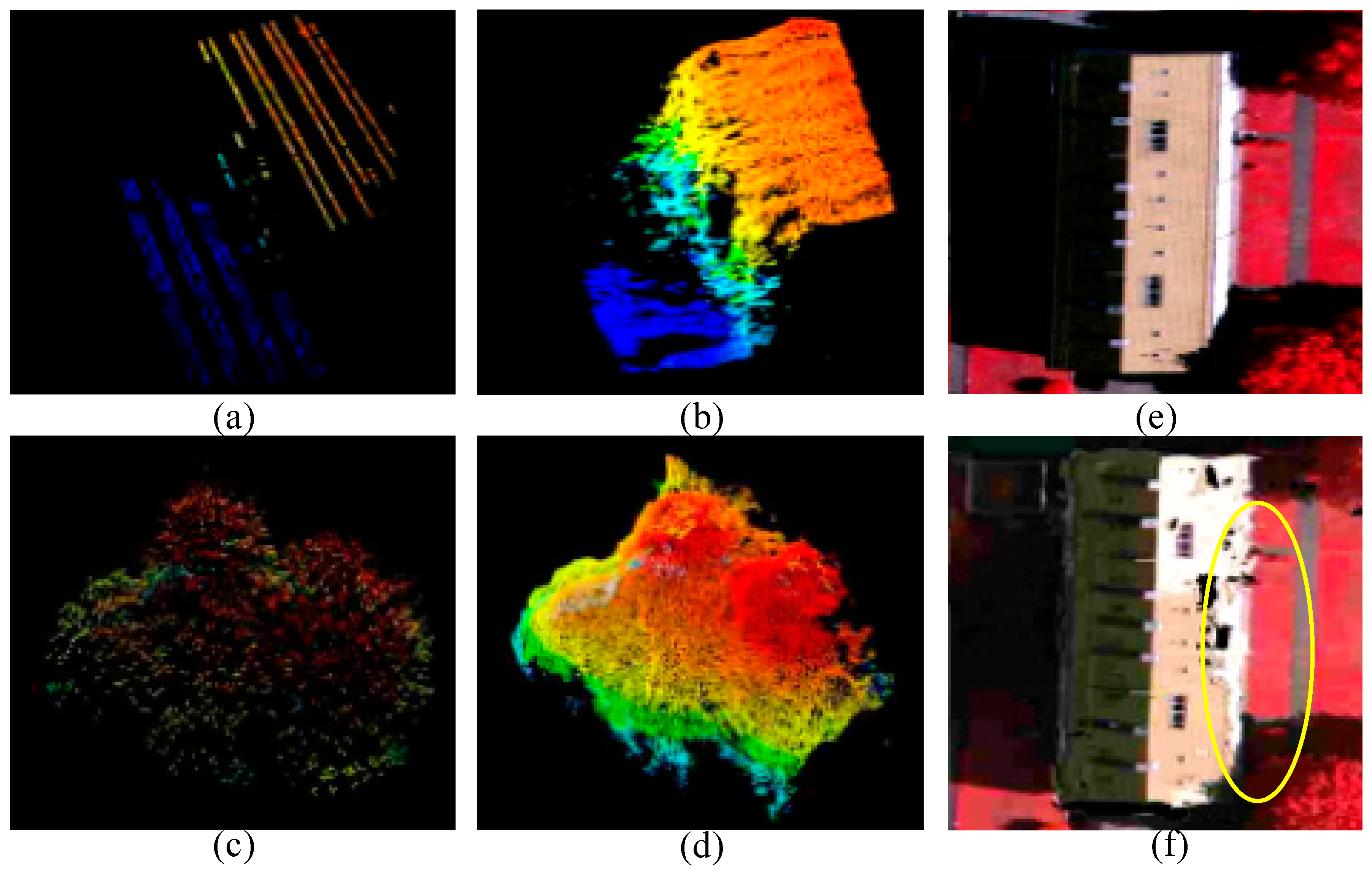
The DIM point clouds mainly provide the height information for buildings detection. Although the cues from DIM point clouds are more robust than the spectral features from images, the 3-Dimensional (3D) shape features of buildings and trees are similar, as shown in Figure 1a–d, which increases the challenges of building detection using DIM point clouds in an urban scenario. In addition, the noise of the DIM point clouds is higher than the ALS data, which causes that the methods based on ALS data for building detection may be not suitable for DIM point clouds. Therefore, compared with the first two methods, the latter two methods are more popular in building detection.
The methods in [27,28,29] are some examples of the methods fusing the features from orthophoto and DSM. Compared with the methods solely using either the spectral information from images or height information from DIM point clouds, the detection results of the methods fusing the features from orthophoto and DSM were more robust and had greater accuracy. However, some disadvantages should not be ignored. On the one hand, compared with the original images, the orthophoto introduces the wrapping phenomenon, as shown in Figure 1e,f. This results that the features from orthophoto, such as texture, cannot reflect the true objects. On the other hand, the DSM, which represent the elevation of the tallest surfaces at that point, is unable to provide the information about the occluded objects such as low buildings. Hence, in terms of the features, the methods fusing the DIM point clouds and original aerial images have more potential for building detection. Our proposed building detection method falls under this category.
Some approaches based on the fusion of DIM point clouds and original aerial images for building detection have been proposed. Xiao et al. [30] makes use of the façade features that are detected from oblique aerial images using edge and height information to extract the buildings first; then, the DIM point cloud is employed to verify the detected buildings. In this method, façades are the most important features, which leads to the situation where the small or low buildings are removed due to the loss of windows on the façades. Rau et al. [31] proposed a method based on a rule hierarchical semantic network. First, this method makes use of a multi-resolution segmentation technique to segment the images into patches and calculate the features of each patch. Subsequently, the object height and gradient features from DIM point clouds and the spectral features from the patch are combined to classify the objects into correct categories. Finally, the DIM point clouds are classified into the correct classes with the aid of back projection. However, this method relies on experience to set the classification thresholds, which severely affected the accuracy of the classification. Second, the method makes use of only nine features to classify the DIM point clouds into five objective categories, resulting in an accuracy of 81% for buildings in National Cheng Kung University (NCKU), Taiwan campus, which is a flat area.
Based on the above analysis, a new building detection method using a feature-level-fusion strategy is proposed in this paper. Specifically,
- Filter the DIM point clouds to get the non-ground points.
- Apply the object-oriented classification method to detect vegetation with the aid of the features from the original aerial images.
- Make use of the back-projection to remove the tree points from the non-ground points so that we can obtain the building DIM points according to classified original aerial images.
- Create the building mask using the building DIM points.
The second task in this paper is the regularization of the building boundary after the building detection. In terms of the boundary regularization, multiple methods [32,33,34,35,36,37,38] have been proposed. Most of these methods are aimed at the LiDAR point clouds. However, the accuracy of the detected boundaries is often compromised due to the point cloud sparsity. In fact, the nature of building boundary regularization is to refine and delineate the boundary of a building mask. If the rough building edges of a building mask are replaced by straight-line segments that present the true building edges, then the building boundary can be regularized. A previous study [39] made use of the straight-line segments from orthophoto to regularize the building footprint, and the results showed that a larger number of straight-line segments corresponds to higher performance. Therefore, we aim to extract robust lines as much as possible in our proposed method to assist the building footprint regularization.
Besides the orthophoto, all the original aerial images, DIM point clouds and the building mask can provide straight-line features. Compared with the photogrammetric products, original aerial images can provide more line segments. Hence, we choose the straight-line segments from original aerial images to replace the rough edge of building mask so that we can regularize the building boundary. Furthermore, these segments have higher accuracy.
However, the straight-line segments from original aerial images are located in 2D image space. Hence, the line matching is necessary so that these 2D straight-line segments can be converted into 3D straight-line segments. In fact, line matching is a challenging task [40,41]. In [41], Habib et al. projected the two-dimensional lines from left and right images onto the roof extracted from the ALS data. If the two projected lines onto the planar coordinates satisfy the given thresholds, the two lines can be regarded as a pair of corresponding lines. In this method, the LiDAR point clouds need to be segmented into the planar. For DIM point clouds, the segmentation is a problem because of the high noise of DIM point clouds. Therefore, a new strategy of the straight-line segments matching is proposed with the aid of the straight-line features from the building mask, orthophoto and DIM point clouds. The details of this strategy are described as follows:
- Extract the coarse building edges from the DIM points, orthophoto and the blob of the individual building.
- Extract the building edge from the original aerial images and match these straight-line segments with the help of the coarse building edges.
Theoretically, the boundary of building mask cannot be replaced with the matched lines completely. Therefore, the straight-line segments from the blob of the individual building are still essential. We can integrate these two kinds of lines to generate the closed building footprint. Section 2.3 and Section 2.4 show the details. In this paper, our main contributions include the following:
- Make use of the aerial images alone to detect the buildings by the combination of the features from original aerial images and DIM point clouds.
- A new straight-line segment matching strategy based on three images is proposed with the help of the coarse building edge from the DIM points, orthophoto and the blob of the individual building.
- In the regularization stage, a new strategy is proposed for the generation of a building footprint.
The rest of this paper is organized as follows: Section 2 details the proposed building detection and the boundary regularization techniques. Section 3 presents the performance and discusses the experimental results using three test datasets followed by a comparative analysis. Finally, Section 4 concludes this paper.
2. Our Proposed Method
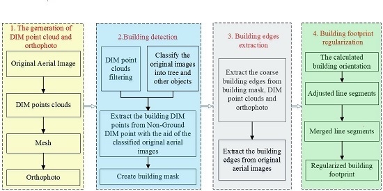
Our proposed approach for building detection and boundary regularization consists of four stages: (1) The generation of DIM point clouds and orthophoto from original aerial images; (2) individual building detection from DIM point clouds with the aid of original aerial images; (3) building edge detection using a feature-level fusion strategy; and (4) regularization of building boundaries by the fusion of matched lines and boundary lines. The entire workflow is shown in Figure 2.
2.1. Generation of DIM Point Clouds and Orthophoto from Original Aerial Images
Our proposed method takes the aerial images as an input. The features from aerial images and DIM points will be employed in the process of detecting buildings and the straight-line features from orthophoto will be used to help building edge detection. Therefore, the generation of DIM point clouds and true orthophoto from original aerial images is the top priority of our proposed method.
In this paper, we applied the commercial package Agisoft PhotoScan [42] which is able to automatically orient and match large datasets of images to generate the DIM point clouds and orthophoto. Due to commercial considerations, little information is available concerning the internal algorithms employed. Hence, we will describe the process of the generation of the DIM point clouds and orthophoto based on the workflow of Agisoft PhotoScan. Specially,
- Add the original images, the positioning and orientation system (POS) data and the camera calibration parameters into this software.
- Align photos. In this step, the point features are detected and matched; and the accuracy camera locations of each aerial image are estimated.
- Build the dense points clouds. According to a previous report [21], a stereo semi-global matching like (SGM-like) method is used to generate the DIM point clouds.
- Make use of the DIM points to generate a mesh. In nature, the mesh is the DSM of the survey area.
- Build the orthophoto using the generated mesh and the original aerial images.
Figure 3a,b shows the generated orthophoto and the DIM point clouds of the test area 3 of the Vaihingen dataset.
2.2. Building Detection from DIM Point Clouds with the Aid of the Original Aerial Image
2.2.1. Filtering of DIM Point Clouds
Filtering of the point clouds is the process of separation of ground points from the non-ground points and is the first step to detect buildings. Multiple filtering methods [43,44] have been proposed. Among these methods, the progressive triangular irregular network (TIN) densification (PTD) algorithm [45] is one of the most popular algorithms in engineering applications. However, this method may fail to extract the ground points because the density and the noise of DIM point clouds are higher than that of the ALS point cloud. Hence, an improved PTD algorithm [46] is selected
The improved PTD is divided into two steps. The first step is selecting seed points and constructing the initial TIN. The second step is an iterative densification of the TIN. The largest differences between the PTD and the improved PTD is the procedure for calculating densification thresholds. In the improved PTD, the angle threshold changes from high to low, and with the increase of the density of points added into the TIN, the angle threshold becomes large. Using this method, we can remove the ground points and low objectives points. The remaining points only contain building and tree points.
2.2.2. Object-Oriented Classification of Original Aerial Images
Generally, it is easier to detect trees from aerial images than to detect buildings. Based on this, we classify the aerial images into two categories: trees and other objects. Here, the commercial classification software eCognition 9.0.2 is used to detect trees from each aerial images. In this section, the original aerial images are classified, so that the classification results of each original aerial image can be employed in the later stage. The process of object-oriented classification is divided into three steps:
- Multi-resolution segmentation of the aerial image. This technique is used to extract reasonable image objects. In the segmentation stage, several parameters, such as layer weight, compactness, shape, and scale, must be determined in advance. These algorithms and related parameters are described in detail in [47]. Generally, the parameters were determined through visual assessment as well as trial and error. We set the scale factor as 90 and set the weights for red, green, blue and straight-line layers are 1, 1, 1, and 2, respectively. The shape and compactness parameters are 0.3 and 0.7, respectively.
- Feature selection. The normalized difference vegetation index (NDVI) has been used extensively to detect vegetation [48]. However, relying on the NDVI alone to detect the vegetation is not accurate due to influence of shadows and colored buildings on aerial images [16]. Therefore, besides the NDVI, the texture information in the form of entropy [49] is also used on the basis of the observation that trees are rich in texture and have higher surface roughness than building roofs [16]. Moreover, R, G, B, and brightness are also selected as the features in our proposed method. Notably, if the near-infrared band is not available, color vegetation indices can be calculated from color aerial images. In this paper, we applied the green leaf index (GLI) [50,51] to replace NDVI. The formula of the GLI is expressed in the formula (1). In this formula, R, G and B represents the value of the red, green and blue bands of each pixel from original aerial image, respectively.
- Supervised classification of segments using a Random Forest (RF) [52]. The reference labels are created by an operator. The computed feature vector per segment is fed into the RF learning scheme. To monitor the quality of learning, the training and prediction is performed several times.
2.2.3. Removal of Tree Points from Non-Ground DIM Points
In this stage, the tree DIM points will be removed from non-ground DIM points with the aid of the classified original aerial images. The process of removing tree points from non-ground DIM points is described as follows:
- At first, define a vector L. The size of L is equal to the number of non-ground DIM points and each element within this vector is used to mark the category of each corresponding non-ground DIM point. In the initial stage of this process, we set the value of each element within this vector to 0, which indicates that the corresponding DIM point is unclassified.
- Then, select a classified original aerial image and make use of this classified original aerial image to label the category of each element within the vector L. The fundamental of this step is back projection. If the calculated projected point of a non-ground DIM point falls within the region which is labelled as tree in the selected image, the corresponding element within L plus 1; otherwise, the corresponding element within L minus 1.
- Continue the second step until all classified original aerial images are traversed.
- If the value of an element within the vector L is greater than 0, the corresponding non-ground DIM point is regarded as a tree point; otherwise, the DIM point is a building point.
In the second step of the above process, the visibility analysis and occlusion detection is necessary during the back projection. The purpose of visibility analysis is to determine whether the selected DIM point is within the selected image’s field of view (FOV) and face the image’s direction without occlusion from other objects. In this paper, we make use of the collinear equations and an image’s interior/exterior orientation parameters to determine whether the selected DIM point is within an image FOV and applied the method in [53] for occlusion detection. If a non-ground DIM point is invisible or occluded in the selected classified original aerial image, the value of the corresponding element within L remains unchanged.
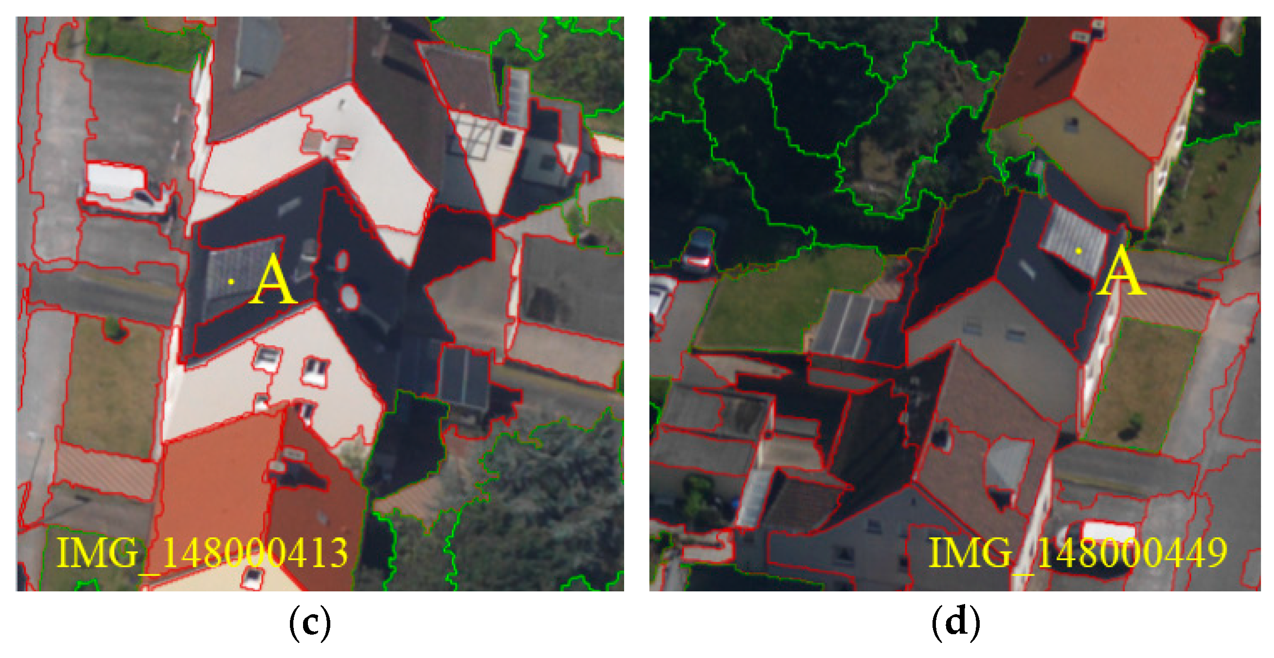
Here, we take a DIM point as an example to further describe the process of removing tree points from non-ground DIM points. As is shown in Figure 4, the projected point of the selected DIM point is marked as and is invisible at the viewpoint of image IMG_147000509. Therefore, the value of the corresponding element within L remains unchanged when the image IMG_147000509 is applied in this process. In image IMG_147000345, due to the impact of illumination and texture, the region where the projected point falls is incorrectly divided into the tree category. Based on the description of the above process, the value of the corresponding element plus 1. In the image IMG_147000413 and IMG_147000449, the projected point falls in the region marked as other objects. Hence, the value of the corresponding element within the vector L minus 1, respectively. After 4 images are traversed, the corresponding element value is less than 0. Obviously, the DIM point will be regarded as a building point.
The classification results are shown in Figure 5b. Figure 5c,d show the advantages of our proposed method. The low building marked as in Figure 5c is occluded at the nadir viewpoint, which results in this building remaining undetected from the orthophoto. However, in our proposed method, this low building can be detected from DIM points as is shown in Figure 5d.
2.2.4. Extraction of Individual Building from the DIM Points
Some scattered points remain distributed in 3D space because of the wrong category of DIM points. To remove these interference points, the octree method is used to divide the point cloud into 3D grids. If the number of the DIM points in a user-defined 3D grid is beyond a certain threshold, the grid is preserved. This threshold is determined by the size of the grid and the density of the DIM points. Generally speaking, the smaller the grid size is, the smaller this threshold is; and the higher the density is, the larger the threshold is.
Project the 3D points onto the planar coordinates with the resolution of the orthophoto; and a morphological close operator with a square structuring element is used to generate an initial binary image. This structuring element is estimated by the density of DIM points and the resolution of planar coordinates. Then, a two-pass algorithm [54] is used to extract the connected components. Each connected component represents an individual building blob.
2.3. Building Edge Detection Using a Feature-Level Fusion Strategy
The boundaries of individual buildings obtained in Section 2.2 are irregular. In this section, the straight-line segments are extracted from the DIM points, orthophoto and building blob. Subsequently, the coarse building edges from the DIM points, orthophoto, building mask, and height information from DIM points are fused to help match extracted straight-line segments from aerial images so that the matched line segments can be used for regularization of building boundaries.
2.3.1. Detection of Coarse Building Edges from the DIM Points, Orthophoto and Building Mask
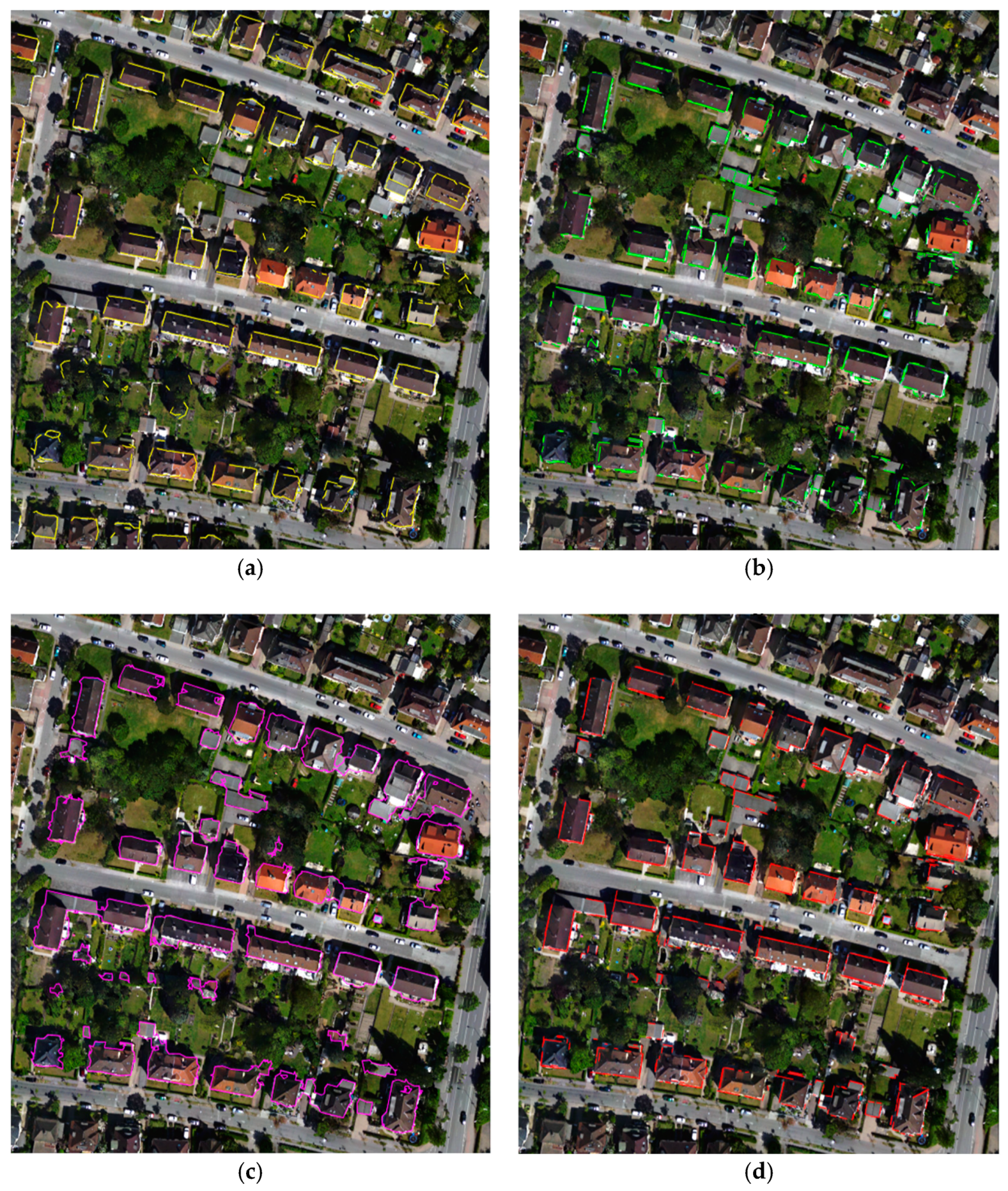
In this section, three kinds of building edges are extracted: the building edges from DIM points, the building edges from orthophoto and the building edges from extracted building blob. Figure 6a–c shows the extracted results of the three kinds of building edges. All these building edges are mainly used to assist the straight-line segments from original aerial images to match in the later stage. The process of detecting the three kinds of building edges is described as follows:
- Detection of building edges from DIM points. In terms of DIM point clouds, the building facades are the building edges. Hence, how to extract the building edges from DIM points is converted to how to detect the building facades from DIM points. The density of DIM points at the building façades is larger than that at other locations. Based on this, a method [55] named as the density of projected points (DoPP) is used to obtain the building façades. If the number of the points located in a grid cell is beyond the threshold thr, the grid is labelled 255. After these steps, the generated façade outlines still have a width of 2–3 pixels. Subsequently, a skeletonization algorithm [56] is performed to thin the façade outlines. Finally, a straight-line detector based on the freeman chain code [57] is used to generate building edges.
- Detection of building edges from orthophoto. The process of extracting building edges from orthophoto is divided into three steps. First, a straight-line segment detector [58] is used to extract straight-line segments from the orthophoto. Second, a buffer region is defined by a specified individual building blob obtained in Section 2.2. If the extracted straight-line segment intersects the buffer region, this straight-line segment is considered as a building candidate edge. Finally, the candidate edge is discretized into t points. The number of points located in buffer region is i. represents the length of the candidate edge falling into the buffer area. The larger this ratio is, the greater the probability that this candidate edge is the building edge is. In this paper, if this ratio is greater than 0.6, the candidate edge is considered a building edge.
- Detection of building edges from the building blob. The boundaries of buildings are estimated using the Moore Neighborhood Tracing algorithm [59], which provides an organized list of points for an object in a binary image. To convert the raster images of individual buildings into a vector, the Douglas-Peucker algorithm [60] is used to generate the building edges.
2.3.2. Detection of the Building Boundary Line Segments from the Original Aerial Images by Matching Line Segments
In this section, the basic process unit is an individual building. Before the line matching, both the straight-line segments from original aerial images and the DIM points of the selected individual building are obtained; then, the height information from DIM points is used to obtain an alternative matching line pool of a selected coarse building edge; finally, a line matching algorithm based on the three-vision images is applied to obtain the matched building edges from the alternative matching line pool. Specifically,
- Obtain the associated straight-line segments from multiple original aerial images and DIM points of an individual building
- ■
- Select an individual building detected in Section 2.2.4.
- ■
- According to the planar coordinate values of the individual building, obtain the corresponding DIM points.
- ■
- Project the DIM points onto the original aerial images, and obtain the corresponding regions of interest (ROIs) of selected individual building from multiple aerial images. Employ the straight-line segments detector [58] to extract the straight-line segments from corresponding ROIs. The extracted straight-line segments from ROIs are shown in Figure 7.
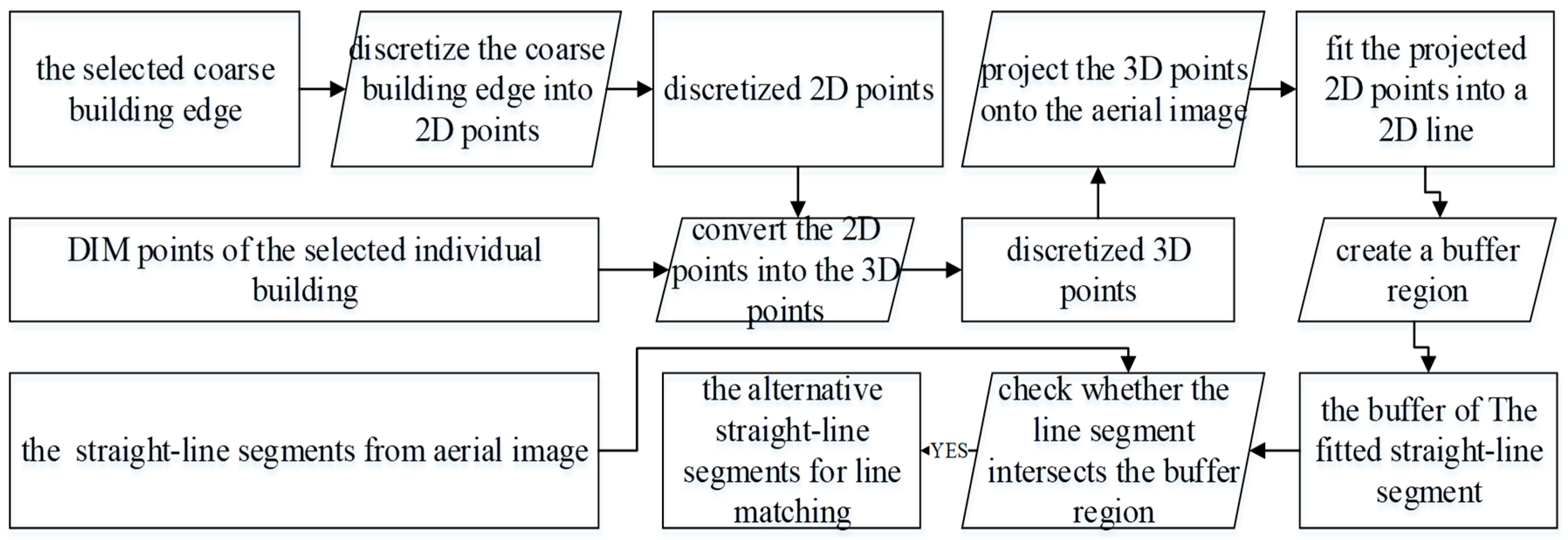
• The generation of an alternative matching straight-line segments pool of a coarse building edge
Figure 8 shows the process of the generation of alternative matching straight-line segments of a coarse building edge. We divide the process into three steps; and the details are described as follows.
- ■
- Choose a coarse building edge, and discretize this straight-line segment into 2D points according to the given interval . Use the nearest neighbor interpolation algorithm [61] to convert the discretized 2D points into 3D points by fusing the height information from the DIM points. Notably, the points at the building facades which have been detected by the method DoPP should be removed before interpolation so that we can obtain the exact coordinate values of each 3D point.
- ■
- Project the 3D points onto the selected original image according to the collinear equation. In this step, occlusion detection is necessary.
- ■
- Fit the projected 2D points into a straight-line segment on the selected aerial image. A buffer region with the given size is created. Check whether the associated line segments from aerial image intersect the buffer region. If a straight-line segment from aerial image intersects within the buffer, the line is labelled as an alternative line.
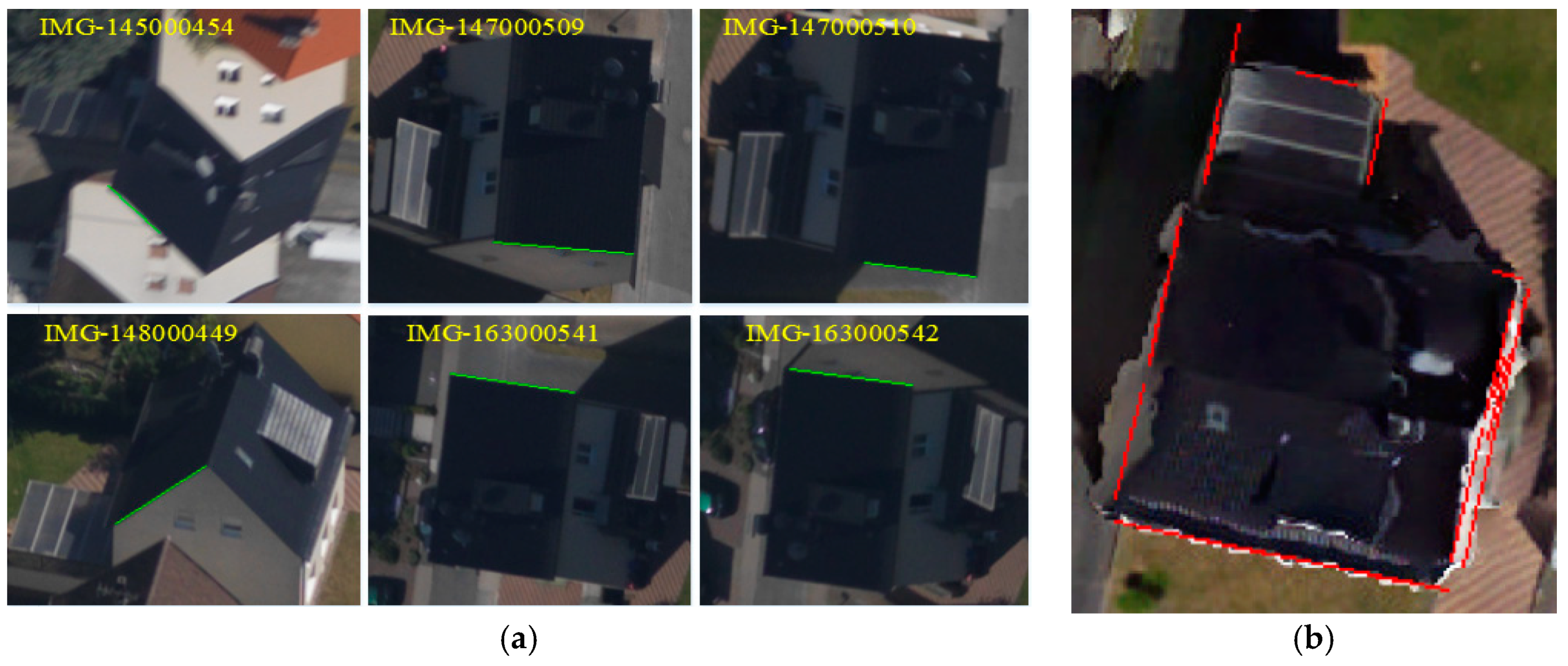
The number of line segments that intersect the buffer may be more than one in an image. To reduce the complexity of line matching, only the longest line is selected. After all the associated images are processed, an alternative matching line pool of the selected coarse building edge is created. Figure 9 shows the generated alternative matching line pool. In Figure 9, the IMG-n represents the image in the generated alternative matching line pool and the red line is the selected alternative matching line.
• Straight-line segments matching based on three-vision images
After the generation of alternative matching straight-line segments pool of a selected coarse building edge, the straight-line segments matching process starts.
- ■
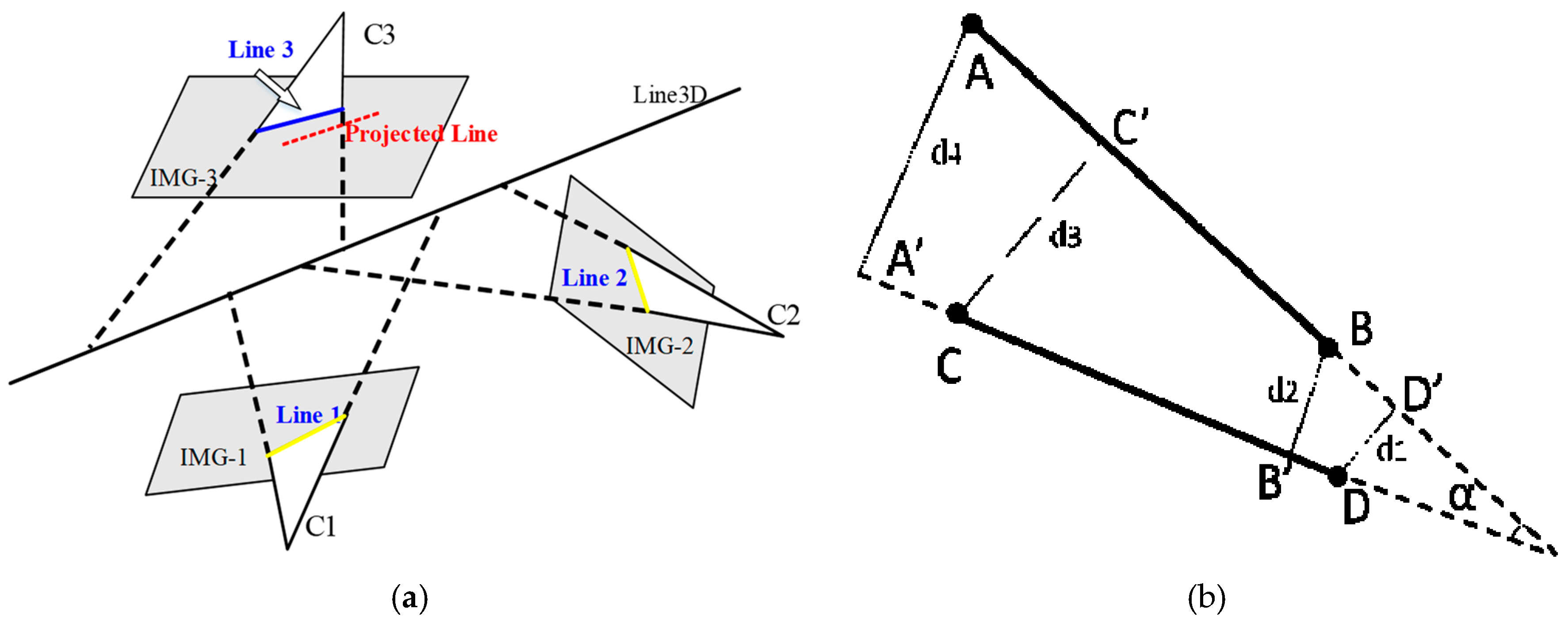
- Select two longest line segments from the alternative matching line pool. As is shown in Figure 10a, it is obvious that the camera is not on the straight-line segment Line 1. Similarly, both the camera and are not on the straight-line segment and , respectively. Hence, a 3D plane is generated by the camera and the straight-line segment . Another plane is created by camera and the line segment . Two planes intersect into a 3D line segment.
- ■
- Project the 3D line segment onto the IMG-3. If the projected line and overlap each other, calculate the angle and normal distance between and the projected line; otherwise, return to the first step. In the process, the occlusion detection is necessary. The normal distance is expressed as Equation (2), and are shown in Figure 10b.
If the angle is less than and the normal distance is less than , the three straight-line segments can be regarded as homonymous lines; otherwise, return to the first step.
- ■
- To ensure the robustness and accuracy of line matching, the three homonymous lines should be checked. In accordance with the method described in the previous step, use the camera 1 and the line segment to generate a 3D plane, and use the camera 3 and the line segment to generate another 3D plane. Two planes intersect into a 3D line. Project the 3D line onto IMG-2. Check whether the normal distance and the angle between Line 2 and the projected line satisfy the given thresholds. Similarly, check the normal distance and angle between and the projected line, which is generated from and . If the normal distance and angle still satisfy the given thresholds, the three lines can be considered homonymous lines; otherwise, return to the first step.
- ■
- Make use of the three homonymous lines to create a 3D line. Project the 3D line onto the other aerial images. According to the given thresholds, search the homonymous line segments. The results are shown in Figure 11a. Make use of the homonymous lines to create a 3D line, and project the 3D line onto the plane. A new building edge can be created.
• Iterate the second and third steps until all the coarse building edges are processed. The matched lines of the selected individual building are shown in Figure 11b.
2.4. Regularization of Building Boundaries by the Fusion of Matched Lines and Boundary Lines
In this section, the matched straight-line segments from original aerial images and the straight-line segments from building blob are fused to generate the building footprint. First, the boundary line is adjusted to the specified angle. Then, the parallel line segments are merged. Finally, a new method for building boundary regularization is proposed.
2.4.1. Adjustment of Straight-Line Segments
Buildings typically have one or more principal directions. The direction of the true building edge should be in consonance with the building’s direction. Under this principle, the lines should be adjusted to the building’s main direction. The matched straight-line segments from original aerial images can be used to calculate the building’s direction. The selected straight-line segments are divided into nine intervals according to the line angles. Given that there are lines in an interval, the total length of n straight-line segments can be calculated and labelled as i. A histogram is generated using i. The peak of the histogram represents the building’s direction. The equation can be expressed as follows.
Buildings are diverse; some buildings have complex structures and contain relatively more directions. If the total value of an interval is more than 0.3 times the maximum value, the angle value can be regarded as another direction of the building. After the estimation of the dominant directions, the lines from the blob of individual buildings are adjusted slightly according to the dominant directions of buildings. The line adjustment process can be described as follows. First, a line is selected, and the adjustment angle is calculated; then, the line is rotated around the midpoint of the processing line. The adjustment results are shown in Figure 12a.
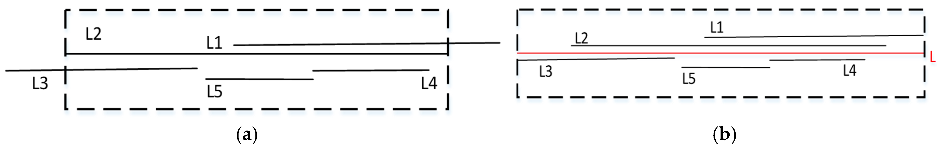
2.4.2. Merging of Straight-Line Segments
Figure 13 shows the process of five parallel line segments that are merged to one average line segment. First, the longest line segment is selected, and a buffer area is created by a given threshold of as shown in Figure 13a. Then, each line segment is checked for parallelism to . If a line is parallel to and intersects the buffer area, the line is added to the line segments set m. When all line segments are processed, line segments , , and are selected. Given that the equation of the straight-line i is i, we conclude that the length of the line segment in m affects the location of the merged line. A longer line segment corresponds to a greater weight. The equation of the merged straight-line is expressed as follows.
In this equation , and represents the length of the line segment . To obtain the merged line segment, the endpoint of each line segment is projected to the generated straight-line segments. All the projected points are added to the point set . The longest line segment within two projected points is the merged line segment as shown in Figure 13b. The results of merged lines are shown in Figure 12b.
2.4.3. Building Footprint Generation
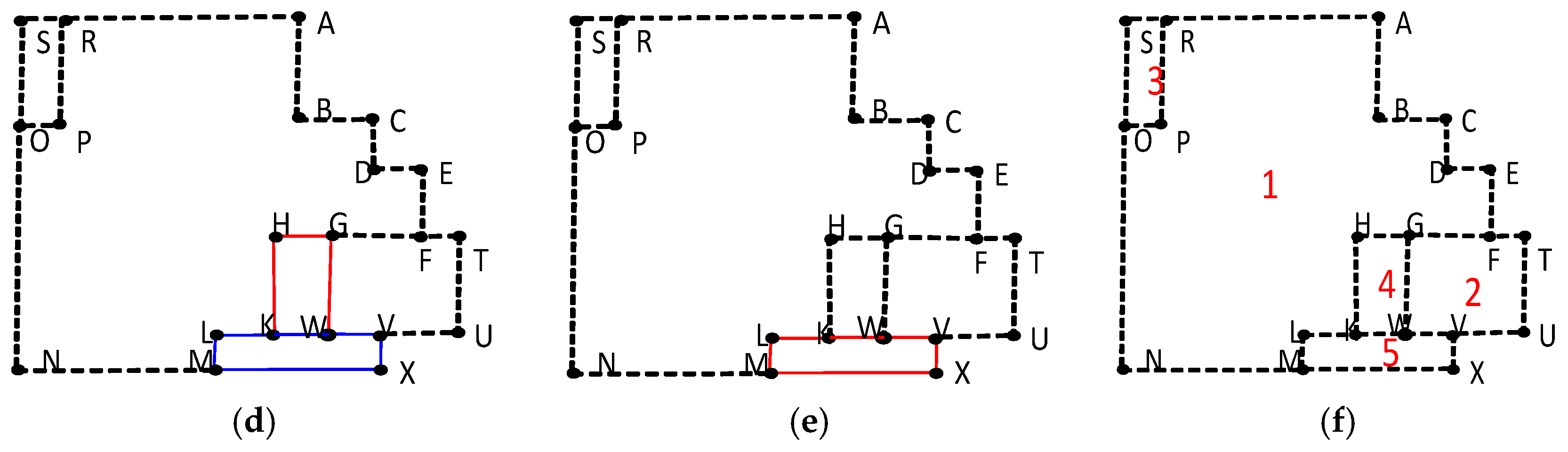
Gaps exist between the two merged line segments. To obtain a complete building profile, these gaps should be filled. As shown in Figure 12c, point B is an endpoint of the line segment and a gap exists between line segment AB and the line segment CD. To fill this gap, a new strategy is proposed.
- First, calculate the distances from the point B to the other line segments in three directions—along the direction and two vertical directions of line segment AB. As shown in Figure 12c, the distance from the point B to the line segment CD is BK; the distance from the point B to the line segment EF is BM + ME; and the distance from the point B to the line segment HG is BN + NG.
- Search the minimum distance among the calculated distances from the point B to the other line segments. The line segment BK is the gap between the line segment AB and CD.
- Continue the above two steps until all the gaps are filled. The results are shown in Figure 12d.
After the gaps are filled, the invalid polygons that contain a small amount of areas of the detected building mask, such as the rectangle EFIJ in Figure 12d, should be removed. Before the process, we need to search from the non-overlapping single polygon from the entire polygons. Figure 14 shows the process of searching the non-overlapping single polygon.
- First, the endpoints are coded again, and the line segments are labelled. If the line segment is located on the external contour of the entire polygon, the straight-line segment is labelled as 1; otherwise, the line segment is labelled as 2, as shown in Figure 14a.
- Choose a line arbitrarily from the lines dataset as the starting edge. Here, the line segment is selected.
- Search the line segments that share the same endpoint . If only a straight-line segment is searched, then the line segment is the next line segment. If two or more straight-line segments are found, calculate the angle clockwise between each alternative line segment and this line segment EF. The angle between the line and is , and the angle between the line and is 90°. Choose the straight-line segment as the target line segment based on the smaller calculated angle value.
- Search until all the straight-line segments are removed. The result is shown in Figure 14f.
Within each preserved polygon, the total number of pixels is , and the number of pixels present in the building is . If the is larger than the given threshold , the polygon is preserved; otherwise, the polygon is removed. The preserved polygon is shown in Figure 12e. Merge the preserved single polygon; the outline of the merged polygon is the building footprint, as shown in Figure 12f.
3. Experiments and Performance Evaluation
3.1. Data Description and Study Area
The performance of the proposed approach is tested on three datasets: Vaihingen (VH), Potsdam and Lunen (LN). The VH dataset consists of vertical aerial images; the Potsdam and LN datasets are composed of oblique aerial images. These datasets have different complexities and surrounding conditions. Each dataset is listed as follows:
- VH. The VH dataset is published by the International Society for Photogrammetry and Remote Sensing (ISPRS), and has the real ground reference value. The object coordinate system of this dataset is the system of the Land Survey of the German federal state of Baden Württemberg, based on a Transverse Mercator projection. There are three test areas in this dataset and have been presented in Figure 15a–c. The orientation parameters are used to produce DIM points, and the derived DIM points of three areas have almost the same point density of approximately 30 2.
- ■
- VH 1. This test area is situated in the center of the city of Vaihingen. It is characterized by dense development consisting of historic buildings having rather complex shapes, but also has some trees. There are 37 buildings in this area and the buildings are located on the hillsides.
- ■
- VH 2. This area is flat and is characterized by a few high-rising residential buildings that are surrounded by trees. 14 buildings are in this test area.
- ■
- VH 3. This is a purely residential area with small detached houses and contain 56 buildings. The surface morphology of this area is relatively flat.
- Potsdam. The dataset including 210 images was collected by TrimbleAOS on 5 May 2008 in Potsdam, Germany and has a GSD of about . The reference coordinate system of this dataset is the WGS84 coordinate system with UTM zone 33N. Figure 15d shows the selected test area, which contains 4 patches according to the website (http://www2.isprs.org/commissions/comm3/wg4/2d-sem-label-potsdam.html): 6_11, 6_12, 7_11 and 7_12. The selected test area contains 54 buildings and is characterized by a typical historic city with large building blocks, narrow streets and a dense settlement structure. Because the collection times between the ISPRS VH benchmark dataset and the Potsdam dataset differ, the reference data are slightly modified by an operator.
- LN. This dataset including 170 images was collected by the Quattro DigiCAM Oblique system on 1 May 2011 in Lunen, Germany and has a GSD of . The object coordinate system of this dataset is the European Terrestrial Reference System 1989. Three patches with flat surface morphology were selected as the test areas. The reference data are obtained by a trained operator. Figure 15e–f shows the selected areas.
- ■
- LN 1. This is a purely residential area. In this area, there are 57 buildings and some vegetation.
- ■
- LN 2. In this area, there are 36 buildings and several of these buildings are the occluded by tress.
- ■
- LN 3. This area is characterized by a few high-rising buildings with complex structures. In this area, 47 buildings exist.
3.2. Evaluation Criterion
The evaluation index system adopted by ISPRS [62] is applied for a quality assessment of our proposed approach. In this evaluation system, three categories of evaluations are performed: object-based, pixel-based, and geometric, where each category uses several metrics. The object-based metrics (completeness, accuracy, quality, under- and over-segmentation errors, and reference cross-lap rates) evaluate the performance by counting the number of buildings, while the pixel-based metrics (completeness, accuracy, quality, area-omission, and area-commission errors) measure the detection accuracy by counting the number of pixels. The geometric metric (root mean square error, i.e., RMSE) indicates the planimetric distance in meters accuracy from extracted outlines to a reference outline. The RMSE, correctness, completeness, and quality equations are shown in Equations (5).
where represents the number of points for which a correspondence has been found within a predefined search buffer, is the distance between the corresponding points, represents the number of true positives, represents the number of false positives, and represents the number of false negatives. In the evaluation process of our proposed approach, the building area is taken into consideration. The minimum areas for large and small buildings are set to 50 2 and 2.5 2, respectively. The symbols used in the assessment are described in Table 1.
3.3. Results and Discussion
Section 3.3.1 and Section 3.3.2 describe and discuss the evaluation results of our proposed technique on the VH, Potsdam and LN datasets.
3.3.1. Vaihingen Results
Table 2 and Table 3 show the official per-object and per-area level evaluation results for the three test areas of the VH dataset. Figure 16 shows the per-pixel level visual evaluation of all the test areas (column 1) for the building delineation technique (column 3) and their corresponding regularization outcome (column 2).
Table 2 shows that the overall object-based completeness and accuracy are 83.83% and 98.41%, respectively; the buildings over 2 are extracted with objective completeness and accuracy before regularization. The missing buildings (marked “green circle” in Figure 16a,d,g) are eliminated in the process of building detection. Building detection consists of two steps: DIM point clouds filtering and object-oriented classification of original aerial images. Figure 17 shows the results of DIM point cloud filtering on the VH dataset. Only two small buildings (marked “green circle” in Figure 17a,c) are removed due to the improper filtering thresholds. Most of the missing buildings (marked “yellow circle” in Figure 17a–c) are removed in the process of object-oriented classification of original aerial images, which indicates that the errors of building detection mainly occur at this stage. To increase the detection rate, the accuracy of object-oriented classification of original aerial images should be improved.
Certain close buildings were combined unexpectedly (marked as , and ), as shown in Figure 16i because the quality of DIM point clouds is lower than that of LiDAR point clouds, particularly in the regions between two buildings. In addition to the many-to-1 () segmentation errors, many-to-many () segmentation errors marked as in Figure 15b exist. These many-to-many () segmentation errors are caused by two factors. On the one hand, the filter threshold removes the low part of the building, as shown in Figure 16a, and the buildings are segmented into several parts; on the other hand, a building and a segmented part are merged into a building at the same time. Moreover, there are two incorrectly detected buildings (objects under a tree and shuttle bus), as shown in Figure 16h marked as . After regularization, the object-based results are the same as those before regularization.
After regularization, the per-area completeness, accuracy, and quality are improved. The pixel-based completeness and accuracy are and , respectively. This increase might be substantial if the straight-line segments from the DIM points, orthophoto and original images could replace the line segments from the boundary of the detected building mask. After the boundary is regularized efficiently, the planimetric accuracy is improved from to .
3.3.2. Potsdam and LN Results
Table 4 and Table 5 present the object- and pixel-based evaluation of the detection technique before and after the regularization. Figure 18 and Figure 19 show the extracted buildings and their corresponding building footprints for Potsdam, and . The proposed building detection method extracted 49, 52, 35, and 39 buildings out of 54, 57, 36, and 47 reference buildings in the Potsdam, , and , respectively.
The object-based completeness and accuracy on all the buildings are and respectively, as shown in Table 4. A building over 2 marked as in Figure 18d is missed due to the influence of shadows in the process of tree removal. Table 5 shows the total per-area evaluation (completeness and accuracy and , respectively) of the proposed building detection method for Potsdam and Lunen before regularization. The per-area completeness in is lower than that of the three remaining areas (Potsdam, and ), mainly because the roof of the buildings is not detected completely because of the misclassification of the tree and building, as shown in Figure 19f. Moreover, there are some sundries surround the building; these objects are regarded as the parts of the true building, which causes the per-area accuracy in to be lower () than that in the other three areas. Figure 18j shows this example. The average pixel-based completeness and accuracy increase significantly from and to and after the regularization, respectively. Similarly, three factors hinder the detection of buildings in the process of building detection.
- Initially, the filtering threshold may be larger than the height of low buildings. In our test arrangement, some low buildings () are excluded in the filtering process. Fortunately, the height of most buildings is higher than the given thresholds in the Potsdam and Lunen test areas. Only the building marked as in Figure 18b is removed.
- Second, the misclassification of trees and other objects in the process of object-oriented classification of original aerial images is the main reason that affects the accuracy of building detection. Some buildings are removed due to the influence of similar spectral features and shadow. Figure 18f,g,i and Figure 19h,i shows examples of missed buildings. Similarly, some trees are classified as buildings, as shown in Figure 18f.
- Third, the noise of DIM points degrades the accuracy of building detection. Uncoupled to the over-segmentation error, under- and many-to-many segmentation errors exist in Table 4. Figure 19g shows the many-to-many segmentation error example. The shadow on the surface of the building leads to the over-segmentation of the building, and the adjacent buildings are combined with the building at the same time due to the small connecting regions between these two buildings.
3.4. Comparative Analysis
In our proposed method (PM), we solely employed aerial images as the data source to extract buildings in complex urban scenes. To compare our proposed method with other methods, we select those which use aerial images alone and the supervised classification strategy. According to the ISPRS portal and the classified methods in [8], three methods—DLR, RAM and Hand—are selected for the comparative analysis. In addition, we hope that our proposed method is superior to other methods combining the images and LiDAR data. Hence, in addition to these three methods just mentioned, Fed_2, ITCR and MON4 are also chosen. In Fed_2, LiDAR data are used to detect buildings, and the footprint of buildings are generated by the straight-line segment from the orthoimagery. In ITCR, the LiDAR data and the original images are fused, and a supervisory strategy is used for building detection. MON4 make use of a method named as Gradient-based Building Extraction (GBE) to extract the building planes and their neighboring ground planes from images and Lidar; then, analyzes the height difference and connectivity between the extracted building planes and their neighboring ground planes to extract low buildings. These chosen methods can be seen in Table 6.
Table 7 presents a comparison between our proposed method and six other methods. From the comparison results of the different methods in the VH dataset, several conclusions can be obtained as follows:
- Relative to RMA and Hand, our proposed method can obtain similar object-based completeness and accuracy in VH1 and VH3. The object-based accuracy of RMA and Hand in is 52% and 78%, respectively, and is significantly lower than that of the proposed method because NDVI is the main feature in RMA and Hand. The wrong NDVI estimate decreases the object-based accuracy in VH2 due to the influence of shadow pixels. The results show that our proposed method is more robust than RMA and Hand due to the use of additional features.
- The DLR not only divides the objects into buildings and vegetation but also takes into account vegetation shadowed in the separation of buildings and other objects. Therefore, the pixel-based completeness and accuracy of DLR is slightly higher than that of our proposed method in VH1, VH2 and VH3. Moreover, the pixel-based completeness and accuracy of DLR is also higher than that of other 4 methods. The object-based completeness of DLR is lower than that of our proposed method in VH2 and VH3, mainly because the features from original aerial images are used to detect buildings and because the small buildings can be easily detected in the two areas. Actually, there are seldom buildings that are occluded in the three test areas of Vaihingen. The advantages of our proposed method are not thoroughly demonstrated. The buildings labelled as k in Figure 18d and Figure 19e are partially or completely occluded, and DLR cannot detect the occluded buildings. In our proposed method, the occluded building can be detected. Notably, because the noise of DIM points is higher than that of LiDAR point cloud, the object-based accuracy of the proposed method is slightly lower than that of DLR in VH3. Large buildings (50 2) were extracted with 100% accuracy and completeness.
- The proposed method offers better in object-based completeness and accuracy than ITCR, mainly because the LiDAR point clouds need to be segmented into 3D segments that are regarded as the processed unit in ITCR. The process produces segmented errors that damage the building detection results. Furthermore, the segmentation of DIM points is more challenges because the quality of DIM points is lower than that of the LiDAR point cloud. Therefore, we make use of the aerial images to detect buildings from non-ground points to replace the segmentations of the DIM point cloud in our proposed method.
- Fed_2 and our proposed method obtain better performance than ITCR and IIST because the segmented errors are avoided in the process of building detection. The performance of Fed_2, MON4 and our proposed method is approximately the same.
The above analysis shows that our proposed algorithm is robust and can obtain similar performance of building detection methods that fuse LiDAR data and images. Moreover, the RMSE is decreased due to the boundary lines being replaced with the matched lines from the original aerial images.
3.5. Performances of Our Proposed Building Regularization
Section 3.4 shows that the directions of buildings are the precondition for the building regularization. To evaluate the performance of the regularization technique, we divide the buildings into three categories: single-direction buildings, multi-direction buildings and complex structure buildings. The regularization results of single-direction buildings and multi-direction buildings are shown in Figure 20a–n.
In our proposed method, the matched lines are used in the process of searching the direction of building. According to the line segments from the mask of the detected buildings, the usage of adjusted lines increases the . Figure 20a–f,k–l shows relevant examples. Nevertheless, incorrectly adjusted line segments remain, particularly involving the multi-direction buildings, as shown in Figure 20g–j,m,n, mainly because building’s directions cannot be computed completely due to the absence of line segments that provide the directions of buildings. As shown in Figure 20g–j,m–p, these buildings have two directions. However, only one direction is calculated correctly; the other direction is ignored in the examples. As a result, some lines deviate from the true direction.
In terms of the complex structure building, holes exist. To obtain the accurate footprint, both the external contours and inner contours from the mask of detected building are calculated, respectively. According to the contours, we group the lines and regularize the contours. These regular contours construct the footprint of the complex structure building. Figure 20o,p shows the examples of this building. Notably, if the size of the hole is smaller than the given thresholds, we can ignore the inner contour.
4. Conclusions
This paper focuses on both building detection and footprint regularization using solely aerial images. A framework for building detection and footprint regularization using a feature-level-fusion strategy is proposed. Following a comparison with six other methods, the experiment results show that the proposed method can not only provide comparable results to building detection methods using LiDAR and aerial images but also generate building footprints in complex environments. However, several limitations for our proposed method cannot be ignored:
- In the building detection stage, the results of building detection rely on the results of object-oriented classification of original aerial images. Shadows are an important factor influencing the classification of original aerial images. In the process of classification, we categorize the objects into only two classes (trees and other objects) and do not train and classify shadows as separate objects. As a result, the classification results cannot perform perfectly. In the further work, we will make use of the intensity and chromatic to detect the shadow so that we can get better performance.
- The noise of the DIM point cloud produced by dense matching is higher than that of the LiDAR point clouds. The buildings detection results and footprint regularization are affected by noise.
- A threshold exists in the process of DIM point cloud filtering. The filtering threshold cannot ensure that all the buildings can be preserved. In fact, the low buildings may be removed, while some objects that are higher than the threshold are preserved. The improper threshold causes detection errors.
- At the stage of building footprint regularization, only straight lines are used. Therefore, for a building with a circular boundary, our proposed method cannot provide satisfactory performance.
- Finally, the morphology of buildings also influences the accuracy of building detection results. In fact, the more complex the building morphology is, the more difficult the building boundary regularization is.
Author Contributions
Y.D. has developed, implemented and conducted the tests. In addition, he has written the paper. L.Z. and X.C. wrote part of the manuscript, and performed the experiments and experimental analysis. H.A. proposed the original idea. B.X. made the contribution on the programming, and revised the manuscript.
Funding
This research was funded: (1) National Natural Science Foundation of China, grant number 51474217; (2) National Key Research and Development Program of China, grant number 2017YFB0503004; (3) the Basic Research Fund of Chinese Academy of Surveying and Mapping, grant number 7771801, respectively.
Acknowledgments
The authors would like to thank the anonymous reviewers for their constructive comments, which greatly improved the quality of our manuscript. The Vaihingen data set was provided by the German Society for Photogrammetry, Remote Sensing and Geoinformation (DGPF). The Lunen data set was provided by Integrated Geospatial Innovations (IGI). The Potsdam data set was provided by Trimble. Moreover, we thank X.L. for revising the language.
Conflicts of Interest
The authors declare no conflict of interest.
References
- Krüger, A.; Kolbe, T.H. Building Analysis for Urban Energy Planning Using Key Indicators on Virtual 3d City Models—The Energy Atlas of Berlin. ISPRS Int. Arch. Photogramm. Remote Sens. Spat. Inf. Sci. 2012, XXXIX-B2, 145–150. [Google Scholar]
- Arinah, R.; Yunos, M.Y.; Mydin, M.O.; Isa, N.K.; Ariffin, N.F.; Ismail, N.A. Building the Safe City Planning Concept: An Analysis of Preceding Studies. J. Teknol. 2015, 75, 95–100. [Google Scholar]
- Murtiyoso, A.; Remondino, F.; Rupnik, E.; Nex, F.; Grussenmeyer, P. Oblique Aerial Photography Tool for Building Inspection and Damage Assessment. ISPRS Int. Arch. Photogramm. Remote Sens. Spat. Inf. Sci. 2014, XL-1, 309–313. [Google Scholar] [CrossRef]
- Vetrivel, A.; Gerke, M.; Kerle, N.; Vosselman, G. Identification of damage in buildings based on gaps in 3D point clouds from very high resolution oblique airborne images. ISPRS J. Photogramm. Remote Sens. 2015, 105, 61–78. [Google Scholar] [CrossRef]
- Karimzadeh, S.; Mastuoka, M. Building Damage Assessment Using Multisensor Dual-Polarized Synthetic Aperture Radar Data for the 2016 M 6.2 Amatrice Earthquake, Italy. Remote Sens. 2017, 9, 330. [Google Scholar] [CrossRef]
- Stefanov, W.L.; Ramsey, M.S.; Christensen, P.R. Monitoring urban land cover change: An expert system approach to land cover classification of semiarid to arid urban centers. Remote Sens. Environ. 2001, 77, 173–185. [Google Scholar] [CrossRef]
- Antonarakis, A.S.; Richards, K.S.; Brasington, J. Object-based land cover classification using airborne LiDAR. Remote Sens. Environ. 2008, 112, 2988–2998. [Google Scholar] [CrossRef]
- Rottensteiner, F.; Sohn, G.; Gerke, M.; Wegner, J.D.; Breitkopf, U.; Jung, J. Results of the ISPRS benchmark on urban object detection and 3D building reconstruction. ISPRS J. Photogramm. Remote Sens. 2014, 93, 256–271. [Google Scholar] [CrossRef]
- Poullis, C. A Framework for Automatic Modeling from Point Cloud Data. IEEE Trans. Pattern Anal. Mach. Intell. 2013, 35, 2563–2575. [Google Scholar] [CrossRef]
- Sun, S.; Salvaggio, C. Aerial 3D Building Detection and Modeling from Airborne LiDAR Point Clouds. IEEE J. Sel. Top. Appl. Earth Obs. Remote Sens. 2013, 6, 1440–1449. [Google Scholar] [CrossRef]
- Mongus, D.; Lukač, N.; Žalik, B. Ground and building extraction from LiDAR data based on differential morphological profiles and locally fitted surfaces. ISPRS J. Photogramm. Remote Sens. 2014, 93, 145–156. [Google Scholar] [CrossRef]
- Liua, C.; Shia, B.; Yanga, X.; Lia, N. Legion Segmentation for Building Extraction from LIDAR Based Dsm Data. ISPRS Int. Arch. Photogramm. Remote Sens. Spat. Inf. Sci. 2012, XXXIX-B3, 291–296. [Google Scholar] [CrossRef]
- Dahlke, D.; Linkiewicz, M.; Meissner, H. True 3D building reconstruction: Façade, roof and overhang modelling from oblique and vertical aerial imagery. Int. J. Image Data Fusion 2015, 6, 314–329. [Google Scholar] [CrossRef]
- Nex, F.; Rupnik, E.; Remondino, F. Building Footprints Extraction from Oblique Imagery. ISPRS Ann. Photogramm. Remote Sens. Spat. Inf. Sci. 2013, II-3/W3, 61–66. [Google Scholar] [CrossRef]
- Arefi, H.; Reinartz, P. Building Reconstruction Using DSM and Orthorectified Images. Remote Sens. 2013, 5, 1681–1703. [Google Scholar] [CrossRef] [Green Version]
- Grigillo, D.; Kanjir, U. Urban object extraction from digital surface model and digital aerial images. ISPRS Ann. Photogramm. Remote Sens. Spat. Inf. Sci. 2012, I-3, 215–220. [Google Scholar] [CrossRef]
- Gerke, M.; Xiao, J. Fusion of airborne laser scanning point clouds and images for supervised and unsupervised scene classification. ISPRS J. Photogramm. Remote Sens. 2014, 87, 78–92. [Google Scholar] [CrossRef]
- Awrangjeb, M.; Zhang, C.; Fraser, C.S. Automatic Reconstruction of Building Roofs through Effective Integration of Lidar and Multispectral Imagery. ISPRS Ann. Photogramm. Remote Sens. Spat. Inf. Sci. 2012, I-3, 203–208. [Google Scholar] [CrossRef]
- Rottensteiner, F.; Trinder, J.; Clode, S.; Kubik, K. Using the Dempster-Shafer method for the fusion of LiDAR data and multi-spectral images for building detection. Inf. Fusion 2005, 6, 283–300. [Google Scholar] [CrossRef]
- Chen, L.; Zhao, S.; Han, W.; Li, Y. Building detection in an urban area using LiDAR data and QuickBird imagery. Int. J. Remote Sens. 2012, 33, 5135–5148. [Google Scholar] [CrossRef]
- Remondino, F.; Spera, M.G.; Nocerino, E.; Menna, F.; Nex, F. State of the art in high density image matching. Photogramm. Rec. 2014, 29, 144–166. [Google Scholar] [CrossRef]
- Myint, S.W.; Gober, P.; Brazel, A.; Grossman-Clarke, S.; Weng, Q. Per-pixel vs. object-based classification of urban land cover extraction using high spatial resolution imagery. Remote Sens. Environ. 2011, 115, 1145–1161. [Google Scholar] [CrossRef]
- Blaschke, T. Object based image analysis for remote sensing. ISPRS J. Photogramm. Remote Sens. 2010, 65, 2–16. [Google Scholar] [CrossRef]
- Salehi, B.; Zhang, Y.; Zhong, M.; Dey, V. Object-Based Classification of Urban Areas Using VHR Imagery and Height Points Ancillary Data. Remote Sens. 2012, 4, 2256–2276. [Google Scholar] [CrossRef] [Green Version]
- Pu, R.; Landry, S.; Yu, Q. Object-Based Urban Detailed Land Cover Classification with High Spatial Resolution IKONOS Imagery. Int. J. Remote. Sens. 2011, 32, 3285–3308. [Google Scholar]
- Burnett, C.; Blaschke, T. A multi-scale segmentation/object relationship modeling methodology for landscape analysis. Ecol. Model. 2003, 168, 233–249. [Google Scholar] [CrossRef]
- Rottensteiner, F.; Trinder, J.; Clode, S.; Kubik, K. Building detection by fusion of airborne laserscanner data and multi-spectral images: Performance evaluation and sensitivity analysis. ISPRS J. Photogramm. Remote Sens. 2007, 62, 135–149. [Google Scholar] [CrossRef]
- ISPRS. ISPRS Test Project on Urban Classification, 3D Building Reconstruction and Semantic Labeling. 2013. Available online: http://www2.isprs.org/commissions/comm3/wg4/tests.html (accessed on 20 May 2018).
- Tarantino, E.; Figorito, B. Extracting Buildings from True Color Stereo Aerial Images Using a Decision Making Strategy. Remote Sens. 2011, 3, 1553–1567. [Google Scholar] [CrossRef]
- Xiao, J.; Gerke, M.; Vosselman, G. Building extraction from oblique airborne imagery based on robust façade detection. ISPRS J. Photogramm. Remote Sens. 2012, 68, 56–68. [Google Scholar] [CrossRef]
- Rau, J.Y.; Jhan, J.P.; Hsu, Y.C. Analysis of Oblique Aerial Images for Land Cover and Point Cloud Classification in an Urban Environment. IEEE Trans. Geosci. Remote Sens. 2015, 53, 1304–1319. [Google Scholar] [CrossRef]
- Jwa, Y.; Sohn, G.; Tao, V.; Cho, W. An implicit geometric regularization of 3D building shape using airborne LiDAR data. Int. Arch. Photogramm. Remote Sens. Spat. Inf. Sci. 2008, XXXVII, 69–76. [Google Scholar]
- Brunn, A.; Weidner, U. Model-Based 2D-Shape Recovery. In Proceedings of the DAGM-Symposium, Bielefeld, Germany, 13–15 September 1995; Springer: Berlin, Germany, 1995; pp. 260–268. [Google Scholar]
- Ameri, B. Feature based model verification (FBMV): A new concept for hypothesis validation in building reconstruction. Int. Arch. Photogramm. Remote Sens. 2000, 33, 24–35. [Google Scholar]
- Sampath, A.; Shan, J. Building Boundary Tracing and Regularization from Airborne LiDAR Point Clouds. Photogramm. Eng. Remote Sens. 2007, 73, 805–812. [Google Scholar] [CrossRef]
- Jarzabekrychard, M. Reconstruction of Building Outlines in Dense Urban Areas Based on LIDAR Data and Address Points. ISPRS Int. Arch. Photogramm. Remote Sens. Spat. Inf. Sci. 2012, 39, 121–126. [Google Scholar] [CrossRef]
- Rottensteiner, F. Automatic generation of high-quality building models from LiDAR data. Comput. Graph. Appl. IEEE 2003, 23, 42–50. [Google Scholar] [CrossRef]
- Sohn, G.D.I. Data fusion of high-resolution satellite imagery and LiDAR data for automatic building extraction. ISPRS J. Photogramm. Remote Sens. 2007, 62, 43–63. [Google Scholar] [CrossRef]
- Gilani, S.; Awrangjeb, M.; Lu, G. An Automatic Building Extraction and Regularization Technique Using LiDAR Point Cloud Data and Ortho-image. Remote Sens. 2016, 8, 258. [Google Scholar] [CrossRef]
- Jakobsson, M.; Rosenberg, N.A. CLUMPP: A cluster matching and permutation program for dealing with label switching and multimodality in analysis of population structure. Bioinformatics 2007, 23, 1801–1806. [Google Scholar] [CrossRef]
- Habib, A.F.; Zhai, R.; Kim, C. Generation of Complex Polyhedral Building Models by Integrating Stereo-Aerial Imagery and LiDAR Data. Photogramm. Eng. Remote Sens. 2010, 76, 609–623. [Google Scholar] [CrossRef]
- Agisoft. Agisoft PhotoScan. 2018. Available online: http://www.agisoft.ru/products/photoscan/professional/ (accessed on 25 May 2018).
- Sithole, G.; Vosselman, G. Experimental comparison of filter algorithms for bare-Earth extraction from airborne laser scanning point clouds. ISPRS J. Photogramm. Remote Sens. 2004, 59, 85–101. [Google Scholar] [CrossRef]
- Zhang, W.; Qi, J.; Wan, P.; Wang, H.; Xie, D.; Wang, X.; Yan, G. An Easy-to-Use Airborne LiDAR Data Filtering Method Based on Cloth Simulation. Remote Sens. 2016, 8, 501. [Google Scholar] [CrossRef]
- Axelsson, P. DEM generation from laser scanner data using adaptive TIN models. Int. Arch. Photogramm. Remote Sens. 2000, 33 Pt B4, 110–117. [Google Scholar]
- Dong, Y.; Cui, X.; Zhang, L.; Ai, H. An Improved Progressive TIN Densification Filtering Method Considering the Density and Standard Variance of Point Clouds. ISPRS Int. J. Geo-Inf. 2018, 7, 409. [Google Scholar] [CrossRef]
- Devereux, B.J.; Amable, G.S.; Posada, C.C. An efficient image segmentation algorithm for landscape analysis. Int. J. Appl. Earth Obs. Geo-Inf. 2004, 6, 47–61. [Google Scholar] [CrossRef]
- Defries, R.S.; Townshend, J.R.G. NDVI-derived land cover classifications at a global scale. Int. J. Remote Sens. 1994, 15, 3567–3586. [Google Scholar] [CrossRef]
- Awrangjeb, M.; Ravanbakhsh, M.; Fraser, C.S. Automatic detection of residential buildings using LIDAR data and multispectral imagery. ISPRS J. Photogramm. Remote Sens. 2010, 65, 457–467. [Google Scholar] [CrossRef]
- Tomimatsu, H.; Itano, S.; Tsutsumi, M.; Nakamura, T.; Maeda, S. Seasonal change in statistics for the floristic composition of Miscanthus- and Zoysia-dominated grasslands. Jpn. J. Grassl. Sci. 2009, 55, 48–53. [Google Scholar]
- Meyer, G.E.; Neto, J.C. Verification of color vegetation indices for automated crop imaging applications. Comput. Electron. Agric. 2008, 63, 282–293. [Google Scholar] [CrossRef]
- Pal, M. Random forest classifier for remote sensing classification. Int. J. Remote Sens. 2005, 26, 217–222. [Google Scholar] [CrossRef]
- Habib, A.F.; Kim, E.M.; Kim, C.J. New Methodologies for True Orthophoto Generation. Photogramm. Eng. Remote Sens. 2007, 73, 25–36. [Google Scholar] [CrossRef] [Green Version]
- Wu, K.; Otoo, E.; Suzuki, K. Optimizing two-pass connected-component labeling algorithms. Pattern Anal. Appl. 2009, 12, 117–135. [Google Scholar] [CrossRef]
- Zhong, S.W.; Bi, J.L.; Quan, L.Q. A Method for Segmentation of Range Image Captured by Vehicle-borne Laser scanning Based on the Density of Projected Points. Acta Geod. Cartogr. Sin. 2005, 34, 95–100. [Google Scholar]
- Iwanowski, M.; Soille, P. Fast Algorithm for Order Independent Binary Homotopic Thinning. In Proceedings of the International Conference on Adaptive and Natural Computing Algorithms, Warsaw, Poland, 11–14 April 2007; Springer: Berlin, Germany, 2007; pp. 606–615. [Google Scholar]
- Li, C.; Wang, Z.; Li, L. An Improved HT Algorithm on Straight Line Detection Based on Freeman Chain Code. In Proceedings of the 2009 2nd International Congress on Image and Signal Processing, Tianjin, China, 17–19 October 2009; pp. 1–4. [Google Scholar]
- Lu, X.; Yao, J.; Li, K.; Li, L. CannyLines: A parameter-free line segment detector. In Proceedings of the 2015 IEEE International Conference on Image Processing (ICIP), Quebec City, QC, Canada, 27–30 September 2015; pp. 507–511. [Google Scholar]
- Cen, A.; Wang, C.; Hama, H. A fast algorithm of neighbourhood coding and operations in neighbourhood coding image. Mem. Fac. Eng. Osaka City Univ. 1995, 36, 77–84. [Google Scholar]
- Visvalingam, M.; Whyatt, J.D. The Douglas-Peucker Algorithm for Line Simplification: Re-evaluation through Visualization. Comput. Graph. Forum 1990, 9, 213–225. [Google Scholar] [CrossRef]
- Maeland, E. On the comparison of interpolation methods. IEEE Trans Med Imaging 1988, 7, 213–217. [Google Scholar] [CrossRef] [PubMed]
- Rutzinger, M.; Rottensteiner, F.; Pfeifer, N. A comparison of evaluation techniques for building extraction from airborne laser scanning. IEEE J. Sel. Top. Appl. Earth Obs. Remote Sens. 2009, 2, 11–20. [Google Scholar] [CrossRef]
Figure 1.
(a,b) the building from Airborne Laser Scanning (ALS) data and Digital Surface Model (DSM) point clouds, respectively; (c,d) the tree from ALS data and dense image matching (DIM) point clouds, respectively; (e,f) the building from original aerial image and orthophoto, respectively.
Figure 1.
(a,b) the building from Airborne Laser Scanning (ALS) data and Digital Surface Model (DSM) point clouds, respectively; (c,d) the tree from ALS data and dense image matching (DIM) point clouds, respectively; (e,f) the building from original aerial image and orthophoto, respectively.

Figure 2.
Entire workflow of building detection and boundary regularization as described in this paper.
Figure 2.
Entire workflow of building detection and boundary regularization as described in this paper.

Figure 3.
Derived photogrammetric products (a) the generated orthophoto; (b) DIM point clouds.

Figure 4.
Process of removing tree points from non-ground DIM points: (a) the DIM point A which can’t be seen at the viewpoint of this image; (b) the DIM point A which is incorrectly classified as trees; (c,d) the DIM point A which is correctly classified as buildings.
Figure 4.
Process of removing tree points from non-ground DIM points: (a) the DIM point A which can’t be seen at the viewpoint of this image; (b) the DIM point A which is incorrectly classified as trees; (c,d) the DIM point A which is correctly classified as buildings.


Figure 5.
Intermediate result illustrations of building detection: (a) generated orthophoto; (b) classification results of DIM points: white—ground points, green—tree points, blue—building points; (c) occluded building example in the orthophoto; (d) detected occluded building (marked as B in (a)): blue—building points.

Figure 6.
The extracted building edges: (a) the extracted building edges from DIM points; (b) the extracted building edges from orthophoto; (c) the extracted building edges from building blob; (d) the generated matched lines from original aerial images.
Figure 6.
The extracted building edges: (a) the extracted building edges from DIM points; (b) the extracted building edges from orthophoto; (c) the extracted building edges from building blob; (d) the generated matched lines from original aerial images.

Figure 7.
The detected straight-line segments from multiple images.

Figure 8.
The process of generating alternative matching lines of a coarse building edge from an original aerial image.
Figure 8.
The process of generating alternative matching lines of a coarse building edge from an original aerial image.

Figure 9.
The generated alternative matching line pool of a coarse building edge.

Figure 10.
The process of the straight-line segment matching (a) line 3D matching; (b) definition of normal distance.
Figure 10.
The process of the straight-line segment matching (a) line 3D matching; (b) definition of normal distance.

Figure 11.
The results of line matching: (a) homonymous lines of a selected coarse building edge; (b) the generated matching straight-line segments of an individual building.
Figure 11.
The results of line matching: (a) homonymous lines of a selected coarse building edge; (b) the generated matching straight-line segments of an individual building.

Figure 12.
The process of building regularization: (a) results of adjusted line segments; (b) results of merged line segments; (c) process of filling a gap between two line segments; (d) results of filling gaps; (e) preserved polygons; (f) generated building footprint.
Figure 12.
The process of building regularization: (a) results of adjusted line segments; (b) results of merged line segments; (c) process of filling a gap between two line segments; (d) results of filling gaps; (e) preserved polygons; (f) generated building footprint.

Figure 13.
Merging of 5 straight-line segments: (a) five parallel line segments; (b) the merged line segment of five five parallel line segments.
Figure 13.
Merging of 5 straight-line segments: (a) five parallel line segments; (b) the merged line segment of five five parallel line segments.

Figure 14.
Process of searching the non-overlapping single polygon: (a) the initial state of line segments of the polygon; (b–e) the state of line segments of the polygon in the search process; (f) the preserved non-overlapping single polygons. Black line—line labelled as 2; blue line—line labelled as 1; red line—line labelled as 0; the dashed line—removed line.


Figure 15.
Datasets. Vaihingen: (a) VH 1, (b) VH 2, and (c) VH 3; (d) Potsdam; Lunen: (e) LN 1, (f) LN 2, and (g) LN 3.
Figure 15.
Datasets. Vaihingen: (a) VH 1, (b) VH 2, and (c) VH 3; (d) Potsdam; Lunen: (e) LN 1, (f) LN 2, and (g) LN 3.

Figure 16.
Building detection on the VH data set: (a–c) Area 1, (d–f) Area 2, and (g–i) Area 3. Column 1: pixel-based evaluation, Column 2: regularized boundary, and Column 3: boundary before regularization.
Figure 16.
Building detection on the VH data set: (a–c) Area 1, (d–f) Area 2, and (g–i) Area 3. Column 1: pixel-based evaluation, Column 2: regularized boundary, and Column 3: boundary before regularization.

Figure 17.
Results of DIM point cloud filtering on the VH German dataset: (a) VH 1, (b)VH 2, (c) VH 3.
Figure 17.
Results of DIM point cloud filtering on the VH German dataset: (a) VH 1, (b)VH 2, (c) VH 3.

Figure 18.
Building detection on the Potsdam and LN datasets: (a,b) building detection and regularization on the Potsdam dataset; (c,d) building detection and regularization on LN1; (e–g) building regularization example in Potsdam; (d,e); and (f–h) building regularization examples in LN1. Areas marked in (b) and (d) are magnified in (e–g) and (h–i), respectively.

Figure 19.
(a,b) Building detection and regularization on LN 2; (c,d) Building detection and regularization on LN 3; (e–g) Building regularization example in LN 2; and (g–i) Building regularization examples in LN 3.
Figure 19.
(a,b) Building detection and regularization on LN 2; (c,d) Building detection and regularization on LN 3; (e–g) Building regularization example in LN 2; and (g–i) Building regularization examples in LN 3.

Figure 20.
Building examples from the Vaihingen (VH), Potsdam and LN datasets. Detected and regularized buildings on the (a,b) VH 3; (c,d) VH2; (e,f) LN1; (i,j) VH1; (g–l) LN 3; (m,n) LN2; and (o,p) Potsdam.
Figure 20.
Building examples from the Vaihingen (VH), Potsdam and LN datasets. Detected and regularized buildings on the (a,b) VH 3; (c,d) VH2; (e,f) LN1; (i,j) VH1; (g–l) LN 3; (m,n) LN2; and (o,p) Potsdam.


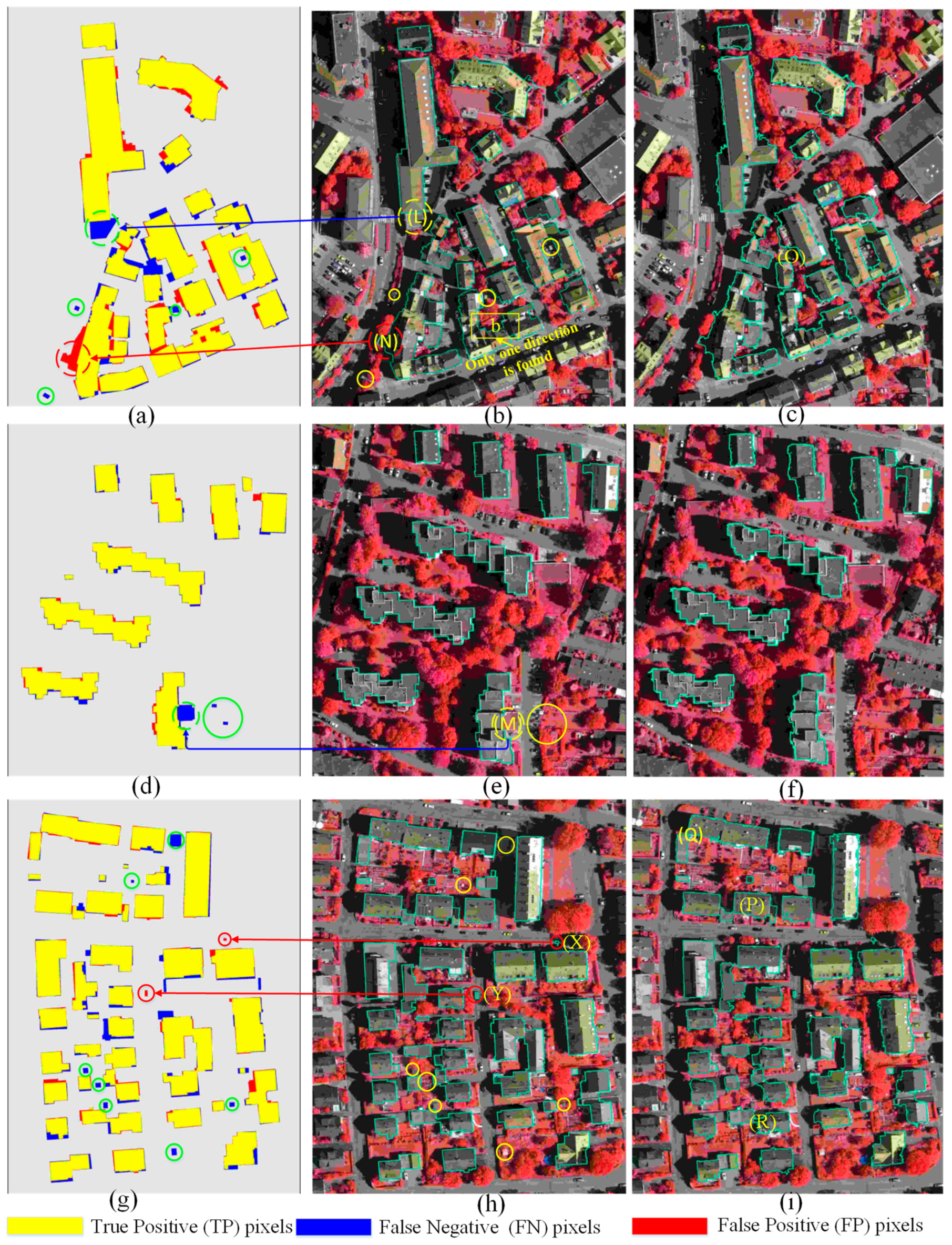
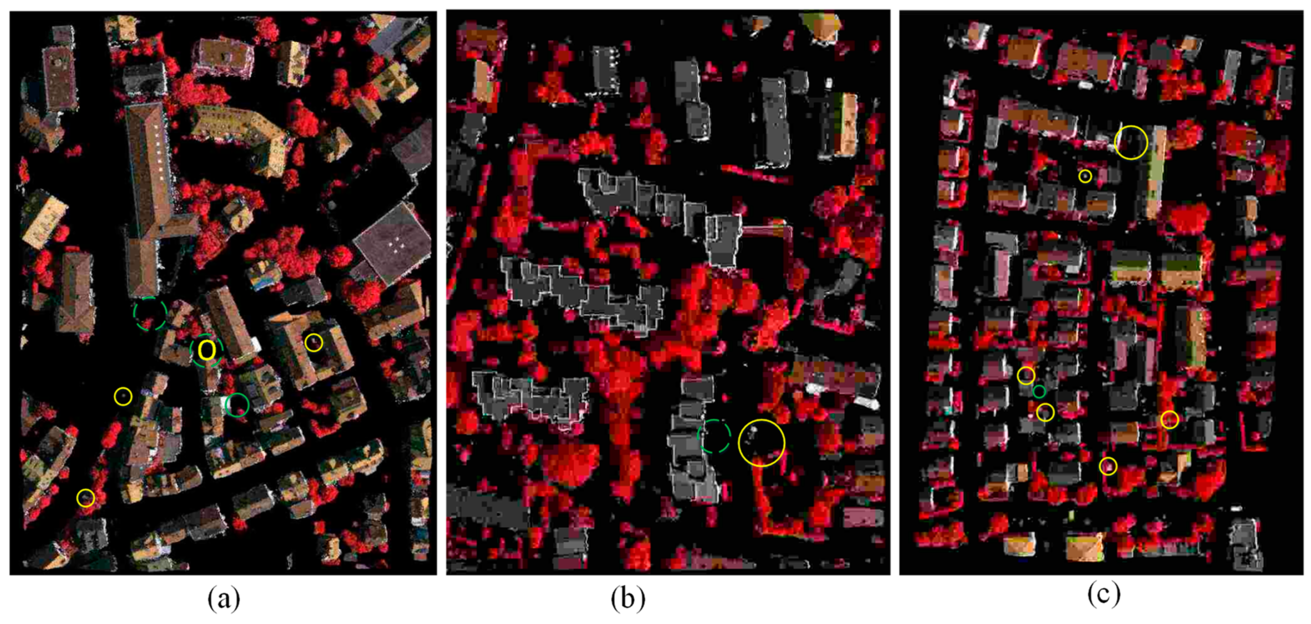
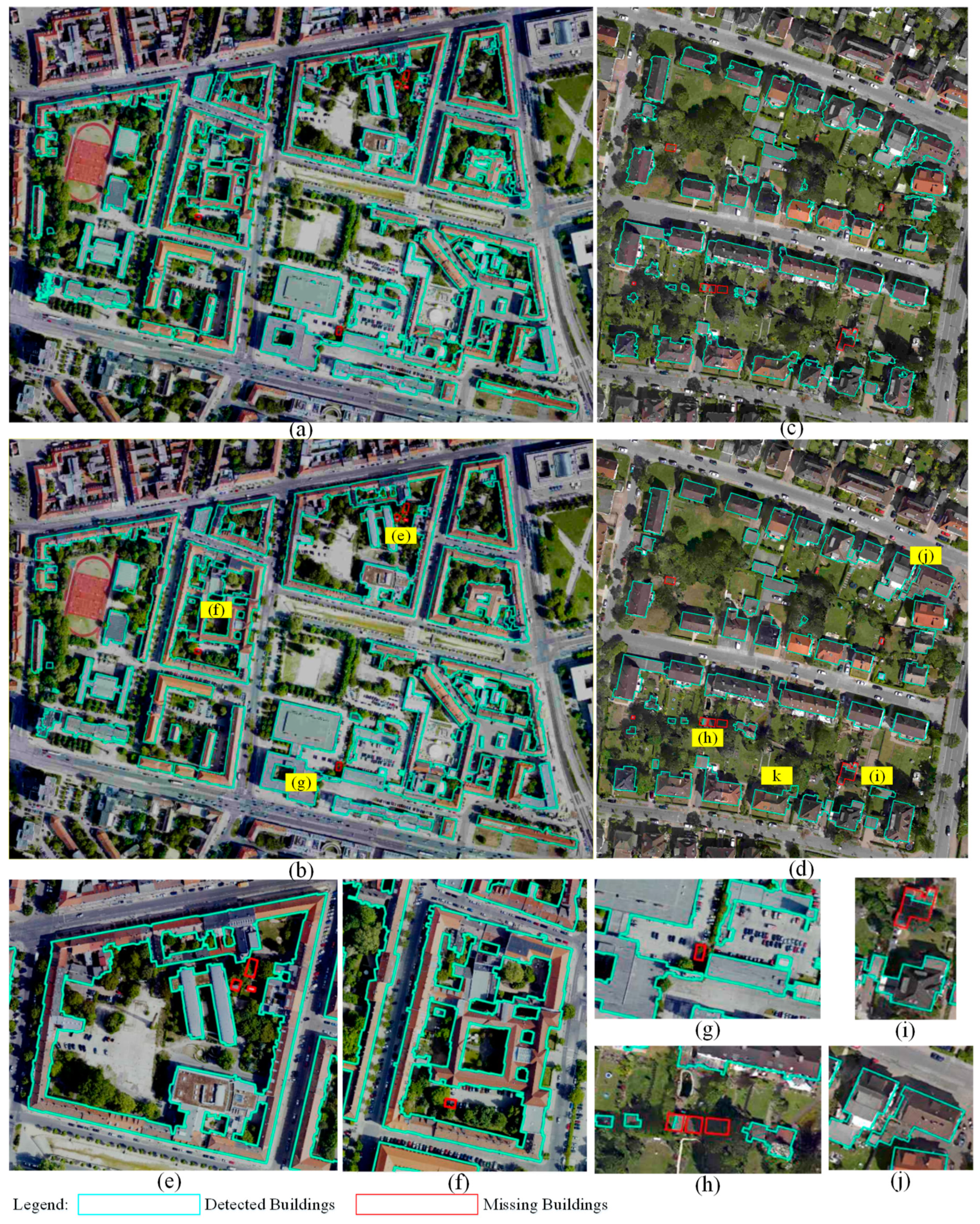
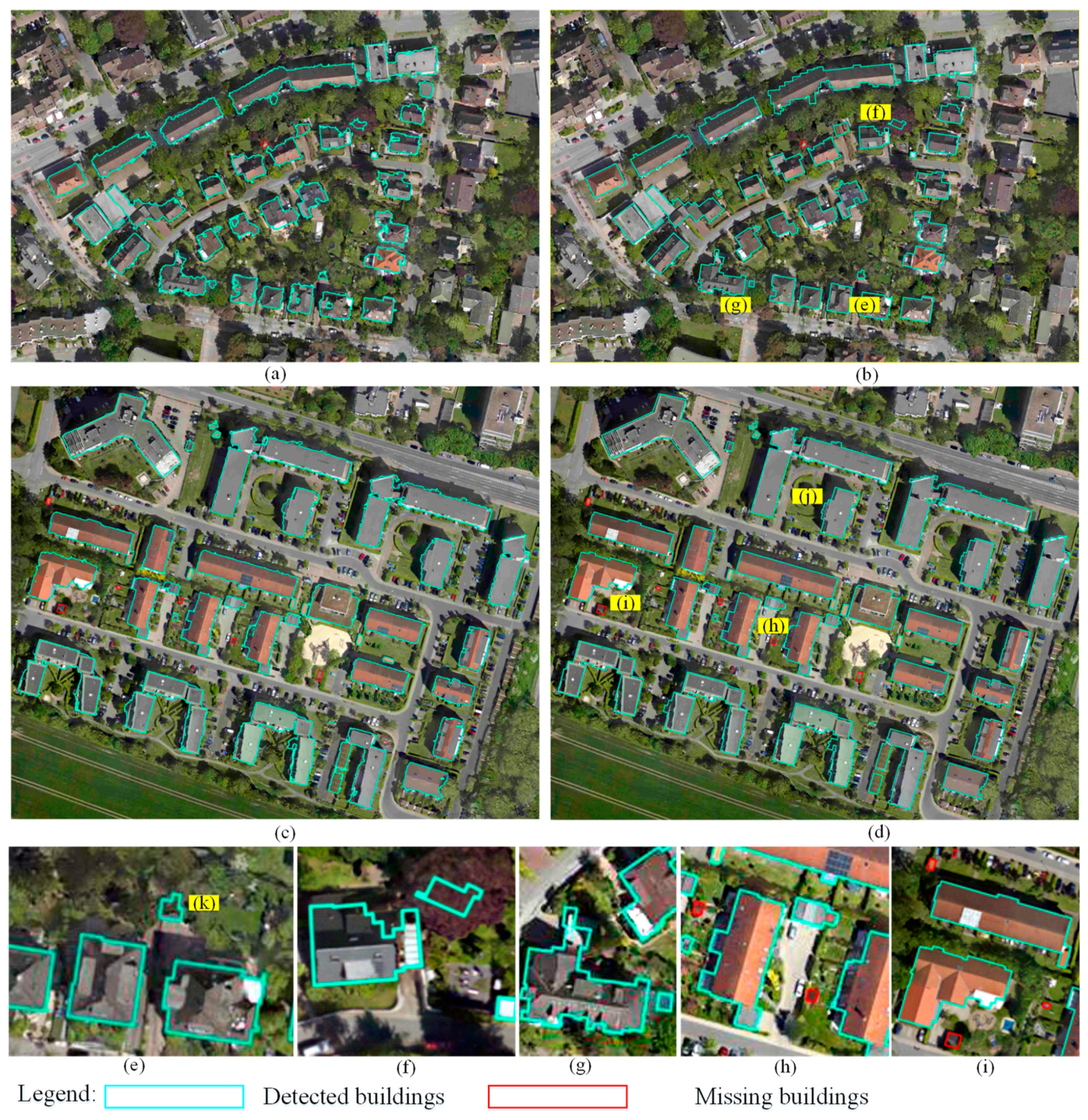
Table 1.
Symbol descriptions in the performance evaluation.
| Symbols | Description |
|---|---|
| m, m,50 | Completeness for all the buildings, over 50 2 and over 2.5 2 object-based detection |
| r, r,50 | Correctness for all the buildings, over 50 2 and over 2.5 2 object-based detection |
| l, l,50 | Quality for all the buildings, over 50 2 and over 2.5 2 object-based detection |
| mp, mp,50 | Completeness all the buildings, over 50 2 and over 2.5 2 pixel-based detection |
| rp, rp,50 | Correctness all the buildings, over 50 2 and over 2.5 2 pixel -based detection |
| lp | Quality of all building pixel-based detection |
| Planimetric accuracy in meters | |
| M detected buildings correspond to one building in the reference (over-segmented) | |
| A detected building corresponds to N buildings in the reference (under-segmented) | |
| Both over- and under-segmentation in the number of buildings |
Table 2.
Object-based building detection results on the VH dataset before and after the regularization stage.
Table 2.
Object-based building detection results on the VH dataset before and after the regularization stage.
| Method | Areas | m | r | m,50 | r,50 | l,50 | ||||
|---|---|---|---|---|---|---|---|---|---|---|
| Before regularization | VH 1 | 81.00 | 100.00 | 81.00 | 100.00 | 100.00 | 100.00 | 0 | 2 | 1 |
| VH 2 | 83.30 | 100.00 | 83.30 | 100.00 | 100.00 | 100.00 | 0 | 0 | 0 | |
| VH 3 | 87.20 | 95.23 | 81.60 | 100.00 | 100.00 | 100.00 | 0 | 2 | 0 | |
| Average | 83.83 | 98.41 | 81.97 | 100.00 | 100.00 | 100.00 | 0 | 1.33 | 0.33 | |
| After regularization | VH 1 | 81.00 | 100.00 | 81 | 100.00 | 100.00 | 100.00 | 0 | 2 | 1 |
| VH 2 | 83.30 | 100.00 | 83.3 | 100.00 | 100.00 | 100.00 | 0 | 0 | 0 | |
| VH 3 | 87.20 | 95.23 | 81.6 | 100.00 | 100.00 | 100.00 | 0 | 2 | 0 | |
| Average | 83.83 | 98.41 | 81.97 | 100.00 | 100.00 | 100.00 | 0 | 1.33 | 0.33 |
Table 3.
Pixel-based building detection results on the VH dataset before and after the regularization stage.
Table 3.
Pixel-based building detection results on the VH dataset before and after the regularization stage.
| Proposed Detection | Areas | mp | rp | lp | |
|---|---|---|---|---|---|
| Before regularization | VH 1 | 90.7 | 91.2 | 83.45 | 0.853 |
| VH 2 | 89.14 | 95.47 | 88.55 | 0.612 | |
| VH 3 | 90.42 | 95.22 | 86.5 | 0.727 | |
| Average | 90.09 | 93.96 | 86.17 | 0.731 | |
| After regularization | VH 1 | 90.38 | 92.29 | 84.04 | 0.844 |
| VH 2 | 92.37 | 96.75 | 89.59 | 0.591 | |
| VH 3 | 90.7 | 95.68 | 87.13 | 0.632 | |
| Average | 91.15 | 94.91 | 89.92 | 0.69 |
Table 4.
Object-based building detection results on the Potsdam and Lunen (LN) datasets before and after the regularization stage.
Table 4.
Object-based building detection results on the Potsdam and Lunen (LN) datasets before and after the regularization stage.
| Method | Areas | m | r | l | m,50 | r,50 | l,50 | |||
|---|---|---|---|---|---|---|---|---|---|---|
| Before regularization | Potsdam | 90.74 | 100 | 90.74 | 100 | 100 | 100 | 1 | 4 | 0 |
| 87.71 | 96.15 | 84.75 | 97.06 | 100 | 97.06 | 0 | 8 | 0 | ||
| 94.4 | 97.14 | 91.89 | 100 | 100 | 100 | 0 | 3 | 0 | ||
| 86.05 | 94.59 | 82.22 | 100 | 100 | 100 | 0 | 2 | 0 | ||
| Average | 89.73 | 96.97 | 87.4 | 99.27 | 100 | 99.27 | 0.25 | 4.25 | 0.25 | |
| After regularization | Potsdam | 90.74 | 100 | 90.74 | 100 | 100 | 100 | 1 | 3 | 0 |
| 87.71 | 96.15 | 84.75 | 97.06 | 100 | 97.06 | 0 | 8 | 0 | ||
| 94.4 | 97.14 | 91.89 | 100 | 100 | 100 | 0 | 2 | 1 | ||
| 86.05 | 94.59 | 82.22 | 100 | 100 | 100 | 0 | 2 | 0 | ||
| Average | 89.73 | 96.97 | 87.4 | 99.27 | 100 | 99.27 | 0.25 | 4.25 | 0.25 |
Table 5.
Pixel-based building detection results on the Potsdam and LN datasets before and after the regularization stage.
Table 5.
Pixel-based building detection results on the Potsdam and LN datasets before and after the regularization stage.
| Proposed Detection | Areas | mp | rp | lp | |
|---|---|---|---|---|---|
| Before regularization | Potsdam | 94.9 | 95.1 | 90.5 | 0.913 |
| 93.15 | 89.33 | 83.82 | 0.882 | ||
| 91.81 | 93.05 | 85.92 | 0.816 | ||
| 95.72 | 93.78 | 90 | 0.754 | ||
| Average | 93.9 | 92.82 | 87.56 | 0.841 | |
| After regularization | Potsdam | 94.61 | 95.7 | 90.76 | 0.843 |
| 93.32 | 90.02 | 84.56 | 0.813 | ||
| 92.3 | 94.12 | 87.27 | 0.742 | ||
| 96.4 | 93.69 | 90.52 | 0.715 | ||
| Average | 94.16 | 93.38 | 88.28 | 0.778 |
Table 6.
Six existing methods compared with our proposed technique.
| Benchmark Data Set | Methods | Data Type | Processing Strategy | Reference |
|---|---|---|---|---|
| VH | DLR | Image | supervised | [8] |
| RMA | Image | data-driven | [8] | |
| Hand | Image | Dempster-Shafer | [8] | |
| Fed_2 | LiDAR + image | data-driven | [39] | |
| ITCR | LiDAR + image | supervised | [17] | |
| MON4 | LiDAR + image | Data-driven | [28] |
Table 7.
Comparison of the results of different methods in Vaihingen.
| Area | Method | m | r | m,50 | r,50 | mp | rp | ||||
|---|---|---|---|---|---|---|---|---|---|---|---|
| VH1 | DLR | 83.8 | 96.9 | 100 | 100 | 91.9 | 95.4 | 0.9 | - | - | - |
| RMA | 83.8 | 96.9 | 100 | 100 | 91.6 | 92.4 | 1.0 | - | - | - | |
| Hand | 83.8 | 93.9 | 100 | 100 | 93.8 | 90.5 | 0.9 | - | - | - | |
| Fed_2 | 83.8 | 100 | 100 | 100 | 85.4 | 86.6 | 1.0 | 0 | 6 | 0 | |
| ITCR | 86.5 | 91.4 | 100 | 100 | 91.2 | 90.3 | 1.1 | - | - | - | |
| MON4 | 89.2 | 93.9 | 100 | 100 | 92.1 | 83.9 | 1.3 | - | - | - | |
| PM | 81 | 100 | 100 | 100 | 90.38 | 92.29 | 0.8 | 0 | 2 | 1 | |
| VH2 | DLR | 78.6 | 100 | 100 | 100 | 94.3 | 97 | 0.6 | - | - | - |
| RMA | 85.7 | 52.2 | 100 | 100 | 95.4 | 85.9 | 0.9 | - | - | - | |
| Hand | 78.6 | 78.6 | 100 | 100 | 95.1 | 89.8 | 0.8 | - | - | - | |
| Fed_2 | 85.7 | 100 | 100 | 100 | 88.8 | 84.5 | 0.9 | 0 | 2 | 0 | |
| ITCR | 78.6 | 42.3 | 100 | 100 | 94 | 89 | 0.8 | - | - | - | |
| MON4 | 85.7 | 91.7 | 100 | 100 | 97.2 | 83.5 | 1.1 | - | - | - | |
| PM | 83.8 | 100 | 100 | 100 | 92.37 | 96.75 | 0.6 | 0 | 0 | 0 | |
| VH3 | DLR | 78.6 | 100 | 100 | 100 | 93.7 | 95.5 | 0.7 | - | - | - |
| RMA | 78.6 | 93.9 | 100 | 100 | 91.3 | 92.4 | 0.8 | - | - | - | |
| Hand | 78.6 | 92.8 | 92.1 | 100 | 91.9 | 90.6 | 0.8 | - | - | - | |
| Fed_2 | 82.1 | 95.7 | 100 | 100 | 89.9 | 84.7 | 1.1. | 0 | 5 | 0 | |
| ITCR | 75 | 78.2 | 94.7 | 100 | 89.1 | 92.5 | 0.8 | - | - | - | |
| MON4 | 76.8 | 95.7 | 97.4 | 100 | 93.7 | 81.3 | 1.0 | - | - | - | |
| PM | 85.11 | 95.23 | 100 | 100 | 90.7 | 95.68 | 0.6 | 0 | 2 | 0 |
© 2018 by the authors. Licensee MDPI, Basel, Switzerland. This article is an open access article distributed under the terms and conditions of the Creative Commons Attribution (CC BY) license (http://creativecommons.org/licenses/by/4.0/).
Share and Cite
MDPI and ACS Style
Dong, Y.; Zhang, L.; Cui, X.; Ai, H.; Xu, B. Extraction of Buildings from Multiple-View Aerial Images Using a Feature-Level-Fusion Strategy. Remote Sens. 2018, 10, 1947. https://0-doi-org.brum.beds.ac.uk/10.3390/rs10121947
AMA Style
Dong Y, Zhang L, Cui X, Ai H, Xu B. Extraction of Buildings from Multiple-View Aerial Images Using a Feature-Level-Fusion Strategy. Remote Sensing. 2018; 10(12):1947. https://0-doi-org.brum.beds.ac.uk/10.3390/rs10121947
Chicago/Turabian StyleDong, Youqiang, Li Zhang, Ximin Cui, Haibin Ai, and Biao Xu. 2018. "Extraction of Buildings from Multiple-View Aerial Images Using a Feature-Level-Fusion Strategy" Remote Sensing 10, no. 12: 1947. https://0-doi-org.brum.beds.ac.uk/10.3390/rs10121947
Note that from the first issue of 2016, this journal uses article numbers instead of page numbers. See further details here.