Characterizing Variability of Solar Irradiance in San Antonio, Texas Using Satellite Observations of Cloudiness

Abstract

Since the main attenuation of solar irradiance reaching the earth’s surface is due to clouds, it has been hypothesized that global horizontal irradiance attenuation and its temporal variability at a given location could be characterized simply by cloud properties at that location. This hypothesis is tested using global horizontal irradiance measurements at two stations in San Antonio, Texas, and satellite estimates of cloud types and cloud layers from the Geostationary Operational Environmental Satellite (GOES) Surface and Insolation Product. A modified version of an existing solar attenuation variability index, albeit having a better physical foundation, is used. The analysis is conducted for different cloud conditions and solar elevations. It is found that under cloudy-sky conditions, there is less attenuation under water clouds than those under opaque ice clouds (optically thick ice clouds) and multilayered clouds. For cloud layers, less attenuation was found for the low/mid layers than for the high layer. Cloud enhancement occurs more frequently for water clouds and less frequently for mixed phase and cirrus clouds and it occurs with similar frequency at all three levels. The temporal variability of solar attenuation is found to decrease with an increasing temporal sampling interval and to be largest for water clouds and smallest for multilayered and partly cloudy conditions. This work presents a first step towards estimating solar energy potential in the San Antonio area indirectly using available estimates of cloudiness from GOES satellites.

1. Introduction

Radiation from the sun is the primary energy source for the Earth [1,2]. Accurate measurements of broadband shortwave irradiance are crucial for renewable energy resource assessments and climate change research [3]. There is also a growing demand for integrating solar energy into the electricity grid with accurate characterization of solar irradiance variability in order to provide a better quality of service. The temporal variability of solar radiation is largely due to rapid changes in atmosphere conditions, especially clouds, which create significant fluctuations in voltage [4,5,6,7,8,9]. The insolation, cloud amount, cloud type, cloud height, and surface properties determine whether clouds cause a radiative excess or deficit in a given region. Considering the importance of the stability of an energy distribution network and considering also that the reduction of solar radiation in the atmosphere due to clouds is typically larger (~30%) than that due to aerosols under clear sky (~10%) [10], it would be useful to understand how solar energy varies under different cloud conditions.

To quantify the effects of clouds on radiation at a specific location, a clear sky index (CSI) can be used [11,12,13]. The CSI is defined as the ratio of the actual ground irradiance to the irradiance under a cloud-free sky [14]. Thus, when calculating CSI, the selection of a good clear sky model is important. Reno et al. [15] presented an overview of clear sky models of global horizontal irradiance including very simple models that are solely dependent upon solar zenith angle and quite complex models that add dependencies on various atmospheric parameters. They found that the Ineichen model [16,17], which accounts for solar zenith angle, air pressure, temperature, relative humidity, aerosol content, Rayleigh and site elevation, compared well (error of ~5.0%) with the REST2 (Reference Evaluation of Solar Transmittance, 2-bands) model developed by Gueymard [18,19].

Cloud properties including cover, transmittance, moving velocity, type, and height, all influence solar irradiance and its variability on the ground [8,20,21,22,23,24]. Udelhofen and Cess [25] applied spectral analysis to cloud cover anomalies over the United States for the period 1900–1987 and found that the coherence between cloud cover and sun spots numbers (which is a proxy for solar variability) at a period of 11 years was significant (~0.7). Reno and Stein [23] hypothesized that the variability of cloud properties at a given location and time could be used to model the variability of ground solar irradiance at that location. Using global horizontal irradiance observations at two locations in Las Vegas, Nevada and cloud types from Geostationary Operation Environmental Satellites (GOES), they found that the temporal variability of ground irradiance is higher with water clouds and generally lower with opaque ice clouds. Nguyen et al. [26] validated the sky-imager-based global horizontal irradiance variability with ground observations using the temporal variability index introduced by Stein et al. [22] and found a high correlation (0.91).

Previously, we compared satellite-derived global solar irradiance from GOES with ground observations at two stations in San Antonio, Texas and found overall a good agreement on hourly and daily timescales [27]. The irradiance data from these two ground stations are used here to study the temporal variability of global horizontal irradiance on sub-hourly time scales. The specific objective of this study is to use the global horizontal irradiance measured at these two San Antonio sites and simultaneous GOES-derived cloud properties (i.e., cloud type and height) to test the hypothesis of Reno and Stein [23], namely that the global horizontal irradiance variability at these stations could be characterized by satellite-derived cloud properties at those locations. In addition, a modified version of the global horizontal irradiance variability index of Reno and Stein [23], but bearing a more physical foundation, is used here. In this paper, the datasets used are presented in Section 2, the analysis methods in Section 3, and the results in Section 4. The paper ends with a discussion in Section 5 and conclusions in Section 6.

2. Data

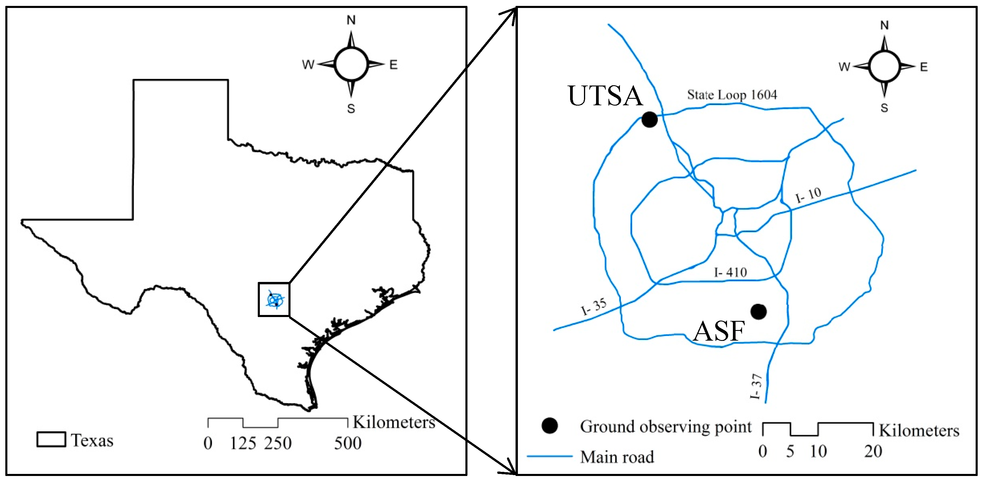
2.1. Ground Observations of Solar Irradiance

In situ measurements of global horizontal irradiance (G_h) come from the two ground stations shown in Figure 1, namely the main campus of the University of Texas at San Antonio (UTSA) and Alamo 1 Solar Farm (ASF). At the UTSA station (29.5833° N, 98.6199° W, 305 m elevation above sea level), instantaneous values of G_h were recorded every 5 min from 1 May to 25 October 2015 by a LI-200R pyranometer (0.4–1.1 µm). At the ASF site (29.7010° N, 98.4432° W, 164 m elevation above sea level), instantaneous values of G_h were recorded at irregular time intervals which is against best practices. The distribution of the sampling has a mean of 0.16 min and standard deviation of 0.23 min from July to September 2014 by a CMP11_L pyranometer (0.285–2.8 µm). A second ASF dataset based on temporal averages is used for the period September 2015–October 2016 in which the raw data was averaged every 15 min. The uncertainties of the instruments, LI-200R and CMP11_L, are respectively 3% and <2%, according to the manufacturer specifications. The bandwidth of the LI-200R pyranometer is much narrower than that of the CMP11_L pyranometer. Slight sensor differences in offset and/or gain and the pyranometer calibration at the UTSA station might have induced some errors, resulting in slightly smaller G_h than that recorded at the ASF station [27]. Since at large zenith angles the accuracies of radiative transfer models and pyranometers degrade rapidly [27], and slight changes in actual radiance can cause large changes in the clear sky index, observations with solar zenith angles >75° were, therefore, not included in this study.

2.2. Satellite Observations of Clouds

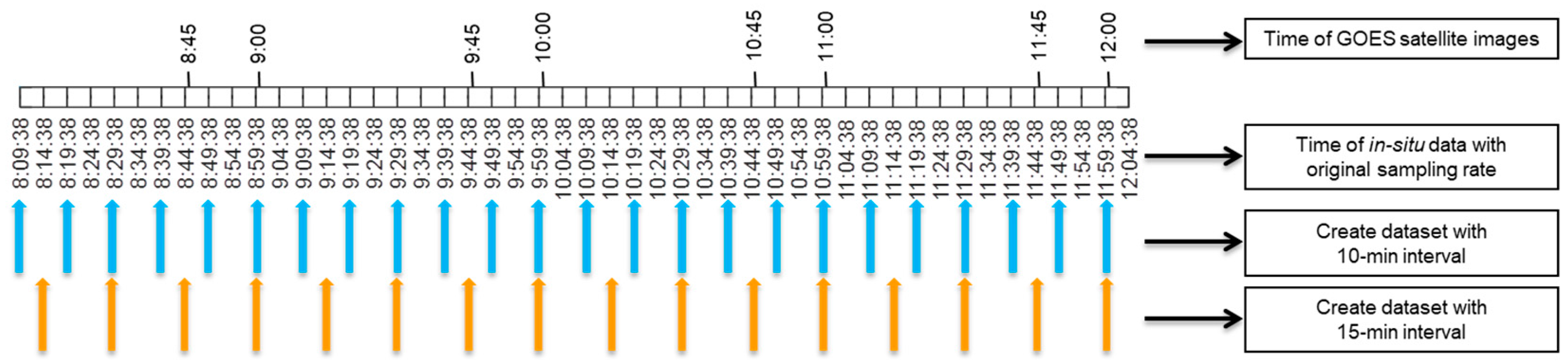
The satellite cloud data used in this paper comes from the GOES Surface and Insolation Products (GSIP) available from the National Oceanic Atmospheric Administration (NOAA). The GSIP dataset is based on remote sensing measurements obtained using the visible and infrared channels of the GOES satellites. Both GOES-East and GOES-West satellites are used, which respectively provide hourly instantaneous snapshots 45 min past the hour and on the hour since January 1996 [28]. The approach of GSIP for computing solar radiation is to first retrieve cloud properties and then use these properties as inputs to the Satellite Algorithm for Shortwave Radiation Budget (SASRAB) model [29]. The algorithm used to determine the dominant cloud types is the AVHRR Pathfinder Atmospheres-Extended (PATMOS-X) model [29,30,31]. In this study, hourly cloud property data (classified by cloud types and cloud layers, as defined in

Table 1. Cloud categories for National Oceanic Atmospheric Administration (NOAA) cloud-types (same categories used in Reference [23]) and cloud-layer classifications from Geostationary Operational Environmental Satellite (GOES) surface and insolation products.

Classification	Categories	Description
Cloud type	0	clear
	1	partly (partly cloudy/fog)
	2	water (water cloud)
	3	mixed (supercooled/mixed-phase cloud)
	4	opaque ice (optically thick ice cloud)
	5	cirrus (optically thin ice cloud)
	6	multilayered (cirrus over lower cloud)
Cloud layer	1	low (0–2 km)
	2	mid (2–7 km)
	3	high (5–13 km)

) with a resolution of 2.3 km (longitude) × 4.9 km (latitude) for San Antonio, Texas are obtained from GSIP.

3. Methods

Ground measurements of G_h with various sub-hourly temporal sampling intervals were used in this study. For UTSA, the sampling intervals considered were 5, 10, and 15 min and for ASF the sampling intervals were 1, 5, 10, and 15 min. For the UTSA data, the 10 and 15 min datasets (instantaneous data) were generated by decimating the original 5-min datasets so that the resulting grids match the times of the satellite imagery, as illustrated in Figure 2. For ASF, the 1, 5, and 10 min datasets were based on instantaneous data while the 15 min dataset was a combination of an instantaneous and a temporally averaged dataset. These four regularly gridded ASF datasets were generated in a similar way to the UTSA datasets by decimating the irregularly sampled high resolution (~0.16 min mean sampling rate) dataset using the nearest data to the desired regular grid which was chosen to match the times of the satellite imagery. When generating the 10-min gridded dataset one can choose to match the time of the satellite image 15 min before the hour or indistinctively the one on the hour, we chose the latter.

To quantify the impact of clouds on solar irradiance, a clear sky index (CSI) [11,14,32] was used as follows:

$$\mathrm{CSI}=\frac{{\mathrm{G}}_{\mathrm{h}}}{{\mathrm{G}}_{\mathrm{hc}}},$$

(1)

where G_hc is the global horizontal clear-sky irradiance. Thus, CSI should be approximately equal to 1 under clear-sky conditions and typically smaller than 1 when clouds are present. In this paper, G_hc was calculated from the following model based on Reference [15]:

$${\mathrm{G}}_{\mathrm{hc}}={\mathrm{a}}_1·{\mathrm{I}}_0·\sin \left(\mathrm{h}\right)·\exp \left(-{\mathrm{a}}_2·\mathrm{AM}·\left({\mathrm{f}}_{\mathrm{h}1}+{\mathrm{f}}_{\mathrm{h}2}·\left({\mathrm{T}}_{\mathrm{L}}-1\right)\right)\right)·\exp \left(0.01·{\mathrm{AM}}^{1.8}\right),$$

(2)

where ${\mathrm{I}}_0$ is the normal incidence extraterrestrial irradiance; h is the solar elevation angle, AM is the altitude corrected air mass [33], ${\mathrm{a}}_1$ = 5.09 × 10⁻⁵ × altitude + 0.868, ${\mathrm{a}}_2$ = 3.92 × 10⁻⁵ × altitude + 0.0387, ${\mathrm{f}}_{\mathrm{h}1}$ = exp(−altitude/8000), ${\mathrm{f}}_{\mathrm{h}2}$ = exp(−altitude/1250), and ${\mathrm{T}}_{\mathrm{L}}$ is Linke turbidity available from the Solar Radiation Data website (www.soda-pro.com). For every decimated G_h dataset (i.e., 1, 5, 10, or 15 min sampling rate), a corresponding G_hc dataset was generated by calculating G_hc only for those times when G_h was available. The CSI was then calculated from Equation (1) for all sampling rates and averaged over a 60-min period centered on the time of each satellite image.

A variation of the CSI, but for evaluating the impact of clouds on energy rather than irradiance and for comparisons using the satellite retrieved cloudiness, is introduced here. The new index is referred to as the clear-sky energy index (CEI) and is defined as the ratio of two integrals. The numerator is the integral over one hour centered around the time of each satellite image of an array of n global-horizontal radiant energy values observed at a temporal sampling interval $\Delta \mathrm{t}$ and the denominator is the same integral but computed using the calculated global-horizontal clear-sky irradiance from Equation (2), as follows:

$$\mathrm{CEI}=\frac{{{\displaystyle \sum }}_{\mathrm{k}=2}^{\mathrm{n}}(({\left({\mathrm{G}}_{\mathrm{h}}\right)}_{\mathrm{k}}+{\left({\mathrm{G}}_{\mathrm{h}}\right)}_{\mathrm{k}-1})\ast \Delta \mathrm{t}/2)}{{{\displaystyle \sum }}_{\mathrm{k}=2}^{\mathrm{n}}(({\left({\mathrm{G}}_{\mathrm{hc}}\right)}_{\mathrm{k}}+{\left({\mathrm{G}}_{\mathrm{hc}}\right)}_{\mathrm{k}-1})\ast \Delta \mathrm{t}/2)}.$$

(3)

To evaluate the impact of clouds on the temporal variability of solar irradiance, the following variability index (VI) was used [22,23] which was calculated from an equation similar to Equation (3), as follows:

$$\mathrm{VI}=\frac{{{\displaystyle \sum }}_{\mathrm{k}=2}^{\mathrm{n}}\sqrt{{({\left({\mathrm{G}}_{\mathrm{h}}\right)}_{\mathrm{k}}-{\left({\mathrm{G}}_{\mathrm{h}}\right)}_{\mathrm{k}-1})}^2+\Delta {\mathrm{t}}^2}}{{{\displaystyle \sum }}_{\mathrm{k}=2}^{\mathrm{n}}\sqrt{{({\left({\mathrm{G}}_{\mathrm{hc}}\right)}_{\mathrm{k}}-{\left({\mathrm{G}}_{\mathrm{hc}}\right)}_{\mathrm{k}-1})}^2+\Delta {\mathrm{t}}^2}}.$$

(4)

As seen in Equation (4), the definition of VI involves adding variables with different units (i.e., energy flux for irradiance and time for the temporal sampling interval) which does not have any physical basis. To avoid this inconsistency, we proposed a modified version of the variability index (VI_new) defined as follows:

$${\mathrm{VI}}_{\mathrm{new}}=\frac{{{\displaystyle \sum }}_{\mathrm{k}=2}^{\mathrm{n}}|{\left({\mathrm{G}}_{\mathrm{h}}\right)}_{\mathrm{k}}-{\left({\mathrm{G}}_{\mathrm{h}}\right)}_{\mathrm{k}-1}|/\Delta \mathrm{t}}{{{\displaystyle \sum }}_{\mathrm{k}=2}^{\mathrm{n}}|{\left({\mathrm{G}}_{\mathrm{hc}}\right)}_{\mathrm{k}}-{\left({\mathrm{G}}_{\mathrm{hc}}\right)}_{\mathrm{k}-1}|/\Delta \mathrm{t}}.$$

(5)

This variability index was thus based on the ratio of the sum of the changes of global horizontal irradiance (in absolute value) over each time $\Delta \mathrm{t}$ taken over one hour centered on the time of each satellite image to the same sum quantity except computed for clear sky. The numerator one of the absolute value of the changes of observed ground global horizontal irradiance over each Δt and the other integral same quantity but based on the global horizontal irradiance under clear sky. The VI_new in Equation (5) is thus a modified version of the VI proposed by Reno and Stein [23]. This definition is very similar to the previous one given in Equation (4) but avoids the inconsistency of adding values with different units.

All solar radiation indices (CSI, CEI, VI, and VI_new) were then paired with simultaneous satellite estimates of clouds for further analysis [23].

4. Results

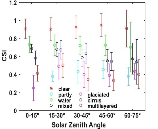
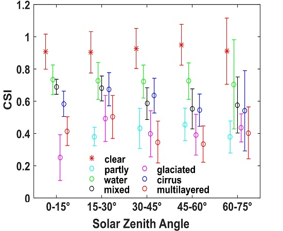
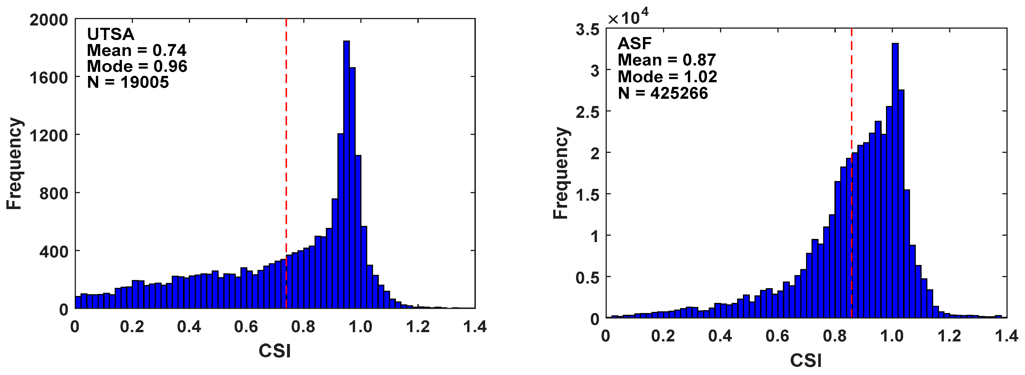
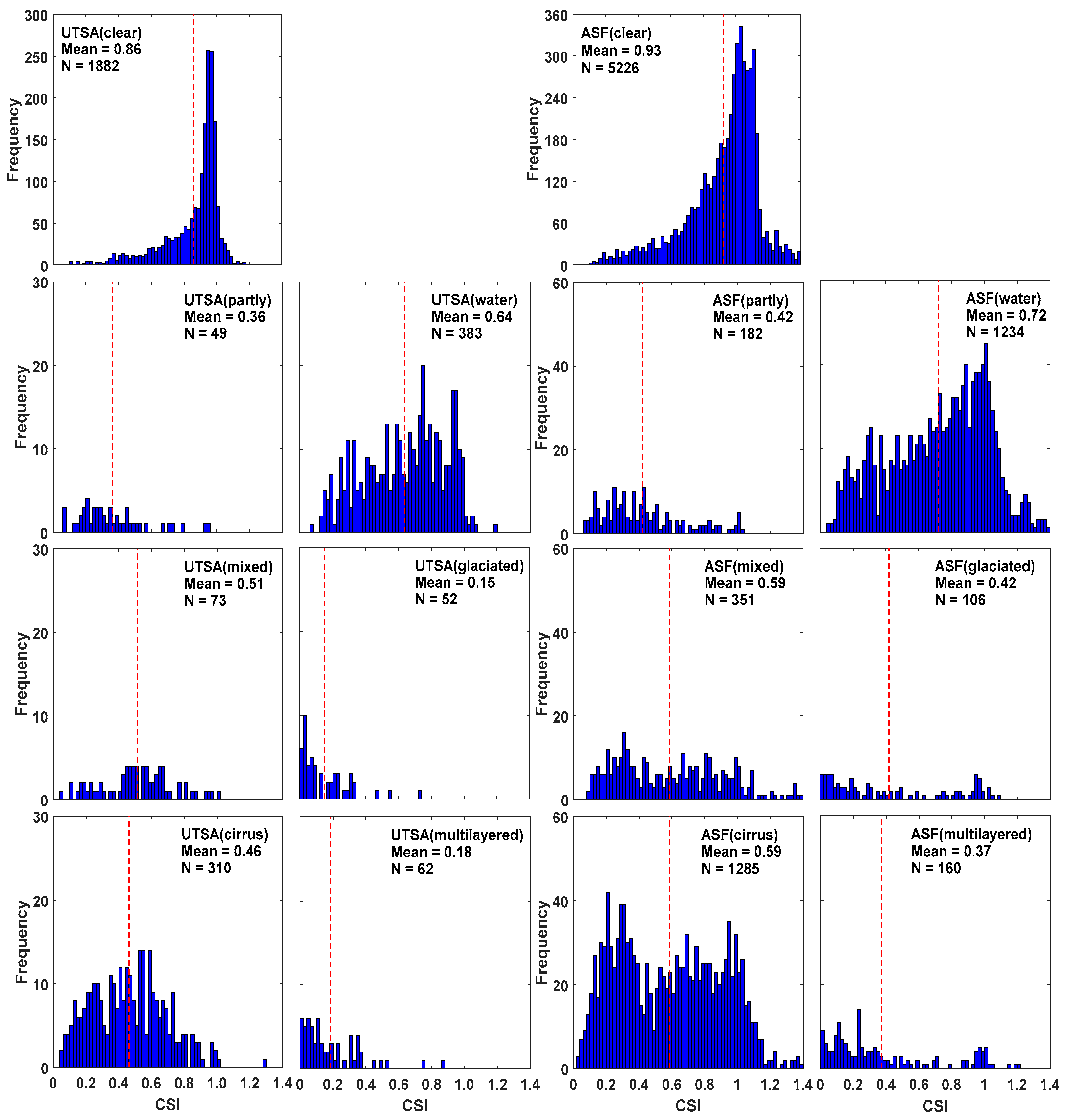
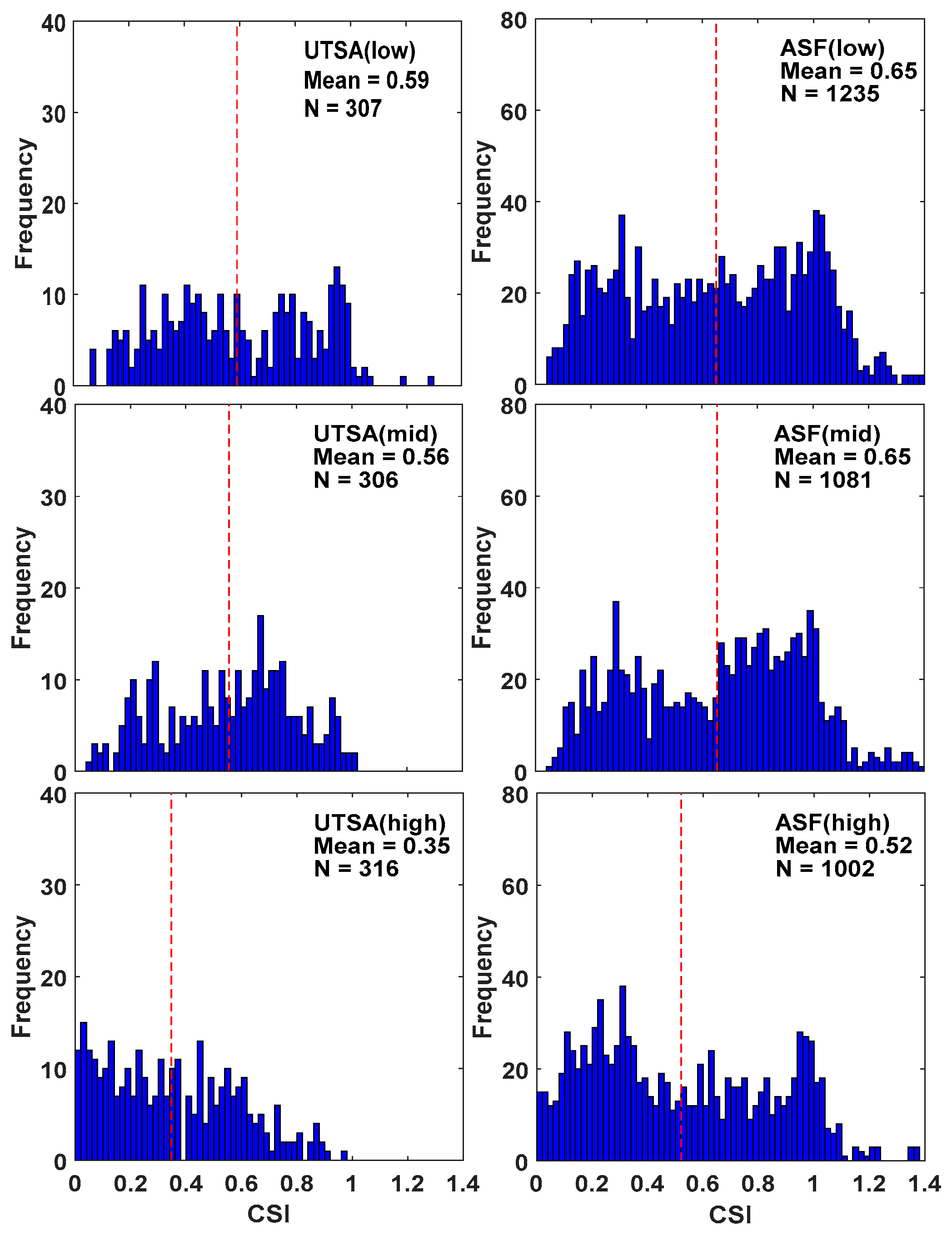
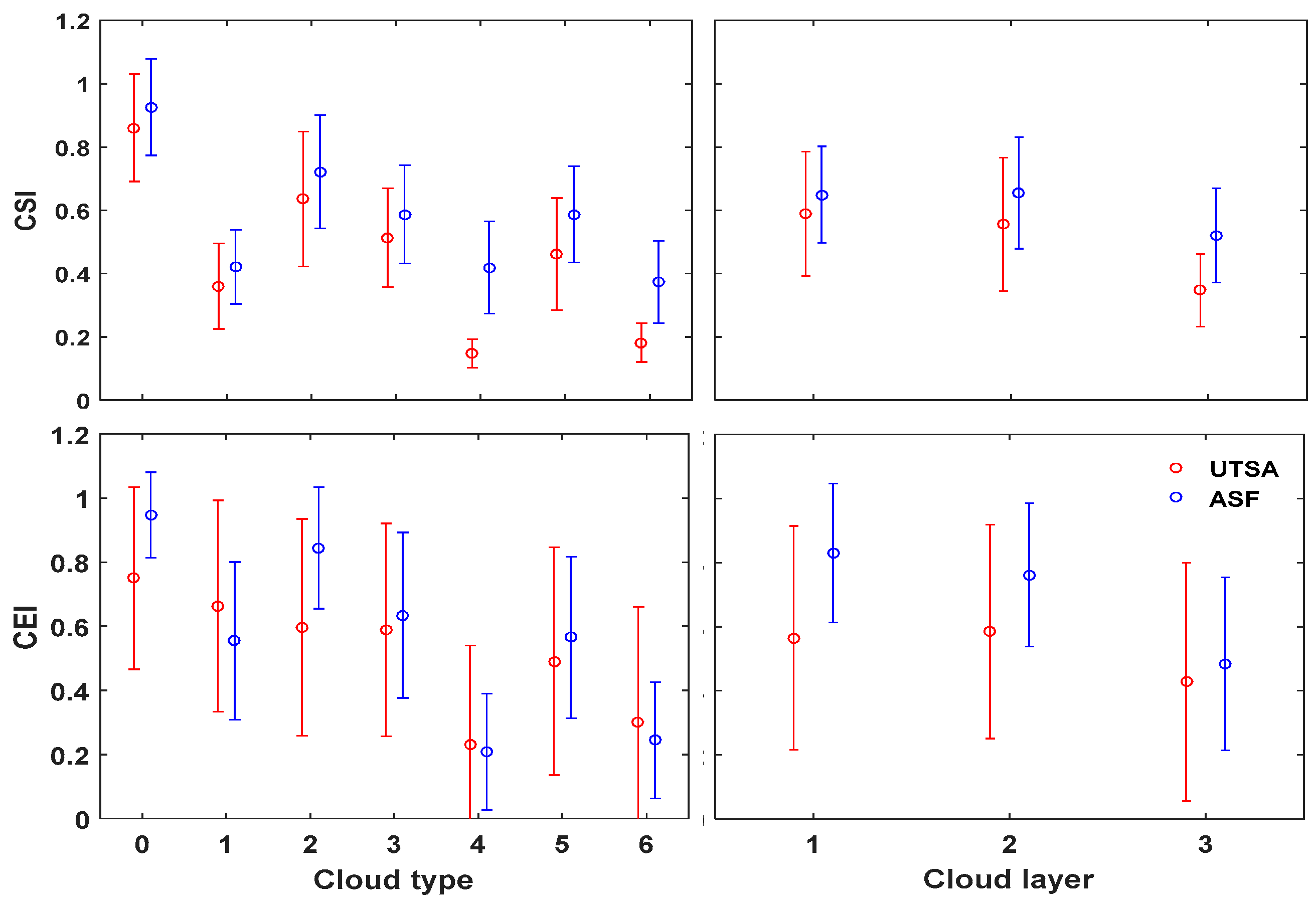
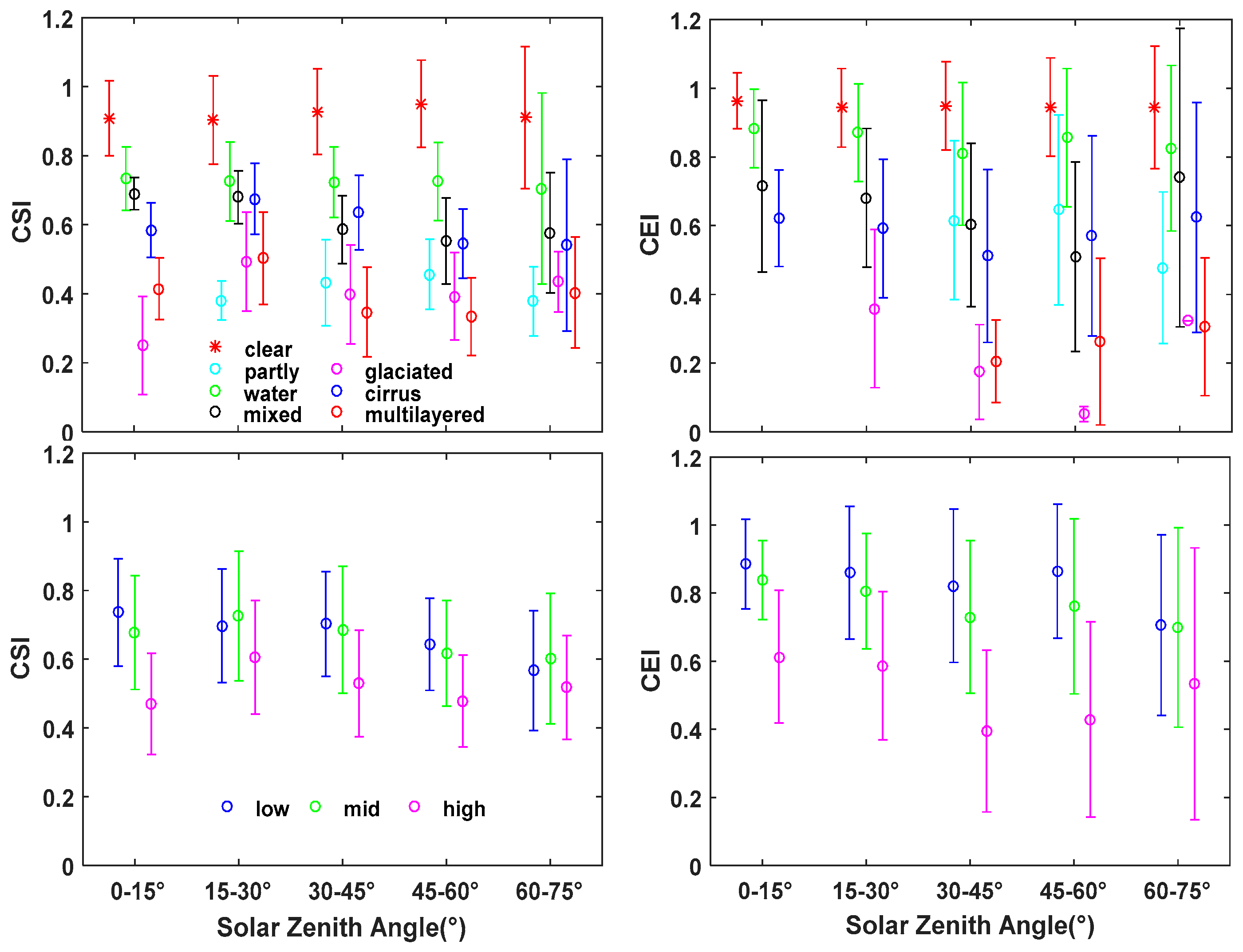
4.1. Solar Attenuation under Different Cloud Conditions

Figure 3 presents the histograms of CSI at the UTSA (left panel) and ASF (right panel) study sites using all available ground data and their original sampling rates. The means of these CSI distributions are 0.74 and 0.87 for UTSA and ASF, respectively, and are indicated with red vertical dashed lines in Figure 3. The modes of CSI are, respectively, 0.96 and 1.02 for UTSA and ASF. In principle, the maximum value of CSI would be equal to 1 which represents clear-sky conditions, i.e., solar irradiance should not be attenuated when passing through a clear atmosphere. The fact that some CSI values in Figure 3 are greater than 1 may be associated with (1) a possible underestimation of the clear sky global radiation (G_hc) from Equation (2) and/or (2) a possible overestimation of the ground measurements (G_h) at both stations due to cloud enhancement [34,35]. Both CSI distributions peak at 1 and are left-skewed indicating that there were more clear-sky than cloudy conditions at both locations.

The histograms of the averaged CSI values calculated using all available ground station data and the original sampling rates at the two study locations and for each cloud type are shown in Figure 4. Similar histograms, but for each cloud layer, are shown in Figure 5. Overall, two main conclusions can be drawn from these figures: (1) the distributions of CSI under clear-sky conditions in the upper panels of Figure 4 (>61% of all cases in both UTSA and ASF) peak at 1 and their average is greater than that for any cloud type or layer and (2) the mean of CSI is higher at ASF than at UTSA for all corresponding cloud types and layers. Among the various cloud types, water clouds have the larger CSI values, as shown in Figure 4. Values of CSI greater than 1 for clear-sky conditions reflect uncertainties in the CSI estimates since aerosols cannot enhance solar radiation. For cloudy conditions, CSI values greater than 1 are found more frequently for water clouds and less frequently for mixed and cirrus clouds suggesting that these cloud types are the most effective at producing cloud enhancement.

Among the three different cloud layers, CSI values are larger for low- and mid-level clouds than for high-level clouds, as shown in Figure 5. The water clouds are composed of liquid water droplets and the mixed clouds composed of supercooled water droplets or both ice and supercooled water. The water clouds absorb more visible and near-infrared radiation, resulting in lower CSI as compared to the clear-sky conditions [36,37,38]. Compared to water clouds, mixed clouds consist of water vapor, liquid droplets, and ice particles, and thus reflect more solar radiation and result in lower CSI. Cirrus clouds are higher-altitude, thinner clouds which are highly transparent to shortwave radiation. Partly cloudy conditions, in contrast, occur at the lower layer and are much thicker than cirrus clouds. The mean CSI, therefore, is higher under cirrus clouds than under partly cloudy conditions. The opaque ice clouds are composed of ice crystals or opaque clouds which are non-transmissive. The multilayer clouds consist of clouds from different layers. Both opaque ice and multilayer clouds reflect or absorb most of the solar energy, resulting in lower CSI than any other cloud type. It was also found that the distributions of CSI under clear and water cloud conditions are left skewed, while under cirrus clouds the distribution appears to be bimodal. Regarding cloud enhancement, the ASF data indicates that cloud enhancement occurs with similar frequency at all three levels.

Figure 6 shows the mean CSI and CEI with their standard deviation error bars under each cloud type and cloud layer for both stations. Similar to Figure 4 and Figure 5, CSI averages vary more as a function of cloud types than cloud layers and are higher at ASF than at UTSA. CSI is larger under clear-sky conditions (type 0) followed by water clouds (type 2) and lower under opaque ice (type 4) and multilayered (type 6) clouds. For cloud layers, CSI is larger for low and mid clouds (layers 1 and 2) and smaller for high clouds (layer 3). As expected, the pattern of CEI is similar to that of CSI. One difference, however, is that CEI is not always larger at ASF.

Figure 7 shows the mean CSI and CEI with their ± 1 standard deviation error bars for various sky conditions as a function of solar zenith angles at the ASF station. The distributions of CSI and CEI means and standard deviations in Figure 7 show both similarities and differences. Both CSI and CEI means are larger for clear than for cloudy conditions and they do not vary much with solar zenith angles. For cloudy conditions, the larger values of CSI and CEI means are for water clouds and the lower values for opaque ice and multilayered clouds. For CSI under partly, water, mixed, and cirrus type clouds, the means are generally lower at high solar zenith angles except for opaque ice clouds which have the lowest value of CSI at the lowest solar zenith angle (0–15°). For CEI under water, mixed, opaque ice, and cirrus, the means show smaller values for intermediate solar zenith angles. For cloud layers, as shown in the lower panel of Figure 7, the mean CSI decreases with increasing solar zenith angle for zenith angles greater than 0–15°. This pattern is similar for CEI which is overall higher at low, compared to high, solar zenith angles.

With respect to CSI and CEI under clear-sky conditions, their values are nearly 1 and do not change much with zenith angle. For cloud types and layers, CSI may increase (e.g., opaque ice) or decrease (e.g., mixed) with increasing solar zenith angle. For CEI under cloudy conditions (both for cloud types and layers), the attenuation is generally higher at higher solar zenith angles (>45°).

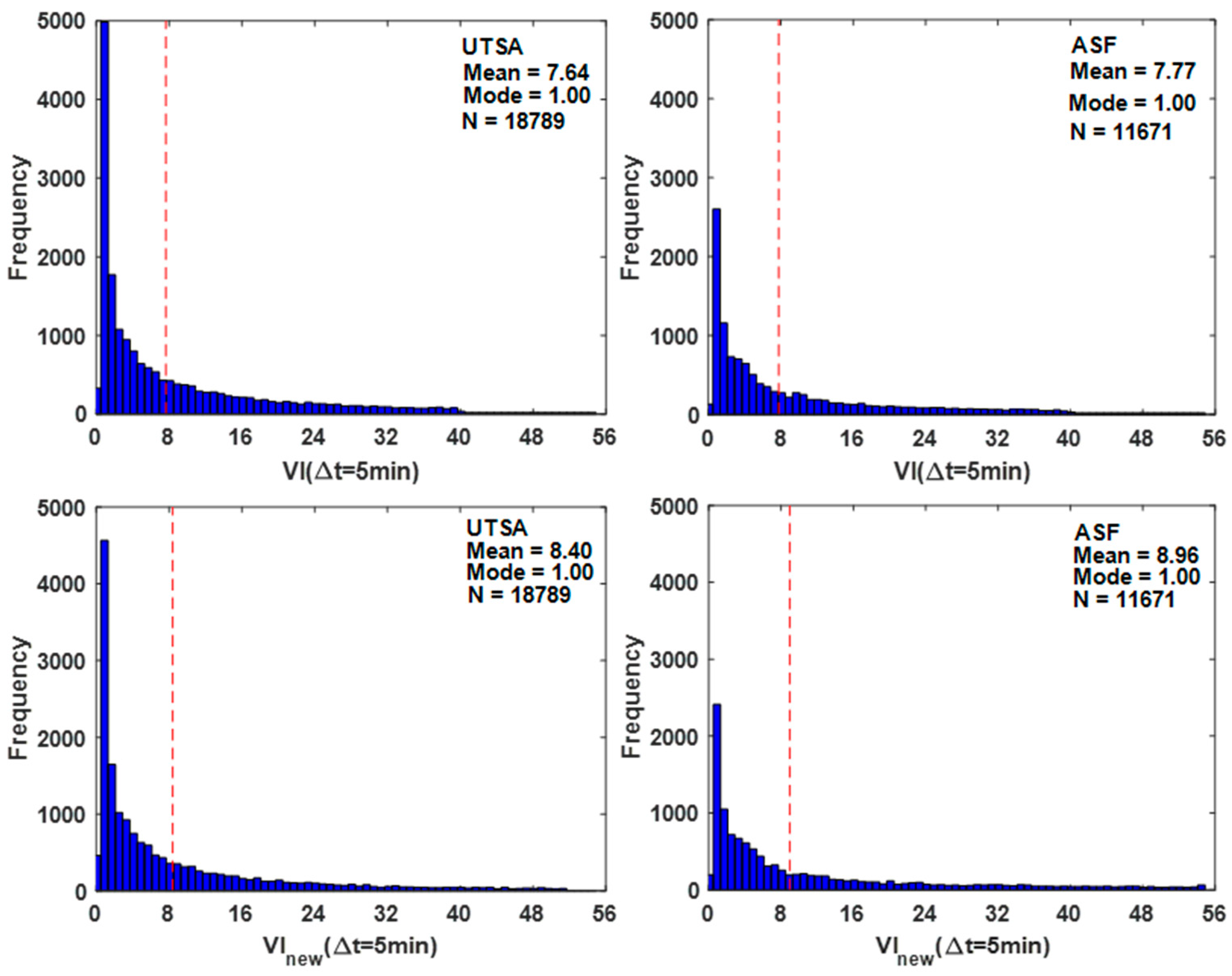
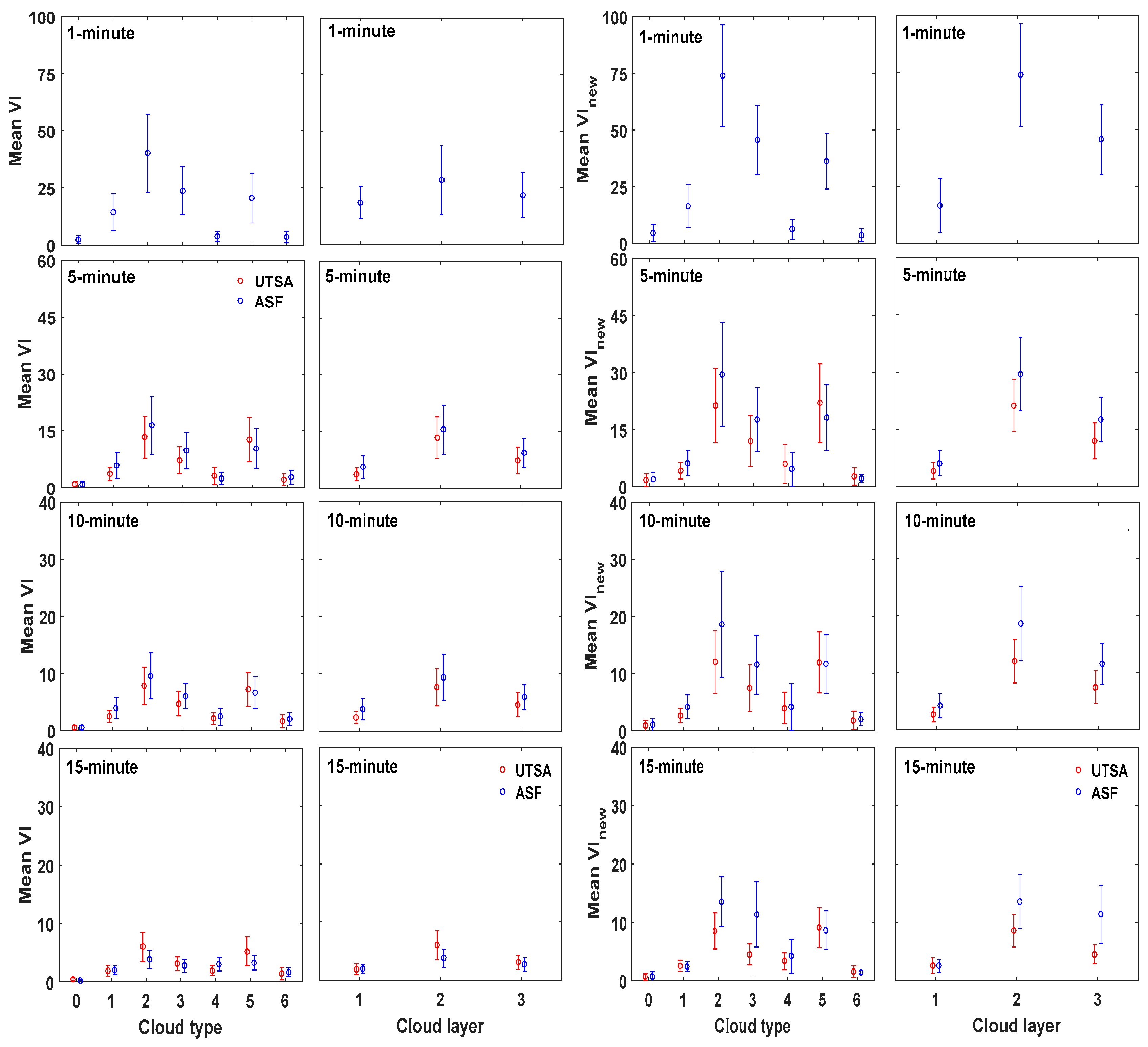
4.2. Temporal Variability of Solar Attenuation under Different Cloud Conditions

Figure 8 shows the histograms of the temporal variability indices VI and VI_new calculated using all data available at the two stations with the 5-min sampling interval, indicating that these distributions are quite similar to each other. The means of VI are, respectively, 7.64 and 7.77 for UTSA and ASF stations, while the means of VI_new are, respectively, 8.40 and 8.96 for UTSA and ASF. The modes of VI and VI_new for the two stations are all equal to 1. Both means of VI and VI_new are somewhat higher at the ASF station compared to the UTSA station. This is consistent with the results of Xia et al. [27] which found that the measured G_h values at the UTSA station were overall biased low, due in part to improper calibration of the pyranometer at that site. The right-skewed distribution of the variability indices peaking close to 1 indicates that there were more cases with low temporal variability than those with high temporal variability in the study sites.

Figure 9 shows the means ±1 standard deviation error bars of the temporal variability indices (VI and VI_new) in terms of cloud types and layers under different time intervals (1-min, 5-min, 10-min, and 15-min). Clearly, the temporal variability as represented by both indices decreases with the increase of time interval. In addition, VI shows smaller values than VI_new under different cloud types and layers, especially at the 10-min and 15-min time intervals. It appears that the physically based VI_new is more sensitive to cloud type changes than VI for the four time intervals in this study and is thus recommended for future use. For cloud types, VI_new shows high temporal variability under water clouds (type 2) and low solar variability under clear sky (type 0), opaque ice (type 4), and multilayered clouds (type 6). For cloud layers, VI_new shows high solar variability under mid clouds and low solar variability under low clouds, which are reasonable results.

5. Discussion

Different approaches have been used in the literature to study solar variability and its impact on the electricity grid [22,23,26,39,40,41]. For a review that includes various definitions of solar variability indices, the reader is referred to Reference [24]. In this study, we followed an approach similar to Reno and Stein [23] who used global horizontal irradiance at two ground stations in Las Vegas, Nevada and cloud types from GOES satellites. Here, the relationship between ground observations of global horizontal irradiance at two stations in San Antonio, Texas and satellite-derived cloud types and cloud layers from GOES satellites was investigated using both the same and modified attenuation and attenuation variability indices used in Reference [23].

This study found similar distributions of CSI at the two ground stations, namely ASF and UTSA, but the mean of these distributions differed slightly in magnitude with the ASF means being somewhat larger than those at UTSA, as shown in Figure 3, Figure 4 and Figure 5. These differences were attributed by Xia et al. [27] to the larger spectral band of the ASF pyranometer compared to the one at UTSA and to potential improper calibration of the pyranometer at the UTSA site. It is worth noticing that the CSI distributions in Figure 3, Figure 4 and Figure 5 show some values that are greater than 1, which may be attributed to possible underestimation of G_hc and/or overestimation of G_h due cloud enhancement [34,42,43]. Assuming that the CSI values greater than 1 for cloudy conditions in the ASF data represent cloud enhancement, more cloud enhancement is produced by water clouds and in lesser degree by mixed phase and cirrus clouds. In addition, cloud enhancement occurs at all three levels.

In Figure 3, Figure 4 and Figure 5, opaque ice and multilayered clouds have smaller CSI means because they contained ice crystals and opaque clouds resulting in high attenuation of solar radiation. The thin characteristics of cirrus clouds resulted in a lower ability to attenuate solar radiation as compared to opaque ice and multilayered clouds. Since there are more water clouds occurring at the lower layer and more opaque ice clouds at the high layer, the mean CSI is higher at the lower layer than at the higher layer.

Reno and Stein [23] found that at two locations in Las Vegas, Nevada the attenuation of solar radiation when arranged by cloud types according to CSI values from highest to lowest was clear, partly, water, cirrus, mixed, opaque ice, and multilayered. This organization is overall similar to the results of this study, except for partly-cloudy conditions. This study shows that the mean CSI for partly cloudy conditions is intermediate between mixed and opaque ice clouds, while for Reno and Stein [23] it is between clear sky and water clouds. These differences could be in part because their analysis was based on a coarser window of four by four GOES pixels, which could mix cloud types.

As expected, the attenuation indices CSI and CEI for clear-sky conditions, as shown in Figure 7, had larger values than for cloudy conditions and were nearly constant at all solar zenith angles due to the smaller attenuation of solar radiation in a cloud-free atmosphere compared to a cloudy atmosphere. Under cloudy-sky conditions, there was generally a decrease in CSI and CEI with increasing solar zenith angles. This effect was also expected since the longer the path that solar radiation travels through the cloudy atmosphere, the more the attenuation that would result.

The temporal variability of solar attenuation, as shown in Figure 9, is found to be dependent upon the temporal sampling interval with the mean variability indices (VI and VI_new) decreasing with the increase of the temporal sampling interval, consistent with Stein et al. [22]. The sampled ASF dataset at 15-min time interval could introduce errors due to the irregular temporal resolution. The variability indices of solar attenuation were lower under clear, partly, opaque ice, and multilayered clouds compared to those under water, mixed, and cirrus clouds. Of these last three, solar attenuation variability indices were higher for water clouds followed by mixed and cirrus clouds. All in all, these effects of clouds on attenuation variability are consistent with Reference [23].

6. Conclusions

Solar variability is considered a growing concern when it comes to the integration of the power from solar panel systems into the electric grid. Variation of solar irradiance at ground level results in variations of the harnessed solar power. The characterization of solar variability is thus very important for grid-connected solar photovoltaics and its impact on the power grid. A good understanding of short-term and long-term solar variability could contribute to grid reliability, power output forecast, and cost reduction.

In this paper, ground-based G_h observations and satellite-derived cloud properties were combined using attenuation (CSI, CEI) and attenuation variability (VI, VI_new) indices with the purpose of determining how solar radiation variability relates to cloud types and layers in San Antonio, Texas. As expected, it was found that on average solar radiation is attenuated the least under clear-sky conditions, followed by water clouds and cirrus clouds, and it is attenuated the most under opaque ice and multilayered clouds. Regarding cloud enhancement, the results suggest that it occurs more frequently under water clouds and less frequently for mixed phase and cirrus clouds. Cloud enhancement also appears to occur at all levels in the atmosphere. A new method was proposed for calculating the attenuation variability index (VI_new), which could be interpreted as the ratio of the rate of change of the observed global horizontal irradiance at some temporal sampling interval to the same quantity but computed from the global horizontal irradiance under clear sky. This definition makes more physical sense than the “length” approach posed by Reno and Stein [23], although gives similar results. The variability indices were found to decrease with increasing temporal sampling interval and were higher under water and mixed clouds and lower under opaque ice and multilayered clouds.

The results from this analysis illustrate how cloud classification from GOES satellites relates to solar attenuation and its temporal variability in San Antonio, Texas. It remains to be determined if these results could be extended to other regions. It remains also to be seen if similar results could be obtained using cloud products from other geostationary satellites like Meteosat or Himawari. The results of this study are overall consistent with the study of Reno and Stein [23] for Las Vegas, Nevada, but there are some differences. These differences, however, may be due to the different spatial resolution of the cloud datasets in the two studies rather than differences in optical properties of the clouds at the two sites.

The attenuation of solar radiation due to clouds has many uncertainties. This study, therefore, makes assumptions that are not able to be quantified, like cloud enhancement. An alternative way of studying the impact of clouds on solar irradiance would be using the optical properties of clouds in terms of optical thickness. The GOES dataset used here, if fact, uses the cloud optical thickness to parameterize the clouds. Some examples of studying the impact of clouds on solar irradiance using optical thickness include References [44,45,46].

References

1. Atri, D.; Melott, A.L. Cosmic rays and terrestrial life: A brief review. Astropart. Phys. 2014, 53, 186–190. [Google Scholar] [CrossRef] [Green Version]
2. Hosenuzzaman, M.; Rahim, N.A.; Selvaraj, J.; Hasanuzzaman, M.; Malek, A.B.M.A.; Nahar, A. Global prospects, progress, policies, and environmental impact of solar photovoltaic power generation. Renew. Sust. Energy Rev. 2015, 41, 284–297. [Google Scholar] [CrossRef]
3. Reda, I.; Stoffel, T.; Myers, D. A method to calibrate a solar pyranometer for measuring reference diffuse irradiance. Sol. Energy 2003, 74, 103–112. [Google Scholar] [CrossRef]
4. Hodge, B.-M.; Milligan, M. Wind power forecasting error distributions over multiple timescales. In Proceedings of the 2011 IEEE Power and Energy Society General Meeting, Detroit, MI, USA, 24–29 July 2011; pp. 1–8. [Google Scholar]
5. Lappalainen, K.; Valkealahti, S. Output power variation of different PV array configurations during irradiance transitions caused by moving clouds. Appl. Energy 2017, 190, 902–910. [Google Scholar] [CrossRef]
6. Lave, M.; Kleissl, J. Solar variability of four sites across the state of Colorado. Renew. Energy 2010, 35, 2867–2873. [Google Scholar] [CrossRef]
7. Lave, M.; Kleissl, J.; Arias-Castro, E. High-frequency irradiance fluctuations and geographic smoothing. Sol. Energy 2012, 86, 2190–2199. [Google Scholar] [CrossRef]
8. Lave, M.; Kleissl, J.; Stein, J.S. A wavelet-based variability model (WVM) for solar PV power plants. IEEE Trans. Sustain. Energy 2013, 4, 501–509. [Google Scholar] [CrossRef]
9. Moumouni, Y.; Baghzouz, Y.; Boehm, R.F. Power “smoothing” of a commercial-size photovoltaic system by an energy storage system. In Proceedings of the 16th International Conference on Harmonics and Quality of Power (ICHQP), Bucharest, Romania, 25–28 May 2014; pp. 640–644. [Google Scholar]
10. Valero, F.P.J.; Minnis, P.; Pope, S.K.; Bucholtz, A.; Bush, B.C.; Doelling, D.R.; Smith, W.L.; Dong, X. Absorption of solar radiation by the atmosphere as determined using satellite, aircraft, and surface data during the Atmospheric Radiation Measurement Enhanced Shortwave Experiment (ARESE). J. Geophys. Res. Atmos. 2000, 105, 4743–4758. [Google Scholar] [CrossRef] [Green Version]
11. Beyer, H.G.; Costanzo, C.; Heinemann, D. Modifications of the Heliosat procedure for irradiance estimates from satellite images. Sol. Energy 1996, 56, 207–212. [Google Scholar] [CrossRef]
12. Marty, C.; Philipona, R. The clear-sky index to separate clear-sky from cloudy-sky situations in climate research. Geophys. Res. Lett. 2000, 27, 2649–2652. [Google Scholar] [CrossRef] [Green Version]
13. Smith, C.J.; Bright, J.M.; Crook, R. Cloud cover effect of clear-sky index distributions and differences between human and automatic cloud observations. Sol. Energy 2017, 144, 10–21. [Google Scholar] [CrossRef] [Green Version]
14. Mueller, R.W.; Dagestad, K.-F.; Ineichen, P.; Schroedter-Homscheidt, M.; Cros, S.; Dumortier, D.; Kuhlemann, R.; Olseth, J.A.; Piernavieja, G.; Reise, C. Rethinking satellite-based solar irradiance modelling: The SOLIS clear-sky module. Remote Sens. Environ. 2004, 91, 160–174. [Google Scholar] [CrossRef]
15. Reno, M.J.; Hansen, C.W.; Stein, J.S. Global Horizontal Irradiance Clear Sky Models: Implementation and Analysis; SANDIA Report SAND2012-2389; SANDIA: Albuquerque, NM, USA, 2012.
16. Ineichen, P.; Perez, R. A new airmass independent formulation for the Linke turbidity coefficient. Sol. Energy 2002, 73, 151–157. [Google Scholar] [CrossRef] [Green Version]
17. Perez, R.; Ineichen, P.; Moore, K.; Kmiecik, M.; Chain, C.; George, R.; Vignola, F. A new operational model for satellite-derived irradiances: Description and validation. Sol. Energy 2002, 73, 307–317. [Google Scholar] [CrossRef]
18. Gueymard, C. High performance model for clear-sky irradiance and illuminance. In Proceedings of the Solar 2004 Conference, Portland, OR, USA, January 2004; pp. 251–258. [Google Scholar]
19. Gueymard, C.A. Direct solar transmittance and irradiance predictions with broadband models. Part I: Detailed theoretical performance assessment. Sol. Energy 2003, 74, 355–379. [Google Scholar] [CrossRef]
20. Calif, R.; Soubdhan, T. On the use of the coefficient of variation to measure spatial and temporal correlation of global solar radiation. Renew. Energy 2016, 88, 192–199. [Google Scholar] [CrossRef]
21. Li, M.; Chu, Y.; Pedro, H.T.C.; Coimbra, C.F.M. Quantitative evaluation of the impact of cloud transmittance and cloud velocity on the accuracy of short-term DNI forecasts. Renew. Energy 2016, 86, 1362–1371. [Google Scholar] [CrossRef]
22. Stein, J.S.; Hansen, C.W.; Reno, M.J. The variability index: A new and novel metric for quantifying irradiance and PV output variability. In Proceedings of the World Renewable Energy Forum, Denver, CO, USA, 13–17 May 2012; pp. 13–17. [Google Scholar]
23. Reno, M.J.; Stein, J. Using Cloud Classification to Model Solar Variability. In Proceedings of the ASES National Solar Conference, Baltimore, MD, USA, 16–20 April 2013. [Google Scholar]
24. Schroedter-Homscheidt, M.; Kosmale, M.; Jung, S.; Kleissl, J. Classifying ground-measured 1 min temporal variability within hourly intervals for direct normal irradiances. Meteorol. Z. 2018. [Google Scholar] [CrossRef]
25. Udelhofen, P.M.; Cess, R.D. Cloud cover variations over the United States: An influence of cosmic rays or solar variability? Geophys. Res. Lett. 2001, 28, 2617–2620. [Google Scholar] [CrossRef] [Green Version]
26. Nguyen, A.; Velay, M.; Schoene, J.; Zheglov, V.; Kurtz, B.; Murray, K.; Torre, B.; Kleissl, J. High PV penetration impacts on five local distribution networks using high resolution solar resource assessment with sky imager and quasi-steady state distribution system simulations. Sol. Energy 2016, 132, 221–235. [Google Scholar] [CrossRef]
27. Xia, S.; Mestas-Nuñez, A.M.; Xie, H.; Vega, R. An evaluation of satellite estimates of solar surface irradiance using ground observations in San Antonio, Texas, USA. Remote Sens. 2017, 9, 1268. [Google Scholar] [CrossRef]
28. Diak, G.R. Investigations of improvements to an operational GOES-satellite-data-based insolation system using pyranometer data from the US Climate Reference Network (USCRN). Remote Sens. Environ. 2017, 195, 79–95. [Google Scholar] [CrossRef]
29. Sengupta, M.; Habte, A.; Gotseff, P.; Weekley, A.; Lopez, A.; Molling, C.; Heidinger, A. A Physics-based GOES Satellite Product for Use in NREL’s National Solar Radiation Database. In Proceedings of the European Photovoltaic Solar Energy Conference and Exhibition, Amsterdam, The Netherlands, 22–26 September 2014. [Google Scholar]
30. Pavolonis, M.J.; Heidinger, A.K. Daytime cloud overlap detection from AVHRR and VIIRS. J. Appl. Meteorol. 2004, 43, 762–778. [Google Scholar] [CrossRef]
31. Pavolonis, M.J.; Heidinger, A.K.; Uttal, T. Daytime global cloud typing from AVHRR and VIIRS: Algorithm description, validation, and comparisons. J. Appl. Meteorol. 2005, 44, 804–826. [Google Scholar] [CrossRef]
32. Skartveit, A.; Olseth, J.A. The probability density and autocorrelation of short-term global and beam irradiance. Sol. Energy 1992, 49, 477–487. [Google Scholar] [CrossRef]
33. Kasten, F.; Young, A.T. Revised optical air mass tables and approximation formula. Appl. Opt. 1989, 28, 4735–4738. [Google Scholar] [CrossRef]
34. Inman, R.H.; Chu, Y.; Coimbra, C.F.M. Cloud enhancement of global horizontal irradiance in California and Hawaii. Sol. Energy 2016, 130, 128–138. [Google Scholar] [CrossRef] [Green Version]
35. Tapakis, R.; Charalambides, A.G. Enhanced values of global irradiance due to the presence of clouds in Eastern Mediterranean. Renew. Energy 2014, 62, 459–467. [Google Scholar] [CrossRef]
36. Stephens, G.L. Remote Sensing of the Lower Atmosphere; Oxford University Press: New York, NY, USA, 1994; p. 544. [Google Scholar]
37. Matus, A.V.; L’Ecuyer, T.S. The role of cloud phase in Earth’s radiation budget. J. Geophys. Res. Atmos. 2017, 122, 2559–2578. [Google Scholar] [CrossRef]
38. Tan, I.; Storelvmo, T.; Zelinka, M.D. Observational constraints on mixed-phase clouds imply higher climate sensitivity. Science 2016, 352, 224–227. [Google Scholar] [CrossRef] [Green Version]
39. Annathurai, V.; Gan, C.K.; Ghani, M.R.A.; Baharin, K.A. Impacts of solar variability on distribution networks performance. Int. J. Appl. Eng. Res. 2017, 12, 1151–1155. [Google Scholar]
40. Bright, J.M.; Smith, C.J.; Taylor, P.G.; Crook, R. Stochastic generation of synthetic minutely irradiance time series derived from mean hourly weather observation data. Sol. Energy 2015, 115, 229–242. [Google Scholar] [CrossRef]
41. Gan, C.K.; Lau, C.Y.; Baharin, K.A.; Pudjianto, D. Impact of the photovoltaic system variability on transformer tap changer operations in distribution networks. CIRED Open Access Proc. J. 2017, 1818–1821. [Google Scholar] [CrossRef]
42. de Andrade, R.C.; Tiba, C. Extreme global solar irradiance due to cloud enhancement in northeastern Brazil. Renew. Energy 2016, 86, 1433–1441. [Google Scholar] [CrossRef]
43. Gueymard, C.A. Cloud and albedo enhancement impacts on solar irradiance using high-frequency measurements from thermopile and photodiode radiometers. Part 1: Impacts on global horizontal irradiance. Sol. Energy 2017, 153, 755–765. [Google Scholar] [CrossRef]
44. Rossow, W.B.; Schiffer, R.A. ISCCP cloud data products. Bull. Am. Meteorol. Soc. 1991, 72, 2–20. [Google Scholar] [CrossRef]
45. Wang, C.; Yang, P.; Baum, B.A.; Platnick, S.; Heidinger, A.K.; Hu, Y.; Holz, R.E. Retrieval of ice cloud optical thickness and effective particle size using a fast infrared radiative transfer model. J. Appl. Meteorol. Climatol. 2011, 50, 2283–2297. [Google Scholar] [CrossRef]
46. Krisna, T.C.; Wendisch, M.; Ehrlich, A.; Jäkel, E.; Werner, F.; Weigel, R.; Borrmann, S.; Mahnke, C.; Pöschl, U.; Andreae, M.O. Comparing airborne and satellite retrievals of cloud optical thickness and particle effective radius using a spectral radiance ratio technique: Two case studies for cirrus and deep convective clouds. Atmos. Chem. Phys. 2018, 18, 4439–4462. [Google Scholar] [CrossRef]
Figure 1. Map of the state of Texas showing the City of San Antonio (left panel). The expanded region (right panel) shows the sites of the ground observing points (University of Texas at San Antonio [UTSA] and Alamo 1 Solar Farm [ASF]) for solar irradiance (black solid dots) relative to the city’s main roads (reproduced from Reference [27]).
Remotesensing 10 02016 g001
Figure 2. Graphical representation of the decimation procedure used to create UTSA datasets with 10-min and 15-min time intervals from the original 5-min dataset. The time of the GOES satellite images are also indicated in the figure.
Remotesensing 10 02016 g002
Figure 3. Histograms of the clear sky index (CSI) from all available ground data at their original sampling rates measured at the two study locations (UTSA and ASF), with the red dashed lines indicating the CSI mean.
Remotesensing 10 02016 g003
Figure 4. Histograms of the averaged CSI values from all available ground data at their original sampling rates for each cloud type at the UTSA station (left two panel columns) and ASF site (right two panel columns), with the red dashed line indicating the mean CSI for each cloud type.
Remotesensing 10 02016 g004
Figure 5. Same as Figure 4 but for individual cloud layers.
Remotesensing 10 02016 g005
Figure 6. The mean CSI and clear-sky energy index (CEI) indices with their ±1 standard deviation error bars derived from all available data with the 5-min sampling interval as a function of cloud types (left panels) and cloud layers (right panels) (see Table 1) at the two sites.
Remotesensing 10 02016 g006
Figure 7. The averaged CSI (left panel) and CEI (right panel) indices (at 1-min time scale) for cloud types (upper panel) and cloud layers (lower panel) all plotted against solar zenith angle at the ASF station (not all cloud types have data over a 1-min interval at each solar zenith angle range).
Remotesensing 10 02016 g007
Figure 8. Histograms of the variability index (VI) (upper panels) and the modified version of the variability index (VInew) (lower panels) at the 5-min time interval using all observations available at each of the two ground stations, UTSA (left panels) and ASF (right panels). The red dashed line in each panel indicates the average value of the index.
Remotesensing 10 02016 g008
Figure 9. The mean variability index, VI (left two panel columns) and VInew (right two panel columns) with their ±1 standard deviation error bars plotted against cloud types and cloud layers.
Remotesensing 10 02016 g009