Article

Classification of Expansive Grassland Species in Different Growth Stages Based on Hyperspectral and LiDAR Data

by
Adriana Marcinkowska-Ochtyra
1,*,
Anna Jarocińska
1,
Katarzyna Bzdęga
2 and
Barbara Tokarska-Guzik
2
1
Department of Geoinformatics, Cartography and Remote Sensing, Chair of Geomatics and Information Systems, Faculty of Geography and Regional Studies, University of Warsaw, 00-927 Warsaw, Poland
2
Department of Botany and Nature Protection, Faculty of Biology and Environmental Protection, University of Silesia in Katowice, 40-032 Katowice, Poland
*
Author to whom correspondence should be addressed.
Remote Sens. 2018, 10(12), 2019; https://0-doi-org.brum.beds.ac.uk/10.3390/rs10122019
Submission received: 16 October 2018 / Revised: 9 December 2018 / Accepted: 10 December 2018 / Published: 12 December 2018

Abstract

:
Expansive species classification with remote sensing techniques offers great support for botanical field works aimed at detection of their distribution within areas of conservation value and assessment of the threat caused to natural habitats. Large number of spectral bands and high spatial resolution allows for identification of particular species. LiDAR (Light Detection and Ranging) data provide information about areas such as vegetation structure. Because the species differ in terms of features during the growing season, it is important to know when their spectral responses are unique in the background of the surrounding vegetation. The aim of the study was to identify two expansive grass species: Molinia caerulea and Calamagrostis epigejos in the Natura 2000 area in Poland depending on the period and dataset used. Field work was carried out during late spring, summer and early autumn, in parallel with remote sensing data acquisition. Airborne 1-m resolution HySpex images and LiDAR data were used. HySpex images were corrected geometrically and atmospherically before Minimum Noise Fraction (MNF) transformation and vegetation indices calculation. Based on a LiDAR point cloud generated Canopy Height Model, vegetation structure from discrete and full-waveform data and topographic indexes were generated. Classifications were performed using a Random Forest algorithm. The results show post-classification maps and their accuracies: Kappa value and F1 score being the harmonic mean of producer (PA) and user (UA) accuracy, calculated iteratively. Based on these accuracies and botanical knowledge, it was possible to assess the best identification date and dataset used for analysing both species. For M. caerulea the highest median Kappa was 0.85 (F1 = 0.89) in August and for C. epigejos 0.65 (F1 = 0.73) in September. For both species, adding discrete or full-waveform LiDAR data improved the results. We conclude that hyperspectral (HS) and LiDAR airborne data could be useful to identify grassland species encroaching into Natura 2000 habitats and for supporting their monitoring.

Graphical Abstract

1. Introduction

Non-forest communities such as grasslands and meadows are recognized as the most species-rich plant assemblages hosting numerous rare and endangered species. Increasing degradation of grassland and meadow communities have been reported recently by many authors [1,2,3]. Among main reasons responsible for the phenomenon of the abandonment of these habitats or intensification of management are mentioned. One of the manifestations of the disadvantageous changes in grassland and meadow communities, including the ones important from a point of view of biodiversity conservation, is the entering of expansive species which can dominate the community and considerably limit species diversity. Calamagrostis epigejos and Molinia caerulea are listed among expansive species of global importance due to their colonization of various ecosystems in Europe and North America, causing grassland and meadow degradation [4,5,6,7].
Research on the encroachment of alien invasive species into non-forest habitats is widely used but also a large increase of native expansive species has been observed in many patches of non-forest communities without proper management. Preserving the species-rich non-forest communities requires monitoring of the state of their conservation values, in particular to detect any proliferation of undesirable species.
The fast and effective detection and mapping of invasive alien plants, and similarly native expansive ones, at different spatial scales is becoming increasingly important for their management [8,9,10]. Also monitoring the threat caused by invasive and expansive species in natural habitats is essential for the process of the proper preservation of these habitats.
The application of hyperspectral and ALS (Airborne Laser Scanning) remote sensing data is a method complementary to traditional field surveys, which additionally allows coverage of large areas [11]. It is probable that every plant species has a feature or a set of features which can be used for its spectral identification. Achieving the expected result of marking out the appropriate time of spectral data acquisition, in which the feature of the species is the most visible feature and simultaneously enables it to distinguish itself from other species, is significant.
Commonly, methods for mapping plant species are based on the subjective assessment of the expert made in the field using the spot-map or line-transect methods. They are recognized scientific methods, but during conducting mapping in the field they may be fraught with human error. The disadvantages of these methods are that researcher is not able to explore the area of research in a detailed way and the whole map of a bigger area has to be interpolated based on points collected in the field, making the results imprecise. Remote sensing methods are more objective because even if some errors in field data occur, the whole area is mapped in the same way. In some cases, representatives of samples used for classification can be assessed by experts after obtaining first classification results or using dominance profile graphs [12]. Nevertheless, remote sensing data ensure measurability and verifiability, so they are reliable and, equally important, reproducible.
Remote sensing offers many possibilities for vegetation research, from condition analysis [13,14,15,16,17] to land use/land cover mapping including plant species or community identification [18,19,20]. The electromagnetic spectrum covering the visible (VIS) and near infrared (NIR) ranges is the most commonly used one for the analysis of vegetation [21]. Depending on the scale of the study and the available resolution of remote sensing data, it is possible to identify plant units at various levels: vegetation types, habitats, communities or species. Data from broad-band multispectral scanners have successfully been used to classify land cover [22,23,24] or vegetation types [25,26]. For more complicated and complex units, such as habitats or plant communities, a higher spectral resolution is needed to capture larger differences between them, and depending on the size of the unit, satellite or aerial data may be used, which is related to the size of the pixel [19,27]. Hyperspectral data consisting of hundreds of narrow spectral bands provides detailed information about analysed objects [28]. It is a big advantage in comparison to more common multispectral data where in broad several spectral bands the characteristics of these object are generalized. The importance is in the possibility to differentiate analysed objects from the background. For particular species identification, the most suitable method involves airborne imaging spectroscopy data consisting of hundreds of spectral bands which allows for the detection of spectral signatures of particular plants relative to their background of surrounding vegetation and their high spatial resolution provides the detail needed for patch identification [18]. Because of these valuable hundreds of bands, hyperspectral data processing is more challenging and storage demanding. To make hyperspectral data processing more operational, different transformation approaches are used, the most commonly used are Principal Component Analyses (PCA) [29] or Minimum Noise Fraction (MNF) [30].
Different classifiers are used for plant identification, the choice of which is related to the remote sensing data type mentioned above, as well as the scope of the study. Traditional classifiers are used to classify more general units, such as land cover, which includes vegetation cover mapping [31]. Often, remote sensing vegetation indicators, such as normalized difference vegetation index (NDVI), are included in the classification, especially in multi-temporal analyses, insofar as they are good indicators for reflecting periodically dynamic changes of vegetation groups [32,33]. Machine learning methods, such as Random Forest and Support Vector Machines (SVM), are successfully used to identify both communities and species [19,20,34,35]. Comparative analysis of methods used to classify particular species presented higher accuracies reached for a Random Forest algorithm [36,37,38], which is better than SVM because of processing time.
In the literature, there are many examples of applications of hyperspectral remote sensing for species detection, a significant part being devoted to the identification of tree species [38,39,40]. A large group consists of classifications of invasive plants that pose a threat to native vegetation [18,41,42,43]. There are few studies using remote sensing techniques to identify expansive species that, although native, are also threatening to natural habitats. Scientists analysed C. epigejos and M. caerule spreading using statistical methods [44,45]. Several authors used hyperspectral images to identify particular species encroaching into heathlands: M. caerulea entering the Natura 2000 habitat classification was addressed by Mücher et al. [46] in the areas of Ederheide and Ginkelse heide in the Netherlands and by Haest et al. [47] in Kalmthouse Heide in Belgium. C. epigejos was mentioned by Schmidt et al. [48] in Oranienbaum Heath located near Dessau in the Elbe-Mulde-lowland in Saxony-Anhalt in Germany, but only with encroaching into heathlands being the main object of the study. The specific features of this species have not been studied more deeply. Separating different spectrally similar classes as grassland types using narrowband images is supported by Ali et al. [49], who underlines the possibility to obtain them from the airborne level, due to the lack of spaceborne hyperspectral sensors currently in orbit and also higher spatial resolution. Based on Mücher et al. [46] collecting more images over the growing season and incorporation of vegetation information from LiDAR data might be helpful in grasses differentiation. Multi-temporal analyses using satellite data were used by researchers to identify invasive species [50,51] or grasslands [33,52]. Separability of grassland classes were supported by characteristic phenological development of individual habitat classes as greenness or colouring in the blooming phase using optical RapidEye data and vegetation height and structure from radar backscatter using TerraSAR-X data [33]. Seasonal effect on tree species classification was also analysed based on hyperspectral Airborne Imaging Spectrometer for Applications and LiDAR data [53]. LiDAR data are known as being useful for mapping canopy structure, but rarely as an alternative to the imaging vegetation classification method [54]. It is more commonly is used with other types of data from spaceborne [55] or airborne [56] levels. While LiDAR with hyperspectral data were most commonly used in classification of trees [39,57,58] or shrubs [59], several studies of non-forest vegetation [60] including also only LiDAR [54,61] were also presented. Separating higher vegetation as trees or shrubs from lower vegetation [62] is much easier than capturing smaller differences in lower species from higher vegetation, but in grassland mapping of the lowland hay meadows Natura 2000 area [54], the strong potential of vegetation high-dependent variables was noticed. Using only LiDAR derivatives as terrain height models for predictive modelling of non-forest communities locations was presented by Ward et al. [63]. However, other authors by adding passive optical data to LiDAR data obtained higher classification accuracy [64,65] in vegetation analysis due to possibility to differentiate features such as lignin composition, senescent matter or soil presence [66]. The combination of high and spectral data could provide complementary information about the study object and optimize their strengths [65,67]. The vast majority of classifications present single training and validation data split but they can induce biased results [68]. Iterative accuracy assessment was proposed by several authors in the classification of trees [39,40,69] and non-forest vegetation [20,27]. This approach allows for more objective conclusions, avoiding very poor or very good results obtained by chance. It is important especially when comparing different scenarios, datasets, or classifiers.

Objectives

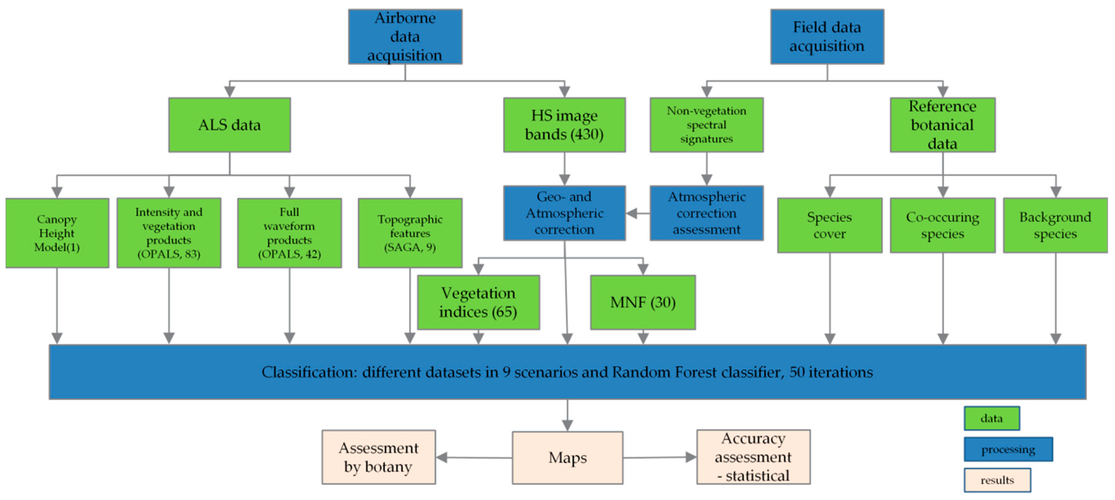
Although in a number of studies, characteristic features of the targeted species such as phenology, colours of flowers, physiological traits and form of growth have been used for their detection, optimal methodologies still remain to be defined. Because the literature lacks the use of hyperspectral with LiDAR data for grassland species identification, this aim remains necessary. Referring to this, the objective of this study is to investigate the use of HySpex data and LiDAR products to classify the two expansive grass species C. epigejos and M. caerulea in Natura 2000 habitats, which have been recognized as aggressive competitors with the tendency of dominating the plant community, causing negative changes in its structure and species composition. More specifically, the investigation aims to:
  • compare different times of airborne data acquisition depending on the growing phase of analysed species, to point out the most optimal time of proper species detection,
  • collate different datasets containing spectral data and additional different vegetation with high layers to choose the most optimal dataset to detect these species.
The presented approach intends to compare these elements with respect to the maximum classification accuracy reached and botanical assessment leading to selecting the most optimal data needed to provide good material for the monitoring of Natura 2000 areas.

2. Data and Methods

2.1. Study Area and Object of the Study

The study area is located in the Silesia Upland in southern Poland under the administrative boundary of Jaworzno town (Figure 1). This part of the town is called Ciężkowice-Pod Łużnikiem (central part of the map) and Ciężkowice (in the northeast part). The vegetation of the study area is a mosaic of planted forest and various types of non-forest plant communities such as grasslands and wet meadows. Our investigations were carried out in non-forest plant communities, mainly wet meadows, still species-rich (southern part of the map) and grassland at the hills in Ciężkowice (eastern part).
In this part of town, a special area of conservation of Nature 2000 habitats “Meadows in Jaworzno” PLH240042 was appointed for the conservation of natural habitats: wet meadows (Molinion) (code: 6410), lowland hay meadows (Arrhenatherion elatioris) (code: 6510) and of species of butterflies: Maculinea (Phengaris) nausithous (code: 6179), and Maculinea (Phengaris) teleius (code: 6177).
As the object of the study two grass species were selected, namely M. caerulea and C. epigejos (Figure 2). Both species belong to native elements in the flora of Poland. They are classified as expansive species and differ in terms of many features, including the type of growth. Expansive species are defined as native species that increase their distribution and colonize new habitats in a geographical area where they are native (they have localities of native occurrence within the same area [70]). According to the definitions accepted for the purpose of this study, native expansive species quickly spread and colonise new areas, in general common plant species, posing a threat as a result of the secondary inheritance for rare plant communities, by often appearing to reduce the biodiversity of natural habitats [71].
M. caerulea (Purple Moor-grass) is a species from the family Poaceae, native to Europe, west Asia, and north Africa. It is an erect, compactly tufted perennial grass, 50–90 cm high, forming either tussocks or extensive swards. Rootstock is more or less creeping, with both stout and fine roots. Leaf blades are flat, 3–8 (max. 10) mm wide, with a bluish-green colour. Panicles are erect, ranking from very dense to open and very loose, dark to light purple, brownish, yellowish, or green with more or less raised branches, 15 cm long. The long narrow purple spikelets are a major identification feature. Fruits have a length of 2 mm. Flowering and fruiting occur in late June or early July to mid-September. Its range of habitats includes wet meadows, heaths, montane grassland, bogs and open woodland. The common features of these habitats, particularly in the area where M. caerulea is found, is permanently or seasonally wet ground. M. caerulea is a very variable species among others owing to variation in overall size, in the length and width of leaves, and especially in the length, width and colour of the panicles. M. caerulea is cultivated for its panicles of purple spikelets on yellow stems [72,73].
C. epigejos (Wood Small-red) is a tall caespitose perennial grass from Poaceae family, widely distributed in, and native to, Eurasia and expanded its range also in North America. The plant forming tufts or tussocks, 60–200 cm, high, with creeping rhizomes. The culms are erect or slightly spreading, usually unbranched. Leaf blades flat, stiff, and hairless, 4–14 (max. 20) mm wide, with dull grey-green colour. Panicles erect, lanceolate to oblong, very dense before and after flowering, 15–30 cm long, 3–6 cm wide, purplish, brownish, or green. Spikelets are densely clustered, narrowly lancelolate or finally gaping. Their fruits have a length of 1 mm. Flowering and fruiting occurs in late June to mid- or late September. Culm height, leaf length, width, shape, and colour are very variable and depend on site factors, especially the light climate or water capacity. Natural habitats supporting C. epigejos include sand dunes, river floodplains, fens, steppes and subalpine grassland but the species is particularly abundant in dry, open grassland that is usually ungrazed, forests, clear cut forest, along railway lines, roadsides and on urban and industrial wasteland. C. epigejos grows on dry, and on flooded soils, but prefers more dry areas than M. caerulea [4,72,73,74]. It is a competitively strong species, which is able to dominate the colonized sites. The plants have two types of clonal growth. The first, intra-vaginal ramet formation, creates groups of closely attached and connected ramets, which we further call ‘‘clumps’’. The other way is formation of extravaginal ramets on rhizomes of several decimeters length [75]. Strong underground rhizomes of C. epigejos can spread up to several meters in one direction, forming dense stands/patches and often caused negative changes in structure and species composition of native plant communities [76,77].

2.2. Remote Sensing Data

Remote sensing data come from instruments that are components of an aerial remote sensing platform, built as part of the HabitARS project by MGGP Aero Company. One of them is the HySpex scanner (Norsk Elektro Optikk, Oslo, Norway), acquiring data with a spatial resolution of 1 m, registered in 470 spectral bands in two ranges of electromagnetic spectrum: Visible and Near Infrared (VNIR, 400–1000 nm) and Shortwave Infrared (SWIR, 930–2500 nm) with 3.26 and 5.45 nm spectral sampling, respectively (Table 1). The sensor has 16-bit radiometric quantization.
The second element of the platform is IGI Lite Mapper 6800 system (Integrated Geospatial Innovations, Kreuztal, Germany), which consists of the Riegl LMS-Q680i Airborne Laser Scanner, from which data was gathered with a point-cloud density of 7 points/m2 (Table 2). Additional component was DigiCAM39 RGB camera (Integrated Geospatial Innovations, Kreuztal, Germany) with 10 cm spatial resolution. Within HabitARS project, the data were acquired in 2016 and 2017. In 2016 it was 21 June, 23 July and 10 September and for 2017 9 June and 11 August. Analyses of data quality allowed for selection of the data from September 2016 and June and August 2017.
A flowchart describing the analysis is shown in Figure 3. It starts from the data acquisition, as the aerial level consisted of ALS and hyperspectral (HS) data, and the field level had botanical data about identified species (see Section 2.3 and was where non-vegetation characteristics measurements were performed. Parallel to aerial data acquisition calibration, spectral curves using ASD FieldSpec 4 spectroradiometer (ASD Inc., Longmont, CO, USA) were collected on 5 polygons for concretes, asphalts and bare grounds in order to validate atmospheric correction of hyperspectral images. Each time 30 samples were collected for each polygon. The images were corrected geometrically using PARGE software [78] (Zurich, Switzerland) and atmospheric correction was performed using ATCOR 4 [79] (Zurich, Switzerland), then the lines were mosaicked. Corrected mosaic was used to classify using original 430 bands as well as for MNF transformation and VIS calculation. The whole image covered 1026 ha area, where 17 ha was occupied by 6410 habitat [80]. Masking of urban land cover based on vector layers with buildings and communication within parcels allowed for removing 137 ha.
Data transformation using MNF was performed for dimensionality reduction selecting the most informative bands [30]. Based on original images covariance matrices were calculated and noise correlations were created, resulting eigenvalues with the highest information (more than 1 value) and the lowest (about zero). From informative curve and experiments with different numbers of bands finally 30 MNF transforms were selected.
Selected MNF transforms were joined with vegetation indices and LiDAR derivatives. Calculation of VIS was performed in ENVI 5.3 software [81] (Broomfield, CO, USA) and 65 indices available using Spectral Indices tool were used, including following vegetation categories: broadband greenness, narrowband greenness, canopy nitrogen, canopy water content, dry or senescent carbon, leaf pigments and light use efficiency.
Processing of LiDAR data consisted of georeferencing, extraction, filtering and classification of point cloud. The point cloud orientation was proceeded using the RiProcess package [82] (Horn, Austria) in Riegl software and the accuracy was assessed at 0.01 cm level of 1 sigma. In 2016, the data were processed into discrete (DISC) type and in 2017 to discrete and additionally to full-waveform (FWF), which provided more information about the targets in the footprint than only location [83]. Full-waveform information was used during postprocessing of raw FWF files to gain more data about vegetation. In order to do this the threshold value was empirically defined (as 3) and used in RiAnalyze software [84] (Horn, Austria). Apart from the threshold, amplitude and pulse width extra byte was used as an additional structural metric for classification, derived using the Riegl RiProcess. The point cloud was classified to ground, noise and vegetation classes using TerraSolid software [85]. Processed point cloud was used to create Canopy Height Model (CHM) and vegetation structure data (Table S1 in Supplementary Materials) in OPALS (Orientation and Processing of Airborne Laser Scanning) software [86] (Vienna, Austria). On the basis of the point cloud, the Digital Terrain Model (DTM) was calculated interpolating points in ground class using moving planes in two iterations. During this process, the following rasters were also calculated: sigmaZ, slope, exposition and Digital Surface Model (DSM), which was calculated by interpolating points from class ground and vegetation (using points with highest z values for each raster cell). The CHM was calculated using a differential model from DSM and DTM created from the ground and vegetation classes. Rasters were calculated on all points with 1 m resolution, classified as ground and classified as vegetation. Finally we calculated 83 discrete rasters that contained different statistics (maximum, minimum, median, mean, range, root mean square, variance) of amplitude, echo ratio and normalized height (Z), exposures, slopes and sigma on Digital Terrain Model and Digital Surface Model, as well as point density and vegetation cover which means the number of returns classified as vegetation divided by the number of all returns multiplied by 100. Full-waveform rasters in the number of 42 contained previously mentioned statistics calculated amplitude and pulse width, and also for all points, ground and vegetation. Topographic indexes (TOPO) were also generated using Terrain analysis package of SAGA software [87] (Hamburg, Germany) and they were: Topographic Position Index, Topographic Wetness Index, Direct Insolation, Slope, Aspect, Module Multiresolution Index of Valley Bottom Flatness, Multi-resolution Ridge Top Flatness and Modified Catchment Area.
Selected MNF bands were combined with calculated indices and LiDAR derivatives in ENVI using Layer Stacking. The datasets were called scenarios, with corresponding number listed in Table 3. The dataset consisting original mosaic of spectral bands called sc01 was also created to check if the original or transformed data will perform better, which is important from an operational point of view.

2.3. Reference Botanical Data

Simultaneously with the acquisition of airborne data, on-ground botanical reference data were obtained three times during the growing season (spring, summer and autumn) with the purpose of assessing the species detection possibilities at different phases of the life cycle, on research areas (of average size 5 km2), where these species occurred at diverse frequencies and cover. The data collected were used to identify species characteristics such as percentage cover in reference polygons, growth stage, flowering and fruiting stage, discoloration/damage, list of co-occurring species in particular that have cover above 20%, and additional information, i.e., % of bare ground, % of vegetation, % of mosses and % of litter (necromass) and type of land use (mowing, pasturage). For each of the plant species analysed, at least 100 reference 2-m buffer polygons (Table 4, Figure 4) were gathered together with a similar number of reference polygons for surrounding vegetation or other species with similar morphology or with frequently coexisting species (e.g., Solidago canadensis and S. gigantea). These polygons were treated as a “background” class, which were reference 2-m buffer polygons, established in the patch of the species not chosen regarding the invasion/expansion in the plant community, provided that an examined species is not acting in it or covering it doesn’t exceed the 10%. All data were stored in GNSS receiver Spectra Precision GPS MobileMapper 120 (Spectra Geospatial, Westminster, CA, USA) and in traditional field data form and finally in the database. Additionally, to the database were joined polygons of “background” class drawn manually based on orthophotomaps from RGB camera, referred to as “forest” and “shadow” (in the number of 30 per class).
The first step of validation of reference data was assessing the correctness of polygons which means the removing of shadowed or mowed polygons of species. These types of errors could be caused by collecting ground botanical data few days after aerial data acquisition. The next step of preparing the reference data was an analysis of mistakes and errors. The aim of this stage was to capture errors from the database related to the incorrect entry of the name of the site by the botanical team during field measurements or the recognition of the site, where there are species strongly related to other classes—also mistakes from the field. This kind of error could not be discovered in the early steps. Based on a t-distributed stochastic neighbour embedding (t-SNE) machine learning algorithm, the most spectrally homogeneous groups of polygons without errors were selected [88]. It is a non-linear data size reduction technique that simplifies multi-dimensional space down to two or three dimensions. The analysis was performed on the basis of 30 MNF bands in R software [89]. In this way, the similarity of reference sites between classes was determined on the basis of remote sensing data. On the basis of analysis of the botanical database, outliers were determined by botanists, which should be removed from further analyses. As a result, 14 errors were found in polygons gathered in September 2016 for C. epigejos. Finally, for evaluating the performance of the classification method, the ratio of the total area of used reference data collected to the study site area (excluding mask of urban land cover) was calculated and it was the following: 0.001973 for both M. caerulea and C. epigejos classification in June; 0.002186 for M. caerulea and 0.002175 for C. epigejos in August and 0.001994 for M. caerulea and 0.001948 for C. epigejos in September.

2.4. Random Forest Classification and Accuracy Assessment

To acquire information about the best dataset and time of data the Random Forest decision tree ensemble classifier [90] was used. In each classification two parameters were used: ntree (number of trees) equal to 100 and mtry (number of features randomly sampled as candidates at each split) equal sqrt (n_features), where n_features was the number of used layers in the classification. The mtry value was set as a default value and also to make it possible to analyse all features in each tree [37]. This was done separately for C. epigejos and M. caerulea—in each classification two classes were classified (species and background). To make the information more objective, the classification was performed 50 times for each dataset and campaign. The field data were randomly sampled using 50/50% of training and validation split. Based on the previous experiments only species with greater than 40% covered in polygons were chosen as study objects.
The results for single classification and set of classifications were compared based on the Kappa statistic [91,92] which is the common method of evaluation in machine learning classification problems [37,93]. The nonparametric U Mann-Whitney-Wilcoxon test was used to evaluate the statistical significance of the differences in Kappa accuracy between classifications with different scenarios. Significant differences between the groups were assessed at p = 0.05. The user (UA) and producer (PA) accuracies for species and background were calculated and then the weighted mean of both values as F1 statistics were combined [94]. For the best Kappa values in each classification set, the maps of species distribution were produced, and the confusion matrix was analysed.

3. Results

The results were presented on the maps (Figure 5) and calculated accuracies (Figure 6 and Figure 7).
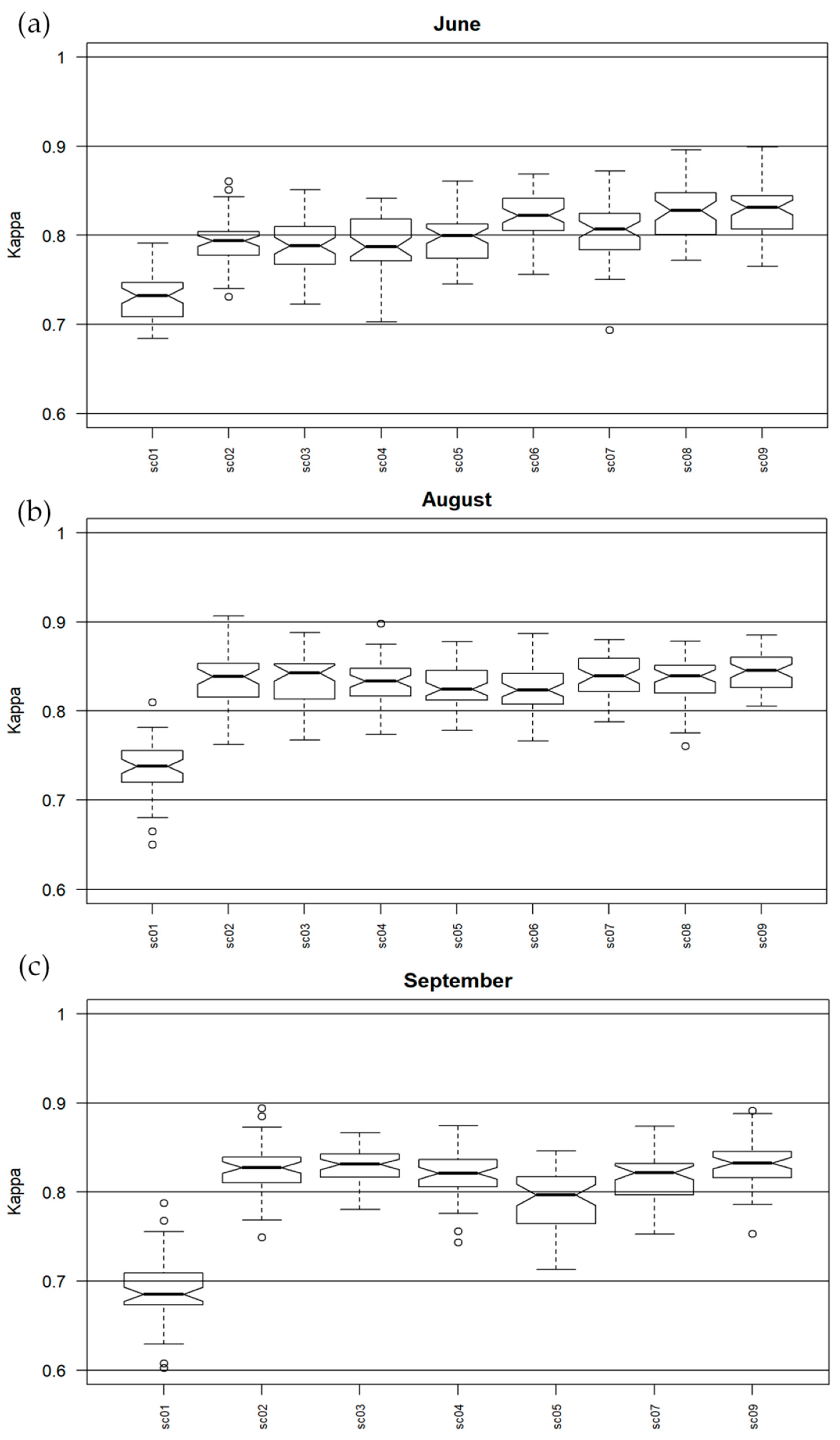
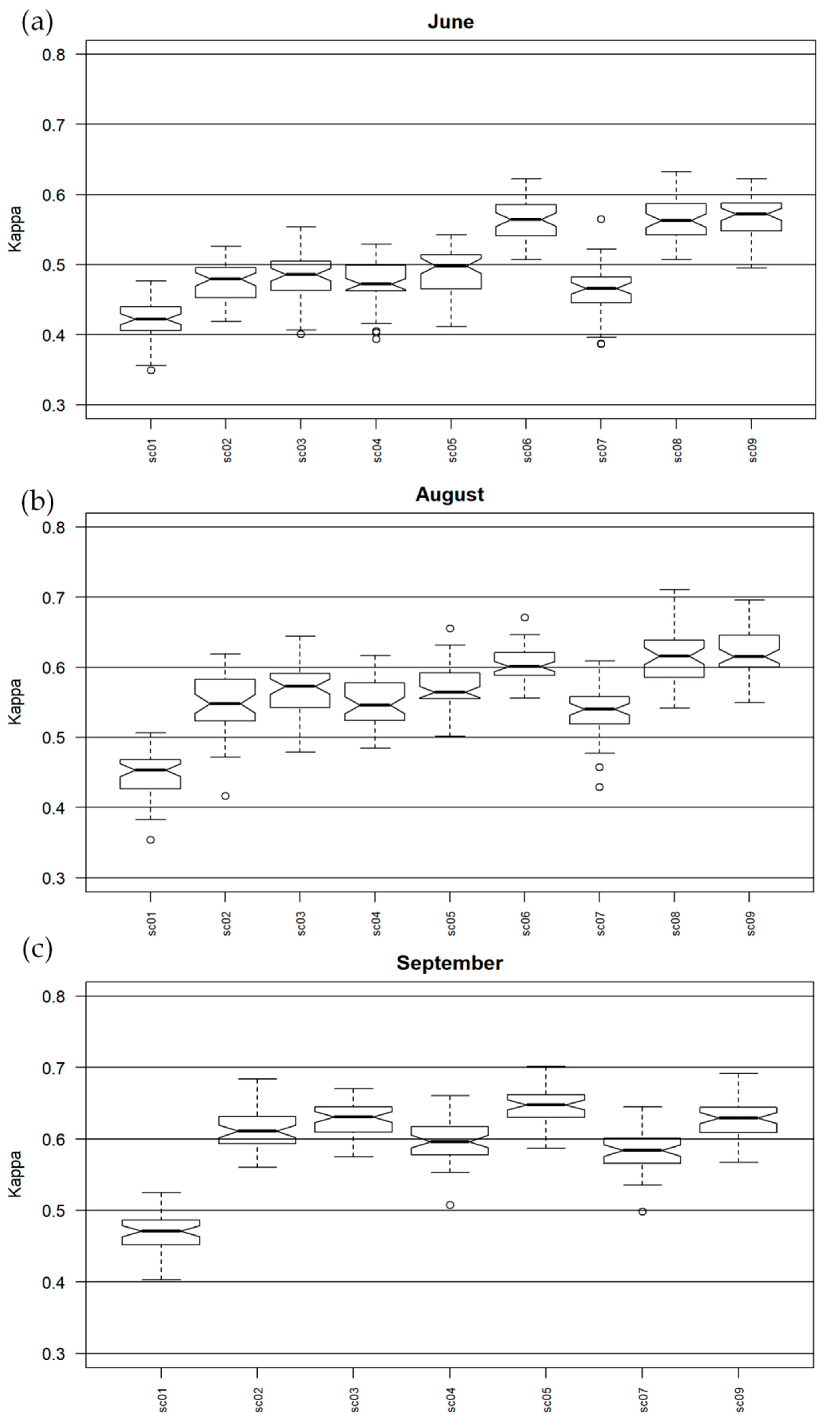
The Kappa accuracy obtained for the classification in each campaign was presented in boxplots. Datasets for differences that were not statistically significant were listed in 
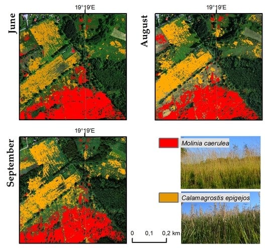
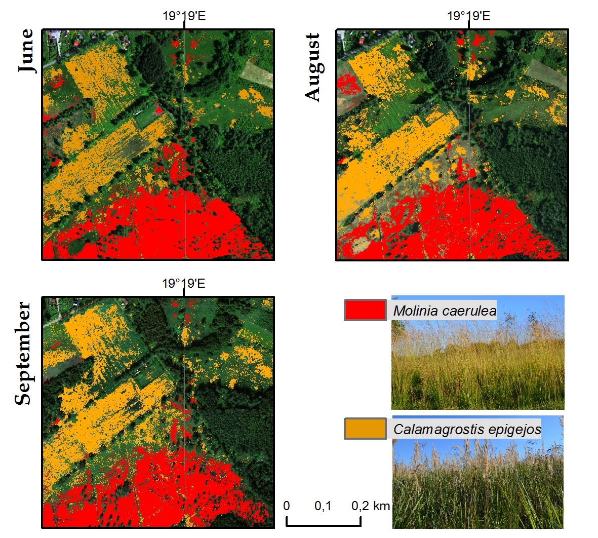
Table S2 in Supplementary Materials. Because sc01 contains a mosaic of all spectral bands, the differences between it and the other scenarios in which MNF channels were used are significant. For Molinia in June, the highest Kappa accuracy (around 0.83) was obtained for a group of sets that used MNF transforms and full-waveform products from LiDAR, as well as for MNF with all additional layers (sc09), a slightly lower accuracy for pairs: MNF + topographic indexes and MNF + discrete data from LiDAR (approx. 0.81). For the group in which the MNF alone and MNF bands with VIS and CHM were used, the Kappa median value was lower (0.79) and these scenarios presented the most diversified values obtained during 50 iterations. In August, the accuracy for Molinia was more stable and reached the highest level. Aside from sc01, all medians were higher than 0.8. The best set included MNF with topographic indices and full-waveform data; in contrast, the lowest level of dispersion of results was obtained for all additional layers from MNF (sc09). The scenario containing the MNF bands alone was not statistically different from other MNF scenarios, but it had the highest level of dispersion. In September, the differences between data sets for Molinia were much higher than in August. The highest accuracy was obtained for MNF, MNF + CHM and MNF with all additional layers, but the lowest level of dispersion was observed for sc03. A pair of data sets with discrete data of the lowest values and the highest level of value dispersion stand out in particular. For sc01, the Kappa median was the lowest (0.69).
Accuracy for species and background was also calculated for the result obtained during the best iteration. It was a combination of producer and user accuracy, which is referred to as the F1 value. For M. caerulea (Table 5), this accuracy confirms the accuracy of Kappa—the lowest values were obtained for June. The best dataset in June was sc08, where F1 reached 0.87; the lowest value was for sc01 (0.72). In general, F1 accuracies were the best in August, most of the median values for scenarios was 0.86, the highest was 0.89 for sc09 and even sc01 consisted of mosaic of spectral data was also high and reached a 0.84 value. September was the second highest in term of class accuracies and here the best was also sc09 with 0.88 value, next was sc04 and 05 with 0.87 value. A slightly lower value for sc08 (0.82) was noticeable.
For C. epigejos in June the median of Kappa values were between 0.4 and 0.6 and the highest were for MNF transforms with full-waveform and discrete LiDAR rasters therefore also for all rasters in sc09. Also mosaic of spectral bands and MNF with topographic indexes presented the worst results. A similar situation applied for August, but the accuracies were slightly higher for each dataset, while the highest median values were for sc08 and sc09 but the lowest level of dispersion was for MNF with discrete and full-waveform LiDAR data. For September, the values were the most stable and also the best dataset contained discrete LiDAR data. In each campaign, information on the intensity and structure of vegetation for C. epigejos was essential and improved accuracy. For July and August, the highest accuracy was obtained for full-waveform data; in September, due to the lack of full-waveform data, the highest accuracy was obtained for discrete data.
F1 values for C. epigejos also confirm Kappa accuracies for each campaign and dataset (Table 6). The lowest values were for June, where the best dataset was sc09 (0.67%), the worst sc01 (0.54%) but sc03 was similar (0.56%). The same situation was observed for August, but here the values were slightly higher, in general: the best was sc09 (0.7) and the worst sc01 (0.6) and sc02 (0.61). C. epigejos was classified most correctly in September; however, sc05 turned out to be the best set here.

4. Discussion

Based on Landis et al. [95] values between 0.61 and 0.80 indicate substantial strength of the agreement, while more than 0.81 means almost perfect agreement of the classification. Based on this information, it can be concluded that M. caerulea was classified very well in each date and almost each scenario. In the case of Kappa accuracy for the entire image and F1 accuracy for individual classes, adding information about the vegetation structure from LiDAR improved the results. The difference between the use of discrete and full-waveform data was small but noticeable, which allows for the conclusion to be drawn that newer full-waveform technology that derived amplitude and used pulse width extra byte performed better. Adding this information to the September data could improve accuracy.
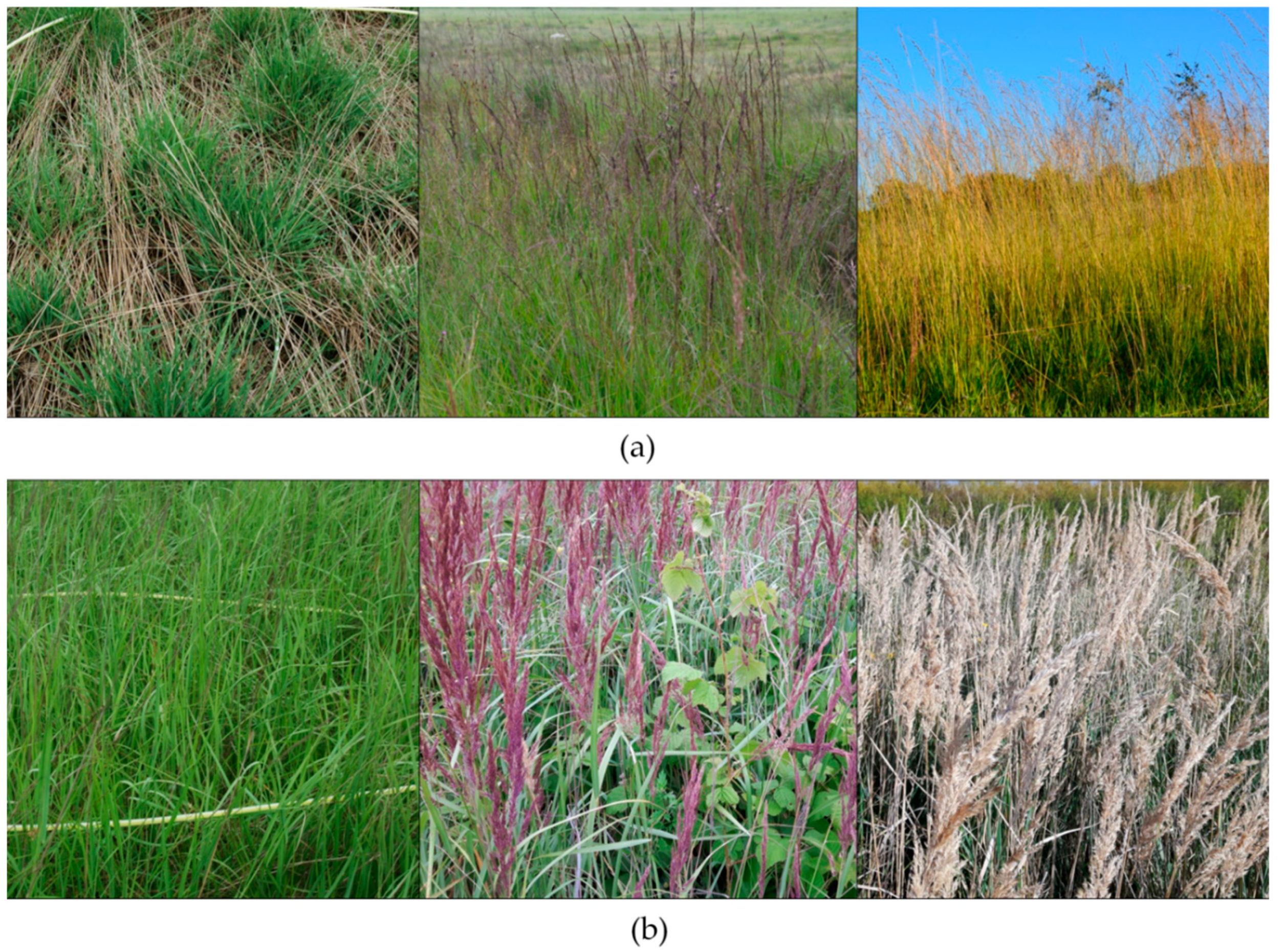
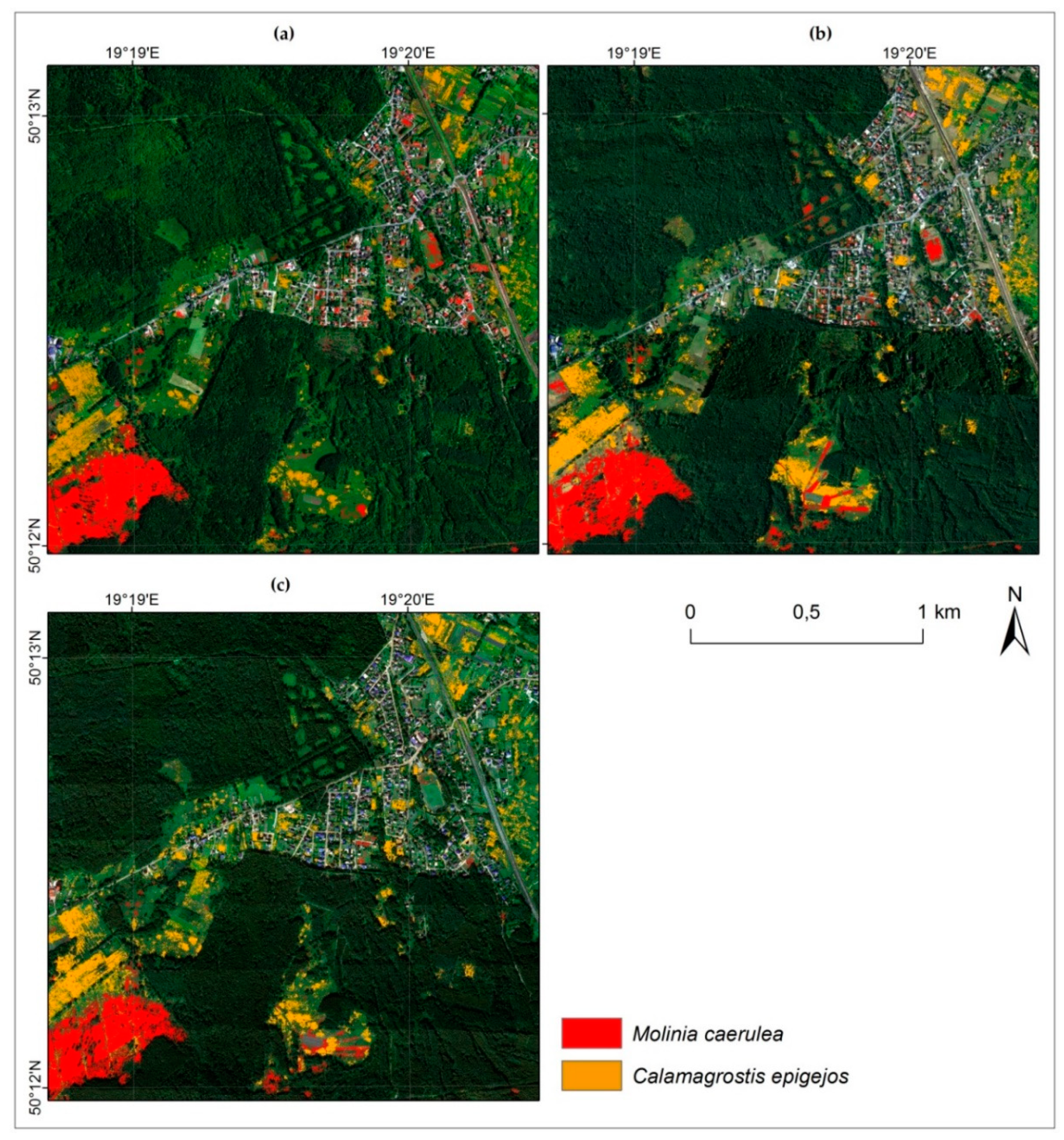
Referring to the visual interpretation and botanical evaluation, Molinia is best detectable in the flowering phase, which occurs between July and September, but reaches its peak in August. It should be noted that the coverage of most sites with the Molinia species was high at that time (70%–80%) and the co-existence of other species was rare. However, there was occasional overestimation of the species, especially for the results of August and September, with some artefacts, e.g., pathways to the south of the site, being classified as species.
The usefulness of only spectral information to discrimination of M. caerulea is supported by other studies [20,68]. In classification of Natura 2000 heathlands in Kalmthoutse Heide in Belgium [69] the best mean accuracies were obtained for heathlands with Molinia (80.7% using SVM classifier, 69.7% using RF) on CHRIS data from July. Marcinkowska-Ochtyra et al. [20] presented M. cearulea community classification in Giant Mountains in Poland/Czech Republic with 90.3% of PA with APEX data from September using SVM. However, the assumption of these analyses were not to compare different growing stages of the species and were conducted on the data acquired once, but in each case Molinia was well classified. In other Natura 2000 heathlands area, Dutch Ederheide and Ginkelse heide [46], M. caerulea encroachment abundance was estimated using AHS-160 (Airborne Hyperspectral Scanner) and Spectral Mixture Analysis (SMA) showing the correlation with field estimates at 0.48 R2 value. The authors pointed out that time of acquisition (October) was unsuitable and did not allow for distinguishing Deschampsia flexuosa from M. caerulea. Molinion caeruleae was one of the best classified plant association in grassland habitats classification in Döberitzer Heide, west Berlin, reaching 96% of F1 accuracy due to a dominant yellow colour in autumn on RapidEye data and the fact that its flowering phase is later than for any other species [33]. In the study presented here it should be noticed that last date of acquisition of airborne data was the beginning of September and M. caerulea were not changing colour into yellow yet, so according to Schuster et al. [33] the accuracies could be much better when data would be collected near to the end of September. High accuracy was for intra-annual time series of RapidEye and TerraSAR-X [33], so adding vegetation structure information from radar data was useful. In grasslands classification based on only LiDAR full-waveform data in the Natura 2000 site in Sopron, Hungary [54], M. caerulea reached UA and PA between 60% and 80%, the authors found it overestimated but this was caused by the flight strip edges on Echo Width. Comparative tests performed in the frame of study presented here used only LiDAR data for M. caerulea classification [96]. In the first test full-waveform data were used for the best classified date (August) obtained previously and median Kappa from 5 iterations of calculated accuracies were 42.7% and F1 equal to 47.4% (PA and UA between 35%–74%). The second test was based on using only discrete data for September and it allowed us to reach 32.7% median Kappa and 34% median F1 (PA and UA between 25%–77%). Because the differences between used datasets with MNF transforms and tested here are significant, it underlines the importance of spectral information in discrimination of the species. This view is supported by Debes et al. [64] and Luo et. al [65], where improving the accuracy and efficiency of LiDAR applications after incorporation of passive optical remote sensing data were observed.
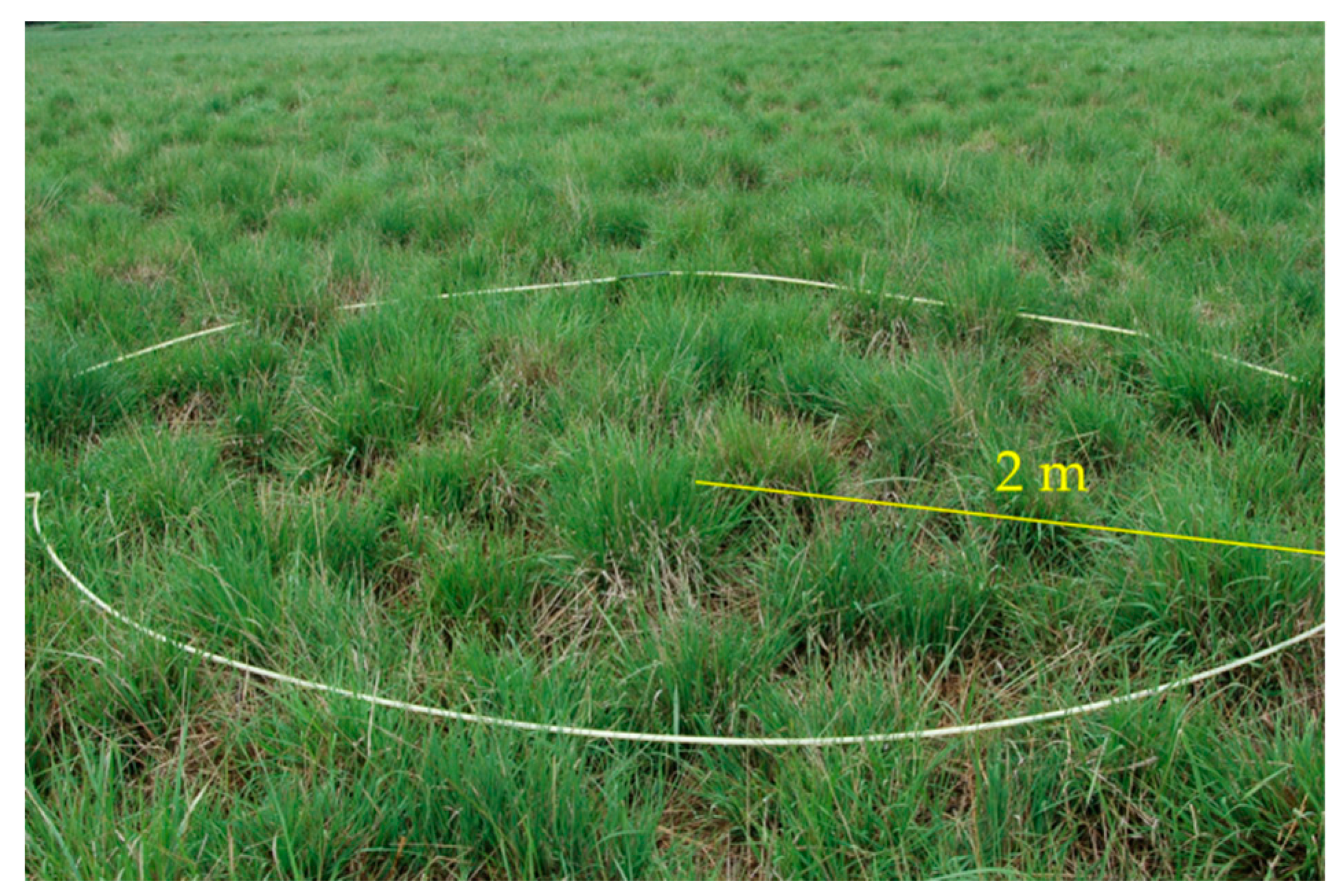
The result achieved in these examinations corresponds to the actual state of affairs, confirmed in traditional field research. Because of training and validation, only greater than 40% species cover in polygon patches with cover of M. caerulea lower than 30% were poorly detected, but one should take in mind that the species is a characteristic component of native vegetation (characteristic species for plant communities of Molinion caeruleae wet meadows). From the point of view of needs of protection of these habitats involving increasing the covering of this species, exceeding the 50% level, which can indicate about progressing disadvantageous changes, is significant.
The range for Kappa values for C. epigejos could be interpreted as moderate in June [95] for all scenarios and in August for all except sc08 and 09, to substantial in September, excluding sc01 and MNF with topographic indexes. For both Kappa and F1 values for this species, an increase in accuracy was observed using discrete and full-waveform data derived from LiDAR, which confirms that adding detailed information on the height and structure of vegetation is crucial in distinguishing these species from their background. Worse accuracy results were also noticeable for MNF and MNF with topographic indices in each campaign, which confirms the expansive nature of this species.
C. epigejos blooms from June to August and is in the fruiting phase in September. In the botanical evaluation of the results, the distribution of the species is fairly well presented due to the peak phase of fruiting. In this case, Calamagrostis coverage of over 60% is well-detectable. The main co-existing species is Solidago spp., which blooms and fruits at a similar time as the C. epigejos but differs in colour and shape. However, since these two species mingle with each other, it is often difficult to identify each of them within a pixel with a resolution of 1 m.
In general, species of the genus Calamagrostis belong to the group of species that is difficult to identify with remote sensing techniques. It is supported by unpublished analysis of C. epigejos classified on September collections of HySpex data on two other Natura 2000 sites in Poland [97], where Kappa accuracies were between 50%–60% and F1 between 60%–65%, influenced also by local conditions. Comparative test with using only discrete LiDAR data for C. epigejos classification in Jaworzno Meadows were also conducted [96], giving the median Kappa accuracies of about 18% and a median F1 value equal to 31% (UA and PA between 22%–52%). As in M. caerulea test, this analysis showed that for discrimination of C. epigejos the best method was the combination of spectral and height-dependent variables. However, higher accuracies were obtained using only hyperspectral data [19,20,98]. In [19,20] the authors found out that a plant community with Calamagrostis villosa in subalpine part of Giant Mountains classified on APEX data from September at about 70% level of PA. They observed this species encroaching into lower parts of the upper forest border. A similar situation was detected in Tatra vegetation classification on DAIS, with 7915 hyperspectral data acquired in August when the Calamagrostietum villosae community reached one of the most diverse results and the accuracy was also about 70% [98]. These analyses were carried out at the level of plant communities; therefore, it should be noted that it is the species that is being classified, which requires a slightly different approach. Both areas in mentioned literature were located in high mountains, where the variation of local conditions are totally different to in the lowlands. In the literature there is lack of detailed studies on the classification of the species C. epigejos, so the work presented here is the beginning of a discussion for further research.
Comparing both species’ classification results, the accuracies obtained for C. epigejos were worse than for M. caerulea. The reason for this is probably that C. epigejos has a wider ecological spectrum and is appearing in analysed areas in various habitat conditions—from humid to dry and with the diversified cover, and is co-occurring with a substantial amount of species with which it can be confused.
When transferring the method to other areas, ground data with specific characteristics should be collected (more than 40 percentage of species cover, information about co-occurring species, especially these visually similar to analysed species), as well as the best time of acquisition for individual species connected with growing season should be kept in mind. The basis of dataset is hyperspectral mosaic transformed using dimensionality reduction method as MNF. Analysing the date of acquisition where grassland species differ considerably from the background requires LiDAR products, especially full-waveform or discrete rasters to improve the accuracy levels. For the hazard assessment created by expansive species the method presented in this study is bringing expected results and can be recommended for supporting traditional botanical field methods.

5. Conclusions

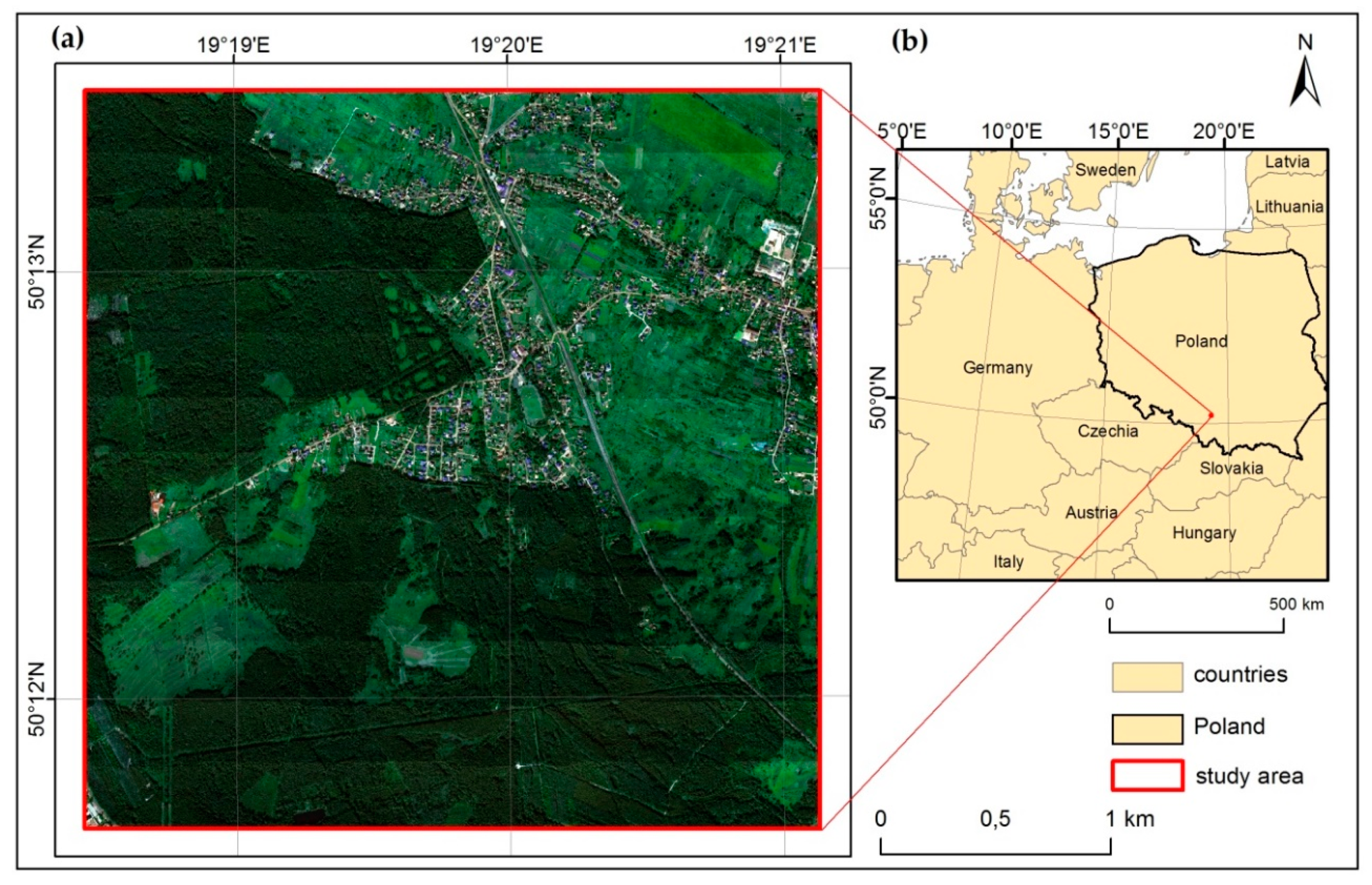
The expansive species encroachment into non-forest habitats under protection is a very important ecological task and it should be monitored. This study investigated the use of HySpex and LiDAR data for mapping the distribution of M. caerulea and C. epigejos—expansive grass species in “Jaworzno Meadows” Natura 2000 site in Poland at their different growth stages. The species were classified using a Random Forest algorithm with 7–9 scenarios of different datasets consisting of spectral data, MNF transforms and MNF with LiDAR derivatives. The Kappa accuracy assessment was performed iteratively using 50 repetitions of procedure, giving more objective results obtained for the different scenarios on data collected for three months. Additionally, for the best results, F1 accuracies for species and background class were calculated. In each case the dataset containing original spectral bands was the worst comparing to MNF transformation, only the F1 value for M. caerulea was slightly higher. In most cases the best dataset was sc09, consisting of MNF with all calculated LiDAR derivatives, but from an operational point of view, it is not the optimal solution. Adding intensity and vegetation structure data from LiDAR improved the results, especially full-waveform data from 2017 because of the more detailed information registered. The results show the worst accuracies obtained for the original data consisted of spectral bands.
M. caerulea spectral characteristics with used data allowed for better recognition than C. epigejos, which co-occurs with greater number of other species. Especially for C. epigejos classification datasets with topographic indexes worse accuracies were observed, which confirms the expansive character of the species, as it prefers wet and dry habitats. For M. caerulea it was not observed, confirming the preference of wetter areas. Predominantly the datasets with MNF and additional CHM or vegetation indexes did not show the differences to be significant statistically. The correctness of the result was influenced by the species covering in the polygon (the highest at the time of full flowering/fruiting), the maximum biomass and co-existing of other species. The best time to identify C. epigejos was September (optimum fruit formation) and for M. caerulea was August. The flowering period of the species was the recommended time to detect the species because of the high cover of the species in polygons (80%–100%).
The next step of this research could be feature selection giving the information which features from whole dataset allowed for the best classification results and then selecting only these to further analysis. It could make the procedure of species identification even more operational. However, our results are valuable because they show the potential of each dataset used, which is repeated three times, allowing for mapping of each species with relatively high accuracy. The results provide analytical potential for expansive species studies and great support for field work.

Supplementary Materials

The following are available online at https://0-www-mdpi-com.brum.beds.ac.uk/2072-4292/10/12/2019/s1, Table S1: Vegetation structure rasters used in the study, Table S2. Datasets for which Kappa accuracy differences were not significant statistically using U Mann-Whitney-Wilcoxon test.

Author Contributions

A.M.-O. and A.J. conceptualized the manuscript and design the methodology. A.M.-O. performed the experiment and results analysis, wrote original draft of the manuscript and prepared the figures. K.B. and B.T.-G. wrote Section 2.1 and Section 2.3, collected field data and help with results analysis. All of authors read and revised the manuscript.

Funding

Research has been carried out under the Biostrateg Programme of the Polish National Centre for Research and Development (NCBiR), project DZP/BIOSTRATEG-II/390/2015: The innovative approach supporting monitoring of non-forest Natura 2000 habitats, using remote sensing methods (HabitARS).

Acknowledgments

We wish to express our sincere gratitude to the whole Consortium for work in HabitARS project, especially to MGGP Aero Company for acquiring and pre-processing aerial data, Warsaw University of Life Sciences and University of Lodz for joining us in defining the concept of species classification as part of the WP6 task, to Warsaw University of Technology for processing of LiDAR data, to Adam Kania for technical support with classification and similarity analysis and Edwin Raczko for help with statistical analyses.

Conflicts of Interest

The authors declare no conflict of interest.

References

  1. Hooftman, D.A.P.; Bullock, J.M. Mapping to inform conservation: A case study of changes in semi-natural habitats and their connectivity over 70 years. Biol. Conserv. 2012, 145, 30–38. [Google Scholar] [CrossRef]
  2. Wesche, K.; Krause, B.; Culmsee, H.; Leuschner, C. Fifty years of change in Central European grassland vegetation: Large losses in species-richness and animal-pollinated plants. Biol. Conserv. 2012, 150, 76–85. [Google Scholar] [CrossRef]
  3. Krause, B.; Culmsee, H. The significance of habitat continuity and current management on the compositional and functional diversity of grasslands in the uplands of Lower Saxony, Germany. Flora 2013, 208, 299–311. [Google Scholar] [CrossRef]
  4. Rebele, F.; Lehmann, C. Biological Flora of Central Europe: Calamagrostis epigejos (L.) Roth. Flora 2001, 196, 325–344. [Google Scholar] [CrossRef]
  5. Hejcman, M.; Češková, M.; Pavlů, V. Control of Molinia caerulea by cutting management on sub-alpine grassland. Flora Morphol. Distrib. Funct. Ecol. Plants 2010, 205, 577–582. [Google Scholar] [CrossRef]
  6. Holub, P.; Tůma, I.; Záhora, J.; Fiala, K. Different nutrient use strategies of expansive grasses Calamagrostis epigejos and Arrhenatherum elatius. Biologia 2012, 67, 673–680. [Google Scholar] [CrossRef]
  7. Pruchniewicz, D.; Donath, T.W.; Otte, A.; Żołnierz, L.; Eckstein, R.L. Effect of expansive species on seed rain and soil seed bank of mountain mesic meadows. Tuexenia 2016, 36, 81–96. [Google Scholar]
  8. Dorigo, W.; Lucieer, A.; Podobnikar, T.; Čarni, A. Mapping invasive Fallopia japonica by combined spectral, spatial, and temporal analysis of digital orthophotos. Int. J. Appl. Earth Obs. Geoinf. 2012, 19, 185–195. [Google Scholar] [CrossRef]
  9. Bradley, B.A. Remote detection of invasive plants: A review of spectral, textural and phenological approaches. Biol. Invasions 2014, 16, 1411–1425. [Google Scholar] [CrossRef]
  10. Müllerová, J.; Brůna, J.; Bartaloš, T.; Dvořák, P.; Vítková, M.; Pyšek, P. Timing Is Important: Unmanned Aircraft vs. Satellite Imagery in Plant Invasion Monitoring. Front. Plant Sci. 2017, 8, 887. [Google Scholar] [CrossRef]
  11. Huang, C.Y.; Asner, G.P. Applications of remote sensing to alien invasive plant studies. Sensors 2009, 9, 4869–4889. [Google Scholar] [CrossRef] [PubMed]
  12. Zlinszky, A.; Kania, A. Will it blend? Visualization and accuracy evaluation of high-resolution fuzzy vegetation maps. Int. Arch. Photogramm. Remote Sens. Spat. Inf. Sci. 2016, XLI-B2, 335–343. [Google Scholar] [CrossRef]
  13. Gao, B.C. NDWI—A normalized difference water index for remote sensing of vegetation liquid water from space. Remote Sens. Environ. 1996, 58, 257–266. [Google Scholar] [CrossRef]
  14. Goward, S.N.; Markham, B.; Dye, D.G.; Dulaney, W.; Yang, J. Normalized difference vegetation index measurements from the Advanced Very High Resolution Radiometer. Remote Sens. Environ. 1991, 35, 257–277. [Google Scholar] [CrossRef]
  15. Wang, L.; Qu, J.J. NMDI: A normalized multi-band drought index for monitoring soil and vegetation moisture with satellite remote sensing. Geoph. Res. Lett. 2007, 34. [Google Scholar] [CrossRef]
  16. Kycko, M.; Zagajewski, B.; Lavender, S.; Romanowska, E.; Zwijacz–Kozica, M. The Impact of Tourist Traffic on the Condition and Cell Structures of Alpine Swards. Remote Sens. 2018, 10, 220. [Google Scholar] [CrossRef]
  17. Zagajewski, B.; Tømmervik, H.; Bjerke, J.W.; Raczko, E.; Bochenek, Z.; Kłos, A.; Jarocińska, A.; Lavender, S.; Ziółkowski, D. Intraspecific Differences in Spectral Reflectance Curves as Indicators of Reduced Vitality in High–Arctic Plants. Remote Sens. 2017, 9, 1289. [Google Scholar] [CrossRef]
  18. Hamada, Y.; Stow, D.A.; Coulter, L.L.; Jafolla, J.C.; Hendricks, L.W. Detecting Tamarisk species (Tamarix spp.) in riparian habitats of Southern California using high spatial resolution hyperspectral imagery. Remote Sens. Environ. 2007, 109, 237–248. [Google Scholar] [CrossRef]
  19. Marcinkowska–Ochtyra, A.; Zagajewski, B.; Ochtyra, A.; Jarocińska, A.; Wojtuń, B.; Rogass, C.; Mielke, C.; Lavender, S. Subalpine and alpine vegetation classification based on hyperspectral APEX and simulated EnMAP images. Int. J. Remote Sens. 2017, 38, 1839–1864. [Google Scholar] [CrossRef]
  20. Marcinkowska–Ochtyra, A.; Zagajewski, B.; Raczko, E.; Ochtyra, A.; Jarocińska, A. Classification of High-Mountain Vegetation Communities within a Diverse Giant Mountains Ecosystem Using Airborne APEX Hyperspectral Imagery. Remote Sens. 2018, 10, 570. [Google Scholar] [CrossRef]
  21. Jensen, J.R. Biophysical remote sensing. Ann. Assoc. Am. Geogr. 1983, 73, 111–132. [Google Scholar] [CrossRef]
  22. Carrão, H.; Gonçalves, P.; Caetano, M. Contribution of multispectral and multitemporal information from MODIS images to land cover classification. Remote Sens. Environ. 2008, 112, 986–997. [Google Scholar] [CrossRef]
  23. Schneider, J.; Grosse, G.; Wagner, D. Land cover classification of tundra environments in the Arctic Lena Delta based on Landsat 7 ETM+ data and its application for upscaling of methane emissions. Remote Sens. Environ. 2009, 113, 380–391. [Google Scholar] [CrossRef] [Green Version]
  24. Golenia, M.; Zagajewski, B.; Ochtyra, A.; Hościło, A. Semiautomatic land cover mapping according to the 2nd level of the CORINE Land Cover legend. Pol. Cartog. Rev. 2015, 47, 203–212. [Google Scholar] [CrossRef] [Green Version]
  25. Riaño, D.; Chuvieco, E.; Salas, J.; Aguado, I. Assessment of different topographic corrections in Landsat–TM data for mapping vegetation types. IEEE Trans. Geosci. Remote Sens. 2003, 41, 1056–1061. [Google Scholar] [CrossRef]
  26. Jędrych, M.; Zagajewski, B.; Marcinkowska–Ochtyra, A. Application of Sentinel–2 and EnMAP new satellite data to the mapping of alpine vegetation of the Karkonosze Mountains. Pol. Cartog. Rev. 2017, 49, 107–119. [Google Scholar] [CrossRef]
  27. Chan, J.C.W.; Spanhove, T.; Ma, J.; Borre, J.V.; Paelinckx, D.; Canters, F. Natura 2000 Habitat Identification and Conservation Status Assessment with Superresolution Enhanced Hyperspectral (CHRIS/Proba) Imagery. In Proceedings of the GEOBIA 2010 Geographic Object-Based Image Analysis, Ghent, Belgium, 29 June–2 July 2010. [Google Scholar]
  28. Goetz, A.F.H.; Vane, G.; Solomon, J.E.; Rock, B.N. Imaging spectroscopy for earth remote sensing. Science 1985, 228, 1147–1153. [Google Scholar] [CrossRef]
  29. Hotelling, H. Analysis of a complex of statistical variables into principal components. J. Educ. Psychol. 1933, 24, 417–441. [Google Scholar] [CrossRef]
  30. Green, A.A.; Berman, M.; Switzer, P.; Craig, M.D. A transformation for ordering multispectral data in terms of image quality with implications for noise removal. IEEE Trans. Geosci. Remote Sens. 1988, 26, 65–74. [Google Scholar] [CrossRef] [Green Version]
  31. Xie, Y.; Sha, Z.; Yu, M. Remote sensing imagery in vegetation mapping: A review. J. Plant Ecol. 2008, 1, 9–23. [Google Scholar] [CrossRef]
  32. Geerken, R.; Zaitchik, B.; Evans, J.P. Classifying rangeland vegetation type and coverage from NDVI time series using Fourier Filtered Cycle Similarity. Int. J. Remote Sens. 2005, 26, 5535–5554. [Google Scholar] [CrossRef] [Green Version]
  33. Schuster, C.; Schmidt, T.; Conrad, C.; Kleinschmit, B.; Förster, M. Grassland habitat mapping by intra-annual time series analysis–Comparison of RapidEye and TerraSAR-X satellite data. Int. J. Appl. Earth Obs. Geoinf. 2015, 34, 25–34. [Google Scholar] [CrossRef]
  34. Zhang, C.; Xie, Z. Object-based vegetation mapping in the Kissimmee River watershed using HyMap data and machine learning techniques. Wetlands 2013, 33, 233–244. [Google Scholar] [CrossRef]
  35. Burai, P.; Deák, B.; Valkó, O.; Tomor, T. Classification of herbaceous vegetation using airborne hyperspectral imagery. Remote Sens. 2015, 7, 2046–2066. [Google Scholar] [CrossRef]
  36. Lawrence, R.L.; Wood, S.D.; Sheley, R.L. Mapping invasive plants using hyperspectral imagery and Breiman Cutler classifications (RandomForest). Remote Sens. Environ. 2006, 100, 356–362. [Google Scholar] [CrossRef]
  37. Cutler, D.R.; Edwards, T.C., Jr.; Beard, K.H.; Cutler, A.; Hess, K.T.; Gibson, J.; Lawler, J.J. Random forests for classification in ecology. Ecology 2007, 88, 2783–2792. [Google Scholar] [CrossRef] [PubMed]
  38. Naidoo, L.; Cho, M.A.; Mathieu, R.; Asner, G. Classification of savanna tree species, in the Greater Kruger National Park region, by integrating hyperspectral and LiDAR data in a Random Forest data mining environment. ISPRS J. Photogramm. Remote Sens. 2012, 69, 167–179. [Google Scholar] [CrossRef]
  39. Ghosh, A.; Fassnacht, F.E.; Joshi, P.K.; Koch, B. A framework for mapping tree species combining hyperspectral and LiDAR data: Role of selected classifiers and sensor across three spatial scales. Int. J. Appl. Earth Obs. Geoinf. 2014, 26, 49–63. [Google Scholar] [CrossRef]
  40. Raczko, E.; Zagajewski, B. Comparison of Support Vector Machine, Random Forest and Neural Network Classifiers for Tree Species Classification on Airborne Hyperspectral APEX images. Eur. J. Remote Sens. 2017, 50, 144–154. [Google Scholar] [CrossRef]
  41. Ustin, S.L.; DiPietro, D.; Olmstead, K.; Underwood, E.; Scheer, G.J. Hyperspectral Remote Sensing for Invasive Species Detection and Mapping. In Proceedings of the 2002 IEEE International Geoscience and Remote Sensing Symposium, Toronto, ON, Canada, 24–28 June 2002. [Google Scholar]
  42. Pengra, B.W.; Johnston, C.A.; Loveland, T.R. Mapping an invasive plant, Phragmites australis, in coastal wetlands using the EO–1 Hyperion hyperspectral sensor. Remote Sens. Environ. 2007, 108, 74–81. [Google Scholar] [CrossRef]
  43. Asner, G.P.; Jones, M.O.; Martin, R.E.; Knapp, D.E.; Hughes, R.F. Remote sensing of native and invasive species in Hawaiian forests. Remote Sens. Environ. 2008, 112, 1912–1926. [Google Scholar] [CrossRef]
  44. Házi, J.; Bartha, S.; Szentes, S.; Wichmann, B.; Penksza, K. Seminatural grassland management by mowing of Calamagrostis epigejos in Hungary. Hung. Acad. Sci. 2011, 145, 699–707. [Google Scholar] [CrossRef]
  45. Jacquemyn, H.; Brys, R.; Neubert, M.G. Fire increases invasive spread of Molinia caerulea mainly through changes in demographic parameters. Ecol. Appl. 2005, 15, 2097–2108. [Google Scholar] [CrossRef]
  46. Mücher, C.A.; Kooistra, L.; Vermeulen, M.; Borre, J.V.; Haest, B.; Haveman, R. Quantifying structure of Natura 2000 heathland habitats using spectral mixture analysis and segmentation techniques on hyperspectral imagery. Ecol. Ind. 2013, 33, 71–81. [Google Scholar] [CrossRef]
  47. Haest, B.; Borre, J.V.; Spanhove, T.; Thoonen, G.; Delalieux, S.; Kooistra, L.; Mücher, C.A.; Paelinckx, D.; Scheunders, P.; Kempeneers, P. Habitat mapping and quality assessment of NATURA 2000 heathland using airborne imaging spectroscopy. Remote Sens. 2017, 9. [Google Scholar] [CrossRef]
  48. Schmidt, J.; Fassnacht, F.E.; Neff, C.; Lausch, A.; Kleinschmit, B.; Förster, M.; Schmidtlein, S. Adapting a Natura 2000 field guideline for a remote sensing-based assessment of heathland conservation status. Int. J. Appl. Earth Obs. Geoinf. 2017, 60, 61–71. [Google Scholar] [CrossRef]
  49. Ali, I.; Cawkwell, F.; Dwyer, E.; Barrett, B.; Green, S. Satellite remote sensing of grasslands: From observation to management—A review. J. Plant Ecol. 2016, 9, 649–671. [Google Scholar] [CrossRef]
  50. Evangelista, P.H.; Stohlgren, T.J.; Morisette, J.T.; Kumar, S. Mapping invasive tamarisk (Tamarix): A comparison of single–scene and time–series analyses of remotely sensed data. Remote Sens. 2009, 1, 519–533. [Google Scholar] [CrossRef]
  51. Somers, B.; Asner, G.P. Hyperspectral time series analysis of native and invasive species in Hawaiian rainforests. Remote Sens. 2009, 4. [Google Scholar] [CrossRef]
  52. Lopes, M.; Fauvel, M.; Girard, S.; Sheeren, D. Object-based classification of grasslands from high resolution satellite image time series using gaussian mean map kernels. Remote Sens. 2017, 9, 688. [Google Scholar] [CrossRef]
  53. Voss, M.; Sugumaran, R. Seasonal effect on tree species classification in an urban environment using hyperspectral data, LiDAR, and an object–oriented approach. Sensors 2008, 8, 3020–3036. [Google Scholar] [CrossRef] [PubMed]
  54. Zlinszky, A.; Schroiff, A.; Kania, A.; Deák, B.; Mücke, W.; Vári, Á.; Székely, B.; Pfeifer, N. Categorizing grassland vegetation with full–waveform airborne laser scanning: A feasibility study for detecting Natura 2000 habitat types. Remote Sens. 2014, 6, 8056–8087. [Google Scholar] [CrossRef]
  55. Rapinel, S.; Rossignol, N.; Hubert-Moy, L.; Bouzillé, J.B.; Bonis, A. Mapping grassland plant communities using a fuzzy approach to address floristic and spectral uncertainty. Appl. Veg. Sci. 2018, 21, 678–693. [Google Scholar] [CrossRef]
  56. Kopeć, D.; Michalska-Hejduk, D.; Sławik, S.; Berezowski, T.; Borowski, M.; Rosadziński, S.; Chormański, J. Application of multisensoral remote sensing data in the mapping of alkaline fens Natura 2000 habitat. Ecol. Indic. 2016, 70, 196–208. [Google Scholar] [CrossRef]
  57. Dalponte, M.; Bruzzone, L.; Gianelle, D. Tree species classification in the Southern Alps based on the fusion of very high geometrical resolution multispectral/hyperspectral images and LiDAR data. Remote Sens. Environ. 2012, 123, 258–270. [Google Scholar] [CrossRef]
  58. Hollaus, M.; Mücke, W.; Höfle, B.; Dorigo, W.; Pfeifer, N.; Wagner, W.; Bauerhansl, C.; Regner, B. Tree Species Classification Based on Full-Waveform Airborne Laser Scanning Data. In Silvilaser 2009; Texas A & M University: College Station, TX, USA, 2009. [Google Scholar]
  59. Chance, C.M.; Coops, N.C.; Plowright, A.A.; Tooke, T.R.; Christen, A.; Aven, N. Invasive shrub mapping in an urban environment from hyperspectral and LiDAR–derived attributes. Front. Plant Sci. 2016, 7, 1528. [Google Scholar] [CrossRef]
  60. Geerling, G.W.; Labrador-Garcia, M.; Clevers, J.G.P.W.; Ragas, A.M.J.; Smits, A.J.M. Classification of floodplain vegetation by data fusion of spectral (CASI) and LiDAR data. Int. J. Remote Sens. 2007, 28, 4263–4284. [Google Scholar] [CrossRef]
  61. Zlinszky, A.; Mücke, W.; Lehner, H.; Briese, C.; Pfeifer, N. Categorizing wetland vegetation by Airborne Laser Scanning on Lake Balaton and Kis-Balaton, Hungary. Remote Sens. 2012, 4, 1617–1650. [Google Scholar] [CrossRef]
  62. Hellesen, T.; Matikainen, L. An object-based approach for mapping shrub and tree cover on grassland habitats by use of LiDAR and CIR orthoimages. Remote Sens. 2013, 5, 558–583. [Google Scholar] [CrossRef]
  63. Ward, R.D.; Burnside, N.G.; Joyce, C.B.; Sepp, K. The use of medium point density LiDAR elevation data to determine plant community types in Baltic coastal wetlands. Ecol. Indic. 2013, 33, 96–104. [Google Scholar] [CrossRef]
  64. Debes, C.; Merentitis, A.; Heremans, R.; Hahn, J.; Frangiadakis, N.; van Kasteren, T.; Wenzhi, L.; Bellens, R.; Pizurica, A.; Gautama, S.; et al. Hyperspectral and LiDAR data fusion: Outcome of the 2013 GRSS data fusion contest. IEEE J. Sel. Top. Appl. Earth Obs. Remote Sens. 2014, 7, 2405–2418. [Google Scholar] [CrossRef]
  65. Luo, S.; Wang, C.; Xi, X.; Zeng, H.; Li, D.; Xia, S.; Wang, P. Fusion of airborne discrete-return LiDAR and hyperspectral data for land cover classification. Remote Sens. 2016, 8, 3. [Google Scholar] [CrossRef]
  66. Buck, O.; Millán, V.E.G.; Klink, A.; Pakzad, K. Using information layers for mapping grassland habitat distribution at local to regional scales. Int. J. Appl. Earth Obs. Geoinf. 2015, 37, 83–89. [Google Scholar] [CrossRef]
  67. Reese, H.; Nyström, M.; Nordkvist, K.; Olsson, H. Combining airborne laser scanning data and optical satellite data for classification of alpine vegetation. Int. J. Appl. Earth Obs. Geoinf. 2014, 27, 81–90. [Google Scholar] [CrossRef]
  68. Chan, J.C.W.; Beckers, P.; Spanhove, T.; Borre, J.V. An evaluation of ensemble classifiers for mapping Natura 2000 heathland in Belgium using spaceborne angular hyperspectral (CHRIS/Proba) imagery. Int. J. Appl. Earth Obs. Geoinf. 2012, 18, 13–22. [Google Scholar] [CrossRef]
  69. Fassnacht, F.E.; Latifi, H.; Ghosh, A.; Joshi, P.K.; Koch, B. Assessing the potential of hyperspectral imagery to map bark beetle–induced tree mortality. Remote Sens. 2014, 140, 533–548. [Google Scholar] [CrossRef]
  70. Pyšek, P.; Richardson, D.M.; Rejmánek, M.; Webster, G.L.; Williamson, M.; Kirschner, J. Alien Plants in Checklists and Floras: Towards Better Communication between Taxonomists and Ecologists. Taxon 2004, 53, 131. [Google Scholar] [CrossRef]
  71. Mróz, W. Monitoring of Natural Habitats. Methodological Guide; GIOŚ: Warszawa, Poland, 2013. [Google Scholar]
  72. Cope, T.A.; Gray, A.J. Grasses of the British Isles; Botanical Society of the British Isles: Harpenden, UK, 2009; Volume 13, p. 612. [Google Scholar]
  73. Rutkowski, L. Klucz do Oznaczania Roślin Naczyniowych Polski Niżowej; PWN: Warszawa, Poland, 1998; p. 112. [Google Scholar]
  74. Hubbard, C.E. Grasses, A guide to Their Structure, Identification, Uses, and Distribution in the British Isles, 3rd ed.; Penguin Books Ltd.: Harmondsworth, UK, 1984. [Google Scholar]
  75. Březina, S.; Koubek, T.; Münzbergová, Z.; Herben, T. Ecological benefits of integration of Calamagrostis epigejos ramets under field conditions. Flora 2006, 201, 461–467. [Google Scholar] [CrossRef]
  76. Sedláková, I.; Fiala, K. Ecological problems of degradation of alluvial meadows due to expanding Calamagrostis epigejos. Ekologia 2001, 20 (Suppl. 3), 226–233. [Google Scholar]
  77. Somodi, I.; Virágh, K.; Podani, J. The effect of the expansion of the clonal grass Calamagrostis epigejos on the species turnover of a semi–arid grassland. Appl. Veg. Sci. 2008, 11, 187–192. [Google Scholar] [CrossRef]
  78. Schläpfer, D.; Richter, R. Geo-atmospheric processing of airborne imaging spectrometry data. Part 1, Parametric orthorectification. Int. J. Remote Sens. 2002, 23, 2609–2630. [Google Scholar] [CrossRef]
  79. Richter, R.; Schläpfer, D. Geo-Atmospheric Processing of Wide FOV Airborne Imaging Pectrometry Data. In Remote Sensing for Environmental Monitoring, GIS Applications, and Geology; Ehlers, M., Ed.; Society of Photo Optical: Bellingham, WA, USA, 2002; Volume 4545, pp. 264–273. [Google Scholar]
  80. Tokarska-Guzik, B.; Błońska, A.; University of Silesia, Katowice, Poland; Jarocińska, A.; University of Warsaw, Warsaw, Poland. Personal Communication, 2017.
  81. ENVI. User’s Guide; RSI Research Systems: Boulder, CO, USA, 2004. [Google Scholar]
  82. RIEGL Laser Measurement Systems GmbH. 2015. Available online: http://www.riegl.com/uploads/tx_pxpriegldownloads/11_Datasheet_RiProcess_2016-09-16_01.pdf (accessed on 8 December 2018).
  83. Mallet, C.; Bretar, F. Full–waveform topographic lidar: State–of–the–art. ISPRS J. Photogramm. Remote Sens. 2009, 64, 1–16. [Google Scholar] [CrossRef]
  84. RIEGL Laser Measurement Systems GmbH. 2015. Available online: http://www.riegl.com/uploads/tx_pxpriegldownloads/11_Datasheet_RiANALYZE_2015-01-22.pdf (accessed on 8 December 2018).
  85. Terrasolid TerraScan User’s Guide. Available online: http://www.terrasolid.com/download/tscan.pdf (accessed on 12 August 2018).
  86. Pfeifer, N.; Mandlburger, G.; Otepka, J.; Karel, W. OPALS—A framework for Airborne Laser Scanning data analysis. Comput. Environ. Urban Syst. 2014, 45, 125–136. [Google Scholar] [CrossRef]
  87. Conrad, O.; Bechtel, B.; Bock, M.; Dietrich, H.; Fischer, E.; Gerlitz, L.; Wehberg, J.; Wichmann, V.; Böhner, J. System for Automated Geoscientific Analyses (SAGA) v. 2.1.4. Geosci. Model Dev. 2015, 8, 1991–2007. [Google Scholar] [CrossRef]
  88. Maaten, L.V.D.; Hinton, G. Visualizing data using t–SNE. J. Mach. Learn. Res. 2008, 9, 2579–2605. [Google Scholar] [CrossRef]
  89. R Core Team. R: A Language and Environment for Statistical Computing; R Foundation for Statistical Computing: Vienna, Austria, 2015. [Google Scholar]
  90. Breiman, L. Random forests. Mach. Learn. 2001, 45, 5–32. [Google Scholar] [CrossRef]
  91. Cohen, J. A coefficient of agreement for nominal scales. Educ. Psychol. Meas. 1960, 20, 37–46. [Google Scholar] [CrossRef]
  92. Congalton, R.G. A review of assessing the accuracy of classifications of remotely sensed data. Remote Sens. Environ. 1991, 37, 35–46. [Google Scholar] [CrossRef]
  93. Manel, S.; Williams, H.C.; Ormerod, S.J. Evaluating presence–absence models in ecology: The need to account for prevalence. J. App. Ecol. 2002, 38, 921–931. [Google Scholar] [CrossRef]
  94. Rijsbergen, C.J.V. Information Retrieval; Butterworths: London, UK, 1979. [Google Scholar]
  95. Landis, J.R.; Koch, G.G. The measurement of observer agreement for categorical data. Biometrics 1977, 159–174. [Google Scholar] [CrossRef]
  96. Marcinkowska-Ochtyra, A. Classification of Molinia caerulea and Calamagrostis epigejos Expansive Species Based on LiDAR Vegetation Structure Data. Unpublished work.
  97. Tokarska-Guzik, B.; University of Silesia, Katowice, Poland; Raczko, E.; University of Warsaw, Warsaw, Poland. Personal Communication, 2017.
  98. Zagajewski, B. Assessment of neural networks and Imaging Spectroscopy for vegetation classification of the High Tatras. Teledetekcja Środowiska 2010, 43, 1–113. [Google Scholar]
Figure 1. Location of the study area at the local scale (a): basemap: HySpex image in natural colour Red, Green, Blue (RGB) composition, acquired in September 2016 with relating to a map of Central Europe (b): © EuroGeographics for the administrative boundaries.
Remotesensing 10 02019 g001
Figure 2. Molinia caerulea (a): left—vegetative phase, middle—blooming, right—fruiting, and Calamagrostis epigejos (b): left—vegetative phase, middle—blooming, right—fruiting.
Remotesensing 10 02019 g002
Figure 3. Analysis flowchart repeated for three dates of acquisitions.
Remotesensing 10 02019 g003
Figure 4. The 2-m buffer polygon of M. caerulea.
Remotesensing 10 02019 g004
Figure 5. The results obtained for June (a), August (b) and September (c).
Remotesensing 10 02019 g005
Figure 6. M. caerulea Kappa accuracies calculated for June (a), August (b) and September (c).
Remotesensing 10 02019 g006
Figure 7. C. epigejos Kappa accuracies calculated for June (a), August (b) and September (c).
Remotesensing 10 02019 g007
Table 1. Main technical parameters of HySpex scanner.
CharacteristicsScanner
VNIRSWIR
Spatial pixels1800384
Minimum wavelength [nm]416954
Maximum wavelength [nm]9952510
Spectral sampling [nm]3.265.45
No. of bands182 (163 1)288
Radiometric resolution [bit]1616
Field of view (FOV) [°]17–3416–32
Instantaneous field of view (IFOV) [°]0.01–0.040.04–0.08
1 Selected number of bands because of overlapping spectral ranges between sensors.
Table 2. Main technical parameters of Lite Mapper 6800.
CharacteristicsRiegl LMS-Q680i
Wavelength [nm]1550
Pulse duration [ns]<4
Avg. flight altitude [m]500
Ground footprint size [cm]25
Average point density [p/m2] 18
Average point spacing [m] 20.34
Full waveform registeredYes (Riegl FWF)
Number of echoes for each pulse 37
1 Point density is measured as an average value for the last returns of the flight area including overlaps. 2 Point spacing is measured for last returns only. 3 Number of echoes for each pulse in resulting LAS (LASer, LiDAR Data Exchange) file.
Table 3. Used datasets (MOSAIC—mosaic of spectral bands, MNF—MNF transforms, CHM—Canopy Height Model, VIS—vegetation indices, DISC—discrete LiDAR data, FWF—full-waveform data, TOPO—topographic indices).
Scenario No.Dataset
sc01MOSAIC
sc02MNF
sc03MNF+CHM
sc04MNF+VIS
sc05MNF+DISC
sc06MNF+DISC+FWF 1
sc07MNF+TOPO
sc08MNF+FWF1
sc09MNF+CHM+VIS+DISC+FWF1+TOPO
1 Excluded from September.
Table 4. Number of collected polygons.
SpeciesPolygonsJune 2017August 2017September 2016 1
C. epigejosspecies from field measurements234256245
background from field measurements662679614
species selected 2222241237
background selected 2643660614
M. caeruleaspecies from field measurements195198197
background from field measurements656737654
species selected 2174183177
background selected 2649728649
1 The dates are not ordered chronologically, but phenologically to present the changes in growing season. 2 Polygons after assessing the correctness, similarity analysis and for analysed species also with more than 40% of species cover.
Table 5. User, producer and F1 values of M. caerulea and background for the best iteration of Kappa.
sc. No.ClassJuneAugustSeptember
UAPAF1UAPAF1UAPAF1
sc01M. caerulea0.880.610.720.890.790.840.850.670.75
background0.930.980.960.950.980.970.940.980.96
sc02Molinia caerulea0.880.790.830.880.770.820.910.810.86
background0.960.980.970.950.980.960.970.990.98
sc03M. caerulea0.920.750.820.890.830.860.870.80.84
background0.950.990.970.960.980.970.960.980.97
sc04M. caerulea0.920.720.810.90.830.860.930.810.87
background0.950.990.970.960.980.970.970.990.98
sc05M. caerulea0.920.730.810.940.790.860.930.820.87
background0.950.990.970.960.990.970.970.990.98
sc06M. caerulea0.940.720.820.910.820.860.850.840.84
background0.950.990.970.960.980.97---
sc07M. caerulea0.90.680.780.920.820.87---
background0.940.990.960.960.990.970.960.990.98
sc08M. caerulea0.950.80.870.930.790.86---
background0.960.990.980.960.990.97---
sc09M. caerulea0.960.750.840.940.850.890.920.850.88
background0.950.990.970.970.990.980.970.980.98
Table 6. User, producer and F1 values of C. epigejos and background for the best iteration of Kappa.
sc. No.ClassJuneAugustSeptember
UAPAF1UAPAF1UAPAF1
sc01C. epigejos0.640.460.540.640.570.60.670.510.58
background0.850.920.890.870.90.890.860.930.89
sc02C. epigejos0.780.470.560.730.530.610.810.640.72
background0.850.960.90.870.940.910.90.960.93
sc03C. epigejos0.740.570.640.760.570.650.810.650.72
background0.880.940.910.880.950.910.90.950.92
sc04C. epigejos0.720.470.570.710.630.670.780.530.63
background0.860.950.90.890.920.910.870.960.91
sc05C. epigejos0.750.450.570.790.610.690.880.630.73
background0.850.950.90.890.950.920.90.970.93
sc06C. epigejos0.780.570.660.840.560.67---
background0.880.950.910.880.970.92---
sc07C. epigejos0.810.410.550.820.540.650.870.540.67
background0.840.970.90.860.960.910.870.970.92
sc08C. epigejos0.80.470.60.790.520.63---
background0.860.970.910.860.960.91---
sc09C. epigejos0.830.560.670.750.660.70.820.620.7
background0.880.970.920.910.940.920.890.960.92

