Estimation of the Motion-Induced Horizontal-Wind-Speed Standard Deviation in an Offshore Doppler Lidar

Abstract

This work presents a new methodology to estimate the motion-induced standard deviation and related turbulence intensity on the retrieved horizontal wind speed by means of the velocity-azimuth-display algorithm applied to the conical scanning pattern of a floating Doppler lidar. The method considers a ZephIR™300 continuous-wave focusable Doppler lidar and does not require access to individual line-of-sight radial-wind information along the scanning pattern. The method combines a software-based velocity-azimuth-display and motion simulator and a statistical recursive procedure to estimate the horizontal wind speed standard deviation—as a well as the turbulence intensity—due to floating lidar buoy motion. The motion-induced error is estimated from the simulator’s side by using basic motional parameters, namely, roll/pitch angular amplitude and period of the floating lidar buoy, as well as reference wind speed and direction measurements at the study height. The impact of buoy motion on the retrieved wind speed and related standard deviation is compared against a reference sonic anemometer and a reference fixed lidar over a 60-day period at the IJmuiden test site (the Netherlands). Individual case examples and an analysis of the overall campaign are presented. After the correction, the mean deviation in the horizontal wind speed standard deviation between the reference and the floating lidar was improved by about 70%, from 0.14 m/s (uncorrected) to −0.04 m/s (corrected), which makes evident the goodness of the method. Equivalently, the error on the estimated turbulence intensity (3–20 m/s range) reduced from 38% (uncorrected) to 4% (corrected).

1. Introduction

In recent years, offshore wind energy has become a trustable and mature technology for electricity generation [1]. At the end of 2016, 14 GW cumulative offshore wind capacity proved the importance of this technology in the energy mix, with Europe being the main area of development but also with a significant contribution from China [2]. Although most of the commercial developments of floating lidars are being carried out in shallow waters (0–30 m), their benefits are not limited to these depths and there is a tendency to go further off-coast to higher depths [3], where the advantages of floating lidar technology versus conventional anemometry are more significant.

Different remote sensing technologies have been used in wind energy, including satellite measurements in offshore environments [4,5], radar [6], sodar [7,8,9], and combined techniques [10,11]. Nevertheless, due to the high requirements of the industry regarding resolution and accuracy, lidar has been the most used technology for different applications in the wind energy sector since the appearance of the first commercial units. These applications include turbine control [12], resource assessment [13,14,15], wakes [16,17,18], and power curve measurements in flat terrain [19], among others.

In the resource assessment phase of offshore wind farms, floating lidars have become an alternative to conventional fixed metmasts because lidar allows more flexibility in the deployment in a cost-effective way [13,20,21,22,23]. In 2015, the Carbon Trust published a roadmap for the commercial acceptance of this technology in the wind industry [24]. A state-of-the-art report and recommended practices developed by the IEA Wind Task 32 [25] can be found in [26], and several validation tests and commercial developments in [27,28,29,30,31,32,33].

The increasing use of floating lidar systems in the offshore wind energy sector motivates the need to assess and compensate the effect of motion on floating lidar measurements [34,35]. It has been shown that both the static [36] and dynamic tilt [37,38,39,40] of the lidar instrument induce errors in the retrieved horizontal wind speed (HWS). Different approaches can be considered to reduce the impact of sea-waves-induced motion on the wind speed measured by floating lidar devices: mechanical [41,42] and numerical compensation methods [43,44].

Turbulence intensity (TI), which is defined as the ratio between the standard deviation of the HWS to the mean HWS, has a critical impact on wind turbine production, loads and design. The IEC61400-1 Normal Turbulence Model describes the TI threshold a wind turbine is designed for, and defines the wind turbine class of the machine that describes the external conditions that must be considered [45,46,47]. The lidar-observed TI is not identical to the “true” TI that can be measured by point-like measurements from cup anemometers. The lidar-observed TI is affected by the spatial (i.e., probe length) and temporal averaging (i.e., scanning time) of the Doppler lidar instrument and by the motion effects of sea waves on the lidar buoy. While spatial/temporal averaging effects on the measured TI can be found elsewhere [48,49,50,51], here we aim at studying the effects of lidar motion on the measured TI and their statistical correction. To simplify the mathematical framework to be presented next, we numerically assessed the motion-corrected HWS standard deviation under simple harmonic motion conditions of the lidar buoy for a given HWS and wind direction (WD). Towards this end, we considered a software motion simulator to emulate the motion of sea waves under these simplified motion conditions and the velocity-azimuth-display (VAD) algorithm [52] to retrieve the motion-corrupted HWS. Furthermore, simulation results were validated against experimental results as part of the IJmuiden test campaign.

This paper is organized as follows: Section 2 begins with a short description of the measurement instrumentation at IJmuiden and follows with a description of the methods used: it revisits the velocity-azimuth-display simulator, presents simulation examples of dynamic tilting of the lidar buoy under different initial conditions, and describes the proposed methodology to compute the standard deviation of the HWS error induced by lidar motion. Section 3 discusses the simulator’s results from the IJmuiden data. Three study cases for different sea and atmospheric conditions are analysed. The overall performance of the proposed methodology for the whole 60-day measurement campaign is also presented. Finally, Section 4 gives concluding remarks.

2. Materials and Methods

2.1. Materials

The ZephIR™300 lidar used in this work is a continuous-wave focusable Doppler lidar adapted for offshore measurements that uses a conical scanning pattern combined with the velocity-azimuth-display algorithm to retrieve the wind velocity. The scan period is 1 s and each scan is composed of 50 lines of sight. The lidar can retrieve the wind vector between 10 and 200 m in height in user-defined steps of 1 m, although not simultaneously. The latter is a consequence of the focusing principle of the instrument, which also yields a height-dependent spatial resolution (e.g., 15 m at 100 m in height).

As described in [53], a validation campaign of the floating lidar was performed at the IJmuiden test site [54,55]. The aim of this campaign was to assess the accuracy of the EOLOS lidar buoy against metmast IJmuiden [24]. The main instruments used were: (i) a moving ZephIR™300 lidar in a buoy, measuring at 27, 58, and 85 m above the Lowest Astronomical Tide (LAT); (ii) a reference ZephIR™300 lidar placed on the metmast platform and measuring at 90, 115, 140, 165, 190, 215, 240, 265, 290, and 315 m above LAT, both measuring sequentially at each height; and (iii) sonic anemometers at 27, 58, and 85 m above LAT. The ZephIR™300 lidar has shown to be a reliable device for on- and offshore wind-energy applications. More detailed information about these sensors and additional sensors in the metmast can be found in [54]. Additionally, data from inertial measurement units were used to characterise the motion of the lidar buoy. In the present work, data from 1 April to 1 June 2015 were used.

2.2. The Velocity–Azimuth-Display Motion Simulator

The velocity-azimuth-display (VAD) algorithm enables the retrieval of the three components of the wind-speed vector from a vertically-pointing, conically-scanning Doppler lidar, as is the case of the ZephIR™300. Under the assumption of a constant wind vector, it can be shown that the radial wind speed component along the lidar line of sight as a function of the scan time follows a sinusoidal pattern (the so-called VAD pattern). The wind speed components can be retrieved from the amplitude and offset and this sinusoidal pattern by using geometrical considerations and a simple least-squares fitting procedure [52,56].

In previous works [40], we have presented the formulation of the VAD motion simulator under the assumption of a time-invariant and horizontally-homogeneous wind field. The simulator uses Euler’s angles to compute the rotated line-of-sight vector at a given time in response to simultaneous pitch, roll, and yaw tilting angles (three degrees of freedom). Because the rotation matrix of the buoy can numerically be computed as a function of discrete time in response to harmonic excitations in these three angles, it is possible to compute the rotated set of lines of sight of the lidar for each conical scan in response to buoy motion. When the VAD retrieval algorithm is applied to the radial wind speed onto the rotated set of lines of sight, the motion-induced HWS is retrieved with a temporal resolution of 1 s (scan period of the ZephIR™300). In principle, the simulation process is complicated by the existence of three degrees of freedom, each one being described by three variables (i.e., amplitude, phase, and frequency) representing the sinusoidal excitation. In practice, dependence on the yaw is not considered because yaw motion can be considered static as compared to the lidar scan period. Therefore, wind direction errors caused by yaw motion are corrected by means of the buoy compass. The fact that the scan phase of the lidar scanning pattern (i.e., the starting line of sight of the scanning pattern at time zero) is completely uncorrelated with buoy roll/pitch movement forced us to carry out the study by defining different constraints on these variables (this is further discussed in Section 2.3 and Section 2.4). Thus, two simple cases were considered in the publication above: static and dynamic buoy tilting. The latter was limited to specific constraints: (i) only one degree-of-freedom (either roll or pitch); (ii) zero initial phase of the angular movement; and (iii) zero scan phase of the VAD scanning pattern.

In the present paper, we overcome these constraints by considering: (i) the combined contributions from both roll and pitch degrees of freedom; (ii) all possible phases in roll and pitch motion; and (iii) all possible phases in the VAD scan. To illustrate the importance of these parameters, Figure 1 plots the simulated error on the VAD-retrieved HWS (Equation (1) next) under roll-only lidar motion (one degree of freedom) as a function of the scan phase (x-axis), motional angular period (y-axis), and motional phase (Figure 1a–d). The error on the retrieved $HWS$ is defined as

$$Z=\overline{HWS}-HWS,$$

(1)

where $HWS$ is the real wind speed and $\overline{HWS}$ is the VAD-retrieved HWS.

This plot shows that, for 10 m/s HWS and $3.5$ deg tilt, the HWS error increases to $\pm 10\%$ depending on the lidar scan phase. When comparing top and bottom panels in Figure 1, which account for 180-degree difference in roll phase, positive HWS errors in the top panels translate into negative ones in the bottom panels and vice-versa. Therefore, both the initial phase of movement and that of the VAD scan should be taken into account to evaluate the impact of lidar motion on the HWS error.

2.3. Motion-Induced HWS Error Variance

In this section, we introduce the methodology used to estimate the HWS error variance induced by lidar motion. This assumes no “a priori” information about the radial wind component measured by each line of sight of the scanning pattern.

As mentioned in Section 2.2, the VAD simulator retrieves the motion-corrupted HWS (1 s resolution) in response to roll and pitch harmonic motion, lidar scan phase, and HWS and WD at a given measurement height. In turn, each degree of freedom (roll/pitch) is characterised by three variables—namely, amplitude, period, and phase. Therefore, the HWS retrieved by the VAD motion simulator can be expressed as

$$\overline{HWS}=h(HWS,WD,H,A_r,{\varphi }_r,T_r,A_p,{\varphi }_p,T_p,{\varphi }_s),$$

(2)

where h is the nonlinear function modelling the VAD-fitting algorithm, H is the measurement height, and A, $\varphi$, and T are the amplitude, phase, and period associated to sinusoidal roll/pitch motional excitation, $A·sin(2\pi ft+\varphi )$, with $f=\frac{1}{T}$ (subscripts r and p stand for roll and pitch angles, respectively), and ${\varphi }_s$ is the conical scan phase of the lidar.

Horizontal wind speed (HWS), wind direction (WD), and roll/pitch amplitudes and periods ($A_{r/p}$, $T_{r/p}$, respectively) are deterministic variables because they can be measured experimentally (e.g., $HWS$ and $WD$ from metmast anemometers or a reference fixed lidar, and roll/pitch amplitudes and periods from inertial measurement units on the buoy). In contrast, roll/pitch motional phases, ${\varphi }_{r/p}$, and VAD scan phase, ${\varphi }_s$, become random variables because buoy initial motion conditions (${\varphi }_{r/p}$) cannot be recovered from inertial measurement unit measurements, nor is the scan phase (${\varphi }_s$) available from the lidar.

For convenience, we define HWS-error function g as Equation (2) above, constrained to the set of deterministic conditions $\overrightarrow{S}=(HWS,WD,A_p,T_p,A_r,T_r)$ (i.e., given HWS, WD, and buoy attitude) minus the true $HWS$,

$$Z=g({\varphi }_r,{\varphi }_p,{\varphi }_s){=h|}_{\overrightarrow{S}}-HWS.$$

(3)

The motion-induced HWS error variance can be estimated for the first and second raw moments of Z as

$$Var\left(Z\right)=E\left(Z^2\right)-{E\left(Z\right)}^2.$$

(4)

By using the expectation theorem [57], the first two raw moments of Z can be computed as

$$E\left(Z^n\right)={\int }_{-\infty }^{\infty }{\int }_{-\infty }^{\infty }{\int }_{-\infty }^{\infty }g{({\varphi }_r,{\varphi }_p,{\varphi }_s)}^n{f}_{{\mathsf{\Phi }}_r{\mathsf{\Phi }}_p{\mathsf{\Phi }}_s}({\varphi }_r,{\varphi }_p,{\varphi }_s)d{\varphi }_{r}d{\varphi }_{p}d{\varphi }_s,$$

(5)

where $f_{{\mathsf{\Phi }}_r{\mathsf{\Phi }}_p{\mathsf{\Phi }}_s}({\varphi }_r,{\varphi }_p,{\varphi }_s)$ is the joint probability distribution function for the random-variable set of phases, ${\mathsf{\Phi }}_r$, ${\mathsf{\Phi }}_p$, and ${\mathsf{\Phi }}_s$; and $n=1,2$. At this point, and following standard notation in probability theory [58], we use uppercase Greek letters to denote random variables and lowercase letters to denote the values for these variables.

Formulation of the multivariate distribution function $f_{{\mathsf{\Phi }}_r{\mathsf{\Phi }}_p{\mathsf{\Phi }}_s}({\varphi }_r,{\varphi }_p,{\varphi }_s)$ can largely be simplified by introducing different properties describing the statistics of random variables ${\mathsf{\Phi }}_r$, ${\mathsf{\Phi }}_p$ and ${\mathsf{\Phi }}_s$. We hypothesise that information about any one of these three variables gives no information about the other two, which is equivalent to saying that phases ${\mathsf{\Phi }}_r$, ${\mathsf{\Phi }}_p$ and ${\mathsf{\Phi }}_s$ are independent random variables. This will be further discussed in Section 2.4. As a result, joint density function $f_{{\mathsf{\Phi }}_r{\mathsf{\Phi }}_p{\mathsf{\Phi }}_s}$ factors out as the product of univariate functions $f_{{\mathsf{\Phi }}_r}$, $f_{{\mathsf{\Phi }}_p}$ and $f_{{\mathsf{\Phi }}_s}$, as $f_{{\mathsf{\Phi }}_r{\mathsf{\Phi }}_p{\mathsf{\Phi }}_s}=f_{{\mathsf{\Phi }}_r}{f}_{{\mathsf{\Phi }}_p}{f}_{{\mathsf{\Phi }}_s}$. This enables us to rewrite Equation (5) as

$$E\left(Z^n\right)={\int }_0^{2\pi }{\int }_0^{2\pi }{f}_{{\mathsf{\Phi }}_r}\left({\varphi }_r\right)f_{{\mathsf{\Phi }}_p}\left({\varphi }_p\right)\left[{\int }_0^{2\pi }g{({\varphi }_r,{\varphi }_p,{\varphi }_s)}^n{f}_{{\mathsf{\Phi }}_s}\left({\varphi }_s\right)d{\varphi }_s\right]d{\varphi }_{r}d{\varphi }_p,$$

(6)

where it has been used that random variables ${\mathsf{\Phi }}_r$, ${\mathsf{\Phi }}_p$, and ${\mathsf{\Phi }}_s$ are uniformly distributed in $[0,2\pi )$ so that

$$f_{\nu }\left(\nu \right)=\frac{1}{2\pi },\nu \in [0,2\pi )with\nu ={\varphi }_r,{\varphi }_p,{\varphi }_s.$$

(7)

The hypothesis of uniform distribution in $[0,2\pi )$ for scan phase ${\mathsf{\Phi }}_s$ is well-justified on account of the fact that, despite the 1 s temporal resolution of the lidar, measurements are not exactly delivered every second due to lidar refocusing and internal checkings.

We define

$$g_n^{\prime }({\varphi }_r,{\varphi }_p)={\int }_0^{2\pi }g{\left({\varphi }_s\right)}^n{|}_{{\mathsf{\Phi }}_r={\varphi }_r,{\mathsf{\Phi }}_p={\varphi }_p}{f}_{{\mathsf{\Phi }}_s}\left({\varphi }_s\right)d{\varphi }_s,$$

(8)

which can physically be understood as the n-th raw moment of the HWS error due to random variable scan phase, ${\mathsf{\Phi }}_s$, for a given pair of roll and pitch phases, ${\mathsf{\Phi }}_r={\varphi }_r$ and ${\mathsf{\Phi }}_p={\varphi }_p$. Equivalently, Equation (8) can be written as

$$g_n^{\prime }({\varphi }_r,{\varphi }_p)=E(g{\left({\varphi }_s\right)}^n{|}_{{\mathsf{\Phi }}_r={\varphi }_r,{\mathsf{\Phi }}_p={\varphi }_p},$$

(9)

which is the expected value of $g{\left({\varphi }_s\right)}^n$ for a particular pair of motional phases ${\mathsf{\Phi }}_r={\varphi }_r$ and ${\mathsf{\Phi }}_p={\varphi }_p$. Because $f_{{\mathsf{\Phi }}_s}$ is a uniform probability density function, the expected value is just the arithmetic mean of $g{\left({\varphi }_s\right)}^n$ along the ${\mathsf{\Phi }}_s$ dimension.

By substituting Equation (8) into Equation (6), Equation (6) takes the form

$$E\left(Z^n\right)={\int }_0^{2\pi }{f}_{{\mathsf{\Phi }}_r}\left({\varphi }_r\right)\left[{\int }_0^{2\pi }{g}_n^{\prime }({\varphi }_r,{\varphi }_p)f_{{\mathsf{\Phi }}_p}\left({\varphi }_p\right)d{\varphi }_p\right]d{\varphi }_r.$$

(10)

By comparing Equation (10) to Equation (6) above, it emerges that we reduced the calculus from the tri-dimensional domain $[{\mathsf{\Phi }}_r,{\mathsf{\Phi }}_p,{\mathsf{\Phi }}_s]$ in Equation (6) to the bi-dimensional domain $[{\mathsf{\Phi }}_r,{\mathsf{\Phi }}_p]$ in Equation (10). The same procedure above can be repeated recursively to reduce Equation (10) from the bi-dimensional domain $[{\mathsf{\Phi }}_r,{\mathsf{\Phi }}_p]$ to the one-dimensional domain, $\left[{\mathsf{\Phi }}_r\right]$. Thus, in similar fashion to Equation (8), we define

$$g_n^{\prime \prime }\left({\varphi }_r\right)={\int }_0^{2\pi }{g}_n^{\prime }\left({\varphi }_p\right){|}_{{\mathsf{\Phi }}_r={\varphi }_r}{f}_{{\mathsf{\Phi }}_p}\left({\varphi }_p\right)d{\varphi }_p,$$

(11)

which can also be written as (counterpart of Equation (9))

$$g_n^{\prime \prime }\left({\varphi }_r\right)=E(g_n^{\prime }\left({\varphi }_p\right){|}_{{\mathsf{\Phi }}_r={\varphi }_r}.$$

(12)

Substitution of Equation (11) into Equation (6) yields

$$E\left(Z^n\right)={\int }_0^{2\pi }{g}_n^{\prime \prime }\left({\varphi }_r\right)f_{{\mathsf{\Phi }}_r}\left({\varphi }_r\right)d{\varphi }_r,$$

(13)

or, equivalently,

$$E\left(Z^n\right)=E\left(g_n^{\prime \prime }\left({\varphi }_r\right)\right),$$

(14)

which is to say that the raw moments of the HWS error function Z can be calculated by using a three-step procedure given by Equations (9), (12) and (14), where the contribution from each random variable (i.e., roll phase, ${\mathsf{\Phi }}_r$, pitch phase, ${\mathsf{\Phi }}_p$, and scan phase, ${\mathsf{\Phi }}_s$) are successively averaged out.

The practical computational procedure of Equations (9), (12) and (14) is as follows: for a given set of simulation parameters $\overrightarrow{S}=(HWS,WD,H,A_p,T_p,A_r,T_r)$, the HWS error (Equation (1)) is calculated by the motion simulator of Section 2.2 in the $[0-2\pi )\times [0-2\pi )\times [0-2\pi )$ domain of random phases ${\mathsf{\Phi }}_r$, ${\mathsf{\Phi }}_p$, and ${\mathsf{\Phi }}_s$ by using a grid of $24\times 24\times 24$ evenly spaced points between 0 and $2\pi$. This gives a 3D matrix of HWS error values similar to the 2D matrix represented in Figure 1, but in three dimensions. Then, the HWS error is averaged along the ${\mathsf{\Phi }}_s$ (scan phase) dimension of the matrix for every pair of roll/pitch phase values $({\varphi }_r$, ${\varphi }_p)$ to obtain $g_1^{\prime }$ (1st raw moment, Equation (9)). Next, this procedure is repeated recursively over the ${\mathsf{\Phi }}_p$ dimension of $g_1^{\prime }$ (now a 2D instead of a 3D matrix) to yield $g_1^{″}$ (a 1D matrix or vector, Equation (12)), and finally, over the ${\mathsf{\Phi }}_r$ dimension of $g_1^{″}$, which yields the scalar $E\left(Z\right)$ (Equation (6)). This three-step procedure is repeated twice to compute $E\left(Z\right)$ and $E\left(Z^2\right)$. Finally, the sought-after HWS error variance, $Var\left(Z\right)$, is obtained from Equation (4). The standard deviation of the motion-induced HWS error, ${\sigma }_Z$, is computed as the square root of the variance.

2.4. Roll/Pitch Correlation Hypothesis

As described by vector $\overrightarrow{S}$ (Equation (3)), besides the input parameters directly related to the wind (i.e., $HWS$ and $WD$), the simulator requires roll and pitch angular amplitude and period information to describe buoy attitude. This information is derived from 5 Hz inertial measurement unit data on the buoy [53]. We hypothesise that, if significant correlation between roll and pitch periods and between roll and pitch amplitudes is found, these two angular variables can be considered equivalent and, therefore, a single amplitude and period can meaningfully be used to describe motion in both axes. Thus, for each 10 min timestamp, we computed the motional amplitude as the average roll and pitch angular amplitude, and the motional period as the average roll and pitch period. This is to say that buoy attitude can be given by significant wave height and wave period, which is a state-of-the-art practice in oceanography and wind energy to model the sea state. To evaluate this hypothesis, Figure 2 shows roll–pitch scatter plots for both amplitude and period variables as measured by inertial measurement units during the study period. The pitch-to-roll correlation coefficients in angular amplitude and period were 0.88 and 0.54, respectively, demonstrating the validity of the correlation hypothesis for the amplitude and a comparatively weaker correlation for the period. The correlation coefficient is equivalent to the cross-covariance at zero time lag (see inset). Further experimental analysis showed that this comparatively lower correlation is due to the bi-modality behaviour of the angular period, which means that two dominant motional periods (or frequencies) coexist in many measurement records. In this case, the single-frequency harmonic motion model becomes an oversimplification of reality, this being the main limitation of the method.

2.5. Wind Direction Exclusion

In previous works [40] limited to one degree of freedom in angular motion (i.e., roll or pitch only), the authors have shown that wind direction has a relevant impact on the HWS error. In addition, under one-degree-of-freedom harmonic motion, it has been shown that the HWS error exhibits sinusoidal dependence with wind direction.

Under the two-degrees-of-freedom model and the approximation of nearly correlated roll and pitch motion (Section 2.4), the HWS error was simulated for different wind directions (0, 30, 60, …, 330 deg) and periods (1, 1.5, 2, 2.5, …, 10 s) for a particular pair of values, HWS (10 m/s) and angular amplitude (3.5 deg). Figure 3 shows the increase of the motion-induced HWS error standard deviation for low angular periods and that the error standard deviation does not depend on wind direction.

A plausible explanation is as follows: the fact that roll and pitch are approximately linearly correlated in amplitude and period enables an equivalent one-degree-of-freedom treatment of buoy motion (buoy tilt “amplitude” and buoy tilt “period”). Because the HWS error standard deviation follows a sinusoidal variation with wind direction [40] and roll and pitch axes are orthogonal ($\pi /2$ phase shift between roll and pitch sinusoidal variation with wind direction), the error standard deviation, which is the quadratic sum of roll and pitch error standard deviations, remains constant with wind direction. Similar simulations were carried out for other HWSs and angular amplitude conditions, showing analogous behaviour with wind direction. Therefore, under the approximation of correlated roll and pitch motion, wind direction was excluded from the analysis.

3. Results and Discussion

To validate the simulator’s performance in Section 2.2 when estimating the motion-induced HWS error standard deviation on the floating lidar (in the buoy), data from metmast IJmuiden (Section 2.1) was used. Two sensors were chosen as reference: (i) the ZephIR™300 lidar and (ii) the sonic anemometers in the metmast. The intercomparison was carried out at 10 min temporal resolution.

On one hand, the advantage of using the fixed lidar as reference is that we were comparing two identical lidars although configured to sequentially measure at a different number of heights (the lidar in the metmast measured at 10 heights while the lidar in the buoy at only 3). On the other hand, the advantage of using sonic anemometers is that this technology is more accepted by the wind industry and more similar to the cup anemometer, the official sensor reference in the state-of-the-art. This is because both sonic and cup anemometers perform point-like measurements as opposed to the volume scanning technique of the lidar.

There is only one measurement height in common for the three collocated devices: 85 m. Therefore, this height was the one used in for the comparison.

3.1. Binning

As discussed in Section 2.3, an underlying requirement of the proposed methodology is the assumption of uncorrelated- and uniformly-distributed phases ${\varphi }_r$, ${\varphi }_p$, and ${\varphi }_s$ in the floating lidar for each HWS and buoy motional condition under study. To better fulfill this requirement, a binning procedure was applied to the whole campaign dataset (6985 10-min records). As a result, each bin contained measurement records with similar HWSs and motional conditions but not necessarily (and usually not) having correlative timestamps. As a result of this timestamp “mixing” into a bin (also called time “scrambling”), the requirement of uncorrelated and uniformly distributed phases (Section 2.3) into a bin was reinforced. The chosen binning variables were: HWS, angular amplitude, and period in equally spaced bins of width 1 unit ((m/s), (deg), and (s), respectively) centred on integer values (bin edges at [0.5 1.5), [1.5 2.5) units, etc.).

Table 1. The 25 most frequent HWS and motional cases in the IJmuiden campaign. “Case no.” is the bin number sorted by decreasing frequency of event occurrence (“1” indicating the most frequent case); HWS (m/s) stands for 10-min mean horizontal wind speed; AA (deg) stands for motion angular amplitude; T (s) stands for period; Count no. is the bin count number; and ${\sigma }_Z$ (m/s) is the motion-induced HWS error standard deviation estimated by the simulator after Equation (4).

Case No.	HWS (m/s)	AA (deg)	T (s)	Count No.	${\mathit{\sigma }}_{\mathit{Z}}$ (m/s)
1	8	3	4	288	0.18
2	5	2	4	247	0.07
3	9	3	4	237	0.20
4	7	2	4	208	0.10
5	6	2	4	198	0.09
6	7	3	4	196	0.16
7	6	3	4	182	0.13
8	6	2	3	180	0.12
9	3	2	4	175	0.04
10	7	2	3	174	0.14
11	10	3	4	169	0.22
12	5	2	3	166	0.10
13	4	2	4	164	0.06
14	8	2	4	157	0.12
15	8	2	3	133	0.16
16	11	3	4	130	0.25
17	5	3	4	130	0.11
18	9	3	3	112	0.27
19	8	3	3	108	0.24
20	7	3	3	106	0.21
21	12	3	4	100	0.27
22	11	4	4	95	0.33
23	2	1	3	91	0.02
24	4	2	3	86	0.08
25	3	1	3	80	0.03

shows the 25 most frequent cases in the IJmuiden campaign. The most common HWSs were between 3 and 12 m/s, amplitudes were between 2 and 4 degrees, and motional periods were between 3 and 4 s. The total set of measurement cases is considered in Figure 6 and Section 3.4. The conditions of the site during the study period included HWS between 2 and 21 m/s, angular amplitudes between 1 and 5 deg, and periods between 2 and 5 s.

3.2. Variance of the Sum of Partially Correlated Variables

Next, we discuss how to combine the motion-induced HWS error standard deviation, ${\sigma }_Z$, estimated by the simulator (Section 2.3), with the reference HWS standard deviation, ${\sigma }_{ref}$, which is measured from either the lidar on the metmast, ${\sigma }_{ref\left(lidar\right)}$, or the sonic anemometer, ${\sigma }_{ref\left(sonic\right)}$, in order to estimate the motion-corrected HWS standard deviation, ${\sigma }_{corr}$. The latter is the key output of our study to be compared with the HWS standard deviation measured by the floating lidar, ${\sigma }_{moving}$.

According to the law of propagation of errors, the corrected variance, ${\sigma }_{corr}^2$, of the sum of two variables (the real wind speed (or reference), $HWS$, and the motion-induced HWS error, Z; Equation (1)) is written as [57]

$${\sigma }_{corr}^2={\sigma }_{ref}^2+{\sigma }_Z^2+2cov(ref,Z),$$

(15)

where ${\sigma }^2$ stands for variance (i.e., the square of the standard deviation) and $cov(ref,Z)$ is the covariance between the reference HWS and the motion-induced HWS error.

Equation (15) above states that the standard deviation of the HWS measured by the moving lidar not only depends on the variance from both the wind (intrinsic turbulence) and the motion-induced error, but also on the covariance between these two variables. In the limit cases of: (i) uncorrelated variables (U), $cov(ref,Z)=0$, and (ii) linearly correlated variables (C), $cov(ref,Z)={\sigma }_{ref}·{\sigma }_Z$, Equation (15) reduces to

$${\sigma }_{corr}^U=\sqrt{{\sigma }_{ref}^2+{\sigma }_Z^2},$$

(16)

$${\sigma }_{corr}^C={\sigma }_{ref}+{\sigma }_Z.$$

(17)

In what follows, and unless otherwise stated, the motion-corrected HWS standard deviation ${\sigma }_{corr}$ is calculated assuming partial correlation between these variables (i.e., by using Equation (15)). The term $cov(ref,Z)$ is computed from the correlation coefficient between the reference HWS, $ref$, and the expected value of the motion-induced HWS error, $E\left(Z\right)$. Here, we use the mathematical definition $cov(ref,Z)={\rho }_{ref,Z}·{\sigma }_{ref}·{\sigma }_Z$, where ${\rho }_{ref,Z}$ is the correlation coefficient, and ${\sigma }_{ref}$ and ${\sigma }_Z$ are the standard deviations of the 10-min reference HWS and 10-min motion-induced HWS error, respectively. In practice, and considering that the binning process ensures similar motional characteristics in each bin (Section 3.1), we computed a single ordered pair (reference HWS, $E\left(Z\right)$) per bin (109 simulations) and a single correlation coefficient given these 109 bins ($\rho =0.78$), which is representative of the motional conditions of the overall sample under study.

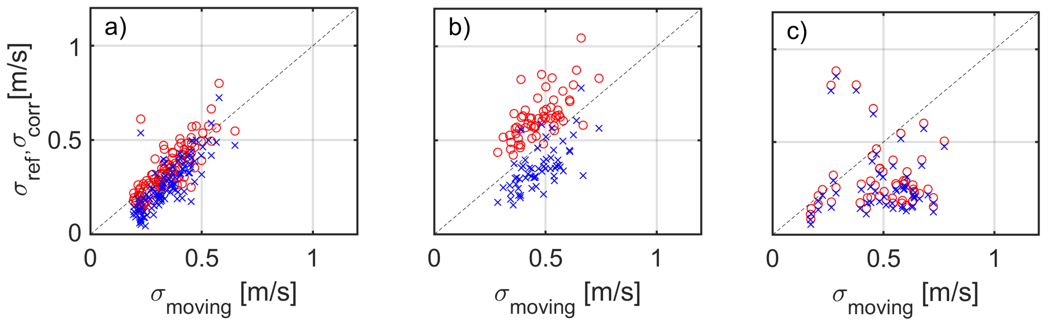
3.3. Analysis of Particular Cases

In order to discuss the goodness of the proposed methodology to estimate the motion-induced HWS standard deviation, this section tackles three representative cases (or bins) from Table 1: cases no. 2, 18, and 25. The first case gave good estimation of the motion-induced HWS standard deviation; the second one, overestimation; and the third one, underestimation.

Figure 4 plots the standard deviation of the HWS with and without correction (Equation (15)), using the lidar on the metmast as reference. The sample size associated with each of these three cases is listed in the “Count no.” column of Table 1.

Figure 4a (case no. 2) shows 247 10-min measurements for which the proposed methodology accurately estimated the standard deviation of the motion-induced HWS error. Before applying Equation (15) correction, uncorrected values fell below the 1:1 line, which indicates that the moving lidar “ saw ” a higher standard deviation. After Equation (15) correction, most of the measurements laid on the 1:1 reference line.

Figure 4b,c, which are representative of case nos. 18 and 25, respectively, show two opposite situations: on one hand, for case no. 18 (Figure 4b), the simulator overestimated the influence of motion and the corrected values laid above the 1:1 line. Further investigation showed that this can be caused by the lack of consistency of the roll/pitch correlation hypothesis (Section 2.4) due to most measurements undergoing bi-modal motion behaviour. On the other hand, case no. 25 (Figure 4c) showed corrected values falling nearly always below the 1:1 line, which means that the estimated correction given by the motion simulator was too low. Further inspection indicated that this underestimation was caused by untrustworthy retrieval of the HWS by the VAD algorithm, as made evident by too-high spatial variation (SV) values from the ZephIR™300 lidar (Figure 5, to be discussed in Section 3.4). The spatial variation is a lidar internal parameter related to the goodness of fit that reveals whether the measurement data is consistent or not with the sinusoidal model assumed by the VAD algorithm. Thus, high SV values are related to a poor VAD fitting, and they are usually found in low HWS, where Taylor’s frozen-eddies hypothesis is no longer true and the lidar does not measure a homogeneous wind along the VAD scanning area.

Table 2. Statistical indicators with and without motion correction for the selected discussion case examples from Table 1. MD stands for mean deviation and RMSE stands for root mean square error (see text and Equations (18) and (19)). MD and RMSE units are (m/s).

Case No.	Count No.	Reference Sonic				Reference Lidar
		Corrected		Uncorrected		Corrected		Uncorrected
		MD	RMSE	MD	RMSE	MD	RMSE	MD	RMSE
2	247	0.08	0.15	0.14	0.19	0.02	0.08	0.08	0.11
18	112	−0.10	0.18	0.14	0.21	−0.12	0.15	0.12	0.15
25	80	0.20	0.26	0.22	0.28	0.20	0.31	0.22	0.33

gives mean difference (MD) and root mean square error (RMSE) indicators for case nos. 2, 18, and 25 in Figure 4 without and with motion correction:

The motion-corrected mean deviation is defined as

$$M{D}_{corr}=\frac{{\displaystyle \sum _i}({\sigma }_{moving,i}-{\sigma }_{corr\left(x\right),i})}{N},$$

(18)

where N is the case “ count no.” (Table 1), ${\sigma }_{moving}$ is the HWS standard deviation measured by the floating lidar (already introduced in Section 3.2), and ${\sigma }_{corr\left(x\right)}$ is the motion-corrected HWS standard deviation (Equation (15)) of the reference instrument, where $x=lidar$ denotes the reference fixed lidar and $x=sonic$ denotes the sonic anemometer. Subscript i is the count-number index, that is, i went from $i=1$ to $i=247$ for case no. 2.

The motion-corrected root mean-square error is defined as

$$RMS{E}_{corr}=\sqrt{\frac{{\displaystyle \sum _i}{({\sigma }_{moving,i}-{\sigma }_{corr\left(x\right),i})}^2}{N}}.$$

(19)

Similarly, uncorrected MD and RMSE indicators are computed by substituting ${\sigma }_{corr\left(x\right),i}$ with ${\sigma }_{ref\left(x\right),i}$, the reference HWS standard deviation, in Equations (18) and (19) above. These indicators are denoted $M{D}_{ref}$ and $RMS{E}_{ref}$, respectively.

The mean deviation gives an estimation of the systematic error, equivalently, the amount of bias, while the RMSE is the quadratic mean of differences, with an ideal value of 0 indicating a perfect fit.

As shown in Table 2, the mean deviation for case no. 2 improved from 0.08 (uncorrected) to 0.02 m/s after motion correction. The RMSE also improved from 0.11 to 0.08 m/s. For overestimation case no. 18, the mean deviation changed sign from 0.12 to −0.12 m/s and, for underestimation case no. 25, the mean deviation virtually did not change (from 0.22 to 0.20 m/s). In over/underestimated case nos. 18 and 25, the RMSE did not improve after motion correction by Equation (15). All things considered, these indicators were consistent with the discussion carried out for Figure 4a–c, and they were therefore used to quantitatively analyse the overall campaign in the following.

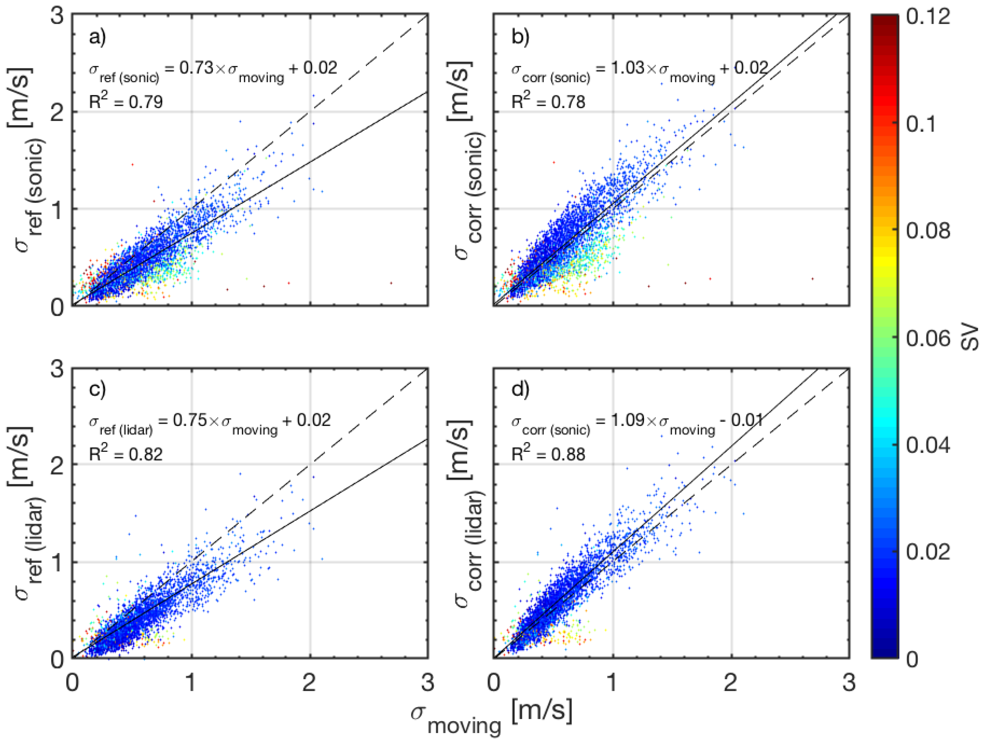
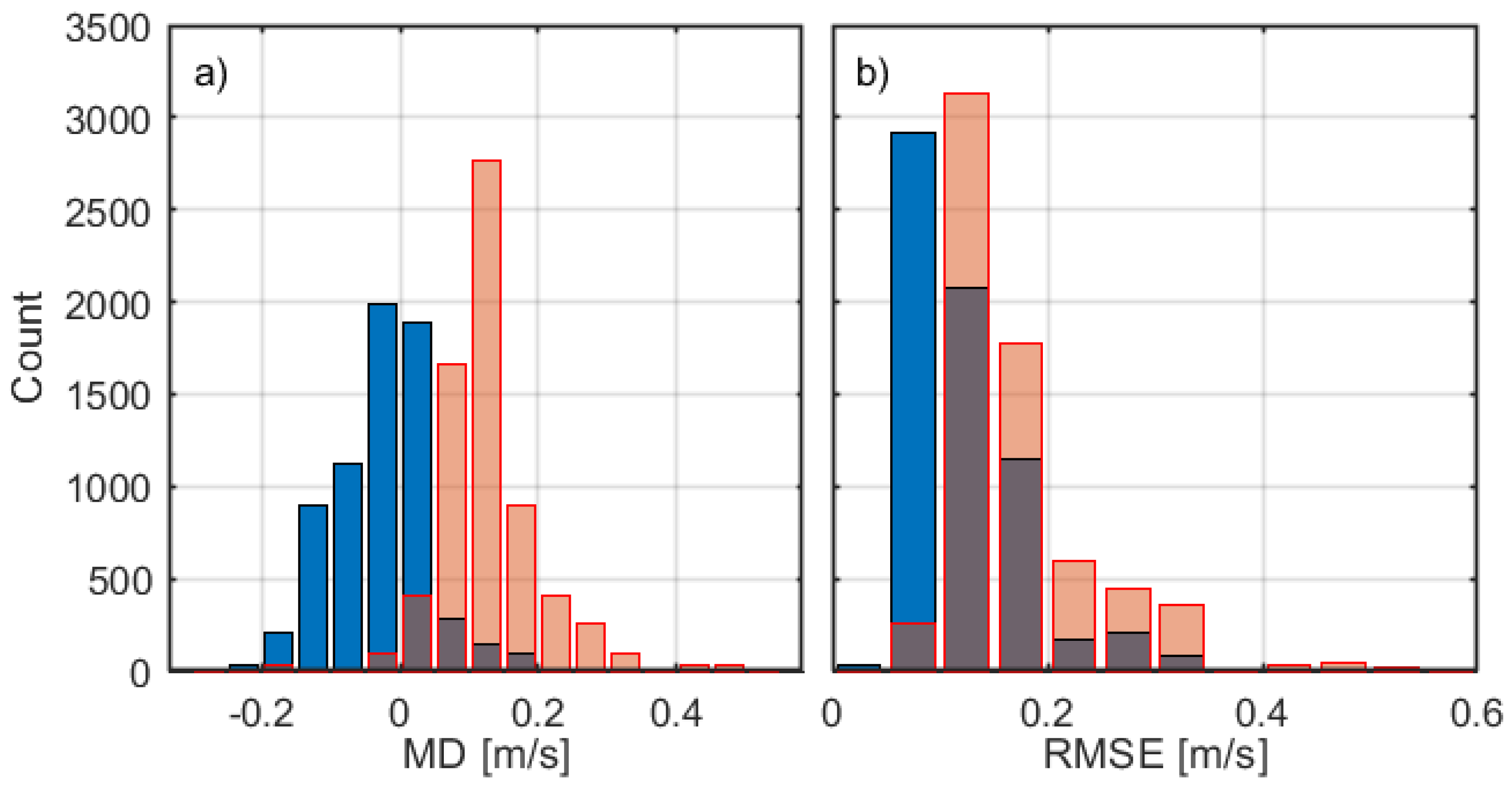
3.4. Analysis of the Whole Campaign

In this section, we discuss overall performance of the motion-corrected HWS standard deviation, ${\sigma }_{corr}$, calculated via Equation (15) and, for comparison, via Equations (16) and (17), for the whole measurement campaign at IJmuiden (6985 10-min records clustered into 109 cases).

In similar fashion to Figure 4 but for the whole campaign, Figure 5 compares the HWS standard deviation of the moving lidar, ${\sigma }_{moving}$, to the motion-corrected standard deviation (Equation (15)) of the sonic and fixed-lidar reference devices (${\sigma }_{corr\left(sonic\right)}$ and ${\sigma }_{corr\left(lidar\right)}$, respectively; right panels) and to the uncorrected ones (left panels; labelled ${\sigma }_{ref\left(sonic\right)}$ and ${\sigma }_{ref\left(lidar\right)}$), respectively). Linear regression parameters and correlation coefficients, superimposed on Figure 5, clearly improved after applying the correction methodology for both the sonic and the fixed-lidar references. Therefore, better agreement between the floating lidar and the instrumental references was obtained. Despite the improvement, there was a tendency to slightly overestimate the motion-corrected standard deviation, ${\sigma }_{corr,\left(x\right)},x=sonic,lidar$, for both the sonic and lidar references.

To further investigate this issue, each point in the scatter plots was colour-coded according to the spatial variation given by the floating lidar. Blue dots, which are associated to low spatial variation, exhibited good correlation while poorly correlated points were associated to spatial-variation figures above 0.06. These high figures were usually due to errors in the VAD-retrieved HWS caused by inhomogeneity of the wind. This means that regression-line results could better approach the ideal 1:1 line by filtering out these outliers on a spatial variation criterion, which is out of the scope of the present work.

To quantitatively discuss the whole campaign via mean difference and root mean square error indicators (Equations (18) and (19),

Table 3. Performance of the variance-combination laws of Section 3.2. (C) stands for linearly correlated variables, (PC) for partially correlated, and (U) for uncorrelated.

	Variance-Combination Law for ${\mathit{\sigma }}_{\mathit{corr}}$						Uncorrected, ${\mathit{\sigma }}_{\mathit{ref}}$
	(C) Equation (17)		(PC) Equation (15)		(U) Equation (16)
	Sonic	Lidar	Sonic	Lidar	Sonic	Lidar	Sonic	Lidar
MD	−0.06	−0.05	−0.03	−0.03	0.08	0.08	0.12	0.13
RMSE	0.17	0.13	0.16	0.12	0.15	0.13	0.18	0.17

presents the results for all 109 cases in the campaign, for both the fixed lidar and sonic references. Results are graphically depicted in the histogram of Figure 6 for the lidar reference only. Figure 6 shows that the motion-uncorrected mean difference, $M{D}_{ref}$, had a positive bias of 0.13 m/s when using the fixed lidar as reference. This bias accounts for the systematic error in the measured HWS standard deviation caused by floating lidar motion as previously reported in [27,59]. After motion correction, the mean difference $M{D}_{corr}$ reduced to the virtually unbiased figure of −0.03 m/s when using the fixed lidar as reference. The negative sign indicates the tendency to overestimate, as mentioned previously. This accounts for an $80\%$ reduction in absolute value. Using the sonic anemometer as reference, the MD reduced from 0.12 to −0.03 m/s (histogram not shown). The RMSE reduced from $RMS{E}_{ref}=0.17$ (uncorrected) to $RMS{E}_{corr}=0.12$ m/s (motion corrected) when using the lidar reference (this accounts for a 29% reduction) and from 0.18 to 0.16 m/s when using the sonic reference. This is considered evidence of the accuracy of the proposed methodology in estimating the motion-induced standard deviation.

As a remark, Figure 7 shows similar HWS motion-corrected results to Figure 5d, but under the limit hypotheses of uncorrelation (Equation (16)) and linear correlation (Equation (17)) between the reference horizontal wind speed, $HWS$, and the motion-induced HWS error, Z. Figure 7 shows that the uncorrelated case and the linear-correlated case can respectively be understood—in a statistical sense over the whole population—as lower (Equation (16)) and upper (Equation (17)) bounds of the proposed motion correction. According to the definition of correlation coefficient, $0<=\left|\rho \right|<=1$, Equation (15) lies in between these two limit cases ($\rho =0$, $\rho =1$). This is corroborated in Table 3, which shows MD and RMSE indicators when the lidar and the sonic anemometer are used as references, for the three combination hypotheses discussed in Section 3.2: partially correlated (PC), uncorrelated (U) and correlated (C) variables. It emerges that the approximation of partial correlation yielded the best results, as shown by the lowest MD and RMSE figures in Table 3.

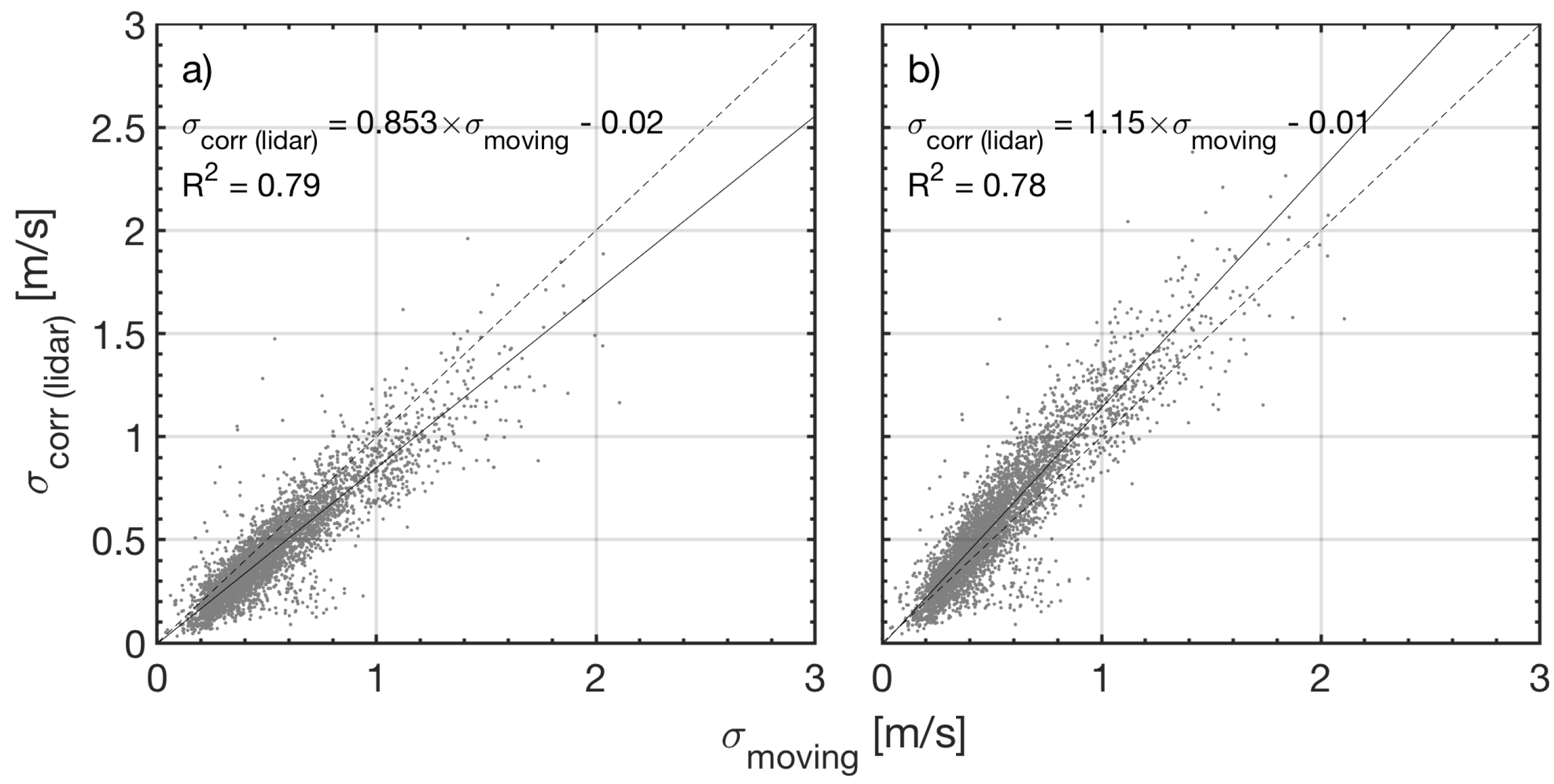
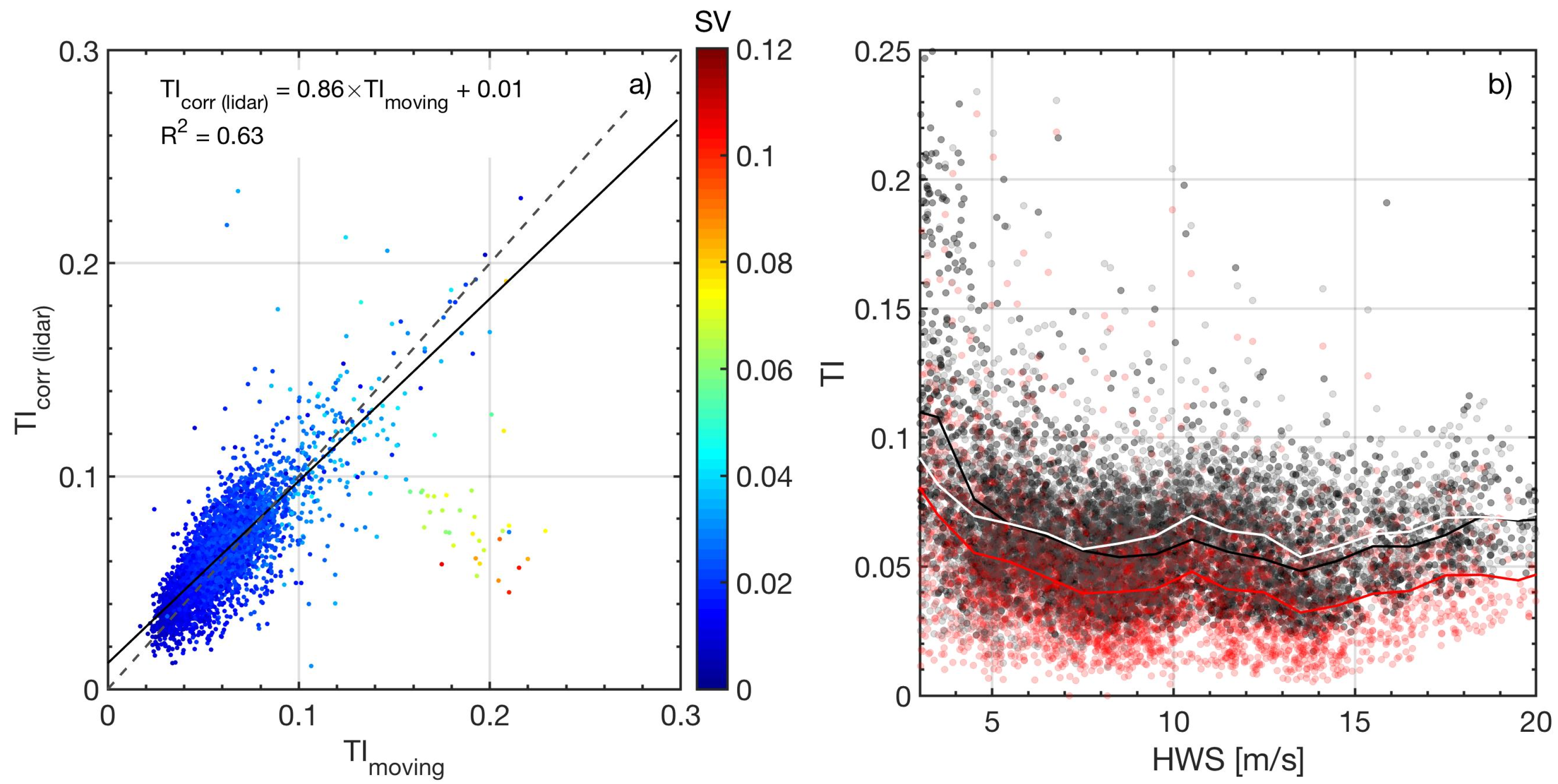
3.5. Turbulence Intensity

Analogously to Figure 5d, Figure 8a compares the TI of the floating lidar, $T{I}_{moving}$, to the motion-corrected TI of the fixed-lidar reference, $T{I}_{corr\left(lidar\right)}$. Dots are colour-coded according to their spatial variation parameter. HWSs below 3 m/s, which are usually out of the production regime of commercial wind turbines and tend to numerically distort the TI, were filtered out to enhance the readability of the graph. Although some scattering is present in the pattern of dots, the regression line (slope = 0.86, intercept = 0.01) shows a similar tendency to that of Figure 5d of approaching the 1:1 line after motion correction. Quantitatively, by defining similar MD and RMSE indicators for the TI (counterpart of Equations (18) and (19) by changing standard deviation, $\sigma$, into TI), the MD for the moving lidar reduced from 0.016 (uncorrected) to 0.003 (motion corrected). In terms of RMSE, the reduction was from 0.018 to 0.012, which despite being not very important implies an approximate 30% reduction in the dispersion of data. In addition, most of the points falling far from the 1:1 line had high spatial variation figures, typically SV > 0.06, which is characteristic of low HWS.

Figure 8b illustrates the successful application of the motion-correction algorithm by superimposing: (i) the TI measured by the uncorrected fixed-lidar reference ($T{I}_{ref\left(lidar\right)}$, red); (ii) the TI derived from the motion-corrected lidar reference ($T{I}_{corr\left(lidar\right)}$, grey); and (iii) the TI measured by the moving floating lidar ($T{I}_{moving}$, black) as a function of the 10-min HWS. To aid visual interpretation, average TIs using a 1.0 m/s binwidth were also plotted in red, white, and black traces, respectively. As expected, the apparent TI measured by the floating lidar (black trace) was higher than the true one measured by the reference lidar (red trace). After application of motion correction to the reference TI, $T{I}_{ref\left(lidar\right)}$ (red dots/red trace), the motion-corrected TI, $T{I}_{corr\left(lidar\right)}$ (grey dots/white trace), approximately followed the floating lidar TI, $T{I}_{moving}$ (black dots/black trace). At this point, it must be said that, in practice, the correction is to be applied to the TI measured by the floating lidar so as to shift it down. However, this does not change the line of reasoning. Quantitatively, the mean value of the TI measured by the fixed lidar in the 3–20 m/s HWS range was $T{I}_{ref\left(lidar\right)}=0.047$ and the TI measured by the floating lidar was $T{I}_{moving}=0.065$. After motion correction, the mean value of the reference-corrected TI was $T{I}_{corr\left(lidar\right)}=0.067$, which was only −0.002 apart from $T{I}_{moving}$ and drastically reduced the initial difference between floating lidar and the reference lidar TI from 0.018 to −0.002. These differences account for an error reduction from 38.3% to 4.3%.

As discussed in Section 1, in order to improve the design layout of offshore wind farms and selection of the appropriate wind turbine model, turbulence intensity measurements of a floating lidar are needed. Performance results from Section 3.4 and Section 3.5 showed that, in the environmental conditions considered, the proposed methodology has the potential to estimate the influence of motion on TI measurements with the ZephIR™300 lidar.

4. Conclusions

We presented a methodology to estimate the 10-min motion-induced standard deviation and turbulence intensity on the retrieved HWS for a ZephIR™300 lidar at a given measurement height without accessing individual line-of-sight information of the lidar scanning pattern or individual 1-s data.

The proposed methodology includes a software-based motion simulator that reproduces the VAD algorithm used to retrieve the HWS under simple-harmonic motional conditions and a moment-computation recursive procedure to estimate the motion-induced HWS error standard deviation, ${\sigma }_Z$, as well as the motion-induced TI.

The motion simulator input parameters are the 10-min average HWS and 10-min motional amplitude and period of the floating lidar buoy as well as initial roll/pitch motional phases and lidar scan phase (${\varphi }_r$, ${\varphi }_p$, and ${\varphi }_s$, respectively). A binning procedure is used to group measurement records into bins with similar HWS and motional conditions. The procedure is aimed at computing the 10-min HWS error standard deviation in each bin by internally sweeping these phases in the $[0,2\pi )$ range, which therefore become blind inputs to the user.

The method relies on the approximation that roll/pitch amplitudes and periods are linearly correlated on a 10-min basis and that, consequently, only one motional amplitude and period is needed. This one-degree-of-freedom approximation combined with that of simple harmonic motion are the main limitations of the method. Under these hypotheses, the motion-induced HWS standard deviation was proven to be independent of wind direction, which allows this variable to be neglected in the computations (wind direction errors caused by yaw motion are always corrected by means of the buoy compass).

According to error-propagation laws, the motion-corrected HWS standard deviation (Equation (15)), which combines the motion-induced HWS error and the reference HWS, was shown to depend on the correlation between these two variables and the degree of approximation by which it is estimated. Uncorrelated ($\rho =0$) and linearly-correlated ($\left|\rho \right|=1$) sub-cases were interpreted as upper and lower bounds of the motion-corrected HWS standard deviation, respectively.

The performance of the proposed methodology was tested as part of a 60-day study period at offshore metmast IJmuiden by using a sonic anemometer and a fixed lidar as reference instruments. The motion-corrected HWS standard deviation and that of the reference HWS (from either the fixed lidar or the sonic anemometer) were compared to the measured floating-lidar HWS standard deviation for the 109 most frequent cases of the campaign. This indicated an overall improvement in the average MD from 0.13 (uncorrected) to −0.03 m/s (motion corrected) and an average RMSE reduction from 0.17 to 0.12 m/s, which essentially means that the floating-lidar and the motion-corrected HWS standard deviation laid on the ideal 1:1 line with a dispersion equal to the RMSE.

When analysing the whole campaign as a function of the spatial variation, the most poorly correlated points were associated with mid-to-high spatial variations (SV > 0.06). Wider dispersion arose when using the sonic anemometer as reference, which was caused by the inherently different wind measurement principle of the sonic as compared to the lidar. Analysis in terms of TI showed similar improvement, made evident by a reduction in the difference between the reference-lidar and the floating-lidar TI from 0.018 (uncorrected) to −0.002 (motion corrected).

Despite these good results, they must be interpreted with caution because performance is based on MD and RMSE criteria over the whole statistical sample and not on an individual measurement basis. Overall, in the environmental conditions considered, the proposed methodology holds promise for use in the estimation of the influence of motion on TI measurements with the ZephIR™300 lidar. These results should be extended to other conditions and set-ups, which, if proven effective, could eventually be used to correct TI measurements of floating lidars as standalone devices.

References

1. Global Wind Energy Council. Global Wind Energy Outlook 2016; Technical Report; Global Wind Energy Council: Brussels, Belgium, 2016. [Google Scholar]
2. Global Wind Energy Council. Global Wind Energy Rerport 2016: Annual Market Update; Technical Report; Global Wind Energy Council: Brussels, Belgium, 2017. [Google Scholar]
3. Roland Berger. Offshore Wind toward 2020: On the Pathway to Cost Competitiveness; Technical Report; Roland Berger: Munich, Germany, 2013. [Google Scholar]
4. Barthelmie, R.; Pryor, S. Can Satellite Sampling of Offshore Wind Speeds Realistically Represent Wind Speed Distributions? J. Appl. Meteorol. 2003, 42, 83–94. [Google Scholar] [CrossRef]
5. Chang, R.; Zhu, R.; Badger, M.; Hasager, C.B.; Zhou, R.; Ye, D.; Zhang, X. Applicability of Synthetic Aperture Radar wind retrievals on offshore wind resources assessment in Hangzhou Bay, China. Energies 2014, 7, 3339–3354. [Google Scholar] [CrossRef]
6. Hirth, B.D.; Schroeder, J.L.; Gunter, W.S.; Guynes, J.G. Measuring a utility-scale turbine wake using the TTUKa mobile research radars. J. Atmos. Ocean. Technol. 2012, 29, 765–771. [Google Scholar] [CrossRef]
7. Barthelmie, R.; Folkerts, L.; Ormel, F.; Sanderhoff, P.; Eecen, P.; Stobbe, O.; Nielsen, N. Offshore wind turbine wakes measured by SODAR. J. Atmos. Ocean. Technol. 2003, 20, 466–477. [Google Scholar] [CrossRef]
8. Vogt, S.; Thomas, P. SODAR—A useful remote sounder to measure wind and turbulence. J. Wind Eng. Ind. Aerodyn. 1995, 54, 163–172. [Google Scholar] [CrossRef]
9. Lang, S.; McKeogh, E. LIDAR and SODAR Measurements of Wind Speed and Direction in Upland Terrain for Wind Energy Purposes. Remote Sens. 2011, 3, 1871–1901. [Google Scholar] [CrossRef] [Green Version]
10. International Energy Association. State of the Art of Remote Wind Speed Sensing Techniques Using Sodar, Lidar and Satellites; Technical Report; International Energy Association: Paris, France, 2007. [Google Scholar]
11. Sempreviva, A.M.; Barthelmie, R.J.; Pryor, S.C. Review of Methodologies for Offshore Wind Resource Assessment in European Seas. Surv. Geophys. 2008, 29, 471–497. [Google Scholar] [CrossRef]
12. Scholbrock, A.; Fleming, P.; Schlipf, D.; Wright, A.; Johnson, K.; Wang, N. Lidar-Enhanced Wind Turbine Control: Past, Present, and Future. In Proceedings of the 2016 American Control Conference (ACC), Boston, MA, USA, 6–8 July 2016; pp. 1399–1406. [Google Scholar]
13. Rodrigo, J.S. State-of-the-Art of Wind Resource Assessment. Deliverable D7, CENER. 2010. Available online: https://cordis.europa.eu/project/rcn/93290_en.html (accessed on 14 December 2012).
14. Clifton, A.; Courtney, M. 15. Ground-Based Vertically Profiling Remote Sensing for Wind Reource Assessment; Technical Report; IEA Wind Expert Group Study on Recommended Practices; IEA: Paris, France, 2013. [Google Scholar]
15. Li, J.; Yu, X.B. LiDAR technology for wind energy potential assessment: Demonstration and validation at a site around Lake Erie. Energy Convers. Manag. 2017, 144, 252–261. [Google Scholar] [CrossRef]
16. Trabucchi, D.; Trujillo, J.J.; Kühn, M. Nacelle-based Lidar Measurements for the Calibration of a Wake Model at Different Offshore Operating Conditions. Energy Procedia 2017, 137, 77–88. [Google Scholar] [CrossRef]
17. Krishnamurthy, R.; Reuder, J.; Svardal, B.; Fernando, H.; Jakobsen, J. Offshore Wind Turbine Wake characteristics using Scanning Doppler Lidar. Energy Procedia 2017, 137, 428–442. [Google Scholar] [CrossRef]
18. van Dooren, M.; Trabucchi, D.; Kühn, M. A Methodology for the Reconstruction of 2D Horizontal Wind Fields of Wind Turbine Wakes Based on Dual-Doppler Lidar Measurements. Remote Sens. 2016, 8, 809. [Google Scholar] [CrossRef]
19. International Electrotechnical Commission. IEC 61400-12 Wind Turbine Power Performance Testing; Technical Report; International Electrotechnical Commission: Geneva, Switzerland, 1998. [Google Scholar]
20. Williams, B.M. New Applications of Remote Sensing Technology for Offshore Wind Powert. Master’s Thesis, University Delawre, Newark, DE, USA, 2013. [Google Scholar]
21. Pichugina, Y.L.; Banta, R.M.; Brewer, W.A.; Sandberg, S.P.; Hardesty, R.M. Doppler Lidar–Based Wind-Profile Measurement System for Offshore Wind-Energy and Other Marine Boundary Layer Applications. J. Appl. Meteorol. Climatol. 2011, 51, 327–349. [Google Scholar] [CrossRef]
22. Courtney, M.S.; Hasager, C.B. Remote sensing technologies for measuring offshore wind. In Offshore Wind Farms; Elsevier: Amsterdam, The Netherlands, 2016; Chapter 4; pp. 59–82. [Google Scholar]
23. Antoniou, I.; Jorgensen, H.E.; Mikkelsen, T.; Frandsen, S.; Barthelmie, R.; Perstrup, C.; Hurtig, M. Offshore wind profile measurements from remote sensing instruments. In Proceedings of the European Wind Energy Association Conference & Exhibition, Athens, Greece, 27 February–2 March 2006. [Google Scholar]
24. Carbon Trust. Carbon Trust Offshore Wind Accelerator Roadmap for the Commercial Acceptance of Floating LIDAR Technology; Technical Report; Carbon Trust: London, UK, 2013. [Google Scholar]
25. Clifton, A.; Clive, P.; Gottschall, J.; Schlipf, D.; Simley, E.; Simmons, L.; Stein, D.; Trabucchi, D.; Vasiljevic, N.; Würth, I. IEA Wind Task 32: Wind Lidar Identifying and Mitigating Barriers to the Adoption of Wind Lidar. Remote Sens. 2018, 10, 406. [Google Scholar] [CrossRef]
26. Bischoff, O.; Wurth, I.; Gottschall, J.; Gribben, B.; Hughes, J.; Stein, D.; Verhoef, H. Recommended Practices for Floating Lidar Systems; Technical Report; IEA Wind Task 32; IEA: Paris, France, 2016. [Google Scholar]
27. Gottschall, J.; Wolken-Möhlmann, G.; Viergutz, T.; Lange, B. Results and conclusions of a floating-lidar offshore test. Energy Procedia 2014, 53, 156–161. [Google Scholar] [CrossRef]
28. Schuon, F.; González, D.; Rocadenbosch, F.; Bischoff, O.; Jané, R. KIC InnoEnergy Project Neptune: Development of a Floating LiDAR Buoy for Wind, Wave and Current Measurements. In Proceedings of the DEWEK 2012 German Wind Energy Conference, Bremen, Germany, 7–8 November 2012. [Google Scholar]
29. Sospedra, J.; Cateura, J.; Puigdefàbregas, J. Novel multipurpose buoy for offshore wind profile measurements EOLOS platform faces validation at ijmuiden offshore metmast. Sea Technol. 2015, 56, 25–28. [Google Scholar]
30. Mathisen, J.P. Measurement of wind profile with a buoy mounted lidar. Energy Procedia 2013, 30, 12. [Google Scholar]
31. Kyriazis, T. Low cost and flexible offshore wind measurements using a floating lidar solution (FLIDAR™). In Proceedings of the EWEA Conference, Vienna, Austria, 4–7 February 2013. [Google Scholar]
32. Hung, J.B.; Hsu, W.Y.; Chang, P.C.; Yang, R.Y.; Lin, T.H. The performance validation and operation of nearshore wind measurements using the floating lidar. Coast. Eng. Proc. 2014, 1, 11. [Google Scholar] [CrossRef]
33. Hsuan, C.Y.; Tasi, Y.S.; Ke, J.H.; Prahmana, R.A.; Chen, K.J.; Lin, T.H. Validation and Measurements of Floating LiDAR for Nearshore Wind Resource Assessment Application. Energy Procedia 2014, 61, 1699–1702. [Google Scholar] [CrossRef]
34. Gottschall, J.; Gribben, B.; Stein, D.; Würth, I. Floating lidar as an advanced offshore wind speed measurement technique: Current technology status and gap analysis in regard to full maturity. Wiley Interdiscip. Rev. Energy Environ. 2017, 6. [Google Scholar] [CrossRef]
35. Gottschall, J.; Wolken-Möhlmann, G.; Lange, B. About offshore resource assessment with floating lidars with special respect to turbulence and extreme events. J. Phys. Conf. Ser. 2014, 555, 012043. [Google Scholar] [CrossRef] [Green Version]
36. Mangat, M.; des Roziers, E.B.; Medley, J.; Pitter, M.; Barker, W.; Harris, M. The impact of tilt and inflow angle on ground based lidar wind measurements. In Proceedings of the EWEA 2014, Barcelona, Spain, 10–13 March 2014. [Google Scholar]
37. Pitter, M.; Burin des Roziers, E.; Medley, J.; Mangat, M.; Slinger, C.; Harris, M. Performance Stability of Zephir in High Motion Enviroments: Floating and Turbine Mounted. Available online: https://bit.ly/2EuDY5i (accessed on 14 December 2018).
38. Wolken-Möhlmann, G.; Lilov, H.; Lange, B. Simulation of motion induced measurement errors for wind measurements using LIDAR on floating platforms. Fraunhofer IWES Am Seedeich 2011, 45, 27572. [Google Scholar]
39. Bischoff, O.; Würth, I.; Cheng, P.; Tiana-Alsina, J.; Gutiérrez, M. Motion effects on lidar wind measurement data of the EOLOS buoy. In Proceedings of the First International Conference on Renewable Energies Offshore, Lisbon, Portugal, 24–26 November 2014. [Google Scholar]
40. Tiana-Alsina, J.; Rocadenbosch, F.; Gutierrez-Antunano, M.A. Vertical Azimuth Display simulator for wind-Doppler lidar error assessment. In Proceedings of the 2017 IEEE International Geoscience and Remote Sensing Symposium (IGARSS), Fort Worth, TX, USA, 23–28 July 2017. [Google Scholar] [CrossRef]
41. Nicholls-Lee, R. A low motion floating platform for offshore wind resource assessment using Lidars. In Proceedings of the ASME 2013 32nd International Conference on Ocean, Offshore and Arctic Engineering, Nantes, France, 9–14 June 2013. [Google Scholar]
42. Tiana-Alsina, J.; Gutiérrez, M.A.; Würth, I.; Puigdefàbregas, J.; Rocadenbosch, F. Motion compensation study for a floating Doppler wind lidar. In Proceedings of the Geoscience and Remote Sensing Symposium, Milan, Italy, 26–31 July 2015. [Google Scholar]
43. Bischoff, O.; Schlipf, D.; Würth, I.; Cheng, P. Dynamic Motion Effects and Compensation Methods of a Floating Lidar Buoy. In Proceedings of the EERA DeepWind 2015 Deep Sea Offshore Wind Conference, Trondheim, Norway, 4–6 February 2015. [Google Scholar]
44. Gottschall, J.; Lilov, H.; Wolken-Möhlmann, G.; Lange, B. Lidars on floating offshore platforms; about the correction of motion-induced lidar measurement errors. In Proceedings of the EWEA 2012, Copenhagen, Denmark, 16–19 April 2012. [Google Scholar]
45. International Electrotechnical Commission. IEC 61400-1 2005 Wind Turbine Power Performance Testing; Technical Report; International Electrotechnical Commission: Geneva, Switzerland, 2005. [Google Scholar]
46. Manwell, J.F.; McGowan, J.G.; Rogers, A.L. Wind Energy Explained: Theory, Design and Application; Number Book, Whole; Wiley: Chichester, UK, 2009. [Google Scholar]
47. Hansen, K.S.; Barthelmie, R.J.; Jensen, L.E.; Sommer, A. The impact of turbulence intensity and atmospheric stability on power deficits due to wind turbine wakes at Horns Rev wind farm. Wind Energy 2012, 15, 183–196. [Google Scholar] [CrossRef]
48. Sathe, A.; Mann, J.; Gottschall, J.; Courtney, M. Can wind lidars measure turbulence? J. Atmos. Ocean. Technol. 2011, 28, 853–868. [Google Scholar] [CrossRef]
49. Sathe, A. Influence of Wind Conditions on Wind Turbine Loads and Measurements of Turbulence Using Lidars. Ph.D. Thesis, Delft University, Delft, The Netherlands, 2012. [Google Scholar]
50. Sathe, A.; Banta, R.; Pauscher, L.; Vogstad, K.; Schilpf, D.; Wylie, S. Estimating Turbulence Statistics and Parameters from Ground- and Nacelle-Based Lidar Measurements; Technical Report; Technical University of Denmark: Lyngby, Denmark, 2015. [Google Scholar]
51. Wagner, R.; Mikkelsen, T.; Courtney, M. Investigation of Turbulence Measurements With a Continuous Wave, Conically Scanning LiDAR; Technical Report; DTU: Lyngby, Denmark, 2009. [Google Scholar]
52. Henderson, S.W.; Gatt, P.; Rees, D.; Huffaker, M. Wind LIDAR. In Laser Remote Sensing; Optical Science and Engineering; CRC Press: Boca Raton, FL, USA, 2005; Chapter 7. [Google Scholar]
53. Gutierrez-Antunano, M.A.; Tiana-Alsina, J.; Rocadenbosch, F.; Sospedra, J.; Aghabi, R.; Gonzalez-Marco, D. A wind-lidar buoy for offshore wind measurements: First commissioning test-phase results. In Proceedings of the 2017 IEEE International Geoscience and Remote Sensing Symposium (IGARSS), Fort Worth, TX, USA, 23–28 July 2017. [Google Scholar] [CrossRef]
54. Werkhoven, E.J.; Verhoef, J.P. Offshore Meteorological Mast Ijmuiden Abstract of Instrumentation Report. Available online: https://bit.ly/2PCjjxg (accessed on 14 December 2018).
55. Poveda, J.; Wouters, D.; Nederland, S.E.C. Wind Measurements at Meteorological Mast Ijmuiden. Available online: https://bit.ly/2QYbqHj (accessed on 14 December 2018).
56. Clifford, S.F.; Kaimal, J.C.; Lataitis, R.J.; Strauch, R.G. Ground-based remote profiling in atmospheric studies: An overview. Proc. IEEE 1994, 82, 313–355. [Google Scholar] [CrossRef]
57. Barlow, R.J. Statistics: A Guide to the Use of Statistical Methods in the Physical Sciences; Manchester Physics Series; Wiley: Chichester, UK, 1989. [Google Scholar]
58. Papoulis, A. Probability, Random Variables, and Stochastic Processes; McGraw-Hill: New York, NY, USA, 1965. [Google Scholar]
59. Gutiérrez-Antuñano, M.A.; Tiana-Alsina, J.; Rocadenbosch, F. Performance evaluation of a floating lidar buoy in nearshore conditions. Wind Energy 2017, 20, 1711–1726. [Google Scholar] [CrossRef] [Green Version]
Figure 1. Simulated horizontal wind speed (HWS) error, Z (Equation (1)), under roll-only motion as a function of velocity-azimuth-display (VAD) scan phase (x-axis) and motional period, T, (y-axis). Roll phase ( ϕ r ) is equal to 0 deg (a), 90 deg (b), 180 deg (c), and 270 deg (d). Roll amplitude is 3.5 deg, wind vector is ( 0 , 10 , 0 ) m/s, and measurement height is 100 m in all panels [40].
Remotesensing 10 02037 g001
Figure 2. Scatter plots for 10-min-averaged roll and pitch angles. (a) angular amplitude; (b) angular period. Dashed lines correspond to the 1:1 reference line. Insets show the roll–pitch cross-covariance for different time lags.
Remotesensing 10 02037 g002
Figure 3. Simulator results of motion-induced HWS error standard deviation, σ Z as a function of motional period, T (x-axis) and wind direction (y-axis). HWS is 10 m/s HWS, roll-and-pitch amplitude is 3.5 deg.
Remotesensing 10 02037 g003
Figure 4. Selected discussion case examples from Table 1. (a) case no. 2, HWS = 5 m/s; angular amplitude (AA) = 2 deg; period (T) = 4 s; (b) case no. 18, HWS = 9 m/s; AA = 3 deg; T = 3 s; (c) case no. 25, HWS = 3 m/s; AA = 1 deg; T = 3 s). All panels: the x-axis represents the 10-min HWS standard deviation of the floating lidar, denoted σ m o v i n g . The y-axis represents (in blue crosses) the standard deviation of the reference-lidar HWS (denoted σ r e f ) and (in red circles) the standard deviation of the motion-corrected HWS (denoted σ c o r r ). The dashed black line represents the 1:1 reference line.
Remotesensing 10 02037 g004
Figure 5. Analysis of the whole campaign (109 cases, 6985 10-min measurement records) by using as reference the sonic anemometer (a) and the lidar on metmast (b), without motion correction (c); σ r e f ( s o n i c / l i d a r ) in the y-axis) and with motion correction (d); σ c o r r ( s o n i c / l i d a r in the y-axis). The x-axis represents the HWS standard deviation of the floating lidar, denoted σ m o v i n g . Each point is a 10-min record. Dashed lines represent the 1:1 line. Solid lines plot the regression lines. Colour bar indicates spatial variation.
Remotesensing 10 02037 g005
Figure 6. Histogram of the main statistical parameters. (a) mean difference; (b) root mean square error using the fixed lidar as reference; for all panels: blue = motion corrected, red = uncorrected.
Remotesensing 10 02037 g006
Figure 7. Comparison between 10-min floating-lidar HWS standard deviation measurements and motion-corrected ones by using Equation (16) versus Equation (17). (a) uncorrelation hypothesis (Equation (16)); (b) linear-correlation hypothesis (Equation (17)). The dashed line indicates the 1:1 line and the solid line shows the linear regression.
Remotesensing 10 02037 g007
Figure 8. Turbulence intensity (TI) results for the whole campaign. (a) comparison between the motion-corrected TI of the fixed-lidar reference, T I c o r r ( l i d a r ) and the floating-lidar TI, T I m o v i n g . The colour bar indicates spatial variation. The dashed line indicates the 1:1 line; (b) plots of TI versus HWS (see text): Red dots = uncorrected fixed-lidar reference, T I r e f ( l i d a r ) . Grey dots = motion-corrected lidar reference, T I c o r r ( l i d a r ) . Black dots = floating lidar, T I m o v i n g . Traces with the same colours plot average TIs using a 1.0-m/s binwidth.
Remotesensing 10 02037 g008