Satellite-Based Mapping of Cultivated Area in Gash Delta Spate Irrigation System, Sudan

Abstract
:
1. Introduction
2. Study Area and Data
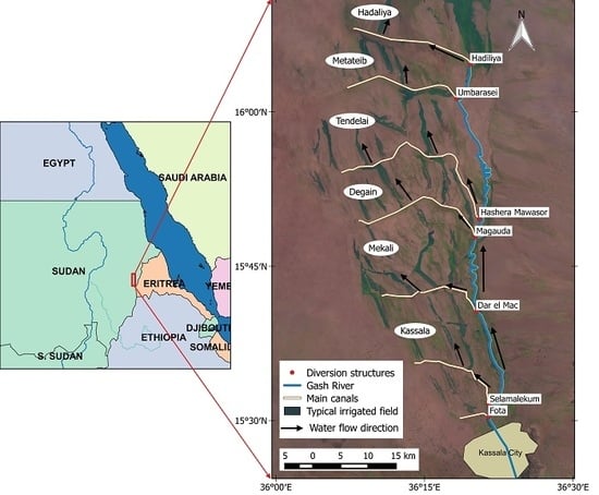
2.1. Study Area
2.2. Data
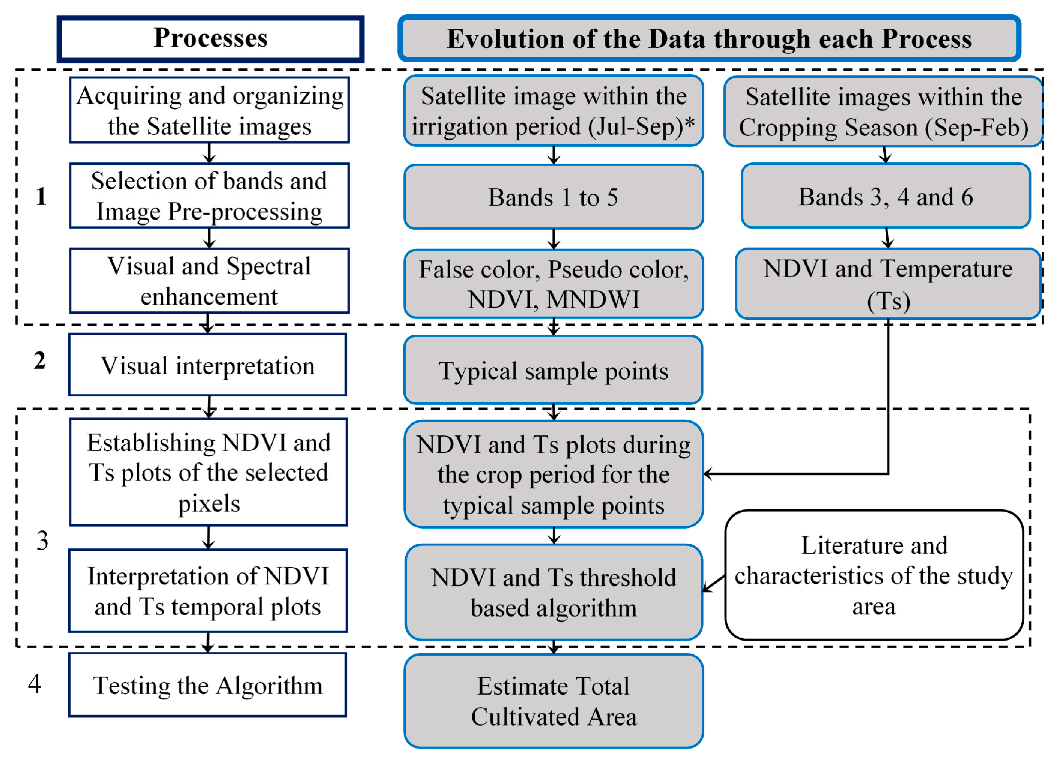
3. Methods
3.1. Image Preparation and Enhancement
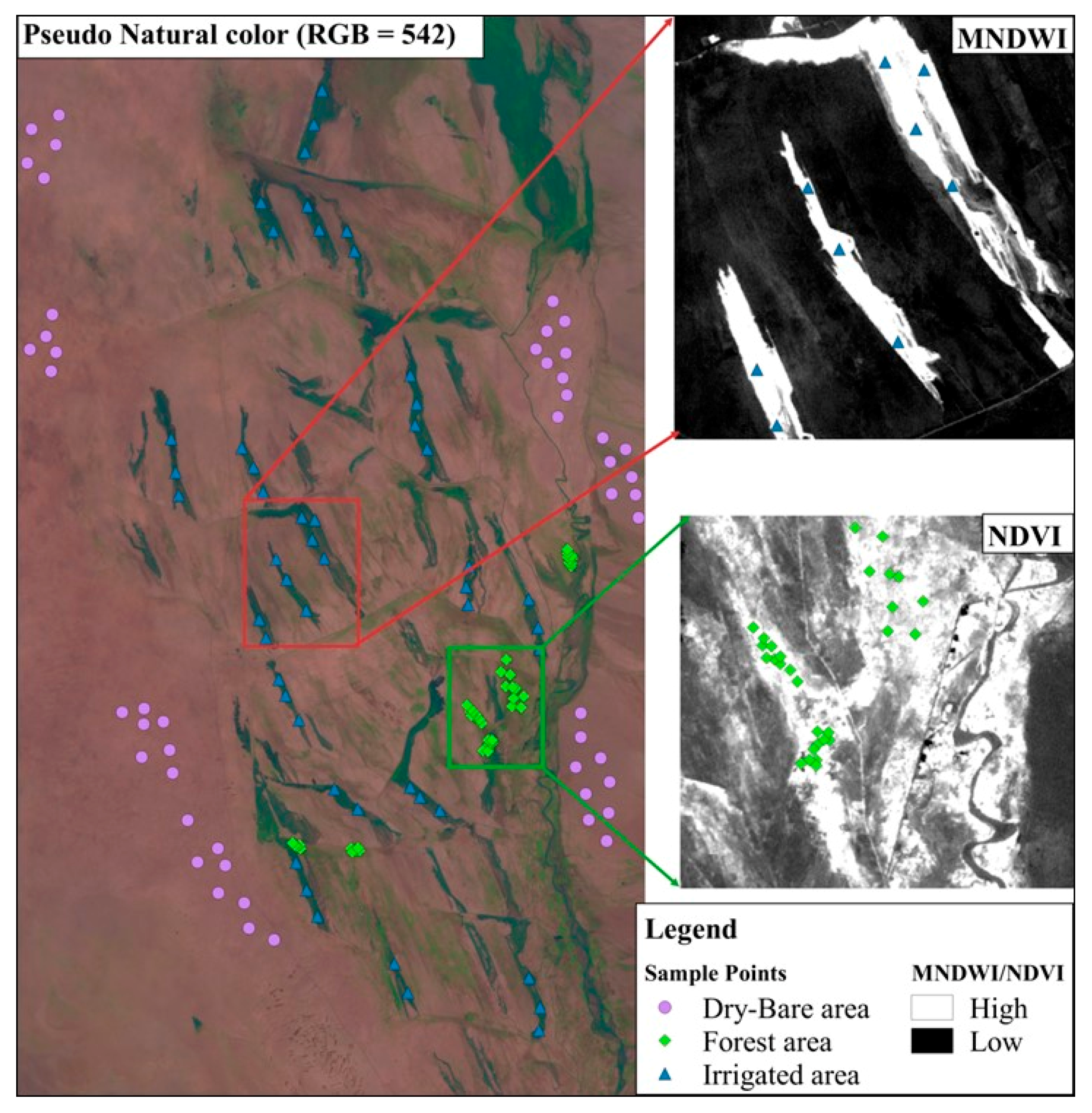
3.2. Identification and Selection of Sample Points
3.3. Building the Classification Algorithm
3.4. Verification of Results
4. Results and Discussion
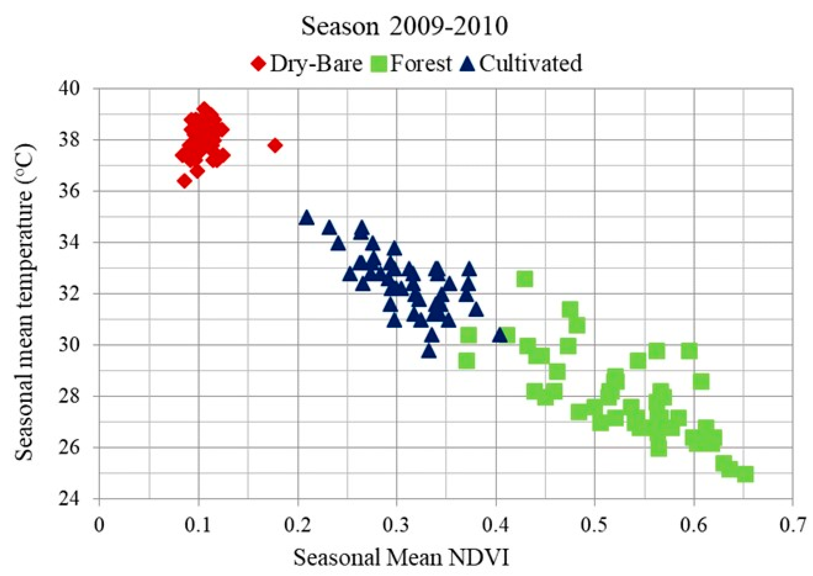
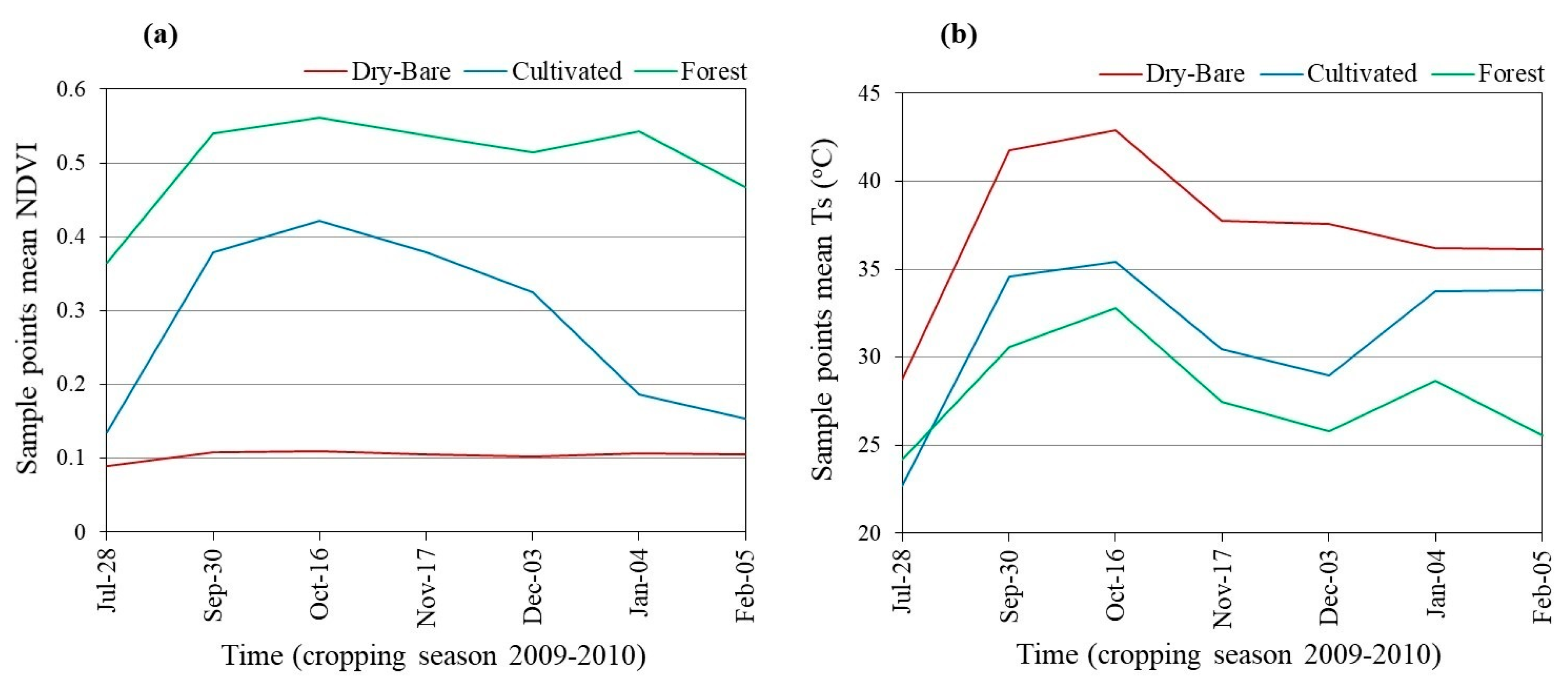
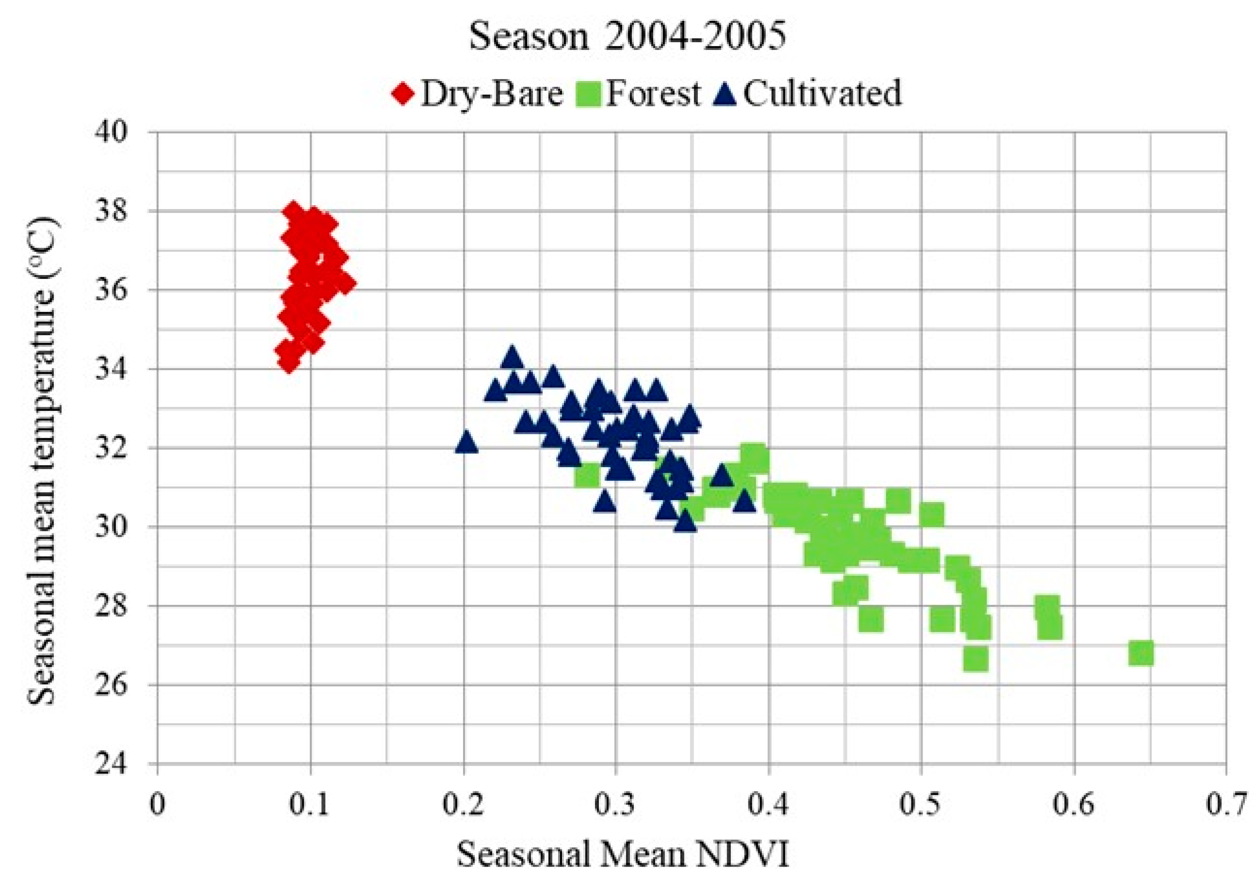
4.1. Identification and Selection of Sample Points
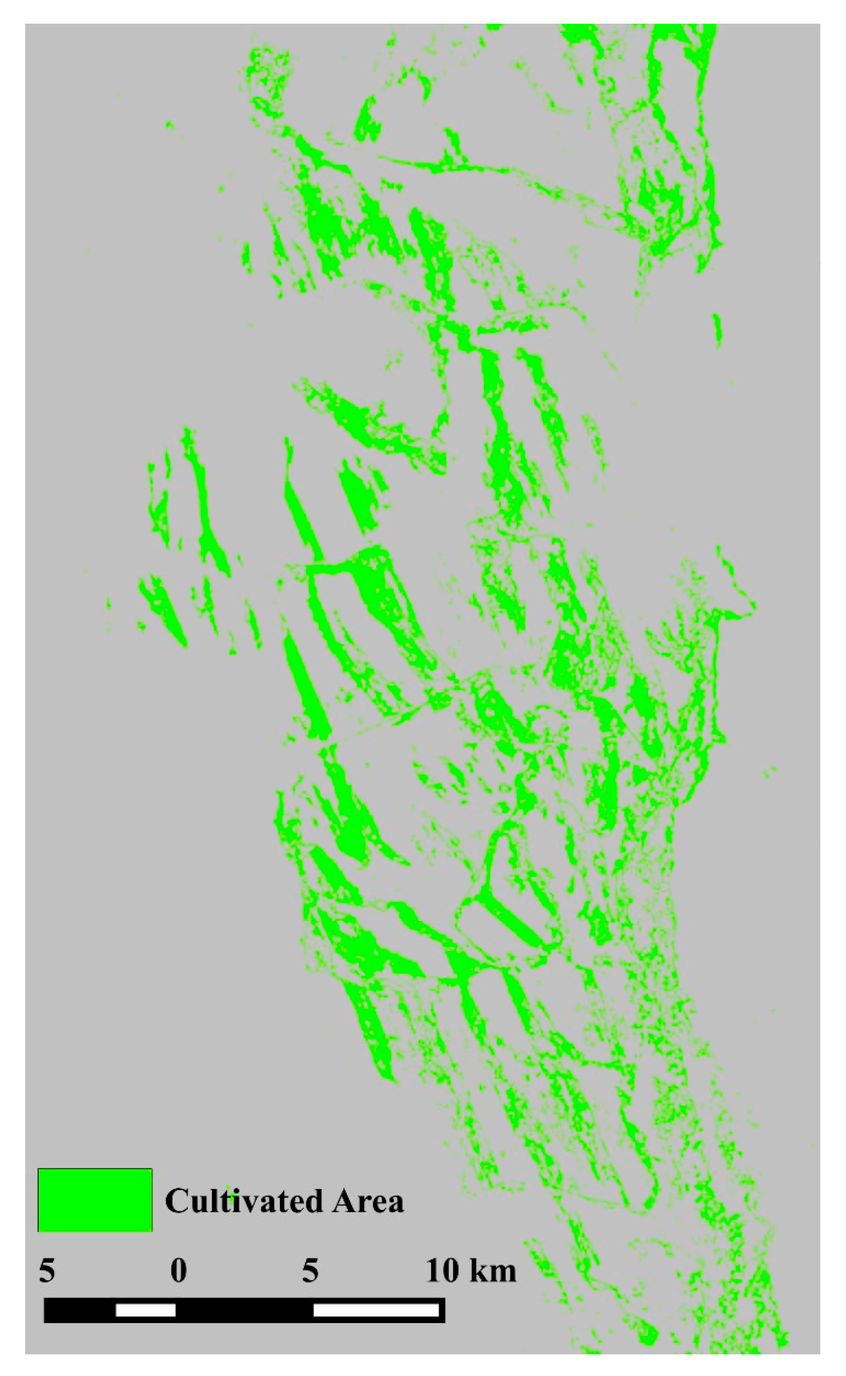
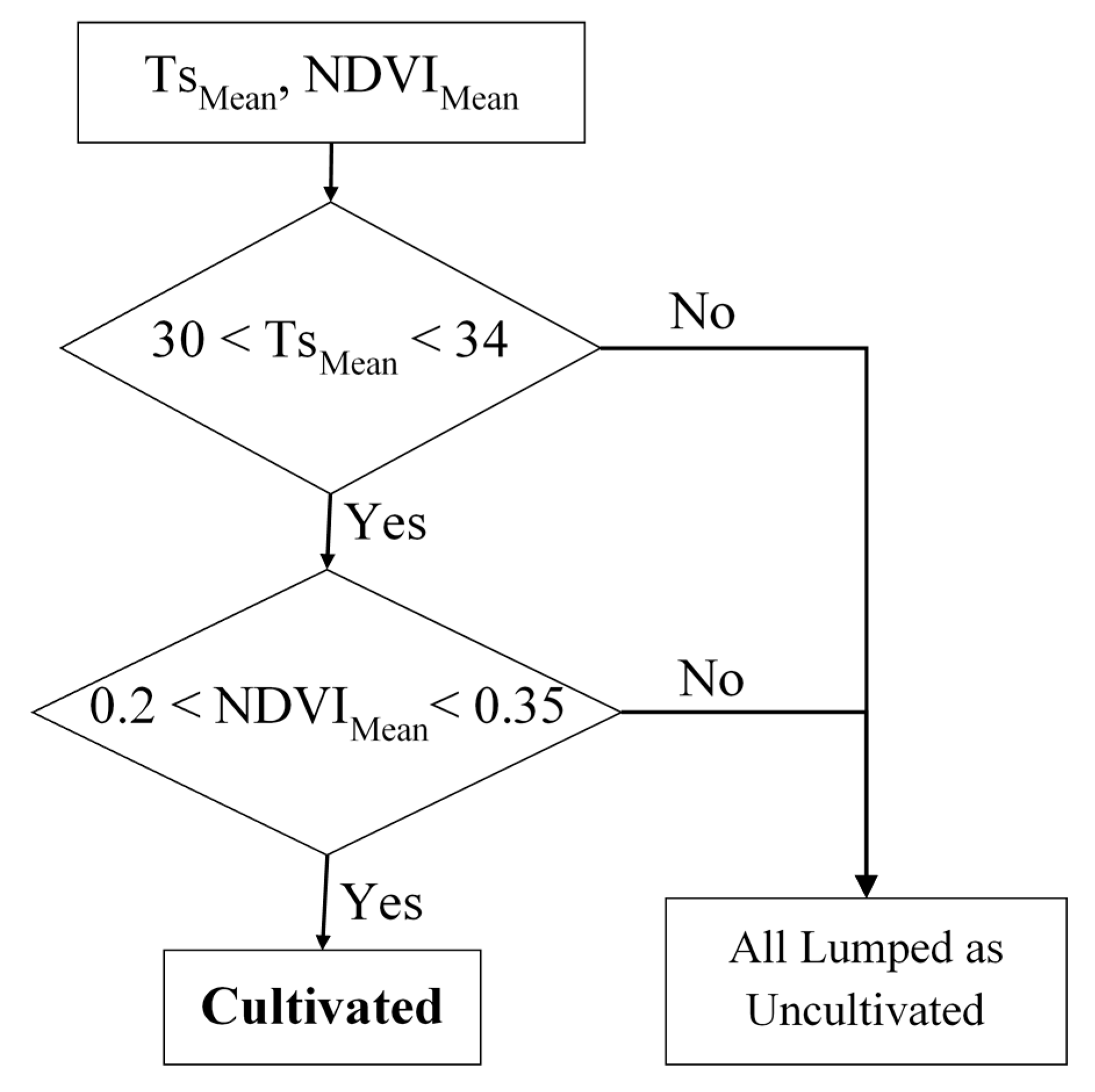
4.2. Building the Algorithm
4.3. Verification
5. Conclusions
Acknowledgments
Author Contributions
Conflicts of Interest
References
- Van Halsema, G.E.; Vincent, L. Efficiency and productivity terms for water management: A matter of contextual relativism versus general absolutism. Agric. Water Manag. 2012, 108, 9–15. [Google Scholar] [CrossRef]
- Haouari, M.; Azaiez, M.N. Optimum cropping patterns under water deficits: Theory and methodology. Eur. J. Oper. Res. 2001, 130, 133–146. [Google Scholar] [CrossRef]
- Salmona, J.M.; Friedla, M.A.; Frolking, S.; Wisser, D.; Douglas, E.M. Global rain-fed, irrigated, and paddy croplands: A new high resolution map derived from remote sensing, crop inventories and climate data. Int. J. Appl. Earth Obs. Geoinf. 2015, 38, 321–334. [Google Scholar] [CrossRef]
- Alexandridis, T.K.; Panagopoulos, A.; Galanis, G.; Alexia, I.; Cherif, I.; Chemin, Y.; Stavrinos, E.; Bilas, G.; Zalidis, G.C. Combining remotely sensed surface energy fluxes and GIS analysis of groundwater parameters for irrigation system assessment. Irrig. Sci. 2014, 32, 127–140. [Google Scholar] [CrossRef]
- Bastiaanssen, W.G.M.; Molden, D.J.; Makin, I.W. Remote sensing for irrigated agriculture: Examples from research and possible applications. Agric. Water Manag. 2000, 46, 137–155. [Google Scholar] [CrossRef]
- Ambast, S.K.; Keshari, A.K.; Gosain, A.K. Satellite Remote Sensing to Support Management of Irrigation Systems: Concepts and Approaches. Irrig. Drain. 2002, 51, 25–39. [Google Scholar] [CrossRef]
- Atzberger, C. Advances in remote sensing of agriculture: Context description, existing operational monitoring systems and major information needs. Remote Sens. 2013, 5, 949–981. [Google Scholar] [CrossRef]
- Mondal, S.; Jeganathan, C.; Sinha, N.K.; Rajan, H.; Roy, T.; Kumar, P. Extracting seasonal cropping patterns using multi-temporal vegetation indices from IRS LISS-III data in Muzaffarpur district of Bihar, India. Egypt. J. Remote Sens. Space Sci. 2014, 17, 123–134. [Google Scholar] [CrossRef]
- Bastiaanssen, W.G.M.; Bos, M.G. Irrigation performance indicators based on remotely sensed data: A review of literature. Irrig. Drain. Syst. 1999, 13, 291–311. [Google Scholar] [CrossRef]
- Dadhwal, V.; Singh, R.; Dutta, S.; Parihar, J. Remote sensing based crop inventory: A review of Indian experience. Trop. Ecol. 2002, 43, 107–122. [Google Scholar]
- Schmedtmann, J.; Campagnolo, M.L. Reliable Crop Identification with Satellite Imagery in the Context of Common Agriculture Policy Subsidy Control. Remote Sens. 2015, 7, 9325–9346. [Google Scholar] [CrossRef]
- Bastiaanssen, W.G.M.; Ali, S. A new crop yield forecasting model based on satellite measurements applied across the Indus Basin, Pakistan. Agric. Ecosyst. Environ. 2003, 94, 321–340. [Google Scholar] [CrossRef]
- Lobell, D.B. The use of satellite data for crop yield gap analysis. Field Crops Res. 2013, 143, 56–64. [Google Scholar] [CrossRef]
- Singh, R.K.; Liu, S.; Tieszen, L.L.; Suyker, A.E.; Verma, S.B. Estimating seasonal evapotranspiration from temporal satellite images. Irrig. Sci. 2012, 30, 303–313. [Google Scholar] [CrossRef]
- Liou, Y.; Kar, S.K. Evapotranspiration Estimation with Remote Sensing and Various Surface Energy Balance Algorithms—A Review. Energies 2014, 7, 2821–2849. [Google Scholar] [CrossRef]
- Biggs, T.W.; Thenkabail, P.S.; Gumma, M.K.; Scott, C.A.; Parthasaradhi, G.R.; Turral, H.N. Irrigated area mapping in heterogeneous landscapes with MODIS time series, ground truth and census data, Krishna Basin, India. Int. J. Remote Sens. 2006, 27, 4245–4266. [Google Scholar] [CrossRef]
- Alexandridis, T.K.; Zalidis, G.C.; Silleos, N.G. Mapping irrigated area in Mediterranean basing using low cost satellite Earth Observation. Comput. Electron. Agric. 2008, 64, 93–103. [Google Scholar] [CrossRef]
- Pervez, M.S.; Brown, J.F. Mapping Irrigated Lands at 250-m Scale by Merging MODIS Data and National Agricultural Statistics. Remote Sens. 2010, 2, 2388–2412. [Google Scholar] [CrossRef]
- Gumma, M.K.; Thenkabail, P.S.; Hideto, F.; Nelson, A.; Dheeravath, V.; Busia, D.; Rala, A. Mapping Irrigated Areas of Ghana Using Fusiion of 30 m and 250 m Resolution of Remote-Sensing Data. Remote Sens. 2011, 3, 816–835. [Google Scholar] [CrossRef]
- Pervez, M.S.; Budde, M.; Rowland, J. Mapping irrigated areas in Afghanistan over the past decade using MODIS NDVI. Remote Sens. Environ. 2014, 149, 155–165. [Google Scholar] [CrossRef]
- Gallego, F.J.; Kussul, N.; Skakunb, S.; Kravchenko, O.; Shelestov, A.; Kussul, O. Efficiency assessment of using satellite data for crop area estimation in Ukraine. Int. J. Appl. Earth Obs. Geoinf. 2014, 29, 22–30. [Google Scholar] [CrossRef]
- Ozdogan, M.; Yang, Y.; Allez, G.; Cervantes, C. Remote Sensing of Irrigated Agriculture: Opportunities and challenges. Remote Sens. 2010, 2, 2274–2304. [Google Scholar] [CrossRef]
- Nemani, K.; Running, S. Land cover characterization using multitemporal red, near-IR and thermal-IR data from NOAA/AVHRR. Ecol. Appl. 1997, 7, 79–90. [Google Scholar] [CrossRef]
- Lambin, E.F.; Ehrlich, D. The surface temperature-vegetation index space for land cover and land-cover change analysis. Int. J. Remote Sens. 1996, 17, 463–487. [Google Scholar] [CrossRef]
- Karnieli, A.; Agam, N.; Pinker, R.T.; Anderson, M.; Imhoff, M.L.; Gutman, G.G.; Panov, N.; Goldberg, A. Use of NDVI and Land Surface Temperature for Drought Assessment: Merits and Limitations. J. Clim. 2010, 23, 618–633. [Google Scholar] [CrossRef]
- Julien, Y.; Sobrino, J.A.; Mattar, C.; Ruescas, A.B.; Jiménez-Muñoz, J.C.; Sòria, G.; Hidalgo, V.; Atitar, M.; Franch, B.; Cuenca, J. Temporal analysis of normalized difference vegetation index (NDVI) and land surface temperature (LST) parameters to detect changes in the Iberian land cover between 1981 and 2001. Int. J. Remote Sens. 2011, 32, 2057–2068. [Google Scholar] [CrossRef]
- Sinha, S.; Sharma, L.K.; Nathawat, M.S. Improved Land-use/Land-cover classification of semi-arid deciduous forest landscape using thermal remote sensing. Egypt. J. Remote Sens. Space Sci. 2015, 18, 217–233. [Google Scholar]
- Bashier, E.E.; Adeeb, A.M.; Ahmed, H.M. Assessment of water users associations in Spate Irrigation Systems: Case Study of Gash Delta Agricultural Corporation, Sudan. Int. J. Sudan Res. 2014, 4, 109–126. [Google Scholar]
- Swan, C. The Recorded Behaviour of the River Gash in Sudan; Ministry of Irrigation and Hydro-electric Power: Khartoum, Sudan, 1959.
- Anderson, I.M. The Easter Sudan Rehabilitation and Development Fund: GAS Phase II-Design Mission; Technical Paper on Main Findings and Recommendations; The Easter Sudan Rehabilitation and Development Fund (ESRDF): Kassala, Sudan, 2011. [Google Scholar]
- Chander, G.; Markham, B.L.; Helder, D.L. Summary of current radiometric calibration coefficients for Landsat MSS, TM, ETM+, and EO-1 ALI sensors. Remote Sens. Environ. 2009, 113, 893–903. [Google Scholar] [CrossRef]
- Xu, H. Modification of normalized difference water index to enhance open water features in remotely sensed imagery. Int. J. Remote Sens. 2006, 27, 3025–3033. [Google Scholar] [CrossRef]
- Koutsias, N. An autologistic regression model for increasing the accuracy of burned surface mapping using Landsat Thematic Mapper data. Int. J. Remote Sens. 2003, 24, 2199–2204. [Google Scholar] [CrossRef]


| Method of Estimation | Cultivated Area (ha) | ||||
|---|---|---|---|---|---|
| Kassala | Mekali | Degain | Tendelai | Metateib | |
| Field report | 5064 | 4876 | 5621 | 5371 | 2924 |
| Remote sensing | 4954 | 4648 | 5845 | 5330 | 3286 |
| Error (ha) | −110 | −228 | 224 | −41 | 362 |
| Error (%) | −2 | −5 | 4 | −1 | 12 |
| Method of Estimation | Cultivated Area (ha) | ||||
|---|---|---|---|---|---|
| Kassala | Mekali | Degain | Tendelai | Metateib | |
| Field report | 4066 | 3459 | 5397 | 1806 | 2054 |
| Remote sensing | 4485 | 4156 | 4746 | 1471 | 1532 |
| Error (ha) | 419 | 697 | −651 | −335 | −522 |
| Error (%) | 10 | 20 | −12 | −19 | −25 |
© 2018 by the authors. Licensee MDPI, Basel, Switzerland. This article is an open access article distributed under the terms and conditions of the Creative Commons Attribution (CC BY) license (http://creativecommons.org/licenses/by/4.0/).
Share and Cite
Ghebreamlak, A.Z.; Tanakamaru, H.; Tada, A.; Ahmed Adam, B.M.; Elamin, K.A.E. Satellite-Based Mapping of Cultivated Area in Gash Delta Spate Irrigation System, Sudan. Remote Sens. 2018, 10, 186. https://0-doi-org.brum.beds.ac.uk/10.3390/rs10020186
Ghebreamlak AZ, Tanakamaru H, Tada A, Ahmed Adam BM, Elamin KAE. Satellite-Based Mapping of Cultivated Area in Gash Delta Spate Irrigation System, Sudan. Remote Sensing. 2018; 10(2):186. https://0-doi-org.brum.beds.ac.uk/10.3390/rs10020186
Chicago/Turabian StyleGhebreamlak, Araya Z., Haruya Tanakamaru, Akio Tada, Bashir M. Ahmed Adam, and Khalid A. E. Elamin. 2018. "Satellite-Based Mapping of Cultivated Area in Gash Delta Spate Irrigation System, Sudan" Remote Sensing 10, no. 2: 186. https://0-doi-org.brum.beds.ac.uk/10.3390/rs10020186