Estimating Barley Biomass with Crop Surface Models from Oblique RGB Imagery


Institute of Geography, GIS & RS Group, University of Cologne, 50923 Cologne, Germany
*
Author to whom correspondence should be addressed.
Remote Sens. 2018, 10(2), 268; https://0-doi-org.brum.beds.ac.uk/10.3390/rs10020268
Submission received: 20 November 2017
/
Revised: 15 January 2018
/
Accepted: 7 February 2018
/
Published: 9 February 2018
(This article belongs to the Special Issue Estimation of Crop Phenotyping Traits using Unmanned Ground Vehicle and Unmanned Aerial Vehicle Imagery)
Abstract
:Non-destructive monitoring of crop development is of key interest for agronomy and crop breeding. Crop Surface Models (CSMs) representing the absolute height of the plant canopy are a tool for this. In this study, fresh and dry barley biomass per plot are estimated from CSM-derived plot-wise plant heights. The CSMs are generated in a semi-automated manner using Structure-from-Motion (SfM)/Multi-View-Stereo (MVS) software from oblique stereo RGB images. The images were acquired automatedly from consumer grade smart cameras mounted at an elevated position on a lifting hoist. Fresh and dry biomass were measured destructively at four dates each in 2014 and 2015. We used exponential and simple linear regression based on different calibration/validation splits. Coefficients of determination between 0.55 and 0.79 and root mean square errors (RMSE) between 97 and 234 g/m2 are reached for the validation of predicted vs. observed dry biomass, while Willmott’s refined index of model performance ranges between 0.59 and 0.77. For fresh biomass, values between 0.34 and 0.61 are reached, with root mean square errors (RMSEs) between 312 and 785 g/m2 and between 0.39 and 0.66. We therefore established the possibility of using this novel low-cost system to estimate barley dry biomass over time.
1. Introduction
The non-destructive monitoring of crop development and determination of crop traits is of key interest in agronomy and crop breeding, and efforts to estimate biomass from ground-based non-destructive measurements have been undertaken since the 1980s [1]. Since it is proven that, e.g., plant height, chlorophyll, and biomass, can be robustly determined with imaging from Unmanned Aerial Vehicles (UAVs) [2,3], the potential of UAV-based imaging for phenotyping is obvious [4,5]. The key data analysis technologies in this context are: (i) Structure-from-Motion (SfM) providing Digital Surface Models (DSMs) and RGB-, multi- or hyperspectral orthophotos; and (ii) the analysis of the multitemporal DSMs according to the approach of Crop Surface Models (CSMs) [6,7,8]. LiDAR is another technology that allows the derivation of DSMs. Studies that successfully used UAV- or LiDAR-derived DSMs for vegetation monitoring include [9,10,11,12,13].
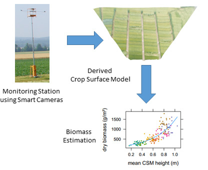
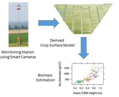
Andrade-Sanchez et al. [14] state that “Perhaps the greatest challenge for plant breeding and genetics research in the 21st century is establishing the capacity for rapidly and accurately phenotyping vast numbers of field-grown plants”. In crop breeding and phenotyping, data acquisition in very high temporal resolution (daily) is essential for certain phenological stages (e.g., emergence) and the evaluation and selection of best-performing cultivars [14]. Großkinsky et al. [15] summarize that the systems must be cost-effective and robust and that UAVs are providing increasing potential for multi-temporal data acquisition. However, the usage of UAVs might be limited due to weather, infrastructure, or technical restrictions. Besides, in plant breeding, the aerial coverage of the experimental plots and the total area is rather small. Hence, the installation of a cost-effective continuously operating monitoring station has the advantage of delivering daily imagery to derive certain crop traits. For this purpose, Brocks et al. [16] introduced a static low-cost 3D crop-monitoring system which acquires oblique stereo imagery from consumer grade smart cameras for deriving the crop trait plant height. As the authors proved, this system enables the non-destructive determination of plant height in different phenological stages, and the monitoring quality almost equals UAV-based approaches.
Building upon that system, the overall objective of this research is to evaluate the suitability of the static crop-monitoring system by using data derived in two growing seasons for estimating additional crop traits: dry and fresh biomass of barley. The use of plant height as a predictor for deriving crop biomass is well-established, both for UAV- and LiDAR-based data acquisition [2,17,18,19] as well as with in-situ measurements [20]. In this study, the CSM-derived plant heights, generated from the oblique stereo RGB imagery, are investigated to validate the potential and the robustness of the newly introduced 3D monitoring system to estimate biomass during plant growth.
2. Materials and Methods
2.1. Study Site
This study was carried out at Campus Klein-Altendorf (50°37′27″N, 6°59′16″E), the experimental campus of the agricultural faculty of the University of Bonn. For the growing periods of 2014 and 2015, a summer barley field experiment was set up where nine barley cultivars were cultivated with two different nitrogen treatments (40 and 80 kg N/ha) in three repetitions. The experiment was set up at separate locations on the experimental campus for 2014 and 2015, thus preventing issues with autocorrelation from measuring at the same location across years, as can be seen in Figure 1. Fifty-four plots were planted using a seeding density of 300 plants/m2 and a row spacing of 0.104 m. The plots had a size of 3 by 7 m, with each plot being divided into two parts, a 3 by 2 m area where the destructive biomass measurements were carried out and a 3 by 5 m area for all other non-destructive measurements. The day of seeding for the 2014 field experiment was 13 March 2014. For the 2015 field experiment, the plots were seeded on 23 March 2015.
2.2. Plant Height and Biomass Measurements
Dry and fresh biomass, as well as plant height, were determined for a selection of six of the nine cultivars at four dates per growing period (56, 70, 84 and 96 days after seeding (DAS) for 2014 and 55, 67, 83 and 97 DAS for 2015). The determination of cultivars to be used for biomass sampling was made not only for this study, but in cooperation with other studies carried out on the same field experiments. For the destructive biomass sampling, at each of the sample dates, all plants within a separate area of 0.04 m2 inside the destructive measurement area were extracted. After clipping the plants’ roots, the plants were cleaned. For the determination of fresh biomass, leaves and ears were weighed separately on the same day. The samples were dried for 120 h at 70 °C to obtain the dry biomass. After that, the plant organs were again weighed separately. Finally, the obtained weights were rescaled to g per m2. Dry biomass values for the last measurement date of 2015 were not available due to a problem in the lab. For the manual plant height measurements, the maximum standing height of the leaves or ears of 10 plants per plot was measured using a ruler with a precision of 1 cm and then averaged for each plot. At each measurement date, the growing stage in each plot was determined for three representative plants using the BBCH (Biologische Bundesanstalt, Bundessortenamt und CHemische Industrie) scale [21].
2.3. Crop Surface Models Derived Using Structure-from-Motion
CSMs are a tool for the multi-temporal monitoring of crop growth patterns and have been introduced as such by Hoffmeister et al. [6]. They can be created from different types of sensors such as LiDAR or RGB cameras using SfM [22] and Multi-View-Stereo (MVS) [23] techniques. In this study, the crop monitoring system presented in [16] was used to generate three CSMs per day during the growing seasons of 2014 and 2015. It uses a pair of smart cameras mounted in an elevated position to acquire oblique RGB imagery of the observed field. The RGB images are processed into 2.5D CSMs that represent the canopy surface using a combination of the commercial SfM/MVS software package Agisoft Photoscan (St. Petersburg, Russia) version 1.2.6 and the GIS software package Esri ArcGIS (Redlands, CA, USA) version 10.5. The quality setting “high” was used for the generation of the point clouds, as that resulted in best results in [16]. The points clouds were interpolated to a raster surface using the Inverse Distance Weighted (IDW) algorithm with a target cell size of 1 cm. The CSMs are georeferenced through ground control points (GCPs). The positions of the GCPs were also determined using the TopCon DGPS system. The process is semi-automated: the manual detection and marking of GCPs is the only manual processing step. A ground elevation raster was created by interpolating from the X/Y/Z coordinates of the plot corners as determined by measuring them with the highly accurate TopCon (Tokyo, Japan) HiPer Pro DGPS system [24]. By subtracting that ground elevation raster from the interpolated CSM, we can derive a raster that represents the height of the plants above the ground surface. For each plot, the borders of the plot areas marked for non-destructive measurements (cf. Figure 1) were buffered by 30 cm to eliminate possible border effects. Zonal statistics were used to calculate the mean CSM height per plot by using the buffered plot outlines as zone borders.
2.4. Statistical Analysis
The statistical analysis including correlation and regression was performed using R version 3.4.1. Manually measured mean plant height per plot was compared to the mean plant height per plot in the corresponding plant height raster. For each manual sampling date, one CSM was chosen out of all the CSMs generated on the day of the manual sampling date and the preceding and following day. We chose the CSM that covered the most plots of the six selected cultivars with a point density of at least 150 points/m2. When multiple CSMs covered the same amount of plots, the CSMs with a higher mean point density were chosen.
On some dates of manual plant height and biomass measurements, CSMs were not available due to technical issues with the lifting hoist. For these dates, the CSMs of the closest date where CSMs were available were used. The quality of the CSMs derived using the three acquisition times was evaluated by performing a linear regression between the mean manually measured plant height per plot and the mean height per plot derived from the CSMs.
The dataset was split into calibration and validation parts to be able to predict biomass from the CSM-derived plant heights. Multiple splits of the dataset were considered:
- using two replications for calibration and one for validation;
- using one year for calibration and the other for validation; and
- randomly splitting the dataset 70%/30% and using the 70% part for calibration and the 30% part for validation 10,000 times and averaging the results.
We chose to consider these different split-strategies for several reasons. Using the first approach, i.e., the different replications for validation and calibration, was the most natural choice at first glance. Because the replications are not in random places across the field but grouped, the number of plots contained in each CSM varies per replication due to the different distances to the camera (cf. Figure 1). Therefore, varying results were expected between the replication combinations. The second approach, splitting across years, was performed to investigate the quality of the prediction of biomass across years. For more non-specific results, we chose the third approach, which was to perform a repeated 70%/30% split.
Using the calibration parts of the dataset, multiple regression models were established to estimate biomass. We investigated both fresh and dry biomass, used linear as well as exponential regression, and considered the whole growing period and only those dates where anthesis of the barley plants had not yet started, i.e., where the BBCH values were lower than 60. In effect, this excluded the values from both years’ last measurement date. For the linear regressions, a simple linear regression was calculated to predict dry or fresh biomass based on the CSM-derived plant heights. For the exponential regressions, the measured fresh and dry biomass values were natural-log transformed before performing the linear regression.
We calculated the coefficient of determination , and the root mean square error (RMSE) for the calibration of plant height vs. dry and fresh biomass. Cross-validation was performed using the validation parts of the dataset by performing a linear regression of actually measured biomass against the predicted biomass using the regression models established beforehand. For the exponential regressions, the estimated biomass can be derived from the estimated log-transformed value by retransformation. During this retransformation, a correction factor of according to [25] where equals the standard deviation of the residual was applied to avoid prediction bias. To evaluate the validation (measured vs. predicted biomass), we calculated the , the RMSE, Willmott’s refined index of model performance [26] and the mean relative error of the prediction (calculated by dividing the absolute difference between measured and predicted biomass by the measured biomass and calculating the mean). Willmott’s refined index of model performance is a dimensionless indicator of model performance reaching from −1 to 1. It “indicates the sum of the magnitudes of the differences between the model-predicted and observed deviations about the observed mean relative to the sum of the magnitudes of the perfect-model ( = , for all i) and observed deviations about the observed mean” [26] and is calculated using the equation
where is the individual predictions, the individual observations and is the observed mean. Because it does not contain squared errors, it is less sensitive to a small number of large errors when compared to the Nash–Sutcliffe model efficiency.
3. Results
3.1. Plant Height Measurements
The crop-monitoring system produced CSMs for 95 acquisition times in the 2014 growing season and 129 acquisition times in the 2015 growing season. Table 1 shows the dates of biomass and manual plant height sampling where CSMs were generated and the number of plots per CSM. The CSMs chosen as the basis for the statistical analysis are highlighted in yellow.
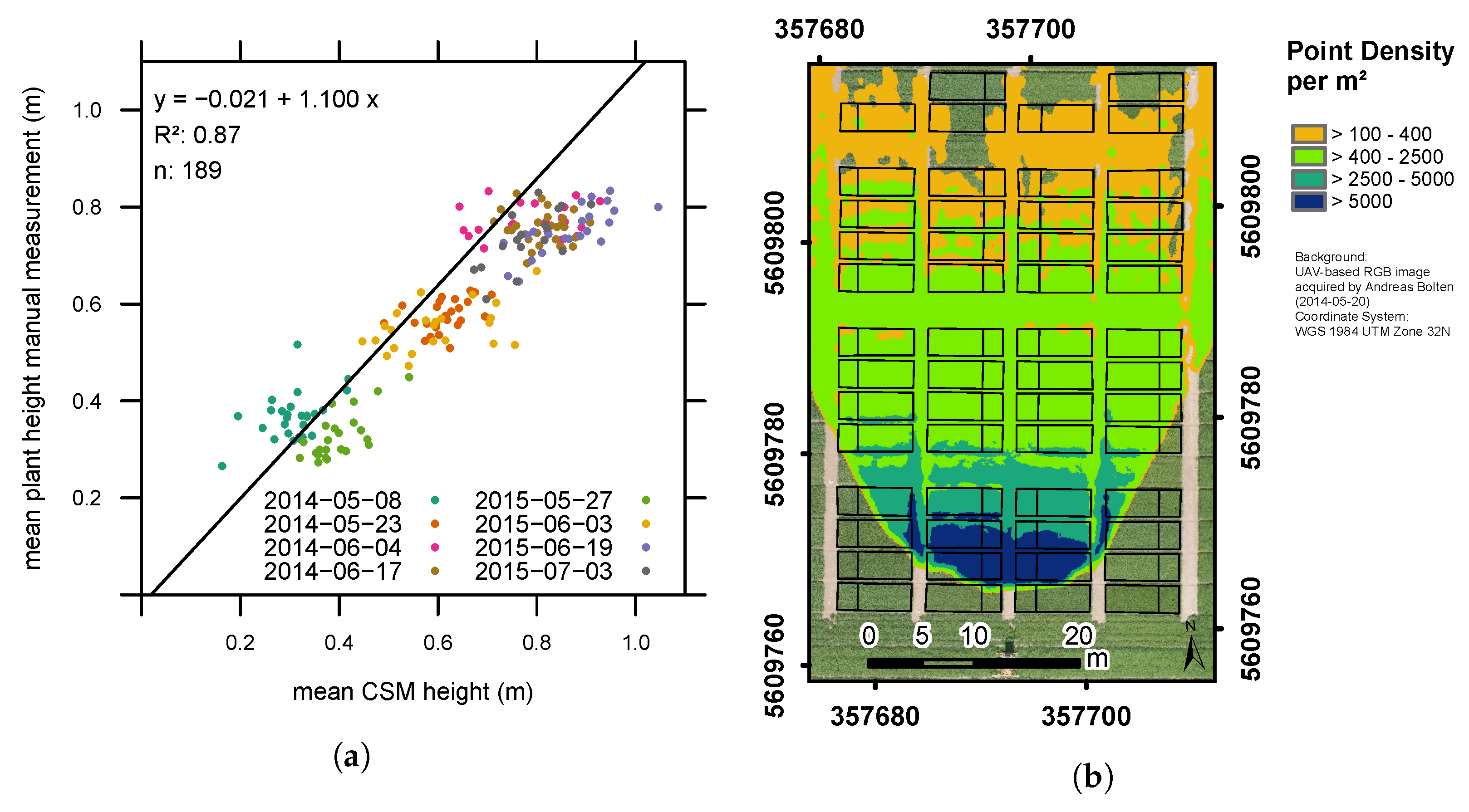
Table 2 shows the characteristics of the linear regressions that were performed between the CSM-derived plant height and the manually measured plant height using the selected CSMs for each acquisition time. Overall, high coefficients of determination > 0.8 were reached, confirming the validity of the CSM-derived plant heights, with an RMSE in the single-digit centimeter range. The noon acquisition time shows the highest and lowest RMSE as well as the joint-highest Willmott’s refined index of model performance [26] and thus the best result in estimating the real plant height when compared to the manual plant height measurements performed using a ruler. Therefore, we use the plant heights per plot derived from this acquisition date in the further statistical analysis and regression of plant height and biomass.
Figure 2a shows the linear regression between the CSM-derived plant heights of this noon acquisition time and the manual plant height measurements in a scatter plot. For the first measurement date of the 2014 growing season, the manually measured plant heights were higher than the corresponding CSM-derived plant heights. For all other dates, the CSM-derived plant heights are higher than the manually measured heights, especially for the measurement dates of the 2015 measurement campaign. This could be the case because the first measurement date in 2014 was earlier in the growing period than the first measurement date in 2015. Therefore, it is possible that ground pixels were included in the mean CSM-derived height per plot when the canopy was not yet completely closed. Within-date differences such as noted in [11] cannot be responsible, because we used the same time of day for all CSMs. Plant height increased over time across the vegetation periods until the measurement dates corresponding to the development of fruit in the BBCH scale (values ≥ 60) are reached.
Figure 2b shows the achieved point density and the parts of the experimental field that are covered by the generated CSM for the noon acquisition date of 8 May 2014. Only the plots that are visible in both cameras’ field of view are covered by the generated CSM (cf. Figure 1). We can see that the achieved point density decreased with increased distance to the cameras, which is expected due to the lower ground resolution associated with larger distances. This typical CSM shows that for the part of the field that was of primary interest, point densities higher than 400/m2 are achieved. We can also see that ca. 50% of the first repetition is typically not covered by the generated CSMs because of camera distance and field of view.
3.2. Biomass Estimation
Biomass was estimated based on ten different splits of the available data into calibration and verification datasets, for both dry and fresh biomass and using a simple linear regression of plant height and measured biomass, and a linear regression based on plant height and the natural log-transformed biomass, which is equivalent to an exponential regression.
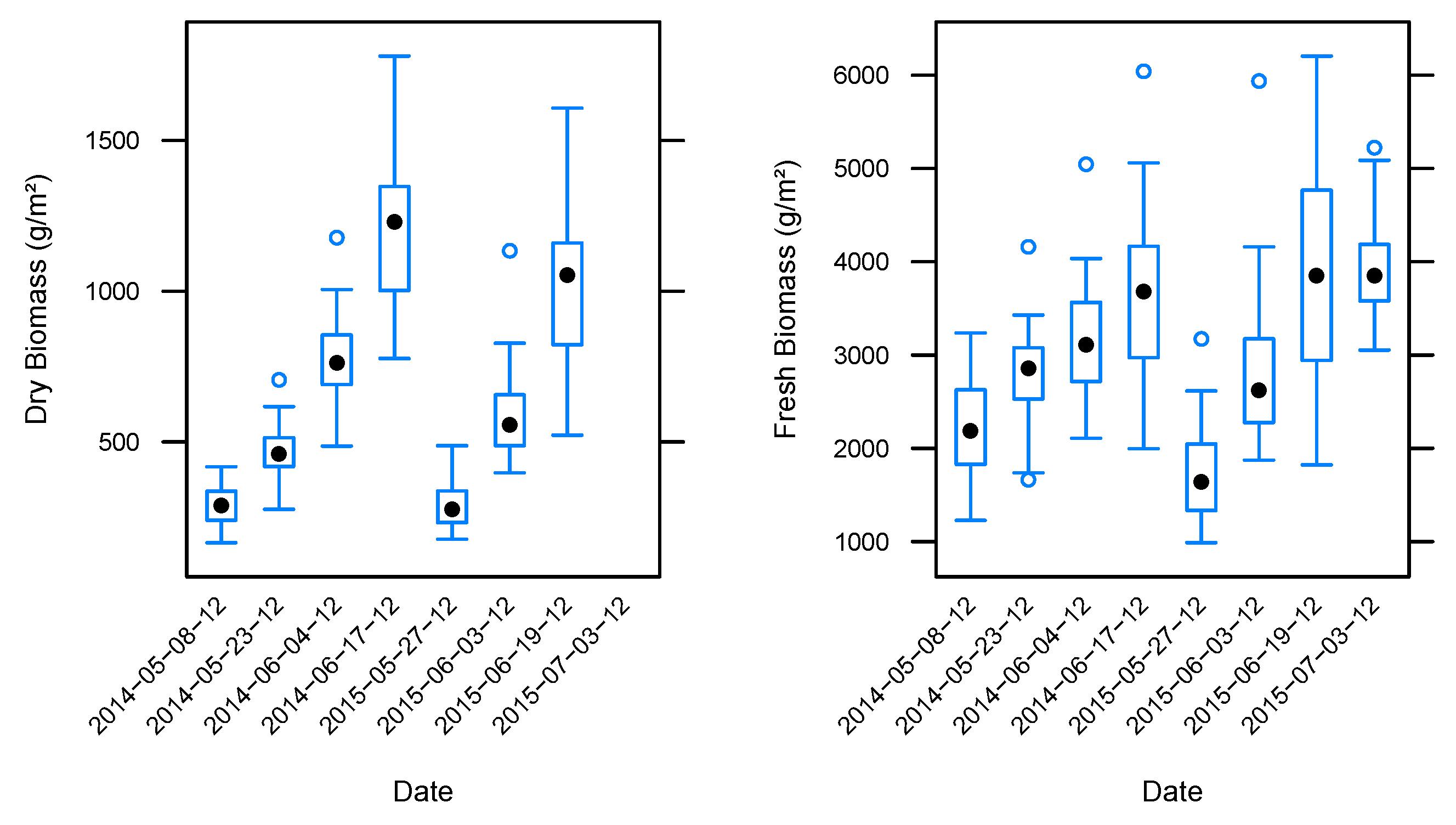
There is a higher variability in the fresh biomass values for each measuring date when compared to the dry biomass values, as can be seen in the boxplots in Figure 3. This suggests that plant water content varies considerably across the different plots for each measurement date.
We can look at the diagnostic plots for two exemplary regressions, one linear and one exponential for dry biomass, as shown in Figure 4, to examine whether the regression assumptions are met . We can see that the exponential regression models of CSM-derived plant height vs. dry biomass are a better fit for the data than the simple linear regression models: the residuals vs. fitted plot shows the difference between observed and predicted biomass plotted against the actual predicted biomass values. It shows more of a pattern for the linear regression, suggesting that the assumption of homoscedasticity is not fully met for the simple linear regressions. The normal Q–Q plot, which shows theoretical quantiles of a normal distribution plotted against quantiles of the residuals of the regression, allows us to evaluate the distribution of these residuals. In this case, it is closer to a normal distribution for the exponential regression by being closer to a diagonal line, showing that the normality assumption is met better by the exponential regressions. The scale-location plot, which plots the estimated biomass against the square root of the standardized residuals, shows that the residuals are spaced more evenly for the exponential regression, which is another sign that the assumption of homoscedasticity is met better by the exponential regressions. The residuals vs. leverage plots show that there are no overtly influential data points for both regressions: no data points are outside of Cook’s distance lines for either regression, and they are so far from the visible data points to not even be visible in the images.
Table 3 shows the details of the performed regressions. The estimation of dry biomass performs much better than that of fresh biomass, with values between 0.58 and 0.72 for the simple linear regression and values between 0.73 and 0.79 for the exponential regression. In contrast, the regression for the fresh biomass resulted in values between 0.36 and 0.59 for linear and 0.37 and 0.63 for the exponential regression. Looking at the dry biomass regression models and comparing the pre-anthesis regressions to the corresponding regressions for the whole growing period, it can be seen that pre-anthesis performs better with higher and lower RMSE, especially for the linear regression models. For fresh biomass, where all models perform worse than the corresponding dry biomass models, the difference between pre-anthesis and models based on data from the whole growing period is less pronounced. Of the exponential dry biomass models, only the of the model based on Repetitions 1 and 3 is more than one standard deviation higher than the mean of the 10,000 randomized 70%/30% models. Along with the model calibrated with the data of the 2015 measurements, is highest for both exponential and linear regression as well as the whole period and only the pre-anthesis period. For the fresh biomass, the difference between these two dataset partitions and the others is even more pronounced. The size of the calibration dataset does not appear to have a direct influence on the performance of the regressions.
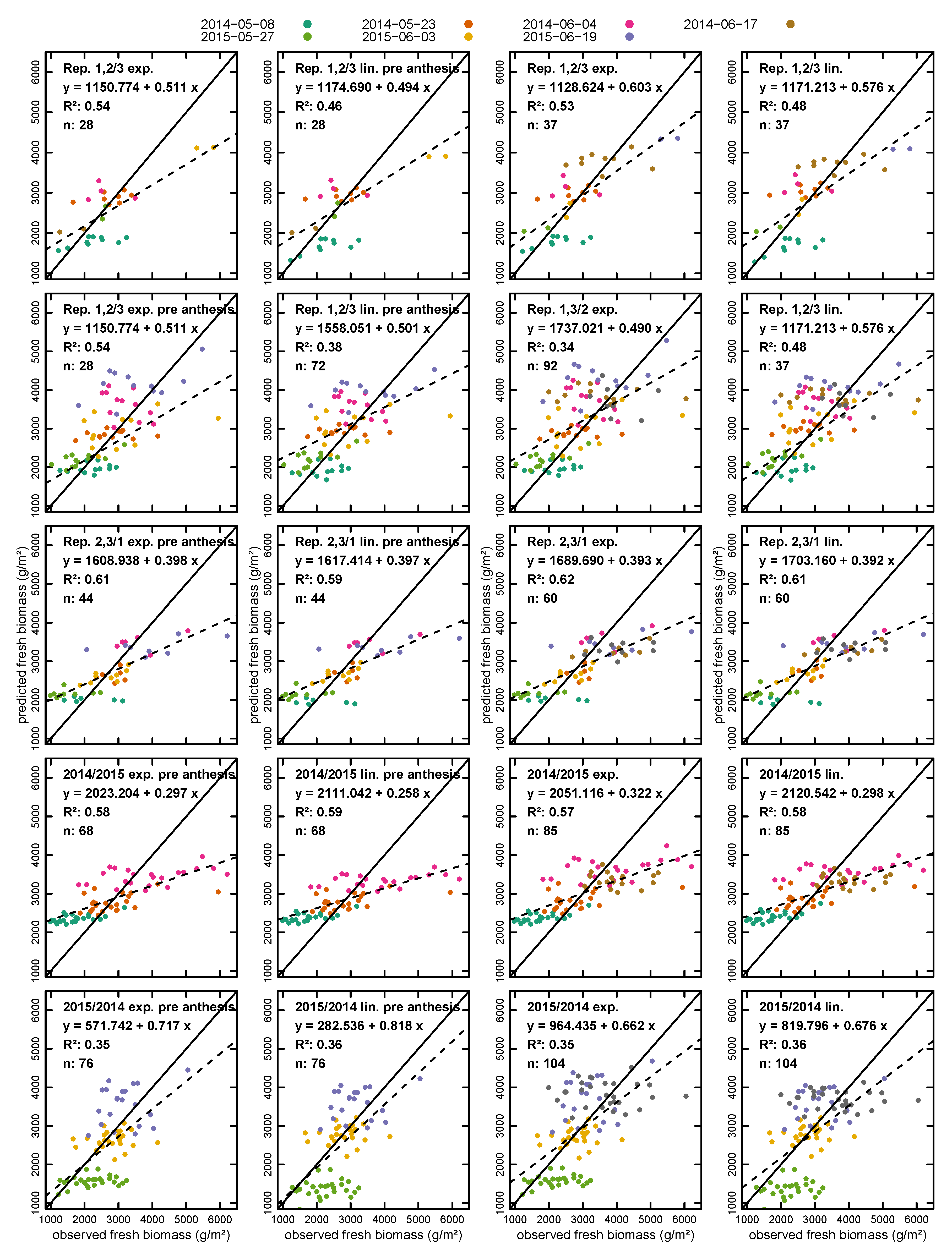
Figure 5 and Figure 6 graphically show observed vs. predicted dry and fresh biomass, respectively. Generally speaking, the fresh biomass validation shows bigger deviations of the slopes from the 1:1 line, indicating that dry biomass prediction works better than fresh biomass prediction. The regressions with slops closer to the 1:1 line, however, do not necessarily perform better, as measured by the and values.
The details of the cross-validation of the performed regressions are shown in Table 4. The models that show the best performance in the calibration, based on Repetitions 1 and 3 and the 2015 dataset and validated using Repetition 2 or the 2014 data, respectively, perform considerably worse here, with lower and higher RMSE values. Most of the models are within one standard deviation of the average quality parameters of the 10,000 repetitions of the 70%/30% split. The regressions with the lowest RMSE and relative error perform considerably better than the result of the repeated 70%/30% split, the possible reasons for this will be discussed later.
Figure 7 shows that, unlike the comparison along the growing season, for the single measurement dates, the relationship between dry biomass and mean CSM-derived plant height per plot is rather weak, confirming the results of [17]. Therefore, individual regression models for predicting biomass per date were not created.
4. Discussion
The effect the different acquisition dates have on the quality of the estimation of the plant height is most likely attributable to the effect of shadows in the acquired images. For the morning and evening acquisition times, the lower position of the sun results in more shadows within the photos, potentially reducing the quality of the derived point clouds due to the images having less contrast in shaded areas. The underestimation of plant height for the early measurement dates, when compared to the manual plant height measurements, is most likely caused by the fact that, for the early dates, ground pixels are still visible in the imagery which obviously lowers the height of the generated CSM due to the crop surface being a result of the interpolation between the generated 3D points.
The RMSE of derived plant height vs. the manually measured plant height of 8–9 cm (cf. Table 2) is comparable to the RMSE of derived plant height based on UAV or LiDAR measurements for other plants (e.g., 3.5 cm for LiDAR measurements on wheat [17], 10–13 cm for UAV-derived plant heights on poppy [18], and 10 cm for winter barley and wheat in [27]) and consistent with the measurements based on the 2014 field experiment presented in [16]. The RMSE of the calibration of the CSM-derived plant height vs. dry biomass regression is consistent if slightly higher when compared to the values achieved in [17] (112 g/m2 for LiDAR derived plant heights, and 115 g/m2 for SfM-derived plant heights). A better performance of LiDAR and UAV-derived heights is expected due to the higher accuracy of the LiDAR and the higher quality of the typically nadir images with consistent non-varying distance to the object acquired by an UAV.
As established in Figure 3, there is a higher variability in the fresh biomass values for each measuring date. Therefore, we keep our focus on discussing the dry biomass regression results.
The uneven performance of the regression models calibrated and validated by the different repetitions is most likely caused by the varying quality of the data over the replications. As can be seen in Figure 1, the plots belonging to Replication 1 are closest to the cameras and therefore have the highest point density, while Replication 3 is at the far end of the field from the cameras and therefore has the lowest point density, resulting in a worse estimation of plant height. By repeating the random 70%/30% split 10,000 times, the mean values for , RMSE and are most representative of the whole dataset.
Comparing the year-for-year regressions of the pre-anthesis data shows a similar result to the repeated randomized calibration/validation split, suggesting that the method presented is suitable for using a model derived from one year’s plant height data to predict dry biomass for the next year. Looking at the two year-for-year models for the whole vegetation period, using the 2015 data to predict the 2014 dry biomass has a worse result, which is most likely caused by the one measurement date late in the 2015 growing period where no dry biomass data were available.
Many studies have outlined the importance of non-spectral predictors such as plant height for non-destructive biomass estimation, with plant height being recorded by different sensors: manually in [20], using ultrasonic measurements in [28], using TLS and time-of-flight cameras in [29], and using TLS in [8]. Other studies derive plant height using UAV-captured imagery for crops such as barley [10], wheat [30] and sorghum [31] with a focus on field-phenotyping.
We can directly compare results for those studies that derived barley biomass from plant height, derived either from UAV-captured imagery [2,32] or TLS [8]. A comparison to the UAV-derived results shows that similar results are achieved. The coefficient of determination between predicted and observed dry biomass for the exponential regression is lower in our study for the whole vegetation period (0.63 vs. 0.8), but the RMSE and relative error are lower as well (185 g/m2 vs. 240 g/m2, 29.71% vs. 44.61%). Comparing the simple linear regression for the period excluding the anthesis also shows similar results ( 0.68 vs. 0.81, RMSE 135 g/m2 vs. 90 g/m2, and relative error 25.81% vs. 45.01%). The results of the study deriving barley biomass based on TLS plant height measurements [8] cannot be easily compared for the exponential regression models because Tilly et al. did not re-transform the log-transformed biomass values. Therefore, we can only compare the results of the simple linear regression. The prediction of dry biomass for the whole vegetation period achieved similar results ( of 0.63 vs. 0.66, RMSE of 177.29 g/m2 vs. 257.57 g/m2). In contrast, TLS performs slightly better for the pre-anthesis period ( of 0.68 vs. 0.8, RMSE 135.1 g/m2 vs. 147.75 g/m2).
5. Conclusions
The general goal of this study was to evaluate if the monitoring system presented by Brocks et al. [16] can be used as a robust and cost-effective means for estimating dry and fresh barley biomass on a per-plot scale. Towards this end, CSMs were generated in a semi-automated manner at daily time steps from oblique stereo RGB imagery using a combination of commercial SfM software and custom scripting. Considering that the system presented here is a low-cost system that allows semi-automated prediction during the whole vegetation period without extensive fieldwork for each measurement day, the results are outstanding.
There are other studies such as [33] that also use tower-based cameras for crop monitoring, in this case using RGB and NIR imagery for rice monitoring. Such spectral data could also be acquired using semi-automated smart cameras and then be combined with the CSM-derived plant heights for better biomass monitoring, comparable to the work done by Tilly et al. [8]. Other studies using this approach of combining spectral measures with plant height are, e.g., [2,20]. Another possibility for future work would be to investigate the possibility of a multi-station approach, merging the point clouds generated by cameras placed on multiple lifting hoists on opposite ends of the experimental field. Analogous to the approach usually employed in TLS, the drawback of reduced point density with increased camera distance could be compensated if it is possible to adequately merge the generated point clouds before the CSM is generated.
Acknowledgments
We acknowledge the staff of Campus Klein-Altendorf (University of Bonn) for managing the field experiment as well as providing the hydraulic lifting hoist and the mounting platform for the cameras. The field experiment was setup within the CROP.SENSe.net project in the context of the Ziel 2-Programm NRW 2007–2013 “Regionale Wettbewerbsfähigkeit und Beschäftigung” by the Ministry for Innovation, Science and Research (MIWF) of the state North Rhine Westphalia (NRW) and European Union Funds for regional development (EFRE) (005-1103-0018).
Author Contributions
Sebastian Brocks and Georg Bareth conceived and designed the experiments; Sebastian Brocks performed the experiments; Sebastian Brocks analyzed the data; and Sebastian Brocks and Georg Bareth wrote the paper.
Conflicts of Interest
The authors declare no conflict of interest.
References
- Bouman, B.A.M.; Goudriaan, J. Estimation of crop growth from optical and microwave soil cover. Int. J. Remote Sens. 1989, 10, 1843–1855. [Google Scholar] [CrossRef]
- Bendig, J.; Yu, K.; Aasen, H.; Bolten, A.; Bennertz, S.; Broscheit, J.; Gnyp, M.L.; Bareth, G. Combining UAV-based plant height from crop surface models, visible, and near infrared vegetation indices for biomass monitoring in barley. Int. J. Appl. Earth Obs. Geoinf. 2015, 39, 79–87. [Google Scholar] [CrossRef]
- Jay, S.; Gorretta, N.; Morel, J.; Maupas, F.; Bendoula, R.; Rabatel, G.; Dutartre, D.; Comar, A.; Baret, F. Estimating leaf chlorophyll content in sugar beet canopies using millimeter- to centimeter-scale reflectance imagery. Remote Sens. Environ. 2017, 198, 173–186. [Google Scholar] [CrossRef]
- Jin, X.; Liu, S.; Baret, F.; Hemerlé, M.; Comar, A. Estimates of plant density of wheat crops at emergence from very low altitude UAV imagery. Remote Sens. Environ. 2017, 198, 105–114. [Google Scholar] [CrossRef]
- Yang, G.; Liu, J.; Zhao, C.; Li, Z.; Huang, Y.; Yu, H.; Xu, B.; Yang, X.; Zhu, D.; Zhang, X.; et al. Unmanned Aerial Vehicle Remote Sensing for Field-Based Crop Phenotyping: Current Status and Perspectives. Front. Plant Sci. 2017, 8, 1111. [Google Scholar] [CrossRef] [PubMed]
- Hoffmeister, D.; Bolten, A.; Curdt, C.; Waldhoff, G.; Bareth, G. High-resolution Crop Surface Models (CSM) and Crop Volume Models (CVM) on field level by terrestrial laser scanning. Proc. SPIE 2010. [Google Scholar] [CrossRef]
- Aasen, H.; Burkart, A.; Bolten, A.; Bareth, G. Generating 3D hyperspectral information with lightweight UAV snapshot cameras for vegetation monitoring: From camera calibration to quality assurance. ISPRS J. Photogramm. Remote Sens. 2015, 108, 245–259. [Google Scholar] [CrossRef]
- Tilly, N.; Aasen, H.; Bareth, G. Fusion of Plant Height and Vegetation Indices for the Estimation of Barley Biomass. Remote Sens. 2015, 7, 11449–11480. [Google Scholar] [CrossRef]
- Lucieer, A.; Turner, D.; King, D.H.; Robinson, S.A. International Journal of Applied Earth Observation and Geoinformation Using an Unmanned Aerial Vehicle ( UAV ) to capture micro-topography of Antarctic moss beds. Int. J. Appl. Earth Obs. Geoinf. 2014, 27, 53–62. [Google Scholar] [CrossRef]
- Bendig, J.; Bolten, A.; Bareth, G. UAV-based Imaging for Multi-Temporal, very high Resolution Crop Surface Models to monitor Crop Growth Variability. Photogramm. Fernerkund. Geoinf. 2013, 6, 551–562. [Google Scholar] [CrossRef]
- Friedli, M.; Kirchgessner, N.; Grieder, C.; Liebisch, F.; Mannale, M.; Walter, A. Terrestrial 3D laser scanning to track the increase in canopy height of both monocot and dicot crop species under field conditions. Plant Methods 2016, 12, 9. [Google Scholar] [CrossRef] [PubMed]
- Bareth, G.; Bendig, J.; Tilly, N.; Hoffmeister, D.; Aasen, H.; Bolten, A. A Comparison of UAV- and TLS-derived Plant Height for Crop Monitoring: Using Polygon Grids for the Analysis of Crop Surface Models (CSMs). Photogramm. Fernerkund. Geoinf. 2016, 2016, 85–94. [Google Scholar] [CrossRef]
- Geipel, J.; Link, J.; Claupein, W. Combined Spectral and Spatial Modeling of Corn Yield Based on Aerial Images and Crop Surface Models Acquired with an Unmanned Aircraft System. Remote Sens. 2014, 11, 10335–10355. [Google Scholar] [CrossRef]
- Andrade-Sanchez, P.; Gore, M.A.; Heun, J.T.; Thorp, K.R.; Carmo-Silva, E.; French, A.N.; Salvucci, M.E.; White, J.W. Development and evaluation of a field-based high-throughput phenotyping platform. Funct. Plant Biol. 2014, 41, 68–79. [Google Scholar] [CrossRef]
- Großkinsky, D.K.; Pieruschka, R.; Svensgaard, J.; Rascher, U.; Christensen, S.; Schurr, U.; Roitsch, T. Phenotyping in the fields: Dissecting the genetics of quantitative traits and digital farming. New Phytol. 2015, 207, 950–952. [Google Scholar] [CrossRef] [PubMed]
- Brocks, S.; Bendig, J.; Bareth, G. Toward an automated low-cost three-dimensional crop surface monitoring system using oblique stereo imagery from consumer-grade smart cameras. J. Appl. Remote Sens. 2016, 10, 046021. [Google Scholar] [CrossRef]
- Madec, S.; Baret, F.; de Solan, B.; Thomas, S.; Dutartre, D.; Jezequel, S.; Hemmerlé, M.; Colombeau, G.; Comar, A. High-Throughput Phenotyping of Plant Height: Comparing Unmanned Aerial Vehicles and Ground LiDAR Estimates. Front. Plant Sci. 2017, 8, 2002. [Google Scholar] [CrossRef] [PubMed]
- Iqbal, F.; Lucieer, A.; Barry, K.; Wells, R. Poppy Crop Height and Capsule Volume Estimation from a Single UAS Flight. Remote Sens. 2017, 9, 647. [Google Scholar] [CrossRef]
- Tilly, N.; Hoffmeister, D.; Cao, Q.; Huang, S.; Lenz-Wiedemann, V.; Miao, Y.; Bareth, G. Multitemporal crop surface models: Accurate plant height measurement and biomass estimation with terrestrial laser scanning in paddy rice. J. Appl. Remote Sens. 2014, 8, 083671. [Google Scholar] [CrossRef]
- Marshall, M.; Thenkabail, P. Developing in situ non-destructive estimates of crop biomass to address issues of scale in remote sensing. Remote Sens. 2015, 7, 808–835. [Google Scholar] [CrossRef]
- Lancashire, P.D.; Bleiholder, H.; Van Den Boom, T.; Langelüddeke, P.; Stauss, R.; Weber, E.; Witzenberger, A. A uniform decimal code for growth stages of crops and weeds. Ann. Appl. Biol. 1991, 119, 561–601. [Google Scholar] [CrossRef]
- Ullman, S. The Interpretation of Structure from Motion. Proc. R. Soc. Lond. Ser. B 1979, 203, 405–426. [Google Scholar] [CrossRef]
- Seitz, S.; Curless, B.; Diebel, J.; Scharstein, D.; Szeliski, R. A Comparison and Evaluation of Multi-View Stereo Reconstruction Algorithms. In Proceedings of the 2006 IEEE Computer Society Conference on Computer Vision and Pattern Recognition (CVPR’06), New York, NY, USA, 17–22 June 2006; Volume 1, pp. 519–528. [Google Scholar]
- Topcon Positioning Systems Inc. HiPer Pro Operator’s Manual. 2006. Available online: https://www.servicestopni.com/resources/top-survey/downloads/HiPerPro_om.pdf (accessed on 8 February 2018).
- Newman, M.C. Regression analysis of log-transformed data: Statistical bias and its correction. Environ. Toxicol. Chem. 1993, 12, 1129–1133. [Google Scholar] [CrossRef]
- Willmott, C.J.; Robeson, S.M.; Matsuura, K. A refined index of model performance. Int. J. Climatol. 2012, 32, 2088–2094. [Google Scholar] [CrossRef]
- Hoffmeister, D.; Waldhoff, G.; Korres, W.; Curdt, C.; Bareth, G. Crop height variability detection in a single field by multi-temporal terrestrial laser scanning. Precis. Agric. 2016, 17, 296–312. [Google Scholar] [CrossRef]
- Moeckel, T.; Safari, H.; Reddersen, B.; Fricke, T.; Wachendorf, M. Fusion of ultrasonic and spectral sensor data for improving the estimation of biomass in grasslands with heterogeneous sward structure. Remote Sens. 2017, 9, 98. [Google Scholar] [CrossRef]
- Hämmerle, M.; Höfle, B. Direct derivation of maize plant and crop height from low-cost time-of-flight camera measurements. Plant Methods 2016, 12, 50. [Google Scholar] [CrossRef] [PubMed]
- Holman, F.H.; Riche, A.B.; Michalski, A.; Castle, M.; Wooster, M.J.; Hawkesford, M.J. High throughput field phenotyping of wheat plant height and growth rate in field plot trials using UAV based remote sensing. Remote Sens. 2016, 8, 1031. [Google Scholar] [CrossRef]
- Watanabe, K.; Guo, W.; Arai, K.; Takanashi, H.; Kajiya-Kanegae, H.; Kobayashi, M.; Yano, K.; Tokunaga, T.; Fujiwara, T.; Tsutsumi, N.; et al. High-Throughput Phenotyping of Sorghum Plant Height Using an Unmanned Aerial Vehicle and Its Application to Genomic Prediction Modeling. Front. Plant Sci. 2017, 8, 421. [Google Scholar] [CrossRef] [PubMed]
- Bendig, J.; Bolten, A.; Bennertz, S.; Broscheit, J.; Eichfuss, S.; Bareth, G. Estimating Biomass of Barley Using Crop Surface Models (CSMs) Derived from UAV-Based RGB Imaging. Remote Sens. 2014, 6, 10395–10412. [Google Scholar] [CrossRef]
- Naito, H.; Ogawa, S.; Valencia, M.O.; Mohri, H.; Urano, Y.; Hosoi, F.; Shimizu, Y.; Chavez, A.L.; Ishitani, M.; Selvaraj, M.G.; et al. Estimating rice yield related traits and quantitative trait loci analysis under different nitrogen treatments using a simple tower-based field phenotyping system with modified single-lens reflex cameras. ISPRS J. Photogramm. Remote Sens. 2017, 125, 50–62. [Google Scholar] [CrossRef]
Figure 1.
Summer barley field experiment in 2014 and 2015.

Figure 2.
(a) Scatter plot of CSM-derived plant height vs. manually measured plant height for the selected CSMs of the noon acquisition date, p-value < 0.0001; and (b) overview of covered plots and point density per m2 for 8 May 2014, noon acquisition date.
Figure 2.
(a) Scatter plot of CSM-derived plant height vs. manually measured plant height for the selected CSMs of the noon acquisition date, p-value < 0.0001; and (b) overview of covered plots and point density per m2 for 8 May 2014, noon acquisition date.

Figure 3.
Boxplot of measured dry and fresh biomass values.

Figure 4.
Diagnostic plots for two exemplary regressions: (a) linear regression for Repetitions 1 and 2; and (b) exponential regression for Repetitions 1 and 2.
Figure 4.
Diagnostic plots for two exemplary regressions: (a) linear regression for Repetitions 1 and 2; and (b) exponential regression for Repetitions 1 and 2.

Figure 5.
Observed vs. predicted dry biomass. The solid line is the 1:1 line, and the dashed line is the regression line.
Figure 5.
Observed vs. predicted dry biomass. The solid line is the 1:1 line, and the dashed line is the regression line.

Figure 6.
Observed vs. predicted fresh biomass. The solid line is the 1:1 line, and the dashed line is the regression line.
Figure 6.
Observed vs. predicted fresh biomass. The solid line is the 1:1 line, and the dashed line is the regression line.

Figure 7.
Exponential regression of mean CSM-derived plant height per plot and dry biomass per measurement date.
Figure 7.
Exponential regression of mean CSM-derived plant height per plot and dry biomass per measurement date.


Table 1.
Overview of generated CSMs and corresponding BBCH values; selected CSMs highlighted.
| Date | Number of Plots with Point Density > 150/m2 (Average Point Density/m2 per Plot) | BBCH | ||
|---|---|---|---|---|
| Morning | Noon | Evening | ||
| 7 May 2014 (55 DAS) | * | n = 23 (991) | n = 25 (1412) | tillering–stem elongation (24–32) |
| 8 May 2014 (56 DAS) | n = 29 (1297) | n = 28 (1324) | n = 30 (1399) | |
| 9 May 2014 (57 DAS) | n = 29 (1271) | n = 17 (1064) | n = 28 (1029) | |
| 26 May 2015 (60 DAS) | * | * | n = 24 (2106) | tillering (21–27) |
| 27 May 2015 (61 DAS) | n = 24 (2077) | n = 23 (2271) | n = 23 (2461) | |
| 1 June 2015 (66 DAS) | n = 20 (1848) | n = 22 (2122) | n = 22 (2146) | booting (41–47) |
| 2 June 2015 (67 DAS) | n = 6 (509) | n = 22 (2143) | n = 10 (509) | |
| 3 June 2015 (68 DAS) | n = 23 (2743) | n = 23 (2451) | n = 22 (2319) | |
| 21 May 2014 (69 DAS) | n = 25 (1185) | n = 23 (1356) | n = 25 (1224) | booting (47–49) |
| 22 May 2014 (70 DAS) | n = 22 (1222) | n = 20 (1443) | n = 17 (1785) | |
| 23 May 2014 (71 DAS) | n = 20 (1368) | n = 26 (1222) | n = 24 (1244) | |
| 17 June 2015 (82 DAS) | n = 22 (2298) | n = 17 (1377) | n = 23 (1608) | inflorescence emergence, heading (51–59) |
| 18 June 2015 (83 DAS) | n = 17 (1415) | n = 21 (1593) | n = 18 (1214) | |
| 19 June 2015 (84 DAS) | n = 16 (944) | n = 22 (1683) | n = 23 (2004) | |
| 4 June 2014 (83 DAS) | n = 26 (1145) | n = 22 (1297) | n = 11 (1136) | inflorescence emergence, heading (52–59) |
| 5 June 2014 (84 DAS) | * | n = 12 (1186) | n = 20 (1267) | |
| 16 June 2014 (95 DAS) | n = 28 (1462) | n = 23 (1404) | n = 27 (1277) | development of fruit (71–75) |
| 17 June 2014 (96 DAS) | n = 27 (1351) | n = 28 (1397) | n = 27 (1407) | |
| 18 June 2014 (97 DAS) | n = 28 (1299) | n = 24 (1061) | n = 27 (1269) | |
| 1 July 2015 (96 DAS) | * | n = 17 (2727) | n = 17 (3108) | development of fruit (73–75) |
| 2 July 2015 (97 DAS) | n = 17 (2159) | n = 17 (1810) | n = 18 (1824) | |
| 3 July 2015 (98 DAS) | n = 17 (3337) | n = 17 (3350) | n = 18 (2016) | |
* no CSM available.
Table 2.
Statistics for the linear regression of CSM-derived and manual height per plot for the three acquisition times of the selected CSMs. : coefficient of determination; RMSE: root mean square error; : Willmott’s refined index of model performance [26]. p-Value < 0.0001 for all regressions.
Table 2.
Statistics for the linear regression of CSM-derived and manual height per plot for the three acquisition times of the selected CSMs. : coefficient of determination; RMSE: root mean square error; : Willmott’s refined index of model performance [26]. p-Value < 0.0001 for all regressions.
| Acquisition Time | RMSE (m) | ||
|---|---|---|---|
| morning (n = 194) | 0.81 | 0.09 | 0.77 |
| noon (n = 189) | 0.87 | 0.08 | 0.77 |
| evening (n = 189) | 0.81 | 0.09 | 0.75 |
Table 3.
Statistics of model calibration for regression of CSM-derived plant height against biomass, ncal: number of samples in calibration dataset; : coefficient of determination; RMSE: root mean square error.
Table 3.
Statistics of model calibration for regression of CSM-derived plant height against biomass, ncal: number of samples in calibration dataset; : coefficient of determination; RMSE: root mean square error.
| Calibration Dataset | ncal | Expon. | Lin. | |||
|---|---|---|---|---|---|---|
| RMSE | RMSE | |||||
| Dry Biomass | ||||||
| Pre Anthesis | Rep. 1, 2 | 116 | 0.74 | 0.27 | 0.70 | 158.6 |
| Rep. 1, 3 | 72 | 0.78 | 0.25 | 0.71 | 169.2 | |
| Rep. 2, 3 | 100 | 0.72 | 0.27 | 0.64 | 173.3 | |
| 2014 | 76 | 0.74 | 0.24 | 0.67 | 129.3 | |
| 2015 | 68 | 0.75 | 0.28 | 0.72 | 181.3 | |
| 70% * | 101 | 0.74 | 0.27 | 0.68 | 166.9 | |
| (std. dev.) | ±0.02 | ±0.01 | ±0.02 | ±8.3 | ||
| Whole Period | Rep. 1, 2 | 135 | 0.73 | 0.30 | 0.62 | 226.3 |
| Rep. 1, 3 | 88 | 0.79 | 0.29 | 0.68 | 225.2 | |
| Rep. 2, 3 | 121 | 0.74 | 0.29 | 0.62 | 224.9 | |
| 2014 | 104 | 0.74 | 0.30 | 0.58 | 250.8 | |
| 2015 | 68 | 0.75 | 0.28 | 0.72 | 181.3 | |
| 70% * | 120 | 0.75 | 0.30 | 0.63 | 227.2 | |
| (std. dev.) | ±0.02 | ±0.01 | ±0.02 | ±10.2 | ||
| Fresh Biomass | ||||||
| Pre Anthesis | Rep. 1, 2 | 116 | 0.47 | 0.27 | 0.46 | 736.1 |
| Rep. 1, 3 | 72 | 0.51 | 0.27 | 0.53 | 723.7 | |
| Rep. 2, 3 | 100 | 0.42 | 0.26 | 0.40 | 736.7 | |
| 2014 | 76 | 0.37 | 0.22 | 0.36 | 563.4 | |
| 2015 | 68 | 0.62 | 0.27 | 0.59 | 799.1 | |
| 70% * | 101 | 0.46 | 0.27 | 0.45 | 734.4 | |
| (std. dev.) | ±0.04 | ±0.01 | ±0.04 | ±36.3 | ||
| Whole Period | Rep. 1, 2 | 152 | 0.48 | 0.27 | 0.44 | 797.0 |
| Rep. 1, 3 | 97 | 0.56 | 0.26 | 0.55 | 744.4 | |
| Rep. 2, 3 | 129 | 0.43 | 0.26 | 0.39 | 790.4 | |
| 2014 | 104 | 0.40 | 0.23 | 0.36 | 700.7 | |
| 2015 | 85 | 0.63 | 0.27 | 0.59 | 799.4 | |
| 70% * | 132 | 0.48 | 0.27 | 0.45 | 784.7 | |
| (std. dev.) | ±0.03 | ±0.01 | ±0.03 | ±29.9 | ||
* mean values for 10,000 repetitions of random 70% calibration data.
Table 4.
Regression of observed versus predicted biomass. For the repeated 70%/30% split, standard deviations of all characteristic parameters are reported. nval: number of samples in validation dataset; : coefficient of determination; RMSE: root mean square error; : Willmott’s refined index of model performance; RE: mean relative error.
| Calibration/Validation | nval | Exponential | Linear | |||||||
|---|---|---|---|---|---|---|---|---|---|---|
| Split | RMSE (g/m²) | RE (%) | RMSE (g/m²) | RE (%) | ||||||
| Dry Biomass | ||||||||||
| Pre Anthesis | Rep. 1, 2/Rep. 3 | 28 | 0.77 | 112.57 | 0.72 | 21.88 | 0.58 | 163.32 | 0.60 | 34.08 |
| Rep. 1, 3/Rep. 2 | 72 | 0.63 | 174.77 | 0.70 | 26.40 | 0.65 | 152.31 | 0.71 | 27.42 | |
| Rep. 2, 3/Rep. 1 | 44 | 0.79 | 99.95 | 0.77 | 23.00 | 0.79 | 99.89 | 0.77 | 21.17 | |
| 2014/2015 | 68 | 0.70 | 124.01 | 0.74 | 24.80 | 0.72 | 97.33 | 0.73 | 25.27 | |
| 2015/2014 | 76 | 0.69 | 141.98 | 0.68 | 24.69 | 0.67 | 168.32 | 0.59 | 34.84 | |
| 70%/30% * | 43 | 0.70 | 135.45 | 0.73 | 23.76 | 0.68 | 135.14 | 0.72 | 25.81 | |
| (std. dev.) | ±0.06 | ±16.42 | ±0.03 | ±2.50 | ±0.05 | ±12.62 | ±0.03 | ±2.82 | ||
| Whole Period | Rep. 1, 2/Rep. 3 | 37 | 0.79 | 146.79 | 0.79 | 23.49 | 0.67 | 189.54 | 0.71 | 36.84 |
| Rep. 1, 3/Rep. 2 | 84 | 0.55 | 234.16 | 0.66 | 31.34 | 0.59 | 198.86 | 0.67 | 33.04 | |
| Rep. 2, 3/Rep. 1 | 51 | 0.66 | 149.32 | 0.75 | 25.19 | 0.68 | 146.01 | 0.76 | 23.48 | |
| 2014/2015 | 68 | 0.69 | 190.49 | 0.74 | 27.36 | 0.72 | 151.46 | 0.75 | 27.97 | |
| 2015/2014 | 104 | 0.60 | 173.39 | 0.73 | 25.06 | 0.58 | 195.29 | 0.70 | 32.23 | |
| 70%/30% * | 52 | 0.63 | 184.93 | 0.73 | 26.60 | 0.63 | 177.29 | 0.71 | 29.71 | |
| (std. dev.) | ±0.06 | ±21.37 | ±0.03 | ±2.63 | ±0.05 | ±15.22 | ±0.03 | ±3.05 | ||
| Fresh Biomass | ||||||||||
| Pre Anthesis | Rep. 1, 2/Rep. 3 | 28 | 0.52 | 468.85 | 0.60 | 21.02 | 0.44 | 530.80 | 0.58 | 21.76 |
| Rep. 1, 3/Rep. 2 | 72 | 0.37 | 641.12 | 0.56 | 24.84 | 0.37 | 594.62 | 0.56 | 24.73 | |
| Rep. 2, 3/Rep. 1 | 44 | 0.60 | 352.40 | 0.66 | 26.02 | 0.58 | 360.10 | 0.66 | 25.54 | |
| 2014/2015 | 68 | 0.58 | 312.38 | 0.63 | 31.87 | 0.58 | 268.69 | 0.62 | 32.47 | |
| 2015/2014 | 76 | 0.34 | 689.01 | 0.45 | 22.34 | 0.35 | 769.92 | 0.39 | 25.63 | |
| 70%/30% *,a | 43 | 0.47 | 491.29 | 0.60 | 23.82 | 0.46 | 488.90 | 0.60 | 23.76 | |
| (std. dev.) | ±0.09 | ±74.27 | ±0.05 | ±2.78 | ±0.09 | ±71.65 | ±0.05 | ±2.85 | ||
| Whole Period | Rep. 1, 2/Rep. 3 | 37 | 0.52 | 575.74 | 0.64 | 20.74 | 0.46 | 610.82 | 0.61 | 21.54 |
| Rep. 1, 3/Rep. 2 | 92 | 0.34 | 683.30 | 0.57 | 25.87 | 0.35 | 621.47 | 0.58 | 25.46 | |
| Rep. 2, 3/Rep. 1 | 60 | 0.61 | 355.41 | 0.64 | 24.37 | 0.61 | 358.75 | 0.64 | 23.99 | |
| 2014/2015 | 85 | 0.57 | 348.26 | 0.64 | 29.46 | 0.58 | 313.45 | 0.64 | 29.82 | |
| 2015/2014 | 104 | 0.35 | 784.93 | 0.49 | 23.80 | 0.35 | 790.85 | 0.48 | 25.14 | |
| 70%/30% *,b | 57 | 0.45 | 536.64 | 0.61 | 23.63 | 0.45 | 521.90 | 0.61 | 23.53 | |
| (std. dev.) | ±0.08 | ±64.09 | ±0.04 | ±2.43 | ±0.07 | ±61.89 | ±0.03 | ±2.42 | ||
*: mean values for 10,000 repetitions of a random 70% calibration/30% validation split of values; a: p value ≤ 0.0189 for all, < 0.01 for 9999, < 0.001 for 9931 and < 0.0001 for 9427 regressions (exponential); b: p value < 0.01 for all, < 0.001 for 9998 and <0.0001 for 9971 regressions (exponential); p value < 0.0001 for all dry biomass and all other fresh biomass regressions.
© 2018 by the authors. Licensee MDPI, Basel, Switzerland. This article is an open access article distributed under the terms and conditions of the Creative Commons Attribution (CC BY) license (http://creativecommons.org/licenses/by/4.0/).
Share and Cite
MDPI and ACS Style
Brocks, S.; Bareth, G. Estimating Barley Biomass with Crop Surface Models from Oblique RGB Imagery. Remote Sens. 2018, 10, 268. https://0-doi-org.brum.beds.ac.uk/10.3390/rs10020268
AMA Style
Brocks S, Bareth G. Estimating Barley Biomass with Crop Surface Models from Oblique RGB Imagery. Remote Sensing. 2018; 10(2):268. https://0-doi-org.brum.beds.ac.uk/10.3390/rs10020268
Chicago/Turabian StyleBrocks, Sebastian, and Georg Bareth. 2018. "Estimating Barley Biomass with Crop Surface Models from Oblique RGB Imagery" Remote Sensing 10, no. 2: 268. https://0-doi-org.brum.beds.ac.uk/10.3390/rs10020268
Note that from the first issue of 2016, this journal uses article numbers instead of page numbers. See further details here.