Remote Sensing of Sub-Surface Suspended Sediment Concentration by Using the Range Bias of Green Surface Point of Airborne LiDAR Bathymetry


Abstract
:
1. Introduction
2. Method
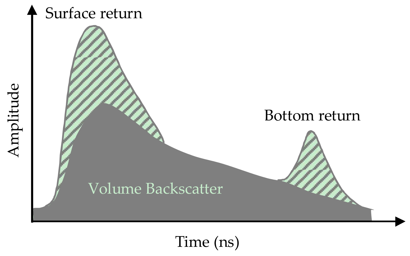
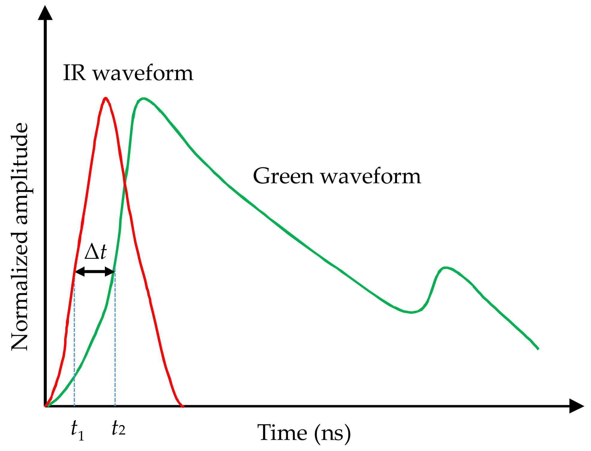
2.1. Traditional Waveform Method
2.2. 3D Point-Cloud Method
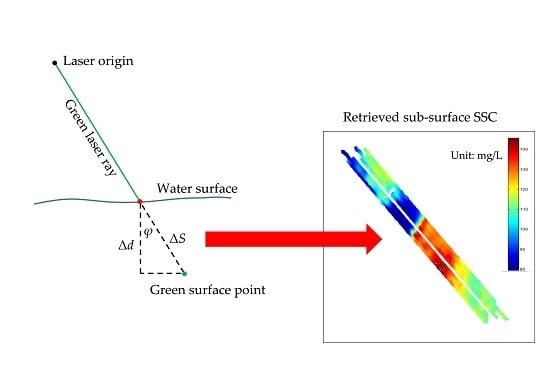
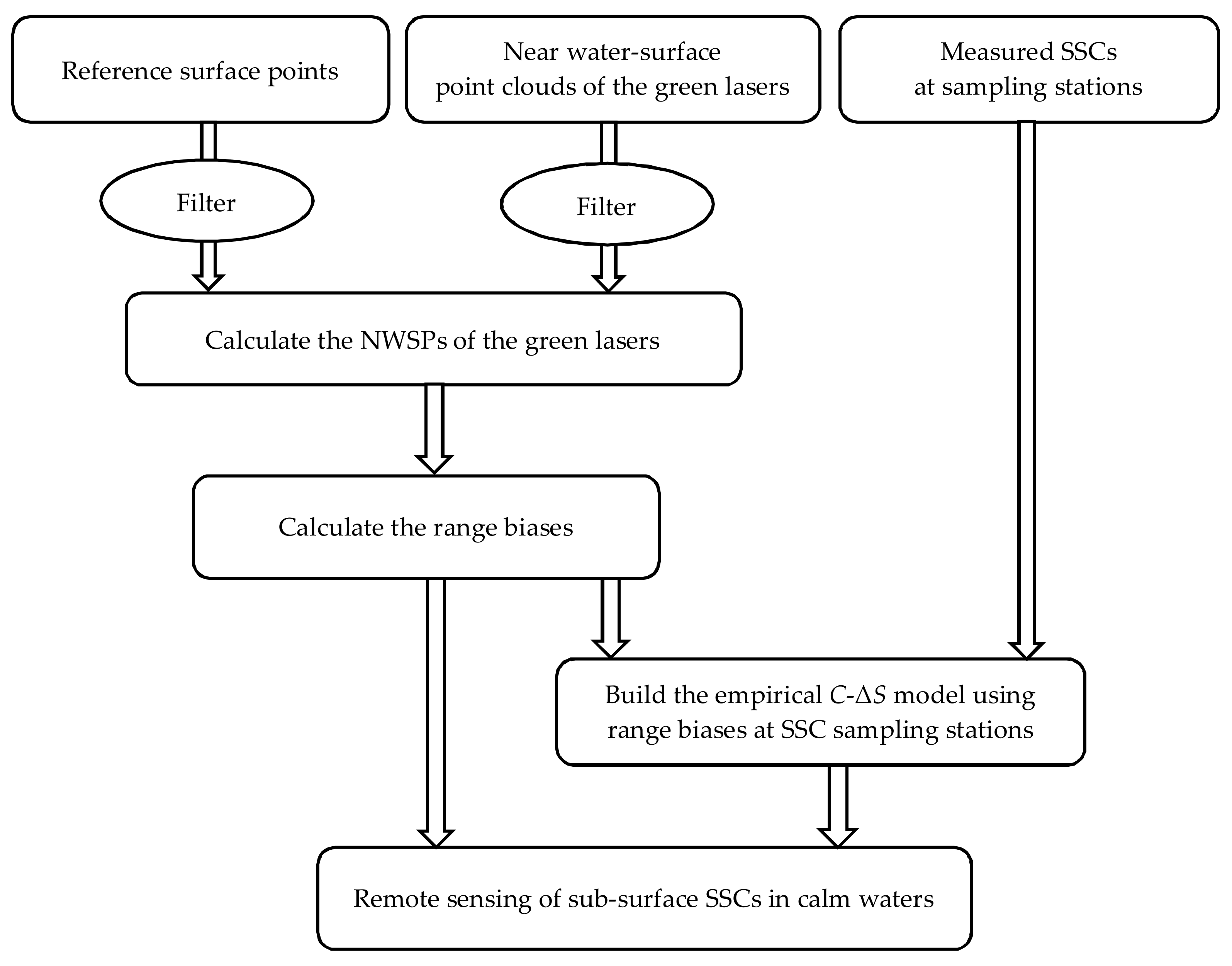
2.3. Steps of Point-Cloud Method
- Step1:
- Extract the green surface points.
- Step2:
- Provide the reference surface points (e.g., IR laser, GPS, or leveling measurements).
- Step3:
- Filter the non-water surface points (e.g., boats, structures, and birds) from the raw 3D point-cloud data.
- Step4:
- Calculate the NWSP Δd of each pulse by using the green surface height and reference surface height.
- Step5:
- Calculate the range bias ΔS by using the corresponding NWSP and the beam-scanning angle.
- Step6:
- Establish the empirical SSC model (C-ΔS) by using the measured SSCs and the range biases at the SSC sampling stations.
- Step7:
- Estimate SSC at each pulse spot by inputting the corresponding NWSP and beam-scanning angle into the constructed C-ΔS model.
3. Experiment and Analysis
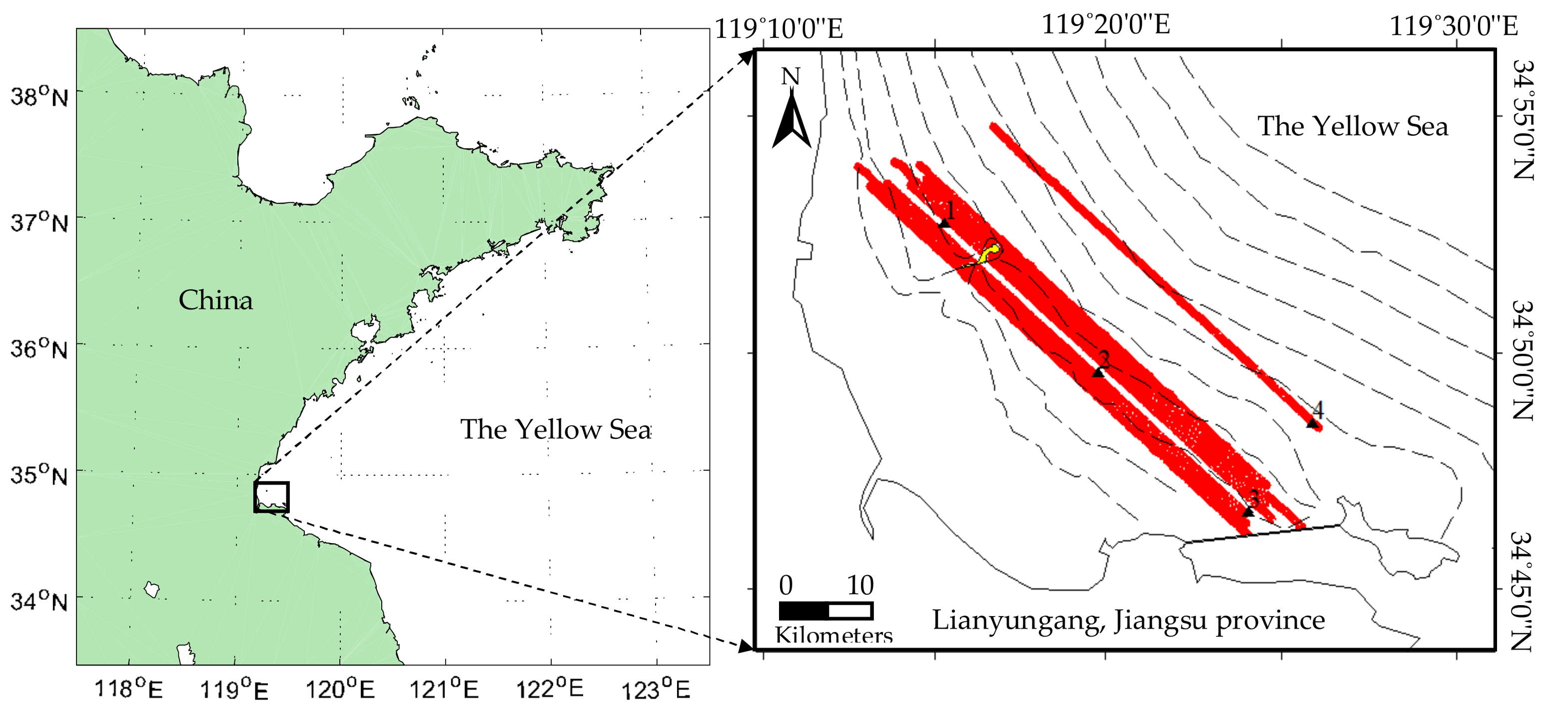
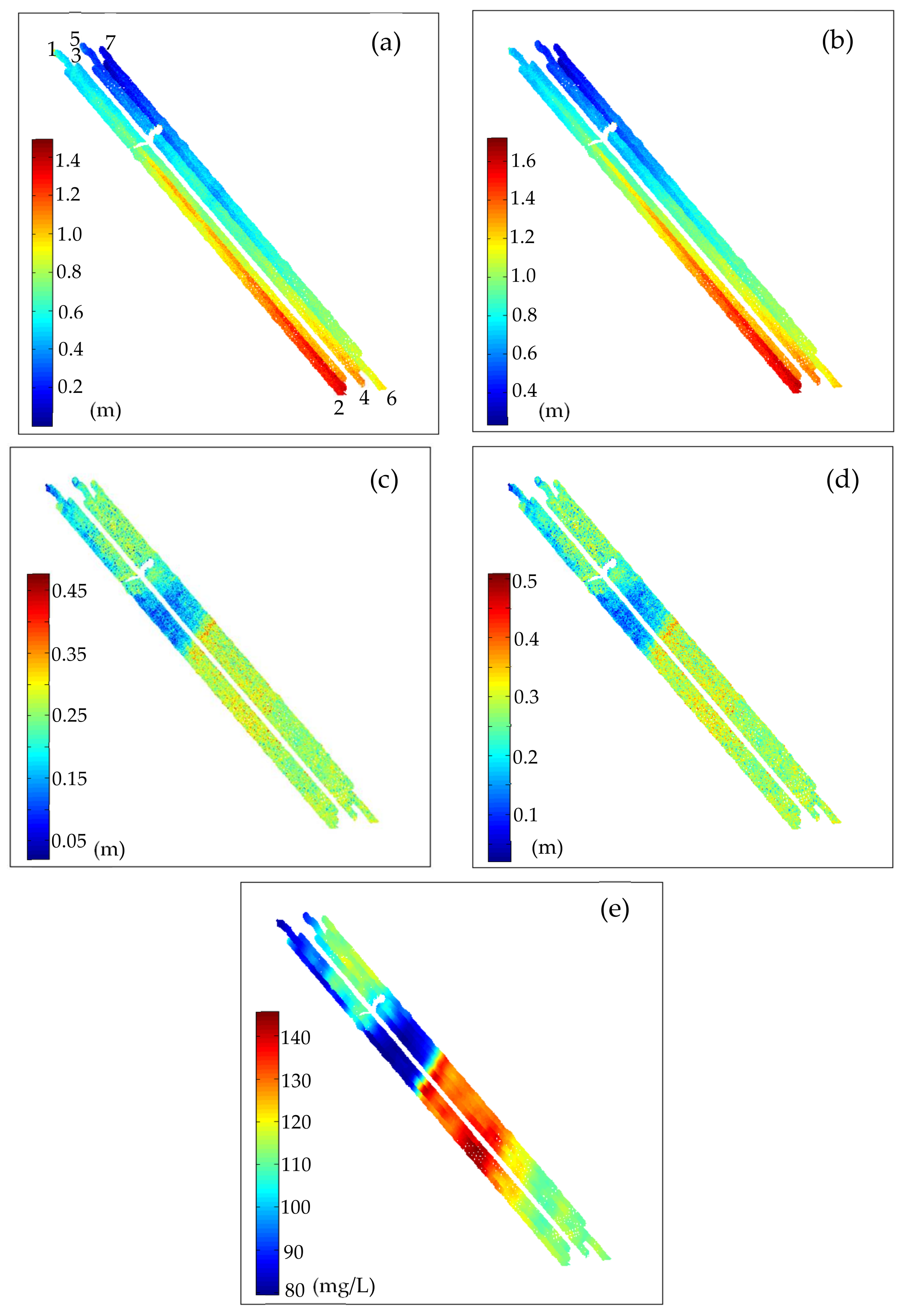
3.1. Data Acquisition
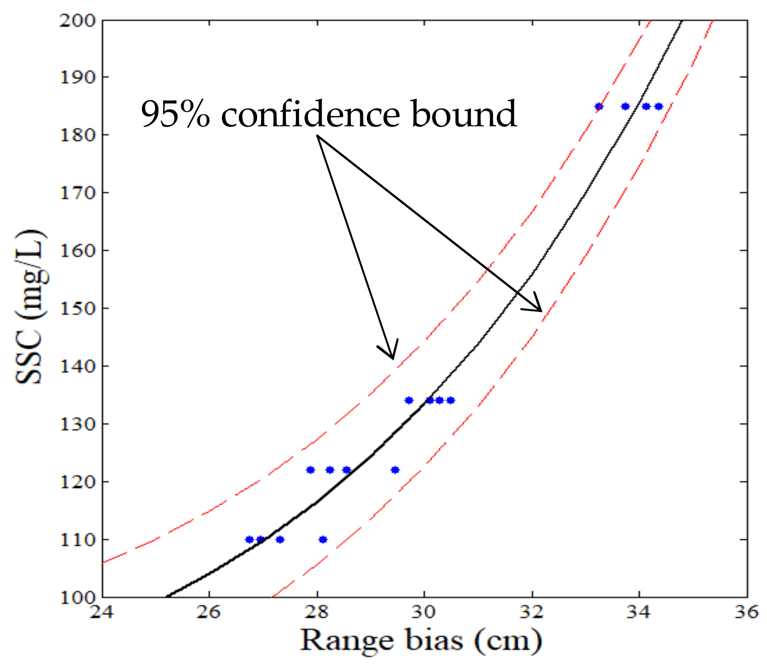
3.2. Establishing the C-ΔS Model
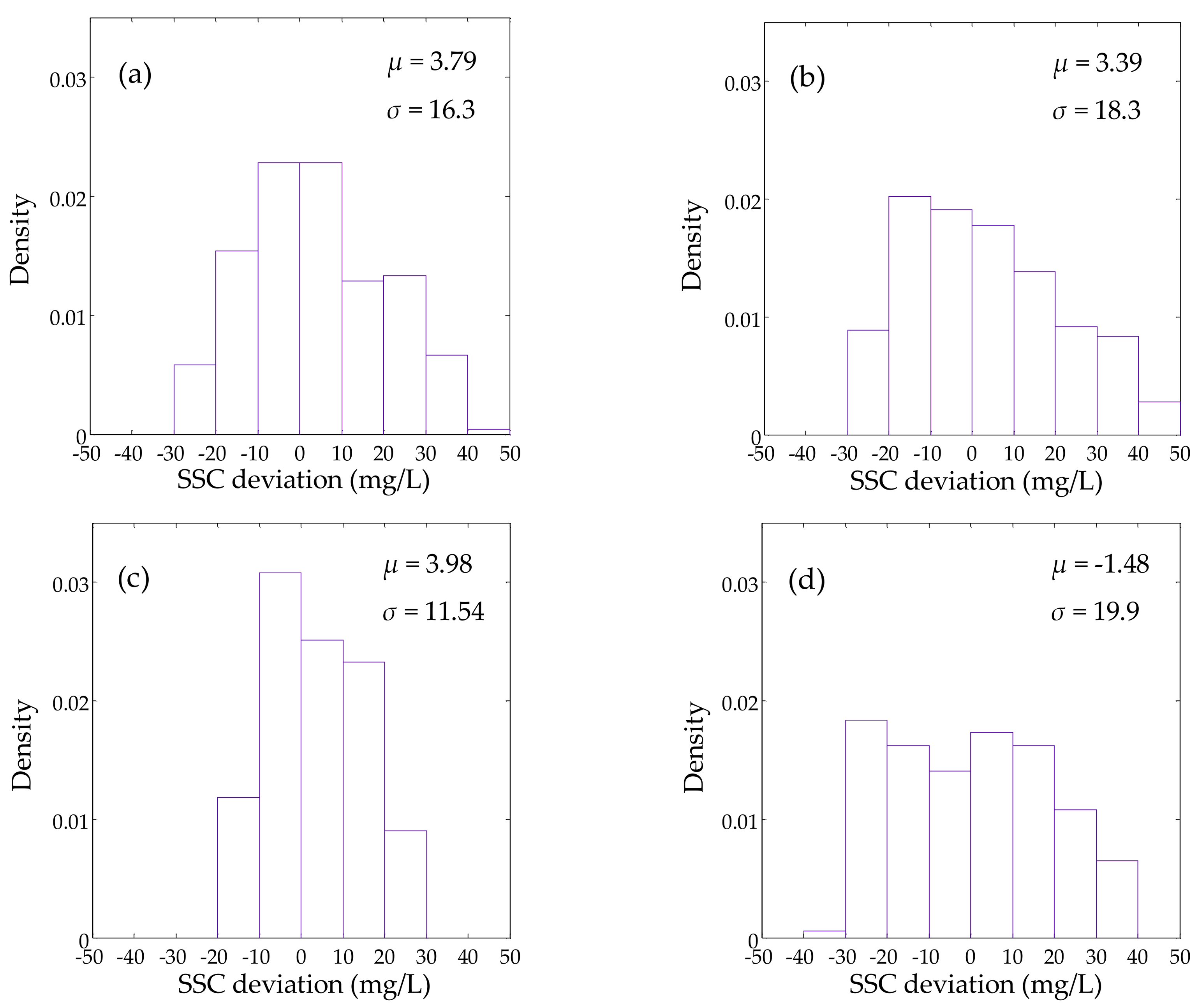
3.3. Precision Analysis
3.4. Remote Sensing of SSCs
4. Discussion
4.1. Reference Surface Height
4.2. SSC Sampling Stations
4.3. Applicability
5. Conclusions and Suggestions
Author Contributions
Acknowledgments
Conflicts of Interest
References
- Qu, L.; Yang, X.; Lei, T. Estimation of suspended sediment concentrations in the Yellow River by network monitoring records and satellite data. In Remote Sensing and Modeling of Ecosystems for Sustainability VIII; International Society for Optics and Photonics: Bellingham, WA, USA, 2011; Volume 8156, p. 81560F. [Google Scholar]
- Epps, S.; Lohrenz, S.; Tuell, G. Development of a suspended particulate matter (SPM) algorithm for the coastal zone mapping and imaging lidar (CZMIL). In Algorithms and Technologies for Multispectral, Hyperspectral, and Ultraspectral Imagery XVI; International Society for Optics and Photonics: Bellingham, WA, USA, 2010; Volume 7695, p. 769514. [Google Scholar]
- Ouillon, S.; Douillet, P.; Andréfouët, S. Coupling satellite data with in situ measurements and numerical modeling to study fine suspended-sediment transport: A study for the lagoon of New Caledonia. Coral Reefs 2004, 23, 109–122. [Google Scholar]
- Churnside, J.H. Review of profiling oceanographic lidar. Opt. Eng. 2013, 53. [Google Scholar] [CrossRef]
- Vasilkov, A.P.; Goldin, Y.A.; Gureev, B.A. Airborne polarized lidar detection of scattering layers in the ocean. Appl. Opt. 2001, 40, 4353–4364. [Google Scholar] [CrossRef] [PubMed]
- Lee, J.H.; Churnside, J.H.; Marchbanks, R.D. Oceanographic lidar profiles compared with estimates from in situ optical measurements. Appl. Opt. 2013, 52, 786–794. [Google Scholar] [CrossRef] [PubMed]
- Allocca, D.M.; London, M.A.; Curran, T.P. Ocean water clarity measurement using shipboard lidar systems. In Ocean Optics: Remote Sensing and Underwater Imaging; International Society for Optics and Photonics: Bellingham, WA, USA, 2002; Volume 4488, pp. 106–115. [Google Scholar]
- Guenther, G.C.; Cunningham, A.G.; Laroque, P.E.; Reid, D.J. Meeting the accuracy challenge in airborne Lidar bathymetry. In Proceedings of the 20th EARSeL Symposium: Workshop on Lidar Remote Sensing of Land and Sea, Dresden, Germany, 16–17 June 2000. [Google Scholar]
- Wong, H.; Antoniou, A. Characterization and decomposition of waveforms for LARSEN 500 airborne system. IEEE Trans. Geosci. Remote Sens. 1991, 29, 912–921. [Google Scholar] [CrossRef]
- Philips, D.M.; Abbot, R.H.; Penny, M.F. Remote sensing of sea water turbidity with an airborne laser system. J. Phys. D Appl. Phys. 1984, 17, 1749–1758. [Google Scholar] [CrossRef]
- Billard, B.; Abbot, R.H.; Penny, M.F. Airborne estimation of sea turbidity parameters from the WRELADS laser airborne depth sounder. Appl. Opt. 1986, 25, 2080–2088. [Google Scholar] [CrossRef] [PubMed]
- Saylam, K.; Brown, R.A.; Hupp, J.R. Assessment of depth and turbidity with airborne Lidar bathymetry and multiband satellite imagery in shallow water bodies of the Alaskan North Slope. Int. J. Appl. Earth Obs. Geoinf. 2017, 58, 191–200. [Google Scholar] [CrossRef]
- Richter, K.; Maas, H.G.; Westfeld, P.; Weiß, R. An Approach to Determining Turbidity and Correcting for Signal Attenuation in Airborne Lidar Bathymetry. PFG J. Photogramm. Remote Sens. Geoinf. Sci. 2017, 85, 31–40. [Google Scholar] [CrossRef]
- Kim, M.; Feygels, V.; Kopilevich, Y.; Park, J.Y. Estimation of inherent optical properties from CZMIL lidar. In Proceedings of the SPIE Asia-Pacific Remote Sensing, Beijing, China, 13–16 October 2014; Volume 9262, p. 92620W. [Google Scholar]
- Zhao, X.; Zhao, J.; Zhang, H.; Zhou, F. Remote Sensing of Suspended Sediment Concentrations Based on the Waveform Decomposition of Airborne LiDAR Bathymetry. Remote Sens. 2018, 10, 247. [Google Scholar] [CrossRef]
- Mandlburger, G.; Pfennigbauer, M.; Pfeifer, N. Analyzing near water surface penetration in laser bathymetry—A case study at the River Pielach. In Proceedings of the ISPRS Annals of the Photogrammetry, Remote Sensing and Spatial Information Sciences, Antalya, Turkey, 11–13 November 2013. [Google Scholar]
- Zhao, J.; Zhao, X.; Zhang, H.; Zhou, F. Shallow Water Measurements Using a Single Green Laser Corrected by Building a Near Water Surface Penetration Model. Remote Sens. 2017, 9, 426. [Google Scholar] [CrossRef]
- Guenther, G.C. Airborne Laser Hydrography: System Design and Performance Factors. Available online: http://shoals.sam.usace.army.mil/downloads/Publications/AirborneLidarHydrography.pdf (accessed on 25 February 2017).
- Saylam, K.; Hupp, J.R.; Averett, A.R. Airborne lidar bathymetry: Assessing quality assurance and quality control methods with Leica Chiroptera examples. Int. J. Remote Sens. 2018, 39, 2518–2542. [Google Scholar] [CrossRef]
- Ritchie, J.C.; Zimba, P.V.; Everitt, J.H. Remote sensing techniques to assess water quality. Photogramm. Eng. Remote Sens. 2003, 69, 695–704. [Google Scholar] [CrossRef]
- MacDonald, C.; Webster, T.; Collins, K.; Crowell, N.; McGuigan, K. Enhanced Subtidal Infrastructure Assessment to Support Inland Finfish Aquaculture. Available online: http://agrg.cogs.nscc.ca/dl/Reports/ 2017/Enhanced%20Subtidal%20Infrastructure%20Assessment%20to%20Support%20Inland%20Finfish%20Aquaculture.pdf (accessed on 20 April 2018).
- Mathur, A.; Ramnath, V.; Feygels, V.; Fuchs, E.; Park, J.Y.; Tuell, G.H. Predicted lidar ranging accuracy for CZMIL. In Algorithms and Technologies for Multispectral, Hyperspectral, and Ultraspectral Imagery XVI; International Society for Optics and Photonics: Bellingham, WA, USA, 2010; Volume 7695, p. 76950Z. [Google Scholar]
- Bouhdaoui, A.; Bailly, J.S.; Baghdadi, N.; Abady, L. Modeling the water bottom geometry effect on peak time shifting in Lidar bathymetric waveforms. IEEE Geosci. Remote Sens. Lett. 2014, 11, 1285–1289. [Google Scholar] [CrossRef]
- Guenther, G.C.; Mesick, H.C. Analysis of airborne laser hydrography waveforms. In Ocean Optics IX; International Society for Optics and Photonics: Bellingham, WA, USA, 1988; Volume 925, pp. 232–242. [Google Scholar]
- Billard, B.; Wilsen, P.J. Sea surface and depth detection in the WRELADS airborne depth sounder. Appl. Opt. 1986, 25, 2059–2066. [Google Scholar] [CrossRef] [PubMed]
- Pan, Z.; Glennie, C.; Hartzell, P.; Fernandez-Diaz, J.C.; Legleiter, C.; Overstreet, B. Performance Assessment of High Resolution Airborne Full Waveform LiDAR for Shallow River Bathymetry. Remote Sens. 2015, 7, 5133–5159. [Google Scholar] [CrossRef]
- Abdallah, H.; Bailly, J.S.; Baghdadi, N.N.; Saint-Geours, N.; Fabre, F. Potential of space-borne LiDAR sensors for global bathymetry in coastal and inland waters. IEEE J. Sel. Top. Appl. Earth Obs. Remote Sens. 2013, 6, 202–216. [Google Scholar] [CrossRef]
- Abady, L.; Bailly, J.S.; Baghdadi, N. Assessment of quadrilateral fitting of the water column contribution in lidar waveforms on bathymetry estimates. IEEE Geosci. Remote Sens. Lett. 2014, 11, 813–817. [Google Scholar] [CrossRef]
- Schwarz, R.; Pfeifer, N.; Pfennigbauer, M.; Ullrich, A. Exponential Decomposition with Implicit Deconvolution of Lidar Backscatter from the Water Column. PFG J. Photogramm. Remote Sens. Geoinf. Sci. 2017, 85, 159–167. [Google Scholar] [CrossRef]
- Wu, J.; Van Aardt, J.A.N.; Asner, G.P. A comparison of signal deconvolution algorithms based on small-footprint lidar waveform simulation. IEEE Trans. Geosci. Remote Sens. 2011, 49, 2402–2414. [Google Scholar] [CrossRef]
- Wang, C.; Li, Q.; Liu, Y.; Wu, G.; Liu, P.; Ding, X. A comparison of waveform processing algorithms for single-wavelength LiDAR bathymetry. ISPRS J. Photogramm. Remote Sens. 2015, 101, 22–35. [Google Scholar] [CrossRef]
- Mandlburger, G. Interaction of Laser Pulses with the Water Surface—Theoretical Aspects and Experimental Results. Allgemeine Vermessungs-Nachrichten 2017, 11–12, 343–352. [Google Scholar]
- Tuell, G.; Barbor, K.; Wozencraft, J. Overview of the coastal zone mapping and imaging lidar (CZMIL): A new multisensor airborne mapping system for the US Army Corps of Engineers. In Algorithms and Technologies for Multispectral, Hyperspectral, and Ultraspectral Imagery XVI; International Society for Optics and Photonics: Bellingham, WA, USA, 2010; Volume 7695, p. 76950R. [Google Scholar]
- Carr, D.A. A study of the Target Detection Capabilities of an Airborne Lidar Bathymetry System. Ph.D. Thesis, Georgia Institute of Technology, Atlanta, GA, USA, 2013. [Google Scholar]
- Quadros, N.D. Unlocking the characteristics of Bathymetric Lidar Sensors. LiDAR Mag. 2013, 3, 62–67. [Google Scholar]
- Habib, A.; Bang, K.I.; Kersting, A.P. Error budget of LiDAR systems and quality control of the derived data. Photogramm. Eng. Remote Sens. 2009, 75, 1093–1108. [Google Scholar] [CrossRef]


| Station Number | Pulse Numbers | Δd (cm) | φ (Degree) | ||||||
|---|---|---|---|---|---|---|---|---|---|
| Max. | Min. | Mean. | SD | Max. | Min. | Mean. | SD | ||
| 1 | 241 | 30.5 | 23.1 | 27.2 | 1.77 | 20.28 | 18.40 | 19.55 | 0.77 |
| 2 | 361 | 31.6 | 25.0 | 28.4 | 1.70 | 20.67 | 18.94 | 19.71 | 0.44 |
| 3 | 220 | 29.0 | 22.4 | 25.8 | 1.71 | 20.58 | 19.33 | 20.22 | 0.25 |
| 4 | 196 | 33.8 | 29.3 | 31.7 | 1.20 | 22.64 | 19.83 | 20.89 | 0.67 |
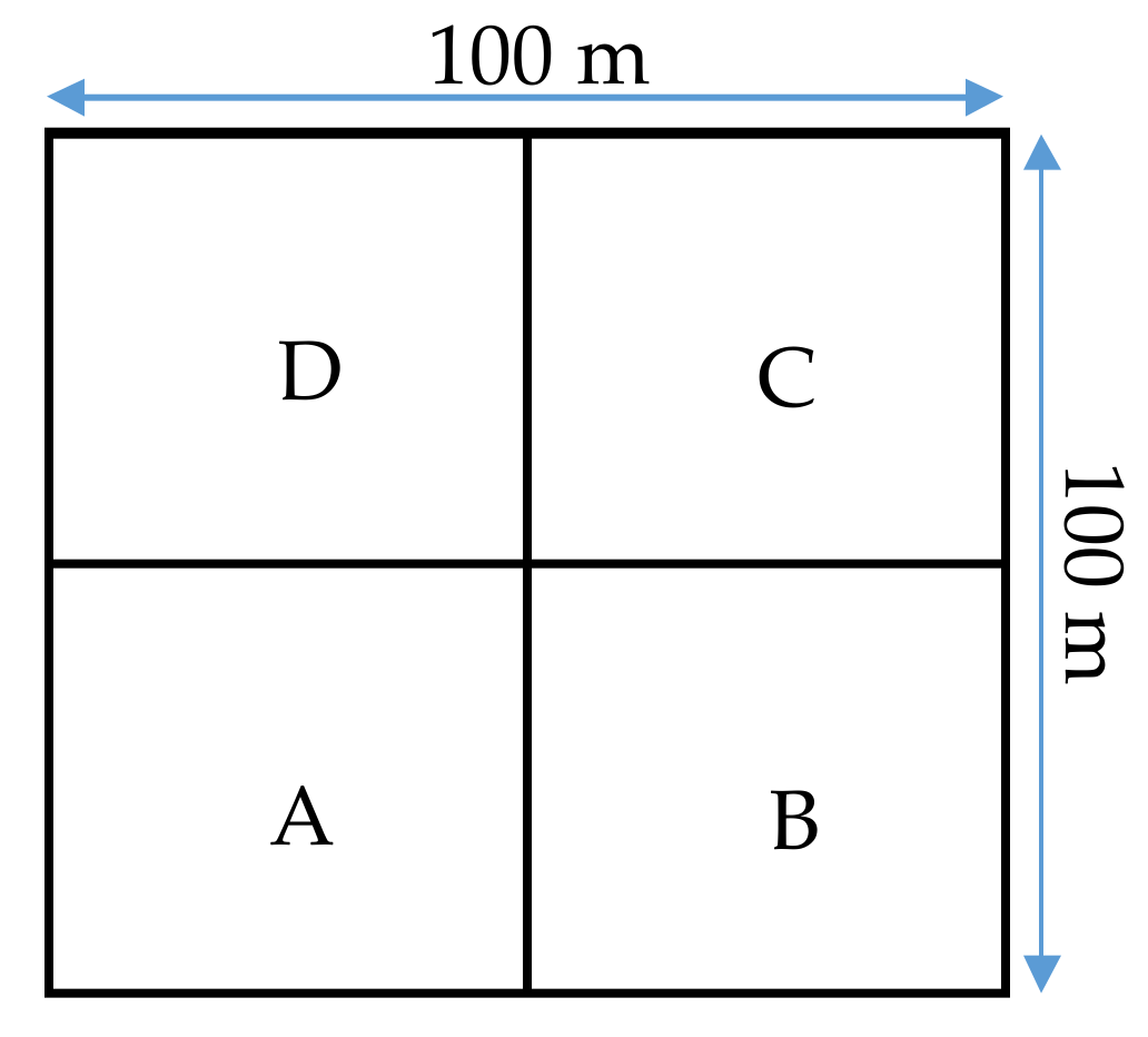
| Station Number | Region | Pulse Numbers | Max. | Min. | Mean | SD |
|---|---|---|---|---|---|---|
| 1 | A | 12 | 31.1 | 25.6 | 27.88 | 1.46 |
| B | 76 | 31.7 | 24.4 | 28.24 | 1.76 | |
| C | 25 | 32.2 | 25.1 | 28.56 | 2.10 | |
| D | 128 | 32.7 | 24.8 | 29.45 | 1.87 | |
| 2 | A | 69 | 33.4 | 26.7 | 29.71 | 1.64 |
| B | 102 | 33.6 | 26.5 | 30.11 | 1.78 | |
| C | 70 | 33.5 | 26.7 | 30.49 | 1.85 | |
| D | 120 | 33.7 | 26.5 | 30.29 | 1.82 | |
| 3 | A | 16 | 30.4 | 24.2 | 26.75 | 1.71 |
| B | 54 | 30.8 | 24.2 | 26.96 | 1.62 | |
| C | 108 | 30.9 | 24.3 | 28.11 | 1.76 | |
| D | 42 | 30.9 | 23.8 | 27.33 | 1.87 | |
| 4 | A | 59 | 37.8 | 30.2 | 34.35 | 1.83 |
| B | 50 | 37.6 | 30.1 | 34.13 | 2.21 | |
| C | 43 | 37.3 | 30.3 | 33.75 | 1.83 | |
| D | 44 | 37.6 | 30.3 | 33.25 | 1.96 |
| Model Coefficients | Value | 95% Confidence Bounds |
|---|---|---|
| a | 8.123 × 10⁻⁷ | (−9.842 × 10⁻⁶, 1.147 × 10⁻⁵) |
| b | 5.303 | (1.691, 8.916) |
| c | 78.06 | (35.29, 120.8) |
© 2018 by the authors. Licensee MDPI, Basel, Switzerland. This article is an open access article distributed under the terms and conditions of the Creative Commons Attribution (CC BY) license (http://creativecommons.org/licenses/by/4.0/).
Share and Cite
Zhao, X.; Zhao, J.; Zhang, H.; Zhou, F. Remote Sensing of Sub-Surface Suspended Sediment Concentration by Using the Range Bias of Green Surface Point of Airborne LiDAR Bathymetry. Remote Sens. 2018, 10, 681. https://0-doi-org.brum.beds.ac.uk/10.3390/rs10050681
Zhao X, Zhao J, Zhang H, Zhou F. Remote Sensing of Sub-Surface Suspended Sediment Concentration by Using the Range Bias of Green Surface Point of Airborne LiDAR Bathymetry. Remote Sensing. 2018; 10(5):681. https://0-doi-org.brum.beds.ac.uk/10.3390/rs10050681
Chicago/Turabian StyleZhao, Xinglei, Jianhu Zhao, Hongmei Zhang, and Fengnian Zhou. 2018. "Remote Sensing of Sub-Surface Suspended Sediment Concentration by Using the Range Bias of Green Surface Point of Airborne LiDAR Bathymetry" Remote Sensing 10, no. 5: 681. https://0-doi-org.brum.beds.ac.uk/10.3390/rs10050681