Using a Virtual Lidar Approach to Assess the Accuracy of the Volumetric Reconstruction of a Wind Turbine Wake

Abstract

Scanning Doppler lidars are the best tools for acquiring 3D velocity fields of full scale wind turbine wakes, whether the objective is a better understanding of some features of the wake or the validation of wake models. Since these lidars are based on the Doppler effect, a single scanning lidar normally relies on certain assumptions when estimating some components of the wind velocity vector. Furthermore, in order to reconstruct volumetric information, one needs to aggregate data, perform statistics on it and, most likely, interpolate to a convenient coordinate system, all of which introduce uncertainty in the measurements. This study simulates the performance of a virtual lidar performing stacked step-and-stare plan position indicator (PPI) scans on large-eddy simulation (LES) data, reconstructs the wake in terms of the average and the standard deviation of the longitudinal velocity component, and quantifies the errors. The variables included in the study are as follows: the location of the lidar (ground-based and nacelle-mounted), different atmospheric conditions, and varying scan speeds, which in turn determine the angular resolution of the measurements. Testing different angular resolutions allows one to find an optimum that balances the different error sources and minimizes the total error. An optimum angular resolution of 3${}^{\circ }$ has been found to provide the best results. The errors found when reconstructing the average velocity are low (less than 2% of the freestream velocity at hub height), which indicates the possibility of high quality field measurements with an optimal angular resolution. The errors made when calculating the standard deviation are similar in magnitude, although higher in relative terms than for the mean, thus leading to a poorer quality estimation of the standard deviation. This holds true for the different inflow cases studied and for both ground-based and nacelle-mounted lidars.

1. Introduction

Wind power growth worldwide is a result of an ever increasing demand for renewable energy. With upper limits of rated power for single turbines reaching the order of 10 MW, the common solution to keep increasing the generated power is to install a larger number of wind turbines. Due to space limitations, in most cases, wind turbines are clustered together in wind farms and effectively this means a higher number of turbines in each wind farm. In large wind farms, most of the wind turbines are affected by the wake flow of others, resulting in a reduction of incoming wind speed and an increase of turbulence [1]. Therefore, a careful evaluation of wind resources is needed for an accurate estimation of not only produced power from a future wind farm [2,3], but also the power losses and increased fatigue loads associated with the wind turbine wakes [4]. Accurate wake models are needed to that end, and the location of each of the wind turbines inside the farm needs to be optimized in order to minimize the losses [5,6].

There are a number of strategies to model the wake of a wind turbine: numerical models [7] discretize the Navier–Stokes (N.S.) equations, either in the physical space or the Fourier space, and solve them with the help of various turbulence models; analytical models [8] use certain assumptions (e.g., the shape of the wind velocity deficit in the wake) and combine them with the N.S. equations either in 1D or 3D; lastly, empirical models can be based on either measurements alone or a mixture between important simplifications of the Navier–Stokes equations and empirical parameters [9]. All of them must, inevitably, be contrasted with measurements of wind turbine wakes in order to estimate their accuracy and, if applicable, be validated under certain conditions.

The interaction between the atmospheric boundary layer (ABL) and a full scale wind turbine is a three-dimensional, dynamic flow phenomenon that extends from approximately two diameters in front of the rotor to several hundred meters, possibly a few kilometers, downwind [1]. The ideal measurement set for a characterization of a single wind turbine wake would include the three components of the wind velocity vector, at all times and at all positions in space within the region of influence. Unfortunately, no measurement technique is able to provide such data. Different instruments provide different sets of measurements, with varying levels of suitability for the characterization of a wind turbine wake.

The standard instrument for turbulence measurements in the atmosphere, the sonic anemometer, is not well suited for the measurement of turbine wake flows. Sonic anemometers only offer point-wise information and it is not practical to cover an extensive volume by mounting them on meteorological masts. Alternatives to the sonic anemometer and the meteorological mast are, in some cases, unmanned aerial vehicle platforms, since they are able to fly and measure in any point in space [10,11,12,13,14]. Nevertheless, they have important limitations: most of them are s till mostly in prototype phase, they are not suitable for long-term statistics, and covering a volume with point-wise measurements would imply thousands of hours of flight.

As an alternative, remote sensing techniques are increasingly popular in atmospheric flows because of their ability to measure where other sensors cannot. Among these, Doppler light detection and ranging (lidar) is the preferred remote sensing technique for atmospheric turbulence measurements due to its accuracy and relatively high spatial resolution and long range. As of today, it is the most suitable measurement technique to study the different characteristics of wind turbine wakes [15,16,17,18,19,20,21,22,23].

One limitation of the lidar technique arises from the fact that it is based on the Doppler effect and uses backscattered light from aerosol. Therefore, it can only measure the velocity component parallel to the laser beam (radial velocity). A scanning Doppler lidar can orient its laser beam in any direction; this implies that, unless the laser beam is completely vertical or aligned with the direction of the flow or transversal to it, the measured velocity is normally a mixture of the three components of the wind velocity vector. As a consequence, most lidar measurements rely on some assumptions when calculating the relevant variables such as horizontal wind speed, vertical wind speed, or the different turbulence quantities [24,25,26]. Multiple-lidar techniques exist and can overcome this limitation [27,28,29] although they multiply the cost, are more cumbersome to use, and require a significantly higher degree of expertise to be properly operated. The use of a single lidar and the necessary assumptions is a source of uncertainty that needs to be estimated.

Another limitation of the lidar technique is the speed of the measurements. A scanning pulsed lidar emits several thousand laser pulses in a particular direction or line-of-sight (LoS), evaluates the backscattered signal, calculates the Doppler shift at different distances from the lidar, and then proceeds to the next laser beam orientation. Since a wind turbine wake is inherently dynamic, in order to cover a volume with lidar measurements, a scanning strategy is needed in order to balance angular resolution and number of measurements at each orientation. This translates into finding a compromise between a spatial interpolation error and a statistical uncertainty. These two need to be estimated as well.

As discussed above, no technique is able to provide the velocity field in order to estimate the errors and uncertainties associated with a volumetric lidar scan of a wind turbine wake. Therefore, a good strategy is to use a virtual lidar technique to perform a virtual experiment. Specifically, a turbulence-resolving large-eddy simulation (LES) is performed and then the characteristics and scanning pattern of a virtual instrument can be programmed to extract information or virtual measurements from LES simulated velocity field. These virtual measurements can be post-processed with the same algorithms used to treat real measurements in order to reconstruct the desired flow feature (in this case, the far wake of the wind turbine) and then it can be compared to the original velocity field from the LES simulation. A virtual lidar technique allows the estimation of the different sources of uncertainties or errors separately. In this manuscript, the sources of error studied are three: the assumptions used to convert the radial velocity to longitudinal velocity, the statistical error, and the interpolation error. Finally, testing different scanning patterns allows one to find an optimum that minimizes the errors. The error magnitude, in turn, will determine the quality of future real (time and resource-consuming) field experiments.

Most of the literature regarding virtual lidar studies is very recent. Stawiarski et al. [30] created a virtual lidar measurement simulator based on LES results in which lidar characteristics such as range gate length, pulse length, total range, and measurement frequency are adjustable. In their simulator, they include the effect of the convolution of the laser pulse as a cylindrical volume centered around the range gate center, and they use a weighted averaging function over the LES data points inside that volume. They discuss extensively the different kinds of errors connected with single- and double-lidar measurements and provide the methodology to study the sources of errors and the optimization of dual-Doppler scan patterns. Stawiarski et al. [31] further performed virtual planar dual-lidar experiments to study the reconstruction and the detection of planar turbulent structures.

Lundquist et al. [32] studied the uncertainty of the Doppler beam swinging (DBS) technique, used by many commercial profiling lidars, when calculating horizontal and vertical velocities while violating the assumption of horizontally homogeneous flow that the technique requires. The calculation of the vertical profiles of horizontal velocity is done using virtual measurements obtained from LES simulations of a wind turbine wake. Similarly, Mirocha et al. [33] have simulated the effect of the inhomogeneity on profiling lidar measurements using a virtual lidar technique approach under different atmospheric stability conditions.

Van Dooren et al. [34] used virtual lidar experiments to explore the possibilities and uncertainty of wind turbine wake reconstruction with ground-based dual-lidar plan position indicator (PPI) scans. For that, they obtained non-synchronous dual-Doppler lidar measurements from LES simulations, and they improved the accuracy of the reconstructed wind field by including a correction based on the mass continuity equation.

Meyer Forsting et al. [35] developed a novel validation methodology for computational fluid dynamics (CFD) models over the wind turbine induction zone using measurements from three synchronous lidars. The validation procedure relied on making the CFD simulation results comparable with the triple lidar data. To that end, they discretized in space the probability density function of the measured free-stream wind speed. Then they reproduced those distributions numerically by weighting the steady-state Reynolds averaged Navier–Stokes simulations. As a last step, the spatial and temporal uncertainty of the triple lidar measurements were quantified and propagated through the data processing.

Lastly, and although the virtual lidar technique is not used, it is worth mentioning that van Dooren et al. [36] studied the uncertainty of synchronous short-range continuous dual-lidar measurements for the measurement of scaled wind turbine wakes placed inside a wind tunnel. They were able to compare the estimated uncertainty of some of their configurations by comparing the lidar measurements to those taken by a triple hot-wire probe.

In this study, a virtual lidar technique based on LES simulations, similar to what has been used in some of the above-mentioned references, is used to calculate different error sources for a single pulsed lidar performing volumetric scans of a full scale wind turbine wake under different atmospheric conditions and for two different lidar locations: nacelle-mounted and ground-based. The technique allows one to optimize the scanning of the wake and evaluate the quality of the measurement strategy and the assumptions used for the treatment of the data.

There are a number of practical advantages to using nacelle-mounted lidars over ground-based ones. Arguably, the most important one is the fact that a lidar fixed to the structure of the nacelle of a wind turbine always maintains the same angular orientation with respect to the rotor. This means that it does not need any reorientation with a changing wind direction and it never gets blocked by the tower of the turbine. Nevertheless, practical considerations of this kind are beyond the scope of this study.

2. Methodology

A virtual lidar approach is based on the idea of performing virtual experiments on a flow field in which the three components of the wind velocity vector $\mathbf{v}(x,y,z,t)$ are calculated at each point in space and at each point in time. A convenient way of creating such a flow field is through LES simulations. The results of these simulations can be interpreted as a virtual reality from which lidar virtual measurements can be extracted, knowing the characteristics of a particular lidar (spatial resolution, repetition rate, range, etc.), its scanning pattern, and that it measures only the projection of the wind velocity vector onto the laser beam direction or LoS. The lidar virtual measurements obtained can then be processed by the same algorithm used to treat real lidar measurements in order to reconstruct a particular flow feature. Examples include vertical wind profiles in the ABL, 2D horizontal velocity fields of atmospheric surface layer flow, and 3D velocity fields of wind turbine wakes. The reconstructed flow features can be compared to those obtained from the complete three-dimensional, unsteady LES flow fields as a way to estimate the errors introduced by the assumptions used in the algorithm, by the spatial interpolation, and by the limited number of samples in time (statistical error). This also allows for the optimization of scanning patterns in order to minimize the uncertainty for a particular type of experiment.

Next, details are provided about the LES simulations used in this study, the characteristics of the virtual lidar and its scanning strategy, the algorithm for the reconstruction of the 3D flow field, and the optimization process.

2.1. LES Simulations

The virtual measurements are extracted from the results of LES simulations of the interaction of a single turbine with atmospheric boundary layer flow on flat terrain. The WiRE-LES code, described in detail in [37,38,39], was used for the simulations.

2.1.1. Turbulence Model, Boundary Conditions, and Numerical Methods

LES solves the spatially filtered Navier–Stokes equations and, therefore, solves explicitly all the scales of turbulence greater than the filter scale (same as the grid scale for implicit filters), while the subgrid-scale stresses (SGSs) are parameterized using a subgrid-scale model. In the case of the WiRE-LES code, the spatial derivatives are discretized using a pseudospectral representation for the horizontal directions (hence, periodic lateral boundary conditions) and second-order finite differences for the vertical direction, with a wall modeling based on the log law for the bottom boundary. The top boundary condition is a fixed stress-free lid. The code is fully dealiased using the 3/2 rule and the temporal advancement of the simulation uses a second-order accurate Adams–Bashforth scheme. The SGS turbulence model is the Lagrangian scale-dependent dynamic model detailed in [40,41].

2.1.2. Domain Size and Resolution

The domain size is 3200 m in the longitudinal direction (x), 800 m in the transversal direction (y), and 500 m in the vertical direction (z). The domain is divided uniformly into 160 × 60 × 64 grid points, respectively, which yields a spatial resolution of 20 m in x, 13.3 m in y, and 7.8 m in z.

Since in the horizontal direction, there are periodic boundary conditions, a buffer zone upstream of the wind turbine is required in order to create an undisturbed incoming flow. The inflow condition is obtained via a separate precursor simulation.

2.1.3. Inflow

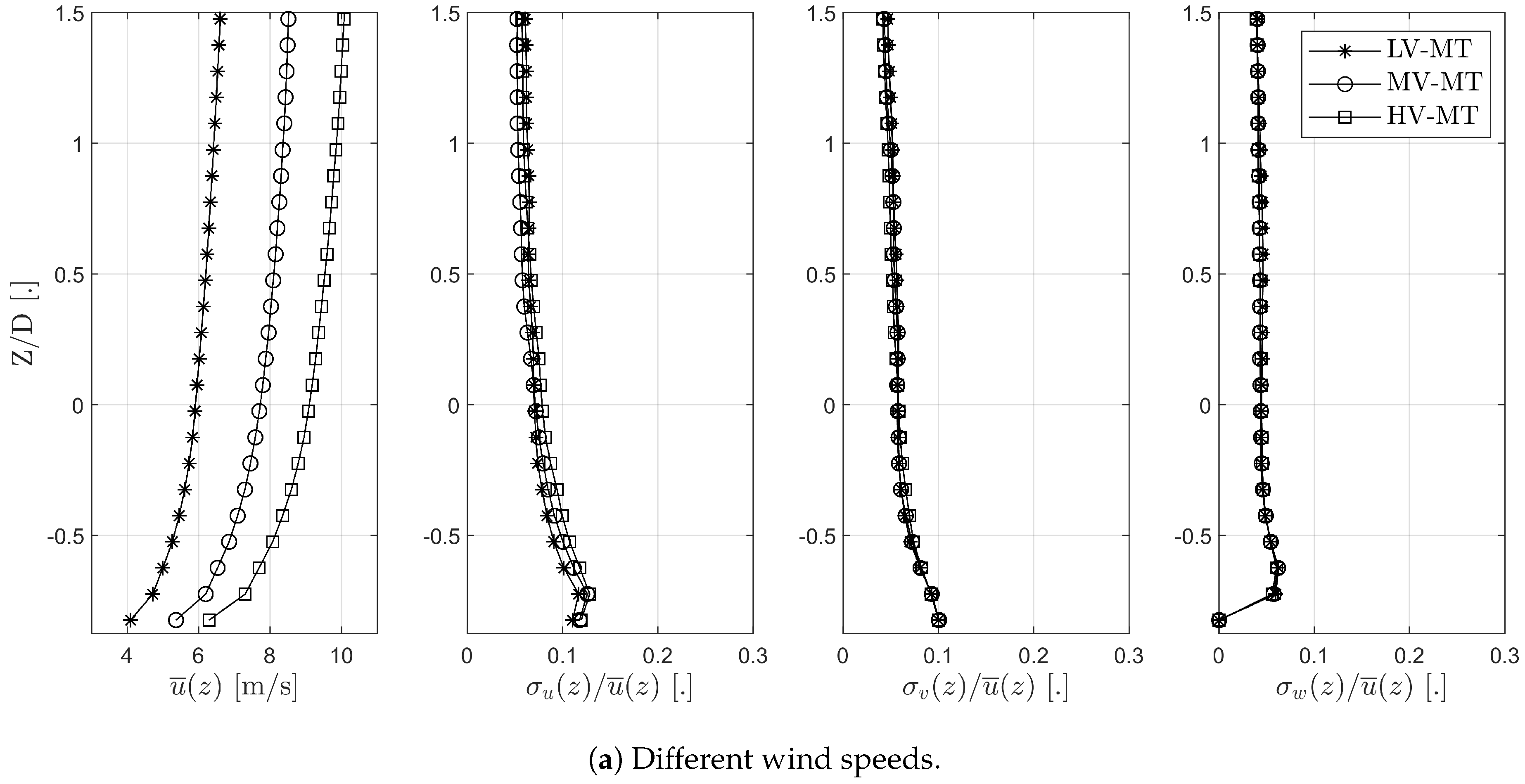
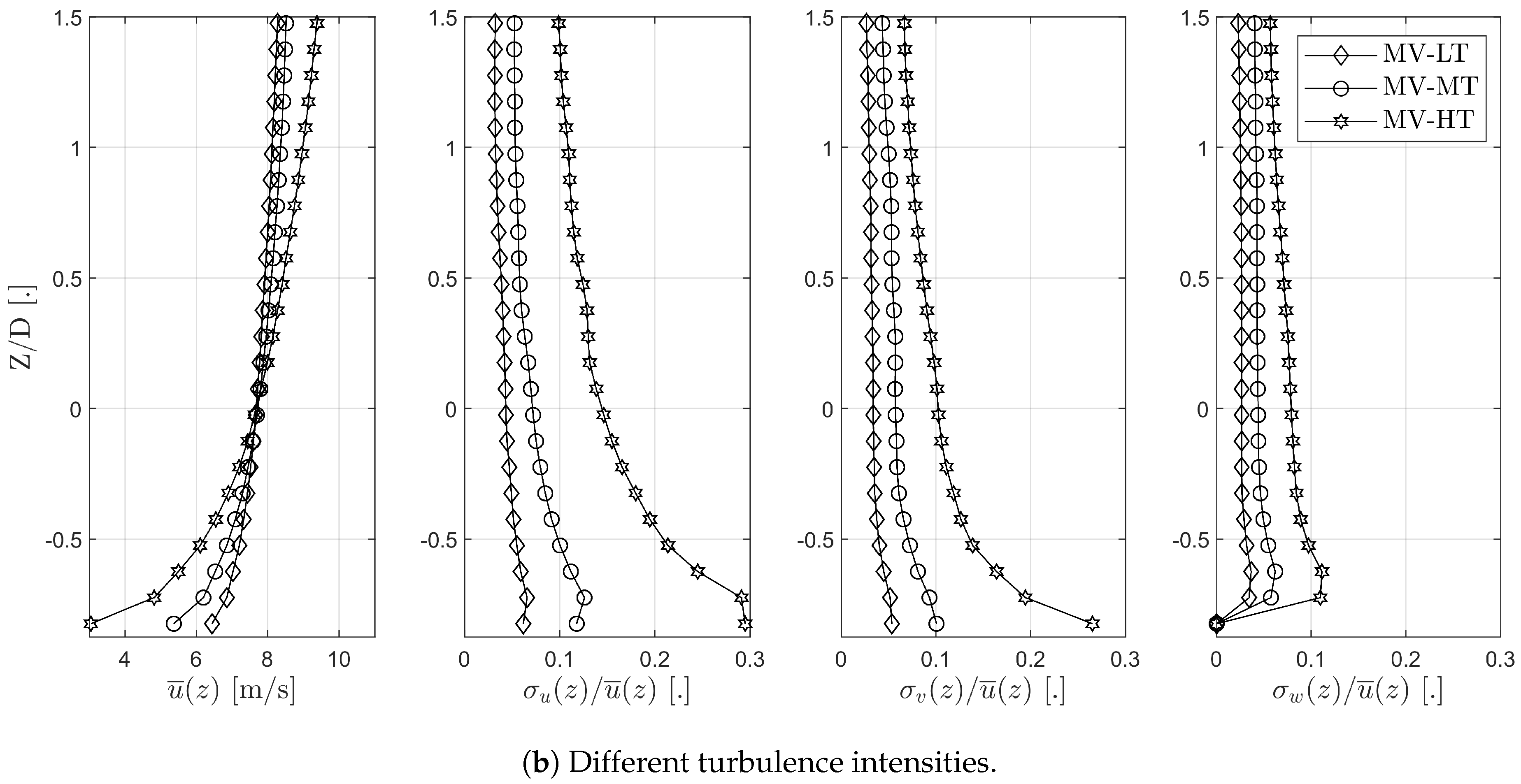
The boundary-layer flow in the simulations is driven by a constant streamwise pressure gradient over flat homogeneous surfaces and is neutrally stratified. Five inflow conditions are used in order to study the influence of different wind speeds and different turbulence intensities. The different turbulence intensities are recreated by using different surface roughness lengths. They are chosen to cover a very wide range between the lowest value corresponding to water or sand (0.0002 m) to grass-covered land (0.005 m) and finally the highest roughness corresponding to suburban or forestal land (0.5 m) [42]. Different wind speeds at hub height are achieved by modifying the forcing longitudinal pressure gradient $dP/dx$. The wind speeds selected (6, 7.5, and 9 m/s) cover the range in which the turbine operates at maximum efficiency $C_P\simeq 0.42$ and maximum thrust $C_T\simeq 0.80$.

The nomenclature of the different inflow cases is (X)V-(X)T, where V denotes wind velocity, T denotes turbulence intensity, and finally (X) can be L-low, M-medium, or H-high (e.g., MV-HT indicates medium wind speed and high turbulence intensity). Figure 1 shows the different inflow conditions for the five simulations.

The coordinate system used in this manuscript has its origin at the center of the rotor, and the longitudinal, transversal, and vertical directions are represented by X, Y, and Z, respectively. Distances appear normalized by the rotor diameter D, which is 80 m, as described in the section below.

2.1.4. Turbine Modeling

The simulation of the aerodynamic forces of the wind turbine and their interaction with the ABL flow is performed through an actuator disk model that includes rotation as described in [37,38], where the lift and drag forces of the wind turbine blades are calculated using Blade-Element Momentum theory (BEM) and distributed in a Gaussian manner by convolving the local load and a regularization kernel [43] and integrated over the spatial and temporal resolution of the simulation.

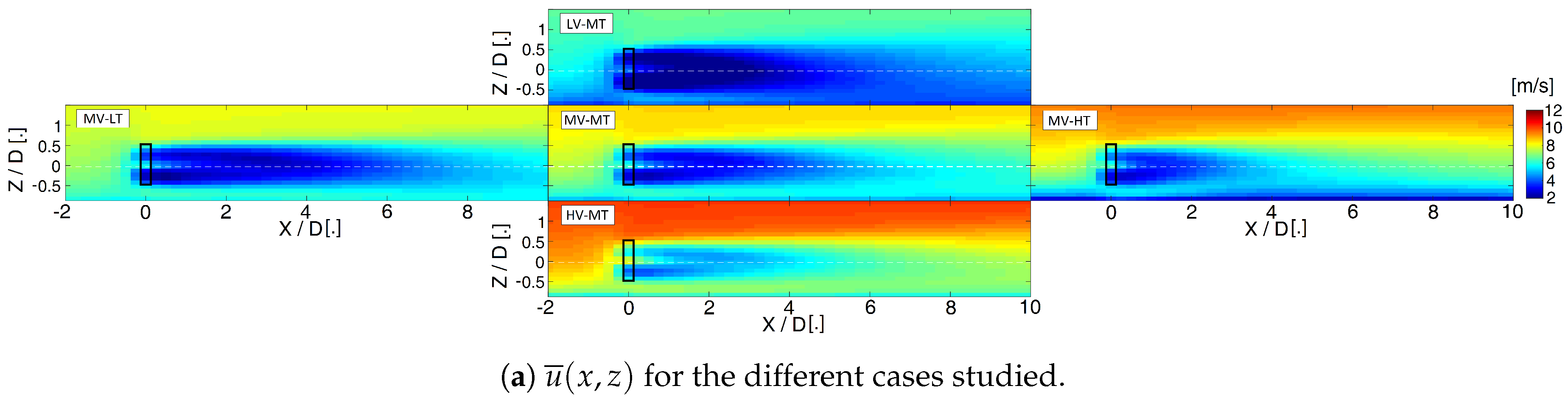
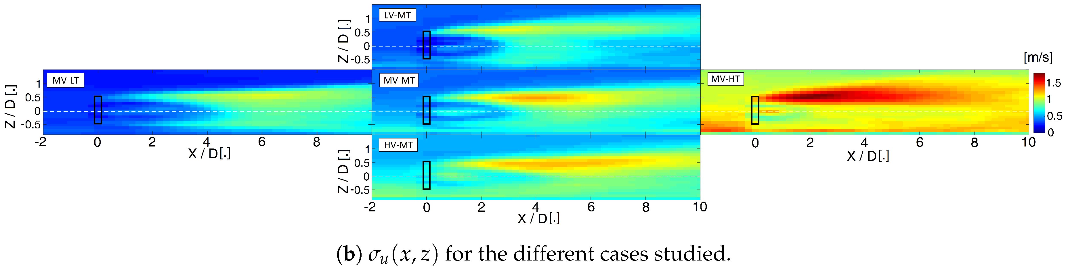
The wind turbine simulated is a V80-2.0 MW Vestas wind turbine with a hub height of 70 m and a rotor diameter of 80 m. All the details of the modeling of the wind turbine can be found in [39]. The results of the simulations are shown in Figure 2 as vertical planes at Y = 0 of the temporal average of the longitudinal component of the wind speed $\overline{u}$ and its standard deviation ${\sigma }_u$.

The simulations were first run for a period of time long enough to achieve stationary flow conditions, and a period of 30 min was then used to sample the simulation results at a resolution of 2 Hz.

2.2. Lidar Virtual Measurements

The lidar simulated in this study is a Halo-Photonics Streamline lidar. It is a pulsed Doppler scanning lidar, which means that it provides measurements of the radial velocity $Vr$ (the projection of the wind velocity into the LoS) at regular distance intervals along the laser beam direction. In this case, the Streamline lidar is able to provide a spatial resolution of 18 m along its LoS, at an acquisition frequency of 2 Hz. The range has been set to infinite since, on our own experience, it exceeds 1.5 km under most atmospheric conditions.

The virtual radial velocity measurements taken by the lidar are then calculated as

$$Vr\left(t\right)=u(x,y,z,t)cos\left(\theta \right(t\left)\right)cos\left(\phi \right(t\left)\right)+v(x,y,z,t)cos\left(\theta \right(t\left)\right)sin\left(\phi \right(t\left)\right)+w(x,y,z,t)sin\left(\theta \right(t\left)\right)$$

(1)

where u, v, and w are the components of the wind velocity vector field from the LES simulations, and are defined in space $(x,y,z)$ and time $\left(t\right)$, $\phi$ is the azimuth angle (angle between the laser beam and the the vertical plane at Y = 0 of the wake), and $\theta$ is the elevation angle (angle between the laser beam and a horizontal plane) that define the orientation of the laser beam in time.

The formally correct calculation of the virtual radial velocity for each laser gate of 18 m would be a convolution of the envelope of the laser pulse on the simulated and projected velocity field [44]. In this study, the convolution is not calculated and the result is instead a point-wise calculation in the linearly interpolated projected field every 18 m. The reason for this is that the resolution of the LES simulation (20 m in the longitudinal direction) is almost the same as the lidar one. This means that the lidar convolution is similar to the spatial filtering already performed by the LES.

The effect of the spatial convolution of high-resolution (20 m) lidar measurements in the attenuation of the longitudinal turbulence intensity has been studied by comparing lidar measurements to sonic anemometry [27]. These experiments, under arguably less favorable conditions than the virtual setup presented here, have shown that the attenuation is in the order of a few tenths of a percentage point, since most of the energy-containing scales are resolved at that resolution. These results may not be extended to lower resolution measurements. No significant effect is expected when reconstructing average velocity fields.

It must be noted that in this study the accuracy of the lidar (instrument error) is neglected. The virtual measurement of the radial velocity (Equation (1)) could include a random error that varies for each instrument and that it depends on the signal-to-noise ratio (SNR) of each measurement. This, in turn, depends on the quality of the different optical parts of the instrument, the power of the laser pulse, the aerosol content, the humidity, and other parameters related to the processing of the Doppler signal such as the length of the laser gate or the number of pulses averaged. It has been shown that a similar pulsed Doppler lidar to the one discussed in this study can achieve, with favorable SNR, accuracies in the order of $\pm 0.1$ m/s or lower [45]. In theory, the effect of simulating this error for any particular instrument will have the effect of slightly increasing the statistical error (in a random manner, therefore no bias introduced) and slightly increasing the standard deviation measurements (therefore, inducing a small bias). Nevertheless, the instrument error of an accurate lidar should be significantly smaller than the turbulent velocity fluctuations found in the wake of a wind turbine and can, in most of the cases, be neglected.

Finally, if a continuous scanning strategy is chosen, the radial velocity calculation has to include the convolution along the arc that the lidar gate covers between two consecutive measurements. This effect can be particularly important when calculating the standard deviation of the radial velocity for locations far downstream and for low angular resolutions of the measurements. On the other hand, a step-and-stare scan avoids this convolution and arguably provides a better estimation of the turbulent fluctuations. This is why only step-and-stare scans are considered in this study.

2.3. Scanning Strategy and Reconstruction of 3D Fields

Depending on the position of the lidar, the ranges of the azimuth and elevation angles are calculated in order to cover the whole volume of interest and are shown in

Table 1. Ranges of the azimuth and elevation angles needed to cover the whole volume of interest for both lidar locations.

	Nacelle-Mounted	Ground-Based
Azimuth angle range	$-{16.7}^{\circ }$ to $+{16.7}^{\circ }$	$-{16.7}^{\circ }$ to $+{16.7}^{\circ }$
Elevation angle range	$-{16.7}^{\circ }$ to $+{16.7}^{\circ }$	$+{1.3}^{\circ }$ to $+{34.0}^{\circ }$

. A pulsed scanning lidar can only measure along a particular direction each time, which implies that there will have to be a compromise between the number of measurements at each point and the angular resolution. Due to the wake being quasi-axial symmetric, the angular resolution is kept the same for the elevation and the azimuth angles. Once a particular angular resolution is set, the virtual lidar scans the volume of interest in consecutive step-and-stare swipes at constant elevation angles (equivalent to PPI scans) at a frequency of 2 Hz between measurements until the end of the 30 min period of each simulation.

The reconstruction of the longitudinal velocity field at the volume of interest is similar to the procedure described in [16,18] and starts by calculating the average of the radial velocity measurements $\overline{Vr}(\phi ,\theta ,r)$ for each laser beam orientation determined by the angles $\phi$ and $\theta$ and distance r, creating a regular spherical grid with the origin at the lidar location. It continues with the assumption of a negligible effect of the average transversal and vertical components of the velocity into the projection on the laser beam direction: $\overline{v}(x,y,z)cos\left(\theta \right)sin\left(\phi \right)=0$; $\overline{w}(x,y,z)sin\left(\theta \right)=0$. This allows one to reconstruct the longitudinal component of the velocity from the radial velocity measurement simply by

$$\overline{u}(\phi ,\theta ,r)=\frac{\overline{Vr}(\phi ,\theta ,r)}{cos\left(\theta \right)cos\left(\phi \right)}.$$

(2)

The error of this assumption is simply calculated as

$$\epsilon =\overline{v}(x,y,z)cos\left(\theta \right)sin\left(\phi \right)+\overline{w}(x,y,z)sin\left(\theta \right).$$

(3)

The reconstruction of the standard deviation field of the longitudinal velocity component uses a different assumption (stronger than the previous one), which directly equates the variations of the instantaneous radial velocity to those of the longitudinal velocity component:

$${\sigma }_u(\phi ,\theta ,r)={\sigma }_{Vr}(\phi ,\theta ,r).$$

(4)

Lastly the values in the regular spherical grid $(\phi ,\theta ,r)$ are converted to the original Cartesian grid of the LES simulations $(x,y,z)$ via a linear interpolation. These values constitute the final reconstructed velocity fields from virtual lidar measurements that can be compared directly to the original LES fields.

2.4. Optimization

The approach detailed in this section allows one to study three different error sources:

• the error of the assumption of unidirectional flow, which depends on the average spanwise and vertical velocity components $\overline{v}(x,y,z)$ and $\overline{w}(x,y,z)$ of the wake flow field and the position of the lidar, which determines the angles $\theta$ and $\phi$ at which, in turn, the laser beam operates;
• the statistical error when calculating the average radial velocity at each point in the spherical grid $\overline{Vr}(\phi ,\theta ,r)$, which depends on the number of independent lidar measurements for each orientation of the laser beam;
• the interpolation error when converting $\overline{u}(\phi ,\theta ,r)$ in the spherical grid to $\overline{u}(x,y,z)$ in the original Cartesian grid, which depends on the angular resolution between consecutive laser beam orientations.

The error associated with the unidimensional average flow assumption is independent from the other two and the only way to minimize it is by locating the lidar in a different position, effectively changing the orientation angles $\theta$ and $\phi$ of the laser beam, as expressed in Equation (3). Two lidar locations are tested in this study: ground-based at the tower base and nacelle-mounted.

The statistical error and the interpolation error are linked by the fact that the lidar can only measure at one laser beam orientation at a time. A coarser angular resolution will mean more measurements along each orientation (thus, a higher interpolation error but lower statistical one) and vice versa. An optimum compromise can be found in which the sum of both errors is minimum. Seven different angular resolutions are tested, and they imply a number of measurements along each orientation during a 30 min period for a 2 Hz sampling rate, as shown in

Table 2. Angular resolutions used for the 3D scan optimization and corresponding number of repetitions for each laser beam orientation. Note that the elevation and azimuthal angular resolutions are kept the same.

Angular resolution	1${}^{\circ }$	1.5${}^{\circ }$	2${}^{\circ }$	2.5${}^{\circ }$	3${}^{\circ }$	4${}^{\circ }$	5${}^{\circ }$
Number of repetitions	3	7	12	21	29	44	73

. For both lidar locations (ground and nacelle) the range of angles that the lidar has to cover in order to scan the whole region of interest is very similar (see Section 2.3) and therefore the number of repetitions is the same in both cases. For each of these cases, the total error is studied and an optimum compromise is found.

As detailed above, this study does not include other sources of error, such as the effect of the laser pulse convolution, other errors associated with possible non-stationarity and non-uniformity of the atmospheric flow or the error on the radial velocity measurement (instrument error).

3. Results

This section presents the results of all the calculations of the errors for the reconstruction of the longitudinal velocity field in terms of its average value $\overline{u}(x,y,z)$ and standard deviation ${\sigma }_u(x,y,z)$. All errors calculated in this study are presented as absolute values (no difference between positive and negative values), whether they are expressed dimensionally (in m/s) or as a percentage value. The average of the real values of the errors within the volume of interest is close to zero, excluding significant biases in the reconstruction of the different cases.

3.1. Error of the Average Longitudinal Velocity Component

The error associated with the reconstruction of the average longitudinal velocity component has, as discussed in Section 2.4, three sources. The first one, which is the assumption of unidirectional average flow, is independent from the other two and it can be treated separately. The remaining two are the statistical and interpolation errors, which are linked by the lidar measurement frequency, as described previously. Together, the three error sources conform the total error.

3.1.1. Error Associated with the Assumption of Unidirectional Average Flow

The calculation of the error associated with the assumption of unidirectional average flow has three steps: The first step is fixing the location of the lidar as a point in the virtual flow field and calculating the angles $\phi$ and $\theta$ that correspond to the laser orientation from the lidar to every point in the flow field. The second one is calculating the radial velocity $\overline{Vr}$ from Equation (1) using the average values $\overline{u},\overline{v},\overline{w}$ instead of the instantaneous ones. The third one is applying the assumption of unidirectional average flow and reconstructing the longitudinal velocity field by using Equation (2). Since the error is evaluated at exactly the same grid points as the LES simulation, there is no interpolation error, and since the average velocity components are used, there is no statistical error.

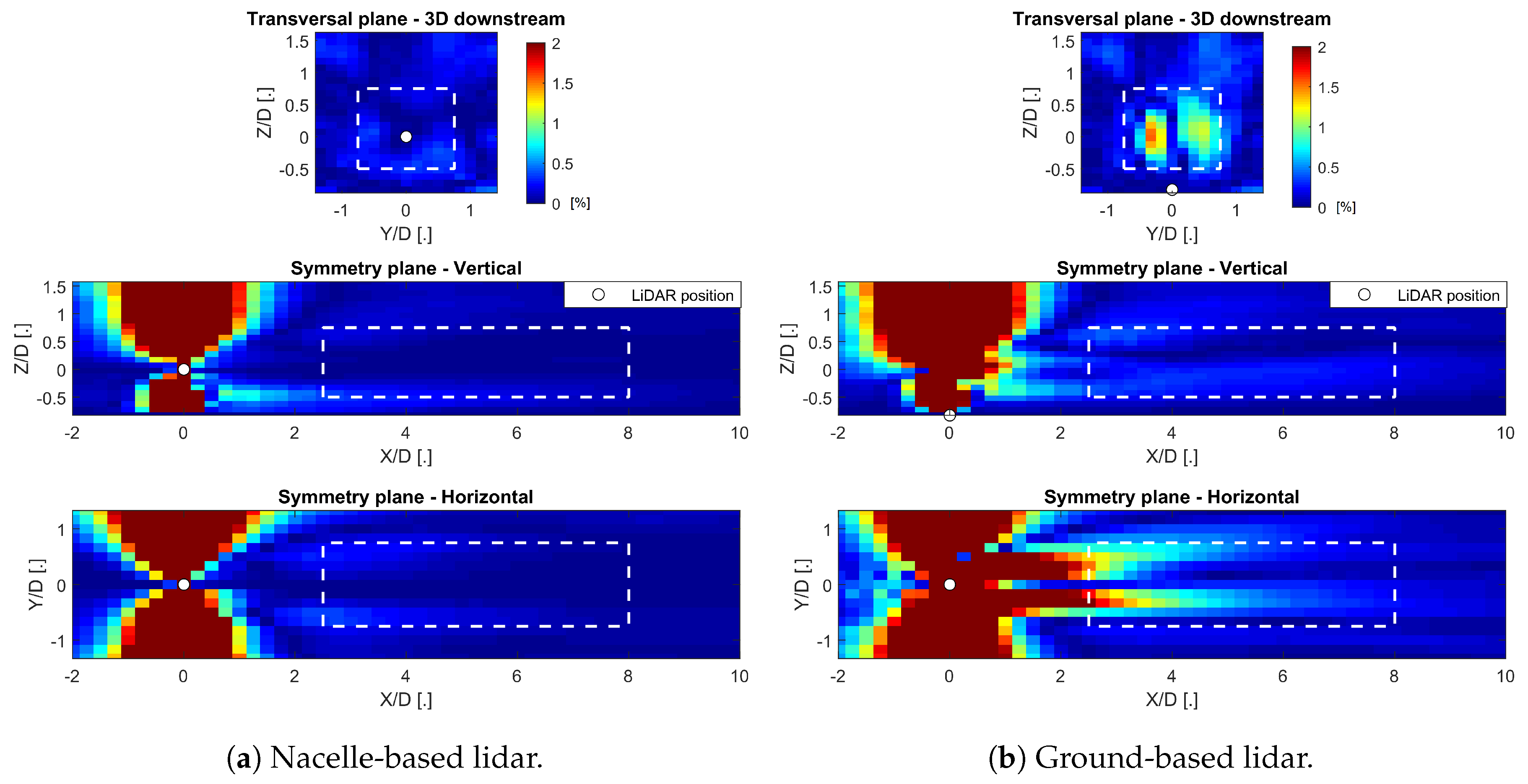
One example of error fields for the inflow case MV-MT is shown in Figure 3 for a nacelle-mounted lidar and for a ground-based lidar situated at the base of the tower. The origin of the error within the volume of interest can be divided into two: first, the deviation from the assumption of unidirectional average flow (i.e., non-zero spanwise and vertical average velocity components), which is greater in the near wake due mostly to the tangential induction of the rotor, and, second, the angle between the laser beam orientation and the x axis (given by $\phi$ and $\theta$), whose magnitude is larger for those points at the most upstream outer edges of the region of interest, and it is smaller for the nacelle-mounted lidar case. Therefore, it is easy to notice that the errors are greater when measuring with a ground-based lidar, and it is particularly well illustrated in the transversal planes at a downstream distance of 3D, as shown in Figure 3a,b . While the $\overline{v}$ and $\overline{w}$ components are the same in both cases, a ground-based lidar requires higher elevation angles ($\theta$). This is responsible for errors reaching up to 1.5%, while for the nacelle-based lidar they never exceed 0.25%.

Table 3. Errors in the reconstruction of the average longitudinal velocity component associated only with the assumption of unidimensional flow. The errors are presented for the different inflow cases studied in terms of average and maximum values found within the volume of interest (see Section 2.3 and white dashed lines in Figure 3) for both nacelle-mounted and ground-based lidars. Percentages are based on the undisturbed wind speed at hub height (see Section 2.1.3).

	Average Error [%]		Maximum Error [%]
	Nacelle	Ground	Nacelle	Ground
MV-MT	0.09	0.29	0.29	1.73
MV-LT	0.10	0.29	0.28	1.87
MV-HT	0.12	0.24	0.59	1.23
LV-MT	0.16	0.25	0.72	1.47
HV-LT	0.06	0.22	0.30	1.44

shows the errors associated with the assumption of unidirectional average flow for the five different inflow cases studied and for both nacelle-mounted and ground-based lidars. The table shows average and maximum errors for the volume of interest already defined in Section 2.3. It is possible to extract three main conclusions from it:

• The assumption of unidirectional average flow when reconstructing the average longitudinal component of the wind velocity $\overline{u}$ is a good approximation, because of the low average and maximum errors, for the study of the far wake for all inflow cases and both lidar locations.
• The nacelle-mounted lidar yields lower average and maximum errors (between two and five times lower) than the ground-based lidar situated at the bottom of the tower.
• Different inflow conditions do not affect significantly the relative magnitude of the error associated with the assumption of unidirectional average flow.

From the results presented in this section, it can be concluded that the best option to minimize only the error associated with the assumption of unidimensional average flow is to use a nacelle-mounted lidar, although it does not give a very significant advantage since both lidar positions provide acceptably low errors for most analysis purposes.

3.1.2. Total Error

The total error includes, on top of the error discussed in the previous section, the effects of the limited number of samples for statistics calculations and the error made when interpolating back from a spherical grid to a Cartesian one. The calculation of the total error follows these steps:

• For a given lidar position (nacelle or ground) the range of maximum and minimum values of the azimuth $\phi$ and elevation $\theta$ angles is calculated. Then, for a given angular resolution, the laser beam performs consecutive PPI scans until the end of the 30 min periods. This determines the evolution of the elevation and azimuth angles in time $\theta \left(t\right)$ and $\phi \left(t\right)$. The number of repetitions or samples for each orientation is shown in Table 2.
• For each time step, the virtual lidar measurement is simulated by calculating the radial velocity $Vr$ at each point along the laser beam using Equation (1).
• The average of the radial velocity is calculated at each point in space in which the virtual lidar obtains the measurements, creating a spherical regular grid with its origin at the lidar location $\overline{Vr}(\phi ,\theta ,r)$.
• The assumption of unidirectional average flow is used to calculate the average longitudinal component of the wind speed $\overline{u}(\phi ,\theta ,r)$ as shown in Equation (2).
• The data in the spherical grid are interpolated linearly to the original Cartesian grid to obtain $\overline{u}(x,y,z)$.
• The difference between the reconstructed $\overline{u}(x,y,z)$ and the same variable obtained from the original LES results conforms the error at each point in space. The average and maximum values of the error inside the volume of interest are computed.

The statistical uncertainty of the average of the radial velocity is inversely proportional to the square root of the number of independent samples $\sqrt{N}$ [46]. Since the measurement frequency of the lidar has an upper limit, a higher angular resolution means fewer measurements at each point in space for a given period and vice versa. Thus, a higher angular resolution yields a lower interpolation error, but a higher statistical error. This holds true until the time between measurements at each point in space approaches the integral time scale, which is considered the time between statistically independent measurements. It must be noted, though, that samples along the same laser beam are correlated, and those corresponding to the same PPI scans are unlikely to be independent of each other since they are consecutive measurements in time.

The linear interpolation error, in turn, is proportional to the gradient of the spatial derivative of the average flow field and proportional to the distance between the measurement points of the spherical grid. The horizontal gradient of the wind speed is greater close to the wind turbine, while the distance between measurement points increases with increasing distance to the lidar location and decreasing angular resolution.

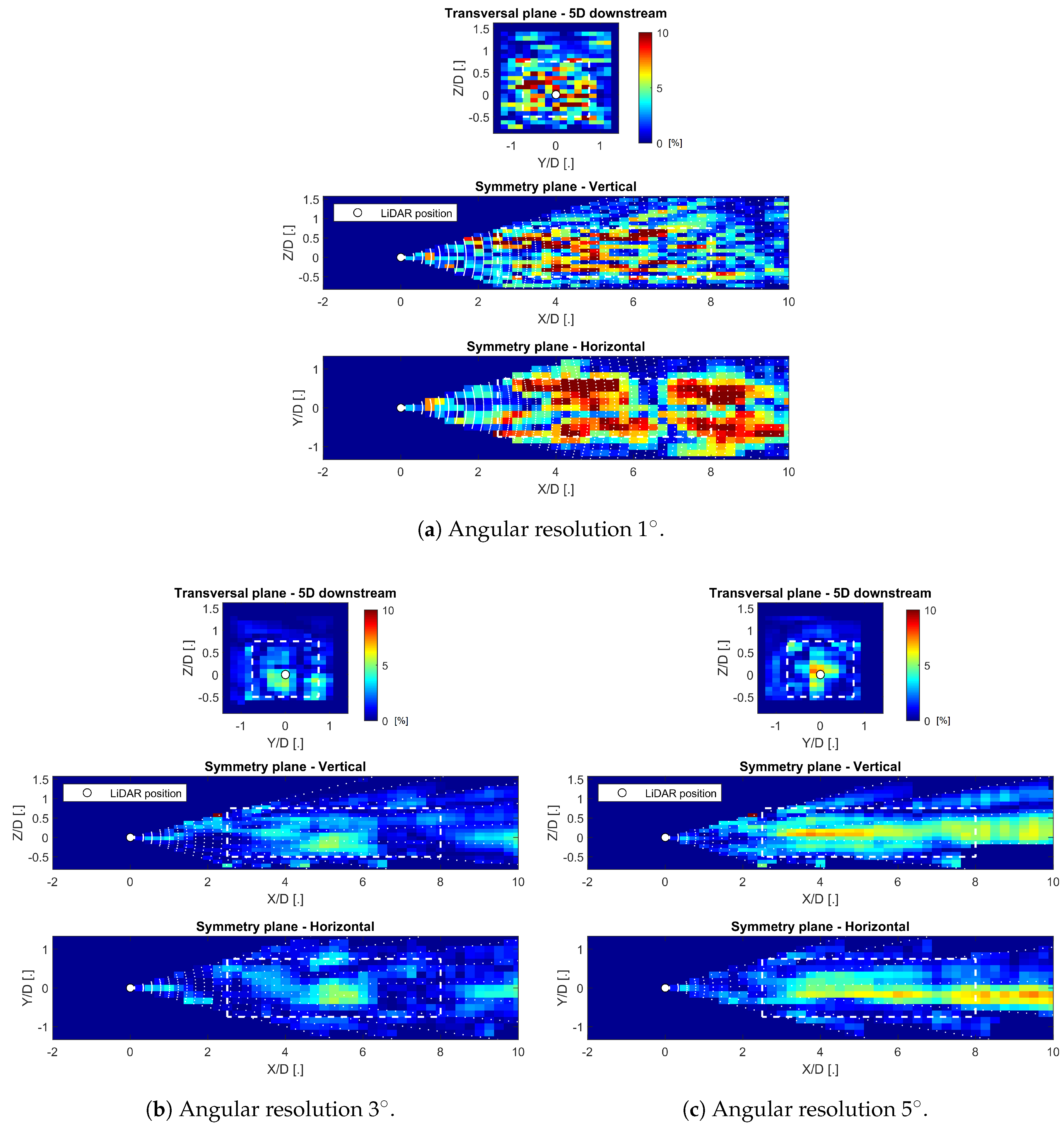
Figure 4 shows an example of the total errors for different angular resolutions for the case MV-MT and a nacelle-based lidar. The first noticeable fact is that the angular resolution of 3${}^{\circ }$ (Figure 4b) shows the lowest errors and therefore is a good compromise between angular resolution and the number of samples or repetitions at each point. On the other hand, a resolution of 1${}^{\circ }$ (Figure 4a) shows a high statistical error, evident by the fact that the errors are randomly distributed (except in the horizontal plane, since it is based on the same PPI scan as explained above), while a resolution of 5${}^{\circ }$ (Figure 4c) shows a high interpolation error, visible between the white dots that represent the points at which the virtual lidar takes measurements and from which interpolation then takes place (this is most noticeable at approximately Z/D= 0.1 and Y/D = −0.1).

Table 4. Example of optimization of the angular resolution for one inflow case and both lidar locations. The table presents the average and maximum total errors for the reconstruction of the average longitudinal velocity component inside the volume of interest. The errors are shown as a percentage of the undisturbed wind speed at hub height (see Section 2.1.3).

Angular Resolution	1${}^{\circ }$	1.5${}^{\circ }$	2${}^{\circ }$	2.5${}^{\circ }$	3${}^{\circ }$	4${}^{\circ }$	5${}^{\circ }$
	MV-MT nacelle-mounted
Average error [%]	5.2	2.6	1.6	1.8	1.5	1.7	2.5
Maximum error [%]	18.6	12.2	5.8	6.9	5.4	5.7	8.0
	MV-MT ground-based
Average error [%]	4.7	2.5	1.7	1.7	1.6	1.8	2.5
Maximum error [%]	18.9	15.3	7.7	7.8	6.3	6.9	8.5

presents an example of an optimization of the angular resolution for the inflow case MV-MT for both lidar locations. As discussed in the previous paragraphs, when scanning the wake with either a high angular resolution (1${}^{\circ }$) or a low one (5${}^{\circ }$), the errors are greater than when using a compromise resolution. The optimum value in the two cases presented is 3${}^{\circ }$, which balances the statistical errors and the interpolation errors. An extension of this table for all inflow cases studied is presented in Appendix A,

Table A1. Total average and maximum errors for the reconstruction of $\overline{u}(x,y,z)$ inside the volume of interest for all inflow cases studied and both lidar locations. The errors are shown as a percentage of the undisturbed wind speed at hub height (see Section 2.1.3). The errors corresponding to an optimum angular resolution for each case are identified with an asterisk.

Angular Resolution	1${}^{\circ }$	1.5${}^{\circ }$	2${}^{\circ }$	2.5${}^{\circ }$	3${}^{\circ }$	4${}^{\circ }$	5${}^{\circ }$	1${}^{\circ }$	1.5${}^{\circ }$	2${}^{\circ }$	2.5${}^{\circ }$	3${}^{\circ }$	4${}^{\circ }$	5${}^{\circ }$
	MV-MT nacelle-mounted							MV-MT ground-based
Average error [%]	5.2	2.6	1.6	1.8	1.5 *	1.7	2.5	4.7	2.5	1.7	1.7	1.6 *	1.8	2.5
Maximum error [%]	18.6	12.2	5.8	6.9	5.4 *	5.7	8	18.9	15.3	7.7	7.8	6.3 *	6.9	8.5
	MV-LT nacelle-mounted							MV-LT ground-based
Average error [%]	3.9	2.4	2.5	1.7 *	1.9	2.5	3.7	3.4	2.4	2.4	1.9 *	2	2.5	3.6
Maximum error [%]	17.2	10.7	12.1	5.2 *	7.1	8.5	11.7	21.9	10.4	11.2	7.3 *	7.6	8.9	11.5
	MV-HT nacelle-mounted							MV-HT ground-based
Average error [%]	5.8	3.3	2.5	2.1	1.4	1.3 *	1.5	6.2	3.6	3	1.8	1.8	1.3 *	1.5
Maximum error [%]	21.7	20.7	10.6	7.1	5.7	5 *	12.6	26.9	15.6	11.2	6.3	6.5	5.9 *	6.6
	LV-MT nacelle-mounted							LV-MT ground-based
Average error [%]	4.6	3.5	2.8	2	1.6	1.4 *	2.2	4.4	3.8	2.7	2.5	1.5 *	1.6	2.3
Maximum error [%]	24.8	21.2	11	7.5	5.8 *	6.3	9	20.7	18	11.7	11.2	7	6.2 *	8.8
	HV-MT nacelle-mounted							HV-MT ground-based
Average error [%]	4.1	3.3	2	1.8	1.7	1.6 *	2.3	4.7	2.6	2.2	1.8	1.4*	1.7	2.2
Maximum error [%]	28.7	17.6	8.3	8.6	5.4 *	6.3	9.2	18	13.2	9.6	7.4	6.6	6.1 *	8.7

, where it is possible to identify the optimum angular resolution for each case. For most cases, the optimum value is still 3${}^{\circ }$, while for a few cases it is 2.5${}^{\circ }$ or 4${}^{\circ }$, although the error is not significantly sensitive in this range of angular resolutions. It can therefore be concluded that 3${}^{\circ }$ is the overall optimum angular resolution.

Table 5. Total average and maximum errors for the reconstruction of $\overline{u}(x,y,z)$ inside the volume of interest for all inflow cases studied and both lidar locations with the overall optimum angular resolution of 3${}^{\circ }$. The errors are shown as a percentage of the undisturbed wind speed at hub height (see Section 2.1.3). The optimum values found in Table 4 correspond to the first column of this table.

	Nacelle-Mounted
	MV-MT	MV-LT	MV-HT	LV-MT	HV-MT
Average error [%]	1.5	1.9	1.4	1.6	1.7
Maximum error [%]	5.4	7.1	5.7	5.8	5.4
	Ground-Based
	MV-MT	MV-LT	MV-HT	LV-MT	HV-MT
Average error [%]	1.6	2.0	1.8	1.5	1.4
Maximum error [%]	6.3	7.6	6.5	7.0	6.6

shows the error associated with each inflow case when using an optimum angular resolution of 3${}^{\circ }$. It can be seen that the errors are reasonably low for most analysis purposes and similar for all inflow cases. Contrary to what is discussed in Section 3.1.1, the nacelle-mounted and ground-based lidars show similar results when considering the total error.

Four main conclusions can be derived from all the information presented in this section:

• An optimum angular resolution which balances the statistical error and the interpolation error can be found.
• The optimum angular resolution is nearly the same for all inflow cases and both lidar locations, and the overall optimum value is 3${}^{\circ }$.
• Different inflow cases or lidar locations do not affect significantly the optimized total error.
• The total errors found inside the volume of interest are low (average error smaller than 2% and maximum error lower than 8%), which are deemed acceptable for most applications.

3.2. Error of the Standard Deviation of the Longitudinal Velocity Component

The total error of the reconstruction of the standard deviation of the longitudinal velocity component includes the error of the assumption detailed in Equation (4), the statistical error, and the interpolation error. The calculation follows the same steps presented in Section 3.1.2, except for Point 3, where ${\sigma }_{Vr}(\phi ,\theta ,r)$ is calculated instead of $\overline{u}(\phi ,\theta ,r)$, and Point 4, in which Equation (4) is used instead of Equation (2). The same considerations regarding the statistical uncertainty and the interpolation error explained previously are also valid for the reconstruction of the standard deviation of the longitudinal velocity component.

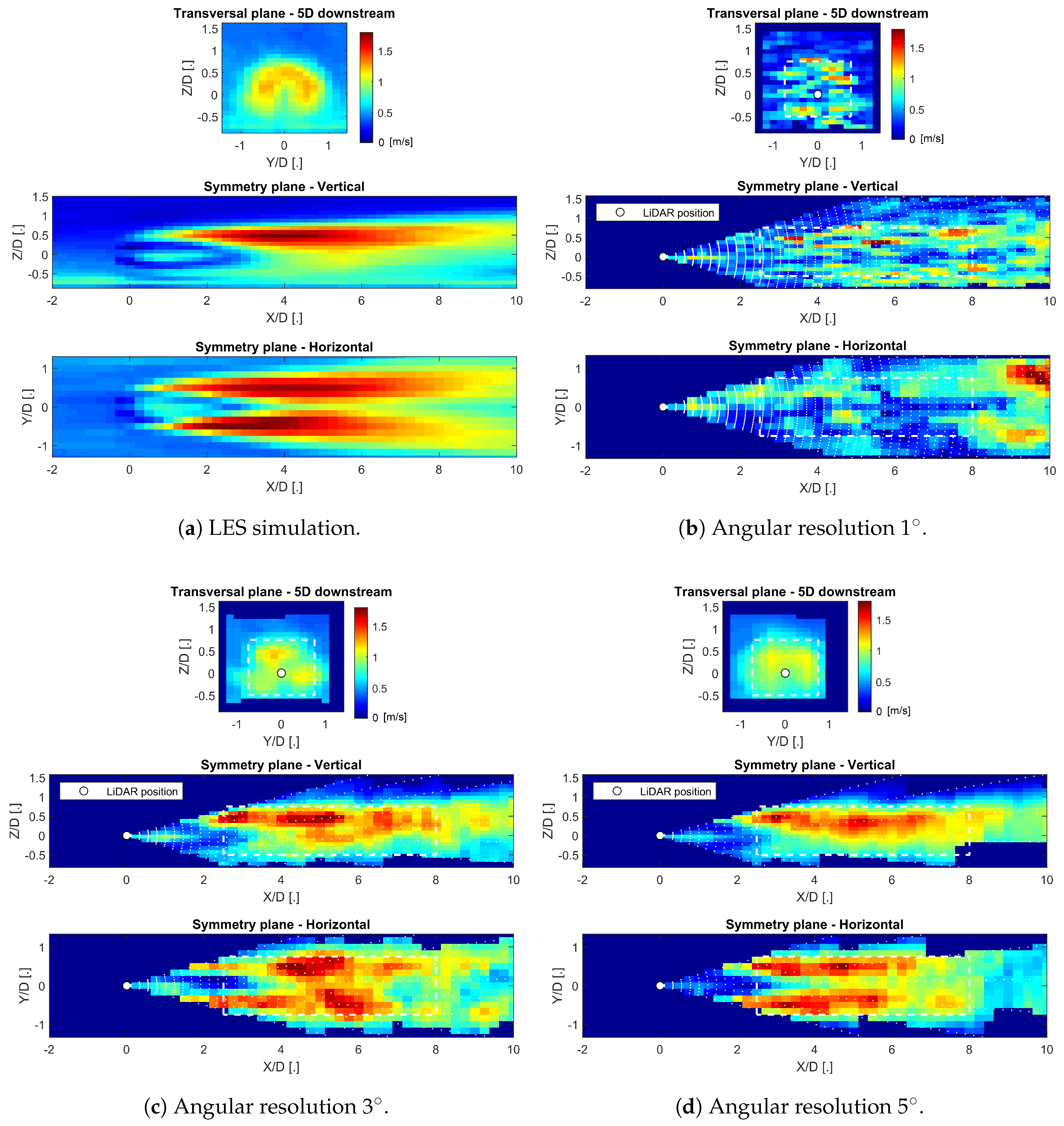
Figure 5 illustrates the impact of the total error on the reconstruction of the standard deviation of the longitudinal velocity component field ${\sigma }_u(x,y,z)$ for different angular resolutions for the case MV-MT and the nacelle-based lidar. It must be noted that, in this figure, for the sake of clarity, the magnitude of ${\sigma }_u(x,y,z)$ is used instead of the error. It can be seen that a high angular resolution (Figure 5b) results in a poor performance, while coarser resolutions (Figure 5c,d) yield visibly lower errors.

All the errors associated with each inflow case and both lidar locations are shown in Appendix A,

Table A2. Total average and maximum errors for the reconstruction of ${\sigma }_u(x,y,z)$ inside the volume of interest for all inflow cases studied and both lidar locations. The errors are shown as a percentage of the undisturbed wind speed at hub height (see Section 2.1.3). The errors corresponding to an optimum angular resolution for each case are identified with an asterisk.

Angular Resolution	1${}^{\circ }$	1.5${}^{\circ }$	2${}^{\circ }$	2.5${}^{\circ }$	3${}^{\circ }$	4${}^{\circ }$	5${}^{\circ }$	1${}^{\circ }$	1.5${}^{\circ }$	2${}^{\circ }$	2.5${}^{\circ }$	3${}^{\circ }$	4${}^{\circ }$	5${}^{\circ }$
	MV-MT nacelle-mounted							MV-MT ground-based
Average error [%]	5.5	2.9	2.2	2.0	1.9 *	2.0	2.1	5.2	3.2	2.5	2.4	2.4	2.2 *	2.5
Maximum error [%]	15.0	11.9	8.5	6.6	6.0	5.0 *	5.3	14.6	11.3	9.8	8.8	7.1	6.4 *	6.5
	MV-LT nacelle-mounted							MV-LT ground-based
Average error [%]	4.2	3.1	2.5	1.7 *	1.7 *	1.9	2.1	4.4	2.7	2.8	2.0 *	2.0 *	2.0 *	2.3
Maximum error [%]	12.7	9.2	8.8	6.4 *	6.4 *	6.7	7.7	13.5	9.3	8.3	7.2	6.5	6.4 *	7.2
	MV-HT nacelle-mounted							MV-HT ground-based
Average error [%]	6.3	3.6	2.9	2.0	1.9	1.7 *	2.0	6.9	3.9	3.6	2.8	2.9	2.6 *	2.7
Maximum error [%]	19.8	12.8	11.5	8.1	6.7	6.1	5.4 *	19.6	13.3	13.4	9.4	8.9	7.2 *	8.2
	LV-MT nacelle-mounted							LV-MT ground-based
Average error [%]	5.3	3.5	2.8	2.3	2.0 *	2.1	2.3	5.9	3.8	2.8	2.7	2.5	2.4 *	2.7
Maximum error [%]	16.0	12.2	9.2	7.2	8.0	7.2	6.8 *	16.8	13.4	11.0	10.0	8.1	7.2 *	8.0
	HV-MT nacelle-mounted							HV-MT ground-based
Average error [%]	4.6	2.7	1.8	1.6 *	1.6 *	1.6 *	1.7	4.7	2.7	2.3	2.0	2.0	1.9 *	2.1
Maximum error [%]	14.2	10.8	6.7	5.6	5.7	5.7	5.1 *	13.9	9.7	8.1	5.9	5.8 *	5.9	6.0

. The minimization of the average and maximum errors found inside the volume of interest indicates that the optimum values for the angular resolution are always between 2.5 and 4${}^{\circ }$, so 3${}^{\circ }$ is chosen again as an overall optimum angular resolution.

Table 6. Total average and maximum errors for the reconstruction of ${\sigma }_u(x,y,z)$ inside the volume of interest for all inflow cases studied and both lidar locations with the overall optimum angular resolution of 3${}^{\circ }$. The errors are shown as a percentage of the undisturbed wind speed at hub height (see Section 2.1.3).

	Nacelle-Mounted
	MV-MT	MV-LT	MV-HT	LV-MT	HV-MT
Average error [%]	1.9	1.7	1.9	2.1	1.6
Maximum error [%]	6.0	6.4	6.7	7.2	5.7
	Ground-Based
	MV-MT	MV-LT	MV-HT	LV-MT	HV-MT
Average error [%]	2.4	2.0	2.9	2.5	2.0
Maximum error [%]	7.1	6.5	8.9	8.1	5.8

shows only the errors associated with an angular resolution of 3${}^{\circ }$. The errors are close in magnitude, although slightly higher, to the errors of $\overline{u}(x,y,z)$ (see Table 5). This fact might induce some confusion when comparing them. However, it should be noted that the values of ${\sigma }_u$ are significantly smaller than the values of $\overline{u}$, so the accuracy of the calculation of the standard deviations is considerably poorer than that of the mean velocity. It can also be observed that a nacelle-mounted lidar offers a slightly better performance than a ground-based one.

The findings in this section can be summarized in three main points:

• The overall optimum angular resolution for the reconstruction of ${\sigma }_u$ is also 3${}^{\circ }$.
• The reconstruction of the ${\sigma }_u(x,y,z)$ field is of worse quality than that of $\overline{u}(x,y,z)$.
• A nacelle-mounted lidar offers a slight advantage over a ground-based one.

4. Conclusions

This study exploits the potential of the virtual lidar technique to explore the uncertainty associated with a volumetric scan of the wake of a wind turbine. When performing a succession of PPI scans, an optimum angular resolution can be found that minimizes the errors when calculating the longitudinal velocity field in terms of its average and its standard deviation. This kind of analysis is important during the experiment design part, prior to a lidar measurement campaign, in order to optimize the scanning pattern. First, the optimization dictates the best way to perform the scan, and the quantification of the error estimates the expected quality of the measurements, which will determine if they are acceptable (accurate enough) or not for a particular purpose.

Our analysis has found that, when performing a volumetric scan of the far wake of an 80 m diameter wind turbine, an angular resolution close to 3${}^{\circ }$ provides the best overall results. This holds true for a lidar with a measurement frequency of 2 Hz and a spatial resolution of 18 m. The accuracy of experiments with lidars with different characteristics can be studied using the same methodology. The study has also shown that different turbulence intensity conditions and different wind speeds do not seem to affect the quality of the measurements significantly. The location of the lidar does not seem to play a significant role on the magnitude of the errors, although a nacelle-mounted lidar has a slight advantage over a ground-based one. Other practical advantages associated with a nacelle-mounted lidar, such as a constant angular orientation with the turbine rotor, are not discussed in this study.

Finally, the errors found when reconstructing the average longitudinal velocity component are low, regardless of the configuration or inflow case studied. This fact suggests that full scale measurements using the setup and data processing detailed previously should be of high quality and potentially acceptable for most applications. On the other hand, the error associated with the reconstruction of the standard deviation of the longitudinal velocity component is almost identical in magnitude to that of the average velocity, which means that, in relative terms, it is higher. This should be considered when assessing the acceptability of the lidar measurement of this variable, depending on its final purpose.

Future studies could address the effect of the thermal stability of the ABL, the wind veer, non-stationary conditions, or the horizontal inhomogeneity of the undisturbed boundary layer within the wind turbine wake region.

References

- Vermeer, L.; Sørensen, J.; Crespo, A. Wind turbine wake aerodynamics. Prog. Aerosp. Sci. 2003, 39, 467–510. [Google Scholar] [CrossRef]
- Barthelmie, R.J.; Pryor, S.C.; Frandsen, S.T.; Hansen, K.S.; Schepers, J.G.; Rados, K.; Schlez, W.; Neubert, A.; Jensen, L.E.; Neckelmann, S. Quantifying the impact of wind turbine wakes on power output at offshore wind farms. J. Atmos. Ocean. Technol. 2010, 27, 1302–1317. [Google Scholar] [CrossRef]
- Hansen, K.S.; Barthelmie, R.J.; Jensen, L.E.; Sommer, A. The impact of turbulence intensity and atmospheric stability on power deficits due to wind turbine wakes at Horns Rev wind farm. Wind Energy 2012, 15, 183–196. [Google Scholar] [CrossRef] [Green Version]
- Thomsen, K.; Sørensen, P. Fatigue loads for wind turbines operating in wakes. J. Wind Eng. Ind. Aerodyn. 1999, 80, 121–136. [Google Scholar] [CrossRef]
- Herbert-Acero, J.; Probst, O.; Réthoré, P.E.; Larsen, G.; Castillo-Villar, K. A Review of Methodological Approaches for the Design and Optimization of Wind Farms. Energies 2014, 7, 6930–7016. [Google Scholar] [CrossRef] [Green Version]
- Gebraad, P.; Thomas, J.J.; Ning, A.; Fleming, P.; Dykes, K. Maximization of the annual energy production of wind power plants by optimization of layout and yaw-based wake control. Wind Energy 2017, 20, 97–107. [Google Scholar] [CrossRef]
- Sørensen, J.N.; Shen, W.Z. Numerical Modeling of Wind Turbine Wakes. J. Fluids Eng. 2002, 124, 393. [Google Scholar] [CrossRef]
- Bastankhah, M.; Porté-Agel, F. A new analytical model for wind-turbine wakes. Renew. Energy 2014, 70, 116–123. [Google Scholar] [CrossRef]
- Crespo, A.; Hernández, J.; Frandsen, S. Survey of modelling methods for wind turbine wakes and wind farms. Wind Energy 1999, 2, 1–24. [Google Scholar] [CrossRef]
- Kocer, G.; Mansour, M.; Chokani, N.; Abhari, R.; Müller, M. Full-Scale Wind Turbine Near-Wake Measurements Using an Instrumented Uninhabited Aerial Vehicle. J. Sol. Energy Eng. 2011, 133, 041011. [Google Scholar] [CrossRef]
- Reuder, J.; Jonassen, M.O. First Results of Turbulence Measurements in a Wind Park with the Small Unmanned Meteorological Observer SUMO. Energy Procedia 2012, 24, 176–185. [Google Scholar] [CrossRef] [Green Version]
- Wildmann, N.; Hofsäß, M.; Weimer, F.; Joos, A.; Bange, J. MASC—A small Remotely Piloted Aircraft (RPA) for wind energy research. Adv. Sci. Res. 2014, 11, 55–61. [Google Scholar] [CrossRef]
- Subramanian, B.; Chokani, N.; Abhari, R. Experimental analysis of wakes in a utility scale wind farm. J. Wind Eng. Ind. Aerodyn. 2015, 138, 61–68. [Google Scholar] [CrossRef]
- Subramanian, B.; Chokani, N.; Abhari, R.S. Drone-Based Experimental Investigation of Three-Dimensional Flow Structure of a Multi-Megawatt Wind Turbine in Complex Terrain. J. Sol. Energy Eng. 2015, 137, 051007. [Google Scholar] [CrossRef]
- Käsler, Y.; Rahm, S.; Simmet, R.; Kühn, M. Wake measurements of a multi-MW wind turbine with coherent long-range pulsed doppler wind lidar. J. Atmos. Ocean. Technol. 2010, 27, 1529–1532. [Google Scholar] [CrossRef]
- Iungo, G.V.; Wu, Y.T.; Porté-Agel, F. Field measurements of wind turbine wakes with lidars. J. Atmos. Ocean. Technol. 2013, 30, 274–287. [Google Scholar] [CrossRef]
- Smalikho, I.N.; Banakh, V.A.; Pichugina, Y.L.; Brewer, W.A.; Banta, R.M.; Lundquist, J.K.; Kelley, N.D. Lidar investigation of atmosphere effect on a wind turbine wake. J. Atmos. Ocean. Technol. 2013, 30, 2554–2570. [Google Scholar] [CrossRef]
- Iungo, G.V.; Porté-Agel, F. Volumetric lidar scanning of wind turbine wakes under convective and neutral atmospheric stability regimes. J. Atmos. Ocean. Technol. 2014, 31, 2035–2048. [Google Scholar] [CrossRef]
- Banta, R.M.; Pichugina, Y.L.; Brewer, W.A.; Lundquist, J.K.; Kelley, N.D.; Sandberg, S.P.; Alvarez, R.J.; Hardesty, R.M.; Weickmann, A.M. 3D volumetric analysis of wind turbine wake properties in the atmosphere using high-resolution Doppler lidar. J. Atmos. Ocean. Technol. 2015, 32, 904–914. [Google Scholar] [CrossRef]
- Aitken, M.L.; Banta, R.M.; Pichugina, Y.L.; Lundquist, J.K. Quantifying Wind Turbine Wake Characteristics from Scanning Remote Sensor Data. J. Atmos. Ocean. Technol. 2014, 31, 765–787. [Google Scholar] [CrossRef]
- Doubrawa, P.; Barthelmie, R.; Wang, H.; Pryor, S.; Churchfield, M. Wind Turbine Wake Characterization from Temporally Disjunct 3-D Measurements. Remote Sens. 2016, 8, 939. [Google Scholar] [CrossRef]
- El-Asha, S.; Zhan, L.; Iungo, G.V. Quantification of power losses due to wind turbine wake interactions through SCADA, meteorological and wind LiDAR data. Wind Energy 2017, 20, 1823–1839. [Google Scholar] [CrossRef]
- Bodini, N.; Zardi, D.; Lundquist, J.K. Three-dimensional structure of wind turbine wakes as measured by scanning lidar. Atmos. Meas. Tech. 2017, 10, 2881–2896. [Google Scholar] [CrossRef]
- Sathe, A.; Mann, J.; Gottschall, J.; Courtney, M.S. Can Wind Lidars Measure Turbulence? J. Atmos. Ocean. Technol. 2011, 28, 853–868. [Google Scholar] [CrossRef]
- Sathe, A.; Mann, J. Measurement of turbulence spectra using scanning pulsed wind lidars. J. Geophys. Res. Atmos. 2012, 117. [Google Scholar] [CrossRef] [Green Version]
- Newman, J.F.; Clifton, A. An error reduction algorithm to improve lidar turbulence estimates for wind energy. Wind Energy Sci. 2017, 2, 77–95. [Google Scholar] [CrossRef]
- Carbajo Fuertes, F.; Iungo, G.V.; Porté-Agel, F. 3D Turbulence Measurements Using Three Synchronous Wind Lidars: Validation against Sonic Anemometry. J. Atmos. Ocean. Technol. 2014, 31, 1549–1556. [Google Scholar] [CrossRef]
- Newman, J.F.; Bonin, T.A.; Klein, P.M.; Wharton, S.; Newsom, R.K. Testing and validation of multi-lidar scanning strategies for wind energy applications. Wind Energy 2016, 19, 2239–2254. [Google Scholar] [CrossRef]
- Vasiljević, N.; Lea, G.; Courtney, M.; Cariou, J.P.; Mann, J.; Mikkelsen, T. Long-Range WindScanner System. Remote Sens. 2016, 8, 896. [Google Scholar] [CrossRef]
- Stawiarski, C.; Traumner, K.; Knigge, C.; Calhoun, R. Scopes and challenges of dual-doppler lidar wind measurements-an error analysis. J. Atmos. Ocean. Technol. 2013, 30, 2044–2062. [Google Scholar] [CrossRef]
- Stawiarski, C.; Träumner, K.; Kottmeier, C.; Knigge, C.; Raasch, S. Assessment of Surface-Layer Coherent Structure Detection in Dual-Doppler Lidar Data Based on Virtual Measurements. Bound.-Layer Meteorol. 2015, 156, 371–393. [Google Scholar] [CrossRef]
- Lundquist, J.K.; Churchfield, M.J.; Lee, S.; Clifton, A. Quantifying error of lidar and sodar doppler beam swinging measurements of wind turbine wakes using computational fluid dynamics. Atmos. Meas. Tech. 2015, 8, 907–920. [Google Scholar] [CrossRef]
- Mirocha, J.D.; Rajewski, D.A.; Marjanovic, N.; Lundquist, J.K.; Kosović, B.; Draxl, C.; Churchfield, M.J. Investigating wind turbine impacts on near-wake flow using profiling lidar data and large-eddy simulations with an actuator disk model. J. Renew. Sustain. Energy 2015, 7, 043143. [Google Scholar] [CrossRef]
- Van Dooren, M.F.; Trabucchi, D.; Kühn, M. A methodology for the reconstruction of 2D horizontal wind fields of wind turbinewakes based on dual-Doppler lidar measurements. Remote Sens. 2016, 8, 809. [Google Scholar] [CrossRef]
- Meyer Forsting, A.R.; Troldborg, N.; Murcia Leon, J.P.; Sathe, A.; Angelou, N.; Vignaroli, A. Validation of a CFD model with a synchronized triple-lidar system in the wind turbine induction zone. Wind Energy 2017, 20, 1481–1498. [Google Scholar] [CrossRef]
- Van Dooren, M.F.; Campagnolo, F.; Sjöholm, M.; Angelou, N.; Mikkelsen, T.; Floris, M. Demonstration and uncertainty analysis of synchronised scanning lidar measurements of 2-D velocity fields in a boundary-layer wind tunnel. Wind Energy Sci. 2017, 2, 329–341. [Google Scholar] [CrossRef]
- Porté-Agel, F.; Wu, Y.T.; Lu, H.; Conzemius, R.J. Large-eddy simulation of atmospheric boundary layer flow through wind turbines and wind farms. J. Wind Eng. Ind. Aerodyn. 2011, 99, 154–168. [Google Scholar] [CrossRef]
- Wu, Y.T.; Porté-Agel, F. Large-Eddy Simulation of Wind-Turbine Wakes: Evaluation of Turbine Parametrisations. Bound.-Layer Meteorol. 2011, 138, 345–366. [Google Scholar] [CrossRef]
- Wu, Y.T.; Porté-Agel, F. Modeling turbine wakes and power losses within a wind farm using LES: An application to the Horns Rev offshore wind farm. Renew. Energy 2015, 75, 945–955. [Google Scholar] [CrossRef]
- Porté-Agel, F.; Meneveau, C.; Parlange, M.B. A scale-dependent dynamic model for large-eddy simulation: application to a neutral atmospheric boundary layer. J. Fluid Mech. 2000, 415, 261–284. [Google Scholar] [CrossRef]
- Stoll, R.; Porté-Agel, F. Dynamic subgrid-scale models for momentum and scalar fluxes in large-eddy simulations of neutrally stratified atmospheric boundary layers over heterogeneous terrain. Water Resour. Res. 2006, 42, 1–18. [Google Scholar] [CrossRef]
- Wieringa, J. Updating the Davenport roughness classification. J. Wind Eng. Ind. Aerodyn. 1992, 41, 357–368. [Google Scholar] [CrossRef]
- Mikkelsen, R. Actuator Disc Methods Applied to Wind Turbines. Ph.D. Thesis, Technical University of Denmark, Lyngby, Denmark, 2003. [Google Scholar]
- Sathe, A.; Mann, J. A review of turbulence measurements using ground-based wind lidars. Atmos. Meas. Tech. 2013, 6, 3147–3167. [Google Scholar] [CrossRef] [Green Version]
- Pearson, G.; Davies, F.; Collier, C. An analysis of the performance of the UFAM pulsed Doppler lidar for observing the boundary layer. J. Atmos. Ocean. Technol. 2009, 26, 240–250. [Google Scholar] [CrossRef]
- Benedict, L.H.; Gould, R.D. Towards better uncertainty estimates for turbulence statistics. Exp. Fluids 1996, 22, 129–136. [Google Scholar] [CrossRef]
Figure 1.
Inflow conditions in terms of average horizontal wind speed and longitudinal, transversal and vertical turbulence intensity. The panels on top (a) show three cases with the same turbulence intensity (medium) but different wind speeds, while the panels at the bottom (b) show three cases with the same wind speed (medium) at hub height but different turbulence intensities. The resulting average transversal and vertical velocities from the LES simulations are negligible.
Figure 2.
Flow statistics of the simulated wind turbine wakes for the five different inflow cases studied. The figures present vertical planes at Y = 0 of the longitudinal component of the wind velocity in terms of its average (a) and its standard deviation (b). The black boxes correspond to the location of the wind turbine rotor.
Figure 3.
Example of errors in the reconstruction of the longitudinal average velocity component associated only with the assumption of unidimensional flow. The errors correspond to the MV-MT inflow case and for the lidar installed on the nacelle (a) and at the base of the tower (b). The volume of interest is delimited by the white dashed line. The figures show the error as a percentage of the undisturbed wind speed at hub height (see Section 2.1.3).
Figure 4.
Example of total errors in the reconstruction of . The errors correspond to the MV-MT inflow case with the nacelle-mounted lidar and for three different angular resolutions: 1 (a), 3 (b), and 5 (c). The volume of interest is delimited by the white dashed line, and spherical grid points are marked as white dots. The figures show the error as a percentage of the undisturbed wind speed at hub height (see Section 2.1.3).
Figure 5.
from (a) LES simulations and an example of its reconstruction using three different angular resolutions: (b) 1, (c) 3, and (d) 5. The example corresponds to the MV-MT inflow case and to the nacelle-mounted lidar. The volume of interest is delimited by the white dashed line, and spherical grid points are marked as white dots. The figures show the magnitude of in m/s.