Attribution of Flux Partitioning Variations between Land Surface Models over the Continental U.S.

Abstract

Accurate quantification of the terrestrial evapotranspiration ($ET$) components of plant transpiration (T), soil evaporation (E) and evaporation of the intercepted water (I) is necessary for improving our understanding of the links between the carbon and water cycles. Recent studies have noted that, among the modeled estimates, large disagreements exist in the relative contributions of T, E and I to the total $ET$. As these models are often used in data assimilation environments for incorporating and extending $ET$ relevant remote sensing measurements, understanding the sources of inter-model differences in $ET$ components is also necessary for improving the utilization of such remote sensing measurements. This study quantifies the contributions of two key factors explaining inter-model disagreements to the uncertainty in total $ET$: (1) contribution of the local partitioning and (2) regional distribution of $ET$. The analysis is conducted by using outputs from a suite of land surface models in the North American Land Data Assimilation System (NLDAS) configuration. For most of these models, transpiration is the dominant component of the $ET$ partition. The results indicate that the uncertainty in local partitioning dominates the inter-model spread in modeled soil evaporation E. The inter-model differences in T are dominated by the uncertainty in the distribution of $ET$ over the Eastern U.S. and the local partitioning uncertainty in the Western U.S. The results also indicate that uncertainty in the T estimates is the primary driver of total $ET$ errors. Over the majority of the U.S., the contribution of the two factors of uncertainty to the overall uncertainty is non-trivial.

1. Introduction

Evapotranspiration ($ET$) is a key component of the terrestrial water cycle and it plays a critical role in the climate system by regulating the land-atmosphere fluxes and feedbacks ([1,2]). As a result, there have been several community efforts to quantify the global and regional uncertainties in estimating $ET$ in land surface models and remote sensing-based measurements ([3,4,5,6,7]). These studies demonstrated that patterns of seasonality and spatial distribution of $ET$ across climate regimes are generally well captured by the $ET$ products, though uncertainty still remains in the total $ET$ estimates ([4]).

By comparison, less attention has been paid to studying the uncertainty in partitioning of $ET$ into its source components: transpiration (T), soil evaporation (E) and canopy evaporation of intercepted rainfall (I). In particular, the partitioning between T and E is key to an accurate coupling of water and carbon cycles and a variety of water and agricultural management applications ([8,9]). T, documented to be the main component of the global $ET$ ([10,11]), is influenced by stomatal control in response to water stress. Both E and T occur in response to atmospheric evaporative demand and are limited by water availability. The main difference is that T is further affected by vegetation growth and stomatal control. The lower albedo and the differences in aerodynamic conductance associated with vegetation also have significant impacts on the available energy for T. Furthermore, whereas water availability for E is determined by the surface soil moisture, accessible water for T is determined by the rooting depth. The result is that these two processes exhibit different rates of response to the same water and energy inputs (precipitation and solar radiation). I is primarily influenced by precipitation (in particular, rainfall frequency and rainfall rate) and vegetation characteristics ([12]). Improvements in the characterization of I will benefit catchment-scale water balance applications as it bypasses the soil reservoir entirely. One reason for the lack of a thorough understanding of the $ET$ partition is the fact that in situ global measurements of the $ET$ components are very sparse ([13]). Several studies use process-based model formulations informed by remote sensing datasets to quantify the uncertainty in the $ET$ partition ([7,8,14,15]). These studies confirm the dominant role of transpiration over vegetated and wet regions and soil evaporation over dry regions, in influencing $ET$. The outputs from land surface models (LSMs) driven by observation-based meteorology are also often used for deriving estimates of $ET$ components. Recent studies have noted large disagreements in the relative distributions of T, I and E ([3,7,16]). This disagreement exists both between LSMs ([3]) and in process-based $ET$ retrievals ([7]). As direct measurements of $ET$ and $ET$ components are not available from remote sensing instruments, such model formulations are critical in translating the relevant measurements to geophysical variables. Furthermore, these models are the basis of data assimilation environments that help to extend the spatial and temporal coverage of the typically discontinuous remote sensing measurements. As a result, understanding and quantifying the differences in the modeled estimates of $ET$ components is important for improving the utilization of available remote sensing information.

Prior studies have suggested that the source of uncertainty in the relative distributions of the $ET$ components limits the ability of the models to provide sensitivities of $ET$ to precipitation deficits and land cover change, which in turn impacts the ability of the models to predict the progression of extreme events such as droughts ([17,18]). Although the reported disagreements in the ratio of T to $ET$ have placed a spotlight on key process descriptions affecting the global $ET$ partitioning estimates, the global aggregations make it somewhat difficult to interpret. For example, even if two different LSMs have the same (time-integrated) T fraction at each model grid cell, they can yield different fractions in their global comparisons if they do not agree on the distribution of total $ET$ between T dominated regions and E dominated regions. The opposite can also occur; differences in local grid-level partitioning can be masked by differences in regional distribution. It is important to distinguish between these two alternative explanations (local partitioning vs regional distribution of total $ET$) so that efforts to improve the LSMs can be directed appropriately. Note that these two factors are analogous to examining the impact of absolute and relative magnitudes of $ET$ components.

In this study, we explore the level of agreement in $ET$ partitioning for the continental U.S. using outputs from a suite of LSMs implemented in the North American Data Assimilation System (NLDAS; [19]) configuration. NLDAS is a multi-institution effort, which runs four LSMs operationally (Noah version 2.8, [20,21,22]; Mosaic, [23,24]; Variable Infiltration Capacity (VIC) version 4.0.3, [25]; and Sacramento Soil Moisture Accounting (SAC), [26]) using observation-based meteorological data. More recent efforts have focused on upgrading the current suite of NLDAS models ([27]). We use the outputs from both the operational NLDAS Phase 2 (NLDAS-2) and from four additional models planned for the next phase of NLDAS (Noah version 3.6, [28,29]; Catchment LSM, [30,31]; VIC version 4.1.2l, [32]; and a configuration of Noah-MP, [33,34]) in the NLDAS-2 configuration. The version of SAC used in NLDAS-2 does not compute surface flux partition estimates and therefore is not included in this study. For these models, we examine the domain-wide and regional breakdown of the $ET$ partitioning to determine whether the overall disagreement stems from local flux partitioning or variations in the regional distribution of total $ET$. Specifically, this paper examines the sources of disagreements in bulk partitioning. In addition, the ensemble model outputs are used to estimate the uncertainty in the flux partitioning and how the uncertainty varies spatially across the Continental U.S. (CONUS) domain.

2. Models

LSM simulations using the seven models are conducted over the NLDAS-2 domain, which spans from 25${}^{\circ }$N to 53${}^{\circ }$N and 125${}^{\circ }$W to 67${}^{\circ }$W on a 0.125${}^{\circ }$ lat by 0.125${}^{\circ }$ lon grid. Model outputs over an 11-year time period (from January 2002 to December 2012) are considered in this study. All models are forced with the same NLDAS-2 meteorology data (Xia et al. [19]) with a 15-min timestep (except for both versions of VIC, which use an hourly timestep).

Generally, all LSMs considered here follow the Penman–Monteith (P–M) approach with different model parameterizations for $ET$ relevant computations. In the Noah model formulations, the P–M approach is used for computing potential evapotranspiration ($PET$), which is then used for computing E and T. E is modeled by scaling $PET$ as a function of soil moisture availability and fractional vegetation coverage ([35]). Similarly, a plant coefficient term, canopy water content and fractional vegetation are used to scale the $PET$ for computing T. The plant coefficient term represents the effects of the stomatal control and is formulated to include canopy resistance factors representing the effects of solar radiation, vapor pressure deficit, air temperature and soil moisture. The canopy resistance computations are based on [36] in Noah28 and Noah36, whereas NoahMP uses a dynamic vegetation formulation based on [37]. The canopy interception contribution to $ET$ in these models is a function of the interception reservoir, which is modeled as a function of either the Leaf Area Index (LAI) or fractional vegetation.

Similar to Noah, the E and T in VIC are calculated by scaling the $PET$, which is calculated using a modified P–M equation ([38]). A Jarvis-style formulation is used to model the stomatal resistance, as a function of air temperature, vapor pressure deficit and photosynthetically active radiation. A distinct feature of VIC is that the soil evaporation is dependent on the non-vegetated areas only (i.e., it does not explicitly consider evaporation from soil underlying vegetation).

The Catchment LSM (CLSM) employs a non-traditional approach where the subgrid heterogeneity in soil moisture is statistically represented by subdividing the land portion of the grid cell into three distinct regions: (1) a saturated region where evaporation occurs without the consideration of water stress; (2) a subsaturated region where transpiration occurs with limited water stress and (3) a wilting region where transpiration is completely shut off. The relative weights for these three regions are defined as functions of the local topography and soil water prognostic variables. The energy balance formulations in CLSM are derived from that of the Mosaic model (which has a traditional layered soil moisture structure). In both CLSM and Mosaic, the transpiration formulations follow the model of [39]. More detailed description of the model physics formulations of these models is provided in [27].

All of the LSMs use the University of Maryland’s UMD Land Cover classification, which was derived from the Advanced Very High Resolution Radiometer (AVHRR) satellite imagery between 1981 and 1994 to create a static land cover map. This classification uses 13 vegetation types, plus one for water. Most of the LSMs (e.g., Noah, Noah-MP) were able to use these types directly, while, in some cases (e.g., CLSM), a mapping was performed between the UMD vegetation classes and the classes specific to that model. The state soil geographic (STATSGO) soil database ([40]) is used to specify the soil texture types in the model configurations. Monthly vegetation climatologies of the fraction of green vegetation (GVF) and/or LAI were used, depending on the model, although all models used the same or very similar source for these vegetation datasets. The one exception is that the Noah-MP LSM, as configured for this study, used the dynamic vegetation module, which simulates the masses (leaf, stem, root, etc.) of the vegetation prognostic variables and calculates the GVF/LAI instead. The key details of the model configurations are summarized in

Table 1. Configuration of the model simulations used in this study. NLDAS—North American Land Data Assimilation System; CLSM—Catchment land surface model; VIC—variable infiltration capacity; AVHRR—Advanced Very High Resolution Radiometer; UMD—University of Maryland; STATSGO—state soil geographic; LAI—leaf area index; GVF—green vegetation fraction.

Model domain	Continental U.S.
	(25${}^{\circ }$N to 53${}^{\circ }$N and 125${}^{\circ }$W to 67${}^{\circ }$W)
Spatial resolution	0.125${}^{\circ }$
Forcing input	NLDAS-2 data
Timestep (Noah (2.8, 3.6, MP), Mosaic, CLSM)	15 min
VIC (4.0.3, 4.1.2.l)	1 h
Landcover	AVHRR-based UMD land cover classification
Soils	STATSGO soil texture
LAI/GVF (except Noah-MP)	AVHRR-based climatology

.

3. Methods

The analysis of CONUS wide partitioning of $ET$ is based on the multiyear average annual flux attributed to the three source components (S referring to T, E or I). For each model m, the fraction of total $ET$ is calculated for each source component ($F(S)$) as the summation over space (x representing the grid cell):

$$F{(S)}_m=\frac{{\Sigma }_x{S}_{x,m}}{{\Sigma }_x(E_{x,m}+T_{x,m}+I_{x,m}).}$$

(1)

This summation is used in most prior studies [3,7] to quantify the uncertainties in global $ET$ partitioning. Note that no correction for latitudinal differences are included in the areal summation of these terms. To investigate the level of agreement in $F(S)$ between models over the spatial domain, we also calculate the fractional contribution of the three evaporation sources at each grid cell location x:

$$F{(S)}_{m,x}=\frac{S_{x,m}}{(E_{x,m}+T_{x,m}+I_{x,m}).}$$

(2)

Because $F{(S)}_m$ Equation (1) is not the domain average of the $F{(S)}_{m,x}$ Equation (2), this by itself may not explain the differences in the domain-wide $ET$ partition ($F{(S)}_m$). To identify the source of inter-model disagreement in the ratios of each component over total $ET$, we analyze two potential sources of discrepancy: (1) the uncertainty in the fractional partition across the models and (2) the uncertainty in the total $ET$ in the models and how it influences the magnitude of the $ET$ components. We therefore define two measures that isolate the contribution of these factors, as follows:

The first term, the contribution of the partitioning uncertainty to the uncertainty in total domain partitioning ($C_P$) is defined as:

$$C_P{(S)}_x=\mathbf{mean}[(E_{x,m}+T_{x,m}+I_{x,m})]\times \mathbf{stdev}[(F{(S)}_{m,x})],$$

(3)

where the $\mathbf{mean}$ and $\mathbf{stdev}$ represent the multi-model mean and standard deviation, respectively.

This contribution can be contrasted with the second term, the contribution of uncertainty in total $ET$ ($C_{ET}$) to the partitioning, defined as:

$$C_{ET}{(S)}_x=\mathbf{stdev}[\frac{(E_{x,m}+T_{x,m}+I_{x,m})}{G_m}]\times \mathbf{mean}[(F{(S)}_{m,x})],$$

(4)

where $G_m$ is the total ‘gain’ for each model represented by:

$$G_m=\frac{{\Sigma }_x(E_{x,m}+T_{x,m}+I_{x,m})}{\mathbf{mean}[{\Sigma }_x(E_{x,m}+T_{x,m}+I_{x,m})].}$$

(5)

The gain term corrects for the mean bias in total $ET$ across the domain for each model, which does not affect the domain-wide partitioning obtained through Equation (1). Essentially, $C_P$ is defined by scaling the average total $ET$ across the models by the standard deviation of the fractional $ET$ partition, whereas $C_{ET}$ is defined by scaling the variability in the total $ET$ by the average fractional $ET$ partition. Thus, $C_P$ and $C_{ET}$ terms highlight the contributions of the uncertainty in fractional partitioning, and contributions of the uncertainty in total $ET$ to the inter-model differences in the T, E and I estimates, respectively. The patterns in $C_P$ and $C_{ET}$ can be used to figure out where the model development efforts to improve the $ET$ components should be focused.

4. Results and Discussion

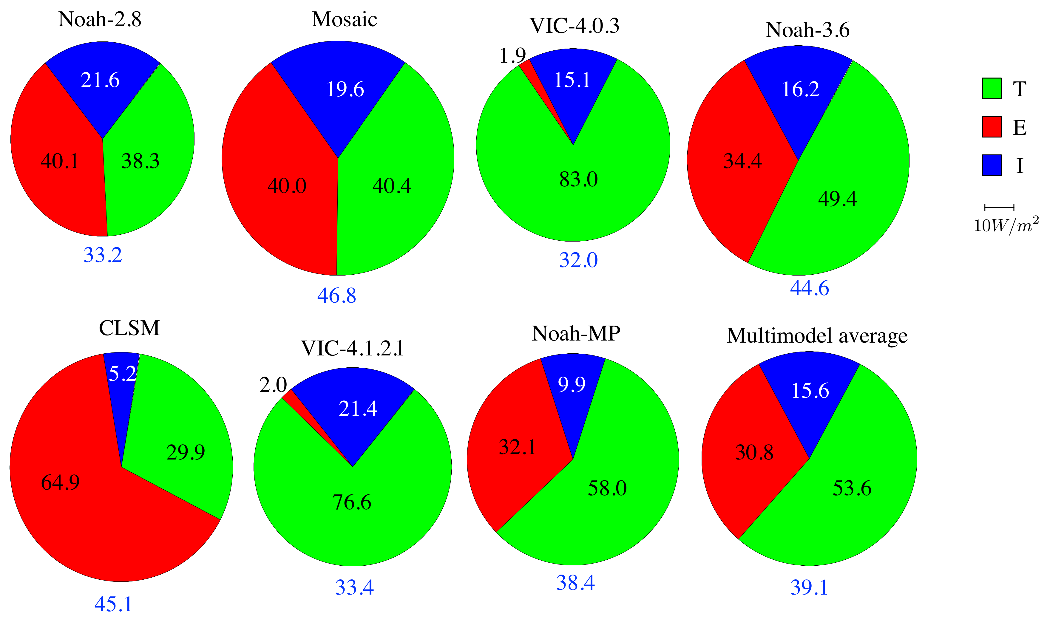
Figure 1 shows the domain averaged partition using Equation (1) for the seven models that are employed in this study. Note that the circles are scaled in proportion to the domain averaged $ET$ estimate from each model. The variation in size shows that there is significant uncertainty across the models in the domain averaged $ET$, even though all of them employ the same forcing data, landcover, soils and topography information. In addition, there are significant disagreements in the domain-wide $ET$ partitioning. Consistent with the literature, the T component is the dominant source of $ET$ in most models except in case of CLSM, while the T and E are roughly equal in Noah-2.8 and in Mosaic. The $ET$ partitioning is particularly different in both versions of VIC, where E is the smallest of the three components and T constitutes most of the total $ET$, likely due to the fact that VIC does not employ time varying vegetation information for computing E. The multimodel mean estimate of $ET$ partitioning is 53.6% for T, 30.8% for E and 15.6% for I, which shows a slightly higher portion of T relative to E than the multimodel averages reported by the Global Soil Wetness Project-2 (48% for T, 36% for E and 16% for I; [3]). In situ and process model-based partitioning studies have reported significantly different estimates for the T and E partitions. Using partitioning estimates derived from eddy-covariance, sap-flow and isotopic approaches, Ref. [11] reports the relative contributions of T and E to total $ET$ to be at 61% (±15%) and 39% (±10%), respectively. Similarly, Ref. [7] indicates that the T fraction of total $ET$ vary between 24% to 76% and that of E vary between 14% to 26% from three different process-based evaporation methodologies.

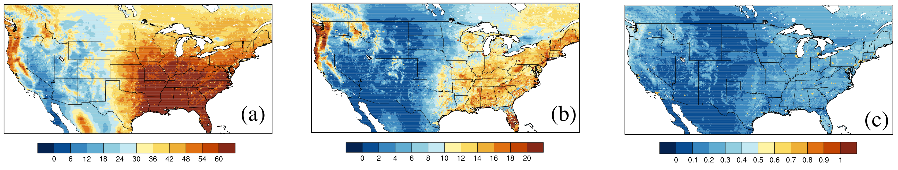
The spatial distribution of the $ET$ and the $ET$ partition is examined in Figure 2 and Figure 3. As shown in Figure 2, the mean and standard deviation of $ET$ is higher in the Eastern U.S. and lower in the Western U.S., indicating that the absolute differences among the models is high over the Eastern U.S. The coefficient of variation (CV; ratio of standard deviation to the mean) of total $ET$ also indicates that the relative variability of total $ET$ is higher in the Eastern U.S., compared to the West. This is consistent with prior multi-model studies ([3,4,7,19,41]) that report similar spatial distribution patterns of larger magnitude and variability of inter-model differences in $ET$ over the Eastern U.S. compared to the more arid Western U.S.

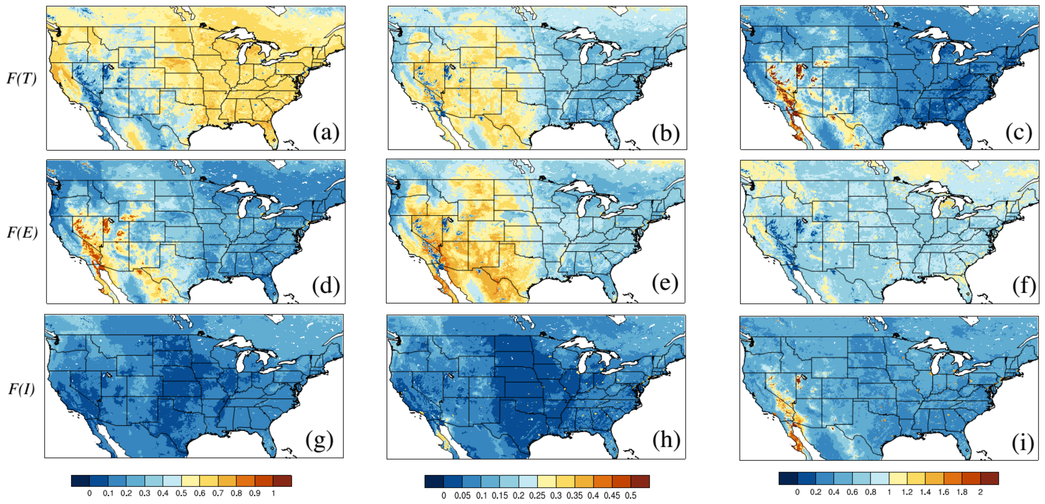
The mean, standard deviation and CV of $F(T)$, $F(E)$ and $F(I)$ derived from Equation (2) across the models are shown in Figure 3. There is significant spatial variability in the $F(T)$ and $F(E)$ estimates, whereas the models show much less variation in $F(I)$, which is generally below 20% of the total $ET$. Transpiration is the dominant source of $ET$ over the vegetation dominated Eastern U.S., whereas soil evaporation is the dominant source only in the more arid parts of Western U.S. The multi-model standard deviation of $F(T)$ and $F(E)$ is low in the Eastern U.S. and high in the Western U.S., indicating that the models agree in the fractional partition over the Eastern U.S. and disagree over the Western U.S., which is different from the pattern of larger standard deviation in total $ET$ over the Eastern U.S. The GVF/LAI values used in these LSMs are higher in the Eastern U.S., leading the models to consistently have a higher $F(T)$. However, the exact magnitude of T and thus total $ET$ in the East varies between LSMs due to their individual parameterizations of calculating the canopy resistance. In other words, the models are very similar in the Eastern U.S. in partitioning total $ET$ into T or I due to high GVF/LAI values, but differ in calculating the magnitudes. In the Western U.S., the magnitudes of $ET$ are lower due to lower soil moisture as well as lower GVF/LAI values. Here, the LSMs vary in partitioning between T and E as a result of differences in calculating soil evaporation discussed in Section 2 (e.g., VIC not considering soil evaporation underlying vegetation, Noah-MP’s dynamic vegetation potentially simulating different vegetation amounts than the other LSMs, CLSM’s three regions of soil moisture heterogeneity). In the West, the LSMs tend to more consistently simulate lower ET, but differ in how this $ET$ is partitioned. This result is consistent with the similarity analysis of $ET$ presented in [27]. Similarly, the CV values of $F(T)$ is higher in the West and lower in the East, unlike the pattern of CV for the total $ET$. The relative variability of $F(E)$ and $F(I)$, on the other hand, is more uniform across the domain. It is worth noting that, relative to $ET$ model intercomparison efforts, only a few studies have examined the inter-model differences in the $ET$ partition components. When comparing three process-based $ET$ estimates, Ref. [7] reports similar spatial patterns of T and E and I over the CONUS.

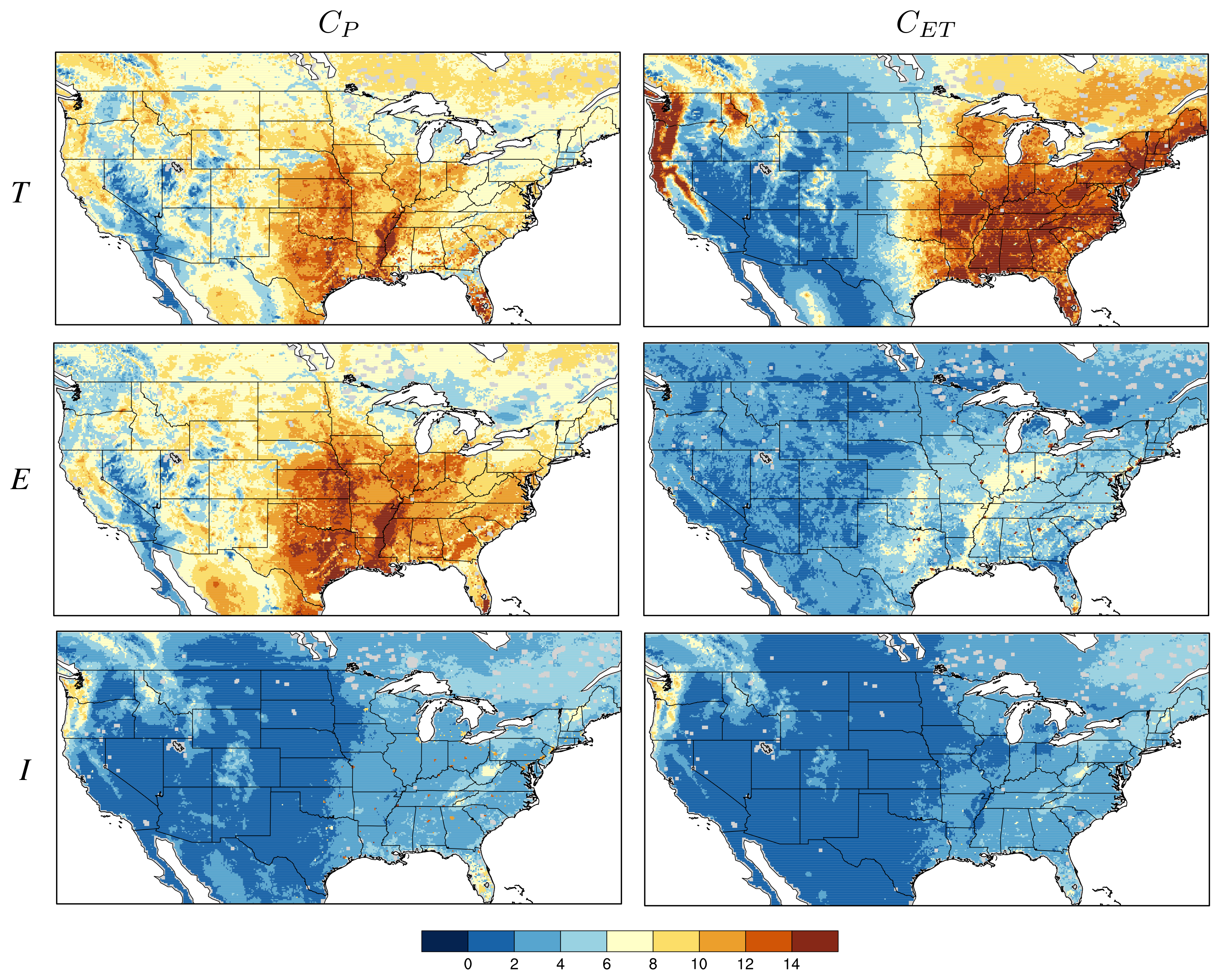
Figure 3 indicates that the fractional partitioning ($F(S)$) alone does not explain the aggregate differences in the domain-wide $ET$ partitioning seen in Figure 1, only in combination with the magnitude of total $ET$ can the real cause of these inter-model variations be understood. The contribution of these two sources of uncertainty in domain-wide $ET$ partitioning, the uncertainty in local partitioning and the uncertainty in total $ET$ are quantified by $C_P$ and $C_{ET}$ estimates’ Equations (3) and (4) and are shown in Figure 4. For T and E, the contribution of the partition uncertainty is high in the Eastern U.S. and lower in the Western U.S. Note that this behavior is different from the patterns in Figure 3, where the standard deviation of the T and E fractions is higher in the West and lower in the East. In other words, the uncertainty in local $ET$ partition shows different trends when they are scaled by the multimodel average $ET$. Similarly, the $C_{ET}$ maps show larger values in the east and lower estimates in the west, particularly for T. In the $C_P$ maps, the magnitudes for T and E are comparable, whereas the T uncertainty is significantly higher than that of E in the $C_{ET}$ comparisons. This implies that, whereas the contribution of the partition uncertainty is comparable for T and E, the contribution of uncertainty in total $ET$ has a more dominant effect for T. Again, the LSMs differ in how they calculate the canopy resistance, leading to larger variability in the magnitude of T in areas with higher total $ET$ and GVF/LAI. A similar east–west contrast in the uncertainty contributions is seen in the $C_P$ and $C_{ET}$ maps for I, though the magnitudes of the uncertainty contributions are smaller than that of T and E. The patterns in the Figure 3 and Figure 4 also indicate the strong influence of water availability, a factor that is known to be a key driver of $ET$ uncertainty ([42]).

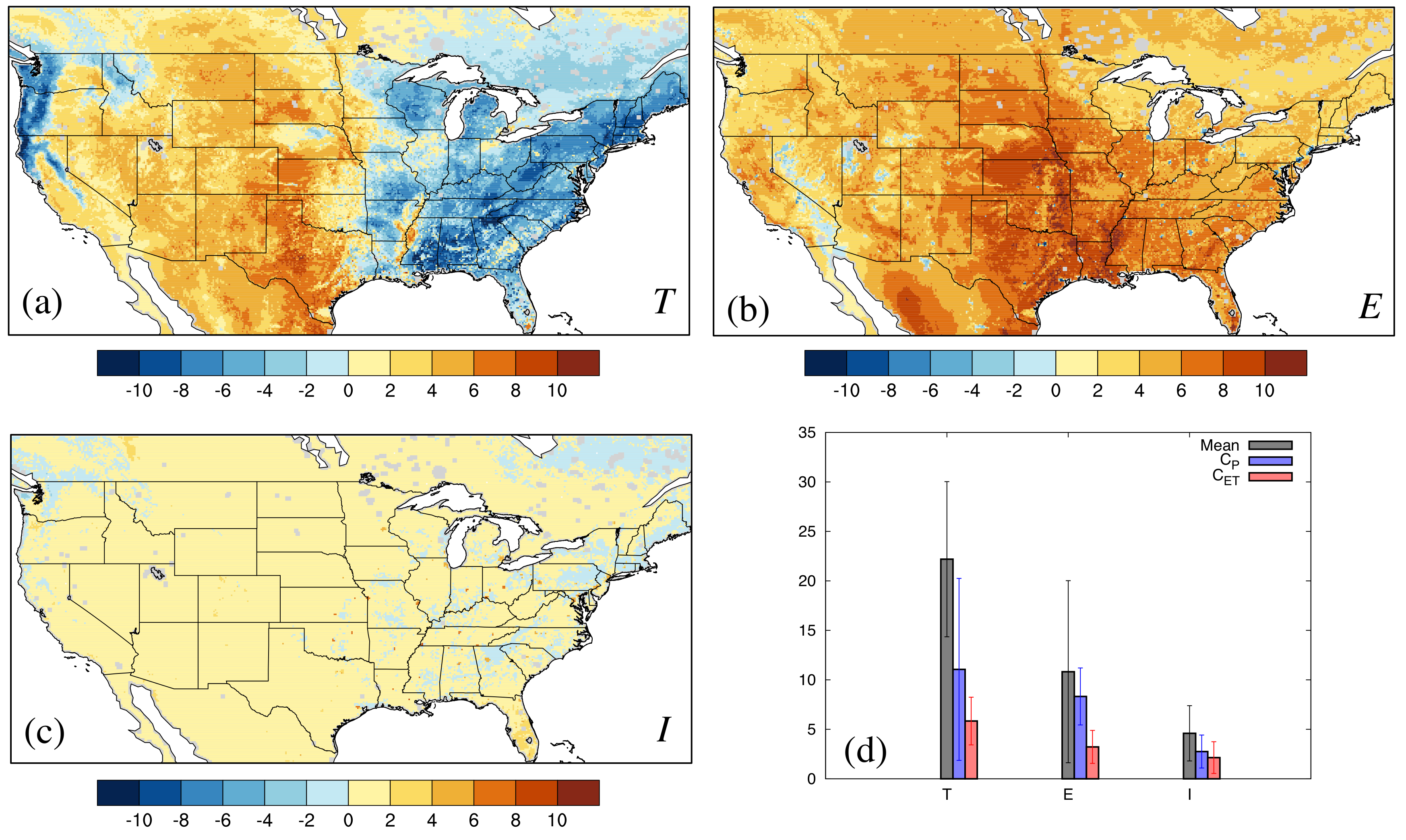
Comparison of $C_P$ and $C_{ET}$ estimates can be used to develop attributions of uncertainty for each component in each region. Figure 5 shows the maps of differences in the contribution terms of $C_P$ and $C_{ET}$. It can be seen that the contribution of uncertainty in total ET dominates the inter-model spread in $ET$ partition of T over the Eastern U.S., whereas the contribution of the partitioning uncertainty is more dominant in other regions. For E, the $C_P$ is the dominant source of uncertainty throughout the domain. The relative contributions of the two sources of uncertainty are small and spatially uniform for I. The largest uncertainties in $C_P$ and $C_{ET}$ are seen over the south-central U.S. Spatially, the fraction of $C_P$ and $C_{ET}$ varies between approximately 10 to 30% for both T and E, suggesting that the contributions of these uncertainty factors are non-trivial over majority of the domain. Panel (d) of Figure 5 presents the domain averaged values of the $ET$ components, the $C_P$ and $C_{ET}$ factors and their respective standard deviations, which quantifies that the partitioning uncertainty in the models is the major contributor to the inter-model differences in the constituent $ET$ partition terms.

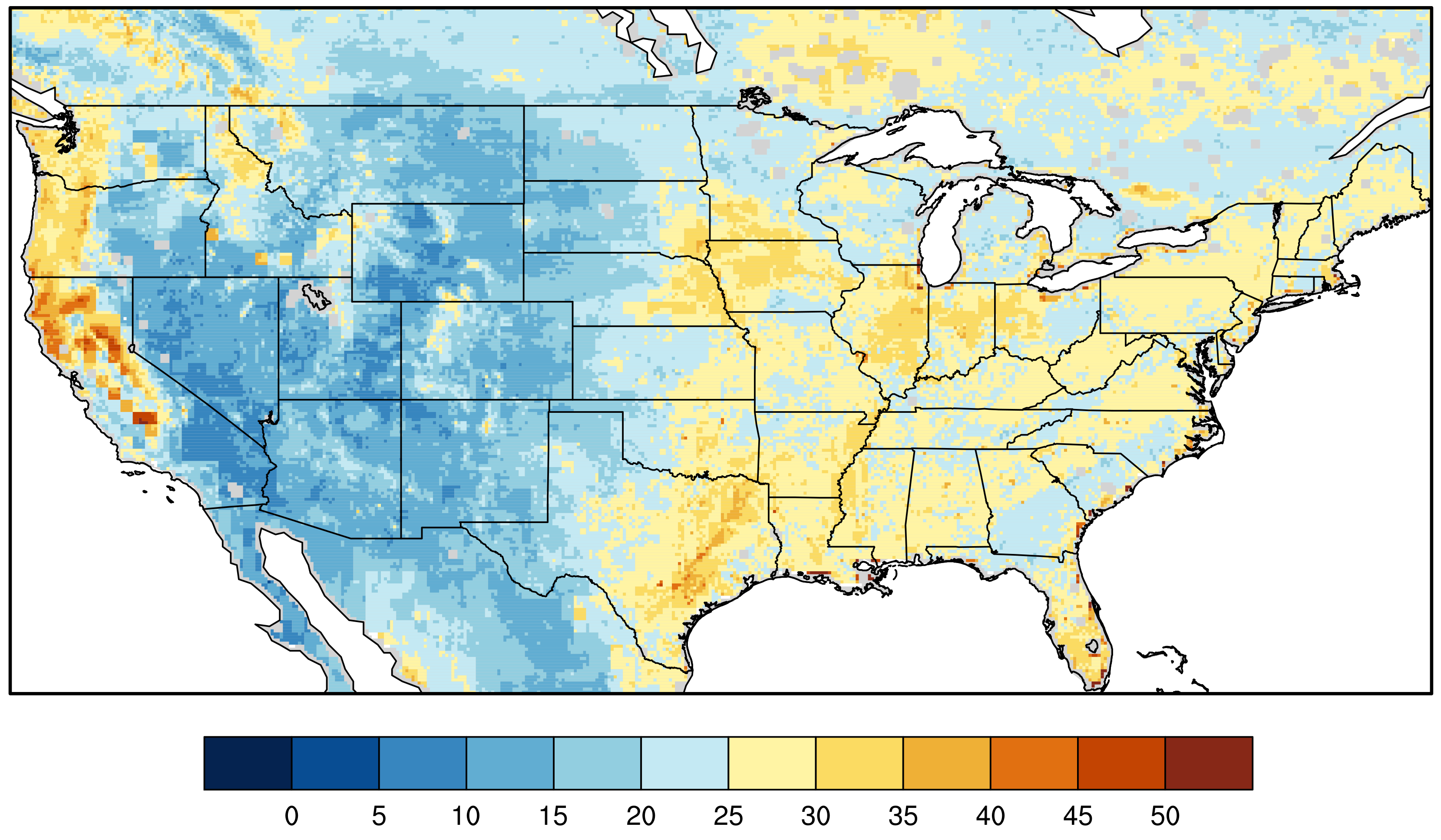
Figure 5 is helpful in determining the major factors of uncertainty in the $ET$ partitioning at a particular location and evaporation source. We also examine how these component uncertainties impact the accuracy of the $ET$ estimates. Mean $ET$ root mean square difference (RMSD) of the LSMs is estimated by comparing to the gridded FLUXNET multi tree ensemble (MTE) ([43]) data and is shown in Figure 6. The FLUXNET MTE data is a synthesis product that combines the information from station flux and meteorological measurement to produce a spatially distributed product at monthly time scale. The average RMSD in $ET$ is higher in the East and lower in the West, which mirrors the pattern of east–west contrast of $(C_P(T)-C_{ET}(T))$ (and the pattern of standard deviation of total $ET$ in Figure 2). The average RMSD in $ET$ is highest in areas where the mean $ET$ is high (Figure 2a); areas that also have T as the dominant source of $ET$ (Figure 3a). This means that, for use of $ET$ estimates in CONUS-wide water balance applications (where absolute values are important), transpiration stands out as the key process to improve, and that uncertainty in total $ET$ is the largest contribution to errors in T (Figure 5a).

The relative contribution of the partitioning uncertainty and total $ET$ was also examined by stratifying by season (Figure 7). The strong influence of warm seasonality is obvious in these comparisons, consistent with the literature on $ET$ uncertainty ([42]). Similar patterns to that of Figure 4 and Figure 5, where $C_P$ is a dominant factor in the E partition and $C_{ET}$ as the dominant factor over the Eastern U.S. for T are observed in the seasonal stratifications. These patterns are most magnified over the summer (JJA), followed by the spring (MAM) and fall (SON) time periods. The contrast and the magnitude of uncertainty contribution factors were small during the winter time period (DJF). The dependence of the results on the choice of the models in the ensemble was also investigated using a reduced set of models, by excluding Noah-3.6 and VIC-4.1.2.l. The results were very similar, confirming that the conclusions presented here are not biased due to the use of some models (Noah-2.8 and Noah-3.6; VIC-4.0.3 and VIC-4.1.2.l) that are similar in their structure and parameterizations.

5. Conclusions

Evapotranspiration, representing the energy and moisture exchange between the land surface and the atmosphere is a critical term in the terrestrial water balance. $ET$ consists of three main components of transpiration, soil evaporation and canopy interception, which represent the primary physiological and biological controls on the carbon and water cycles. Understanding the variability of these constituent terms is necessary for improving the estimation of $ET$. Though LSMs provide an effective way to generate spatially and temporally continuous estimates of $ET$ and its components, several studies have reported large differences in the LSM-based $ET$ partitioning. Such uncertainties also impact the efficiency of data assimilation environments, which employ these LSMs for incorporating relevant remote sensing information to develop physically consistent representations of $ET$ and its components. This study explores the factors explaining such disagreements for the CONUS region using the outputs from a suite of LSMs in the NLDAS-2 project.

These models show large disagreements in the average T and E fractions as well as the total $ET$ over the CONUS domain. The transpiration component dominates the $ET$ partition in the multimodel average, accounting for 53.6% of the total $ET$. The soil evaporation and canopy interception accounts for 30.8% and 15.6% of the total $ET$. The spatial distribution of the $ET$ partition shows significant variability with the T and E dominating the $ET$ partition over the Eastern and Western U.S., respectively. Since the magnitude of the total $ET$ is a significant factor in the inter-model differences in T and E, the article presents an approach to isolate the contribution of the partitioning uncertainty ($C_P$) and the uncertainty in total $ET$ ($C_{ET}$) to the $ET$ partitioning. $C_P$ is estimated by scaling the multimodel average $ET$ with the standard deviation of the fraction of the evaporation balance, whereas $C_{ET}$ is estimated by scaling the average fraction of the evaporation balance with the standard deviation in the total $ET$. The regional breakdown of uncertainty in the $ET$ partition shows that the contribution of uncertainty in total $ET$ to the T uncertainty is dominant over the Eastern U.S., whereas the uncertainty from partitioning is the dominant factor over the Western U.S. The results also indicate that the sources of uncertainty in T are key contributors of overall errors in total $ET$. For E, $C_P$ is the major factor of uncertainty throughout the domain. These trends persist in the seasonal stratification with the largest uncertainties in summer (JJA), followed by spring (MAM), fall (SON) and winter (DJF) time periods.

The analysis in the article suggests that model formulation and parameterization differences are key sources of uncertainty in the $ET$ partitioning. The areas with relatively high agreements in the $ET$ partition and total $ET$ are limited to areas in the west with moderate vegetation. Compared to the total $ET$, over most regions of the CONUS, the fraction of $C_P$ and $C_{ET}$ for T and E to the total $ET$ ranges approximately from 10 to 30%, indicating that the contribution of these factors to the overall $ET$ inter-model spread is significant. This study also suggests that efforts to reduce the $ET$ partition uncertainties in the model are needed to reduce the inter-model differences in E and T estimates from the LSMs. Improving upon the simple representations of parameters such as vegetation fraction, vegetation/radiative stress functions and rooting depth that are currently employed by the LSMs is likely needed for improving the skill and reducing the uncertainty of the $ET$ terms. Similarly, improving the model formulations of I would be beneficial in reducing the uncertainty in $ET$, particularly over vegetated areas. Recent studies such as [44] have also highlighted the significant sensitivity of flux estimates from the LSMs to model parameters and the need to calibrate and improve them. Over transpiration-dominated areas (e.g., Eastern U.S.), efforts to reduce the uncertainty in partitioning of the available net radiation is also needed for improving the level of agreement between models.