Article

Evolution of the Performances of Radar Altimetry Missions from ERS-2 to Sentinel-3A over the Inner Niger Delta

1
Oceanic and Continental Environments and Paleoenvironments (EPOC), Mixed Research Unit (UMR) 5805, University of Bordeaux, Allée Geoffroy Saint-Hilaire, 33615 Pessac, France
2
Geosciences Environment Toulouse (GET), University of Toulouse, National Center for Scientific Reaseach (CNRS), Institute for Research and Development (IRD), UPS. Observatory Midi-Pyrénées (OMP), 14 Av. E. Belin, 31400 Toulouse, France
3
Laboratory of Studies on Spatial Geophysics and Space Oceanography (LEGOS), University of Toulouse, National Center for Space Studies (CNES), CNRS, IRD, UPS. OMP, 14 Av. E. Belin, 31400 Toulouse, France
4
Department of Education and Research (DER) Math-Informatics, Faculty of Sciences and Technology (FST)/University of Sciences, Techniques and Technologies of Bomako (USTTB), Bamako 3206, Mali
5
National Research Institute of Science and Technology for Environment and Agriculture (IRSTEA), IRD, 361 rue Jean-François Breton, 34196 Montpellier, France
6
Laboratory of Optics, Spectroscopy and Atmospheric Sciences (LOSSA), Department of Education and Research (DER) Physics, Faculty of Sciences and Technology (FST)/University of Sciences, Techniques and Technologies of Bomako (USTTB), Bamako 3206, Mali
*
Author to whom correspondence should be addressed.
Submission received: 14 March 2018 / Revised: 16 May 2018 / Accepted: 23 May 2018 / Published: 25 May 2018
(This article belongs to the Special Issue Satellite Altimetry for Earth Sciences)

Abstract

:
Radar altimetry provides unique information on water stages of inland hydro-systems. In this study, the performance of seven altimetry missions, among the most commonly used in land hydrology (i.e., European Remote-Sensing Satellite-2 (ERS-2), ENVIronment SATellite (ENVISAT), Satellite with Argos and ALtika (SARAL), Jason-1, Jason-2, Jason-3 and Sentinel-3A), are assessed using records from a dense in situ network composed of 19 gauge stations in the Inner Niger Delta (IND) from 1995 to 2017. Results show an overall very good agreement between altimetry-based and in situ water levels with correlation coefficient (R) greater than 0.8 in 80% of the cases and Root Mean Square Error (RMSE) lower than 0.4 m in 48% of cases. Better agreement is found for the recently launched missions such as SARAL, Jason-3 and Sentinel-3A than for former missions, indicating the advance of the use of the Ka-band for SARAL and of the Synthetic-aperture Radar (SAR) mode for Sentinel-3A. Cross-correlation analysis performed between water levels from the same altimetry mission leads to time-lags between the upstream and the downstream part of the Inner Niger Delta of around two months that can be related to the time residence of water in the drainage area.

Graphical Abstract

1. Introduction

Surface waters, which are part of the continental branch of the terrestrial water cycle, play an essential role in supplying fresh water for basic human and economic needs. They are strongly impacted by climate changes and anthropogenic pressures caused by population growth and changes in agricultural practices [1,2,3]. Despite the importance of their monitoring for addressing integrated water resource management, use in operational flood forecasting or disaster mitigation, reliable in situ measurements of water stage and discharge has become increasingly scarce information due to either the disappearance of the gauge networks or the difficulty to get access to data [4,5].
Satellite radar altimetry, initially developed for the measurement of the ocean surface topography through the measurement of the distance between the Earth’s surface and the spaceborne radar altimeter [6], has demonstrated its efficiency for deriving water levels of inland water bodies (see Crétaux et al. [7] for a recent review). Radar altimetry, was initially used over land to retrieve water levels over homogeneous surfaces such as large lakes and enclosed seas [8,9], but also at cross-sections between rivers and altimetry ground-tracks of several kilometers of width in large river basins [10,11]. These early results were obtained using Geosat and Topex/Poseidon (T/P) ranges (i.e., the distance between the satellite and the surface) derived from the Ocean retracking algorithm. Root Mean Square Errors (RMSE) lower than 0.05 m and 1.1 m through comparisons with in situ water stages were obtained over lakes and rivers respectively. The comparisons are performed at the so-called Virtual Stations. Virtual stations (VS) are defined as the cross-sections of an altimetry ground-track and a water body (i.e., lake, reservoir river channel, floodplain, or wetland) where the temporal variations of the height from one cycle to the next can be associated with changes in water level [7]. With the launch of ENVISAT in 2002, ranges processed using other retracking algorithms were included in the Geophysical Data Records (GDR) made available by space agencies. Among them, the Offset Center Of Gravity (OCOG, also known as Ice-1) was found to provide, most of the time, the most accurate estimate of river water levels (with RMSE generally lower than 0.3 m and correlation coefficient R greater than 0.9) [12]. Combined with the availability of land-dedicated corrections of the ionosphere, wet troposphere delays and improvements in the data processing, this allowed the generalization of the use of radar altimetry for the monitoring of inland waters [7,13].
Thanks to these different improvements and the use of high-frequency data (10, 18, 20 or 40 Hz depending on the altimetry mission) instead of 1 Hz data (~7 km of sampling along the track) as over the open ocean water bodies of a few or below one hundred meters of width can now be monitored with very good accuracy (e.g., [14,15,16]). As radar altimetry data have global coverage and are freely available, they are now commonly used in a wide range of hydrological applications (see Crétaux et al. [7] for a recent review), and, even in support for the management of in situ networks [17]. Until now, no study provided a systematic assessment of the performance over rivers of different altimetry missions that were operating since the beginning of the high-precision altimetry era, which started with the launch of Topex/Poseidon (T/P) in 1992, contrary to that done over lakes [18,19].
The goal of this study is to evaluate the quality of altimetry-based water levels for all missions in repetitive orbits whose data contained in the GDR were processed using the OCOG retracking algorithm. For this purpose, comparisons between altimetry-based water stages and in situ measurements from a dense gauges network were performed in the Inner Niger Delta (IND).
Several studies already used altimetry-based water levels to better understand spatio-temporal dynamics of the flood in this region [20,21,22] and to estimate river discharges [23,24]. The IND was chosen as study area as it is densely covered with (i) in situ gauge stations whose records are available over the whole high-precision altimetry era and (ii) cross-sections between altimetry ground-tracks from different missions and rivers of various widths.
A dense network of VS was built in the IND, composed of 52, 63, 623 VS for European Remote-Sensing Satellite-2 (ERS-2), ENVIronment SATellite (ENVISAT), Satellite with Argos and ALtika (SARAL) respectively, 31 for Sentinel-3A and 8, 8, 9 for Jason-1, Jason-2 and Jason-3 respectively. At each virtual station, time variations of river levels from radar altimetry are constructed.
In this study, comparisons between altimetry-based water stages derived from acquisitions of Jason-1, Jason-2 and Jason-3, ERS-2, ENVISAT, SARAL and Sentinel-3A and in situ water levels from 19 gauge stations located in the IND are presented in terms of RMSE and R. Intra-mission results consistency were also assessed through cross-correlations between virtual stations along the river.

2. Method

2.1. Principle of Radar Altimetry and Data Processing

2.1.1. Principle of Altimetry Measurement

The principle of radar altimetry is the following: a radar altimeter emits an electromagnetic wave in the nadir direction and measures its round-trip time. The distance between the satellite and the Earth surface—the altimeter range (R0)—is derived with a precision of a few centimeters. The satellite altitude (H) referred to an ellipsoid is determined from precise orbitography technique with accuracy better than 2 cm. Taking into account propagation corrections caused by delays resulting from interactions of electromagnetic wave with the atmosphere, and geophysical corrections, the height of the reflecting surface (h) with reference to an ellipsoid can be estimated as [25,26]:
h = H ( R 0 + ( Δ R p r o p a g a t i o n + Δ R g e o p h y s i c a l ) )
where H is the height of the center of mass of the satellite above the ellipsoid estimated using precise orbit determination (POD) technique, R0 is the nadir altimeter range from the center of mass of the satellite to the sea surface taking into account instrumental corrections.
Δ R p r o p a g a t i o n = Δ R i o n + Δ R d r y + Δ R w e t
where ΔRion is the atmospheric refraction range correction due to the free electron content associated with the dielectric properties of the ionosphere, ΔRdry is the atmospheric refraction range correction due to the dry gas component of the troposphere, ΔRwet is the atmospheric refraction range correction due to the water vapor and the cloud liquid water content of the troposphere.
Δ R g e o p h y s i c a l = Δ R s o l i d   E a r t h + Δ R p o l e
where ΔRsolid Earth and ΔRpole are the corrections respectively accounting for crustal vertical motions due to the solid Earth and pole tides.

2.1.2. Time Variations of River Levels from Radar Altimetry Measurements

In this study, the Multi-mission Altimetry Processing Software (MAPS), developed by Frappart et al. [27] was used to visualize and process the altimetry data over land [22,28,29,30] and ocean [31,32] to build the VS in the IND. Data processing is composed of three main steps: (i) a coarse delineation of the VS using Google Earth; (ii) a refined selection of the valid altimetry data based on visual inspection; and (iii) the computation of the time series of water level. The altimetry-based water level is computed for each cycle using the median of the selected altimetry heights, along with their respective deviation (i.e., mean absolute deviation). This process is repeated each cycle to construct the water level time series at the virtual stations and illustrated in Figure 1.
Altimetry datasets are referenced either to WGS84 ellipsoid or to Topex/Poseidon ellipsoid. A datum conversion from T/P ellipsoid to WGS84 is automatically performed using Equation (4) adapted from Jekeli et al. [33] and implemented in the version of MAPS used in Salameh et al. [34]:
Δ h = a ( 1 e 2 ) 1 e 2 sin 2 φ a ( 1 e 2 ) 1 e 2 sin 2 φ
where ∆h is the variation of height at latitude φ due to the change of ellipsoid from T/P to WGS84 datum, a = 6, 378, 137 m and e = 0.081819190842621 are the semi-major axis and the eccentricity of the WGS84 datum, a’ = 6,378,136.3 m and e’ = 0.081819221456 are the semi-major axis and the eccentricity of the T/P datum.
Some along-track altimetry profiles exhibit a parabolic shape caused by non-nadir reflections known as hooking effect (see Figure 2). Hooking effect is corrected as follows:
h ( s 0 ) = h ( s i ) + 1 2 R c o r r ( s 0 ) ( 1 + ( H s ( s i ) ) 2 ) d s 2
where s is the along-track coordinate, h(s0) is the altimeter height at nadir, Rcorr(s0) the altimeter range at nadir corrected from the geophysical and environmental effects, s0 the location of the nadir along the altimeter track, si the coordinates of the slant measurements, H / s the rate of altitude variation of the satellite along the orbital segment, and ds the along track difference between s0 and si. Then, the altimeter height at nadir is computed using the summit of the parabola representing the actual water level:
h ( s 0 ) = a s 0 2 + b s 0 + c
where a, b and c are parabola coefficients calculating using a least-square fitting of the altimeter data affected by hooking.
Finally, s0 and h(s0) are defined as follow:
s 0 = b 2 a   and   h ( s 0 ) = c b ² 4 a
h ( s 0 ) = a s 0 2 + b s 0 + c

2.2. Validation of the Altimetry-Based Water Levels

Validation of the altimetry-based water levels is performed against records from the closest in situ gauge stations. The along-stream distance between a VS and the closest in situ gauge stations is generally lower than 100 km (see Tables S1–S5). Root Mean Square Error (RMSE), R and R2 values were estimated between altimetry-based water levels and in situ ones measured the same day using the classical formulas:
RMSE = ( 1 n i = 1 n ( h a l t i ( t i ) h i n   s i t u ( t i ) ) 2 ) 1 / 2
R = i = 1 n ( h a l t i ( t i ) h a l t i ( t i ) ) ( h i n   s i t u ( t i ) h i n   s i t u ( t i ) ) ( i = 1 n ( h a l t i ( t i ) h a l t i ( t i ) ) 2 ) 1 / 2 ( i = 1 n ( h i n   s i t u ( t i ) h i n   s i t u ( t i ) ) 2 ) 1 / 2
R 2 = i = 1 n ( h a l t i ( t i ) h i n   s i t u ( t i ) ) 2 i = 1 n ( h i n   s i t u ( t i ) h i n   s i t u ( t i ) ) 2
where halti and hin situ are the altimetry-based and the in situ water stages respectively, ti is the measurement time and n the number of common observations. The average of a variable x is written <x>.
As the in situ gauge stations are leveled against a reference unavailable to us, no bias estimates were computed between the in situ and the altimetry-based water levels, but they were between the different missions in the same orbit as follows:
Bias = 1 n i = 1 n ( h a l t i 1 ( t i ) h a l t i 2 ( t i ) )
while halti1 is the more recent mission in the orbit and halti2 is the older one.
The consistency of the intra-mission altimetry-based water levels as well as likely time-lag between water stages in the IND were estimated using the maximum of the cross-correlation function Rhh and the argument of the maximum:
R hh ( τ ) = i = 1 n ( h a l t i ( t i ) h a l t i ( t i ) ) ( h i n   s i t u ( t i τ ) h i n   s i t u ( t i ) ) ( i = 1 n ( h a l t i ( t i ) h a l t i ( t i ) ) 2 ) 1 / 2 ( i = 1 n ( h i n   s i t u ( t i τ ) h i n   s i t u ( t i ) ) 2 ) 1 / 2
where τ is the time displacement.

3. Study Area and Datasets
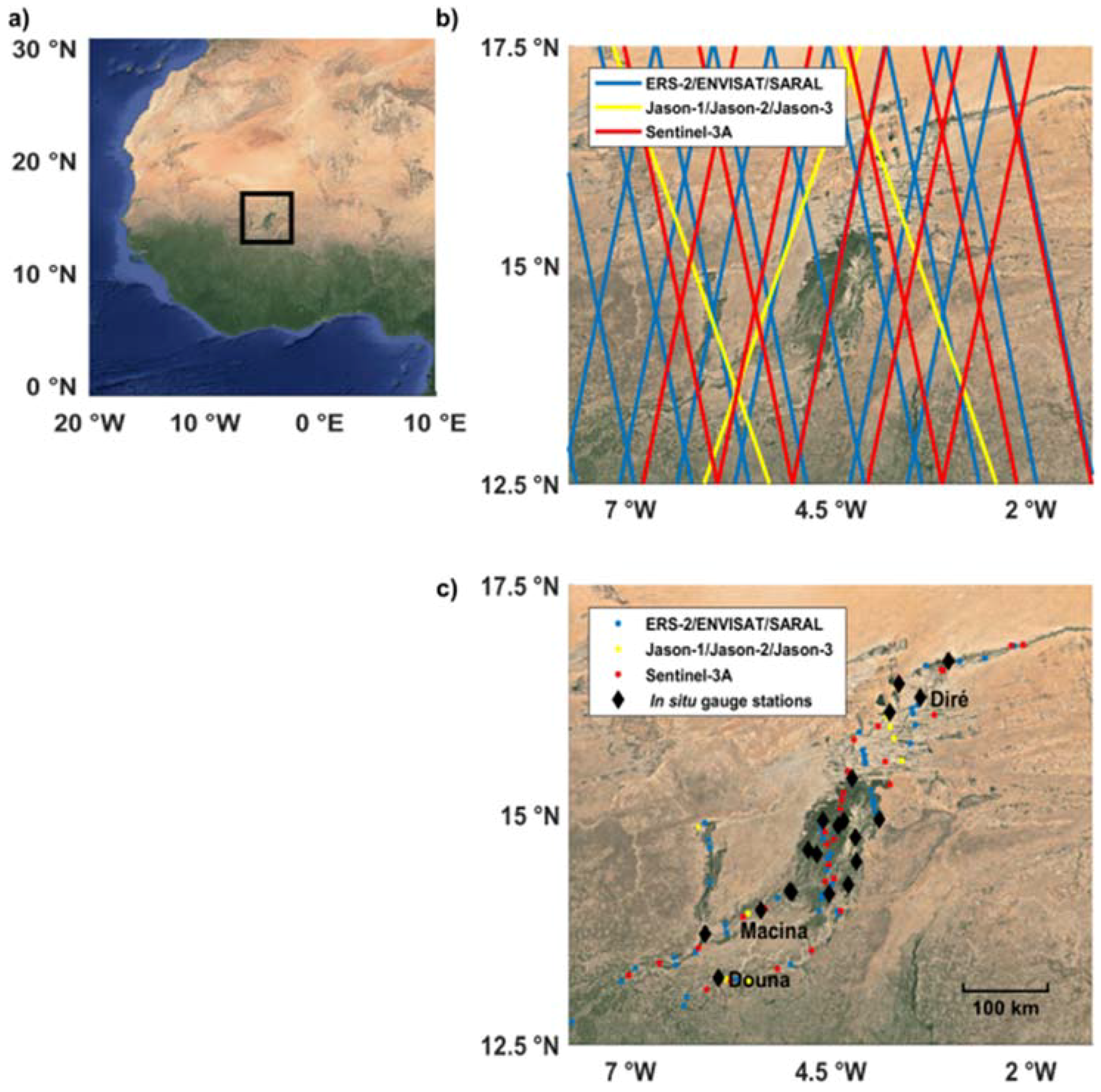
3.1. Study Area

The IND is an extensive Sahelian floodplain located between longitudes 3–5° W and latitudes 13–17° N in Central Mali (Figure 3a). It is encompassed between the in situ gauge stations of Macina (−5.37° W, 13.95° N), on the Niger River, and Douna (−5.9° W, 13.22 °N), on the Bani River, upstream, and Diré (−3.38° W, 16.27° N), downstream. Its drainage area represents a surface of 73,000 km2 [35]. The flooded area extent depends on the intensity of the West African Monsoon and can reach 35,000 km2 during the wettest rainy seasons [36,37,38,39,40]. The flooding period ranges from August to December and during the dry season, from March to May, the area dries out with the exception of the rivers mainstem and the permanent lakes3.2. Radar Altimetry Data
The data used in this study come from the acquisitions of the following radar altimetry missions in their nominal orbit: Jason-1 (2002–2008), Jason-2 (2008–2016), Jason-3 (since 01/2016), ERS-2 (05/1995–06/2003), ENVISAT (03/2002–10/2010), SARAL (02/2013–2016), Sentinel-3A (since 02/2016). The main characteristics of these missions are presented below.

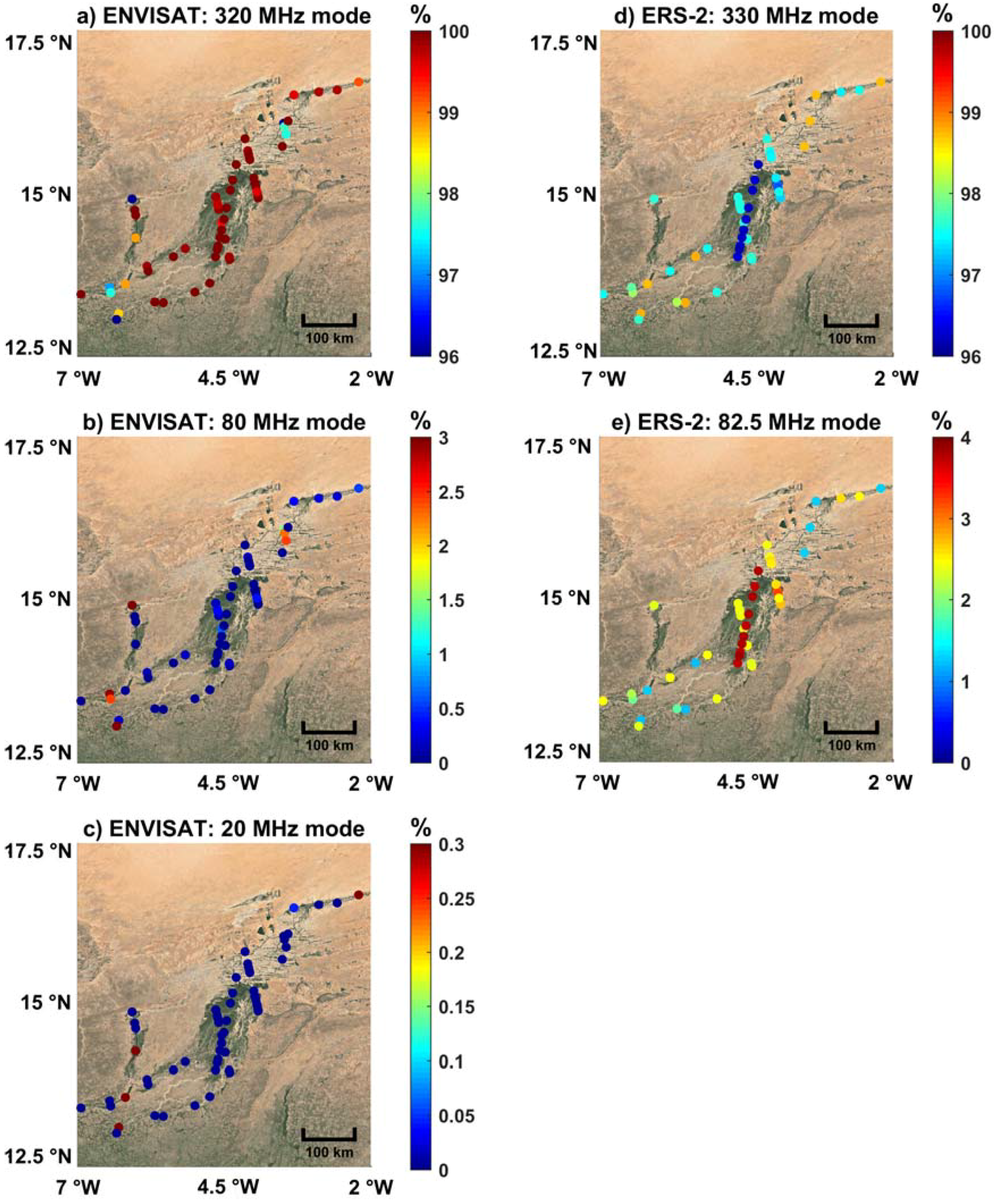
3.2.1. Missions with a 35-Day Repeat Period (European Remote-Sensing Satellite-2 (ERS-2), ENVIronment SATellite (ENVISAT), Satellite with Argos and ALtika (SARAL))

ERS-2, ENVISAT and SARAL orbited at an average altitude of 790 km, with an inclination of 98.54°, in a sun-synchronous orbit with a 35-day repeat cycle. They provided observations of the Earth surface (ocean, land, and ice caps) from 82.4° latitude north to 82.4° latitude south. This orbit was formerly used by ERS-1 mission, with an equatorial ground-track spacing of about 85 km.
ERS-2 was launched in 1995 by the European Space Agency (ESA) as ERS-1 follow-on mission. The satellite carries, among other instruments, a radar altimeter (RA) operating at Ku-band (13.8 GHz) developed for measuring height over ocean, land and ice caps. ERS-2 data are available from 17 May 1995 to 9 August 2010. After 22 June 2003, the dataset coverage is limited to ground station visibility.
ENVISAT mission was launched on 1 March 2002 by ESA. It carried 10 instruments including the advanced radar altimeter (RA-2). It was based on the heritage of the sensor on-board the ERS-1 and 2 satellites. RA-2 was a nadir-looking pulse-limited radar altimeter operating at two frequencies at Ku- (13.575 GHz), as ERS-1 and 2, and S-(3.2 GHz) bands [41]. ENVISAT remained in its nominal orbit until October 2010 and its mission ended on 8 April 2012. RA-2 stopped operating correctly at S-band in January 2008.
SARAL mission was launched on 25 February 2013. SARAL is a new collaboration between Centre National d’Etudes Spatiales (CNES) and Indian Space Research Organization (ISRO). Its payload comprises the AltiKa radar altimeter and bi-frequency radiometer, and a triple system for precise orbit determination: the real-time tracking system Détermination Immédiate d’Orbite par Doris embarqué (DIODE) of the Doppler Orbitography and Radio-positioning Integrated by Satellite (DORIS) instrument, a Laser Retroflector Array (LRA), and the Advance Research and Global Observation Satellite (ARGOS-3). AltiKa radar altimeter is a solid-state mono-frequency altimeter that provides accurate range measurements. It is the first altimeter to operate in the Ka-band (35.75 GHz) [42]. It has been put in a drifting orbit since July 2016.

3.2.2. Missions with a 10-Day Repeat Period (Jason-1, Jason-2 and Jason-3)

Jason-1, Jason-2 and Jason-3 orbit at an altitude of 1336 km, with an inclination of 66°, on a 10-day repeat cycle, providing observations of the Earth surface (ocean and land) from 66° latitude North to 66° latitude South, with an equatorial ground-track spacing of about 315 km. This orbit was formerly used by Topex/Poseidon mission.
Jason-1 mission was launched on 7 December 2001 by a cooperation between CNES and National Aeronautics and Space Administration (NASA). Jason-1 sensors are based on the former Topex/Poseidon missions, composed of the Poseidon-2 altimeter which is a two-frequency altimeter with C (5.3 GHz) and Ku (13.575 GHz) -bands. Its payload is also composed of the Jason Microwave Radiometer from NASA and a triple system for precise orbit determination: DORIS instrument from the CNES, Black Jack Global Positioning System receiver from NASA and a LRA from NASA/Jet Propulsion Laboratory (JPL) [43]. Jason-1 remained in its nominal orbit until 26 January 2009 and was decommissioned on 21 June 2013.
Jason-2 mission was launched on 20 June 2008 as a cooperation between CNES, the European Organization for the Exploitation of Meteorological Satellites (EUMETSAT), NASA and the National Oceanic and Atmospheric Administration (NOAA). Its payload is mostly composed of the Poseidon-3 radar altimeter from CNES, the Advanced Microwave Radiometer (AMR) from JPL/NASA, and a triple system for precise orbit determination: the real-time tracking system DIODE of DORIS instrument from CNES, a Global Navigation Satellite System (GNSS) receiver and a LRA from NASA/JPL. Poseidon-3 radar altimeter is a two-frequency solid-state altimeter that measures accurately the distance between the satellite and the surface (range) and provides ionospheric corrections over the ocean [44]. It operates at Ku and C bands. Raw data are processed by SSALTO (Segment Sol multimissions d’ALTimétrie, d’Orbitographie). Jason-2 remained in its nominal orbit until 3 July 2016.
Jason-3 mission was launched on 17 January 2016 as cooperation between CNES, EUMETSAT, NASA and NOAA. This satellite is composed of Poseidon-3B radar altimeter with a Precise Orbit Determination (POD) package with a Global Positioning System (GPS) receiver, DORIS and a LRA from NASA/JPL.

2.2.3. Mission with a 27-Day Repeat Period (Sentinel-3A)

Sentinel-3A mission was launched on 16 February 2016 by ESA to an orbit of altitude 814 km. The satellite caries one altimeter radar called SRAL (SAR Radar ALtimeter), a dual-frequency SAR altimeter (Ku-band at 13.575 GHz and C-band at 5.41 GHz). Its payload comprises also a Microwave Radiometer (MWR) instrument for wet path delay measurements and a triple system for precise orbit determination: a POD including a GPS receiver, a LRA and a DORIS instrument [45].
All this information is summarized in Table 1.
The data used in this study are summarized in Table 2. Ranges used to derive altimeter heights and backscattering coefficients are those processed with OCOG/Ice-1/Ice retracking algorithm [46]. Previous studies showed that Ice-1-derived altimetry heights are the more suitable for hydrological studies in terms of accuracy of water levels and availability of the data (e.g., [12,47,48]) among the commonly available retracked data present in the GDRs.

3.3. In Situ Water Levels
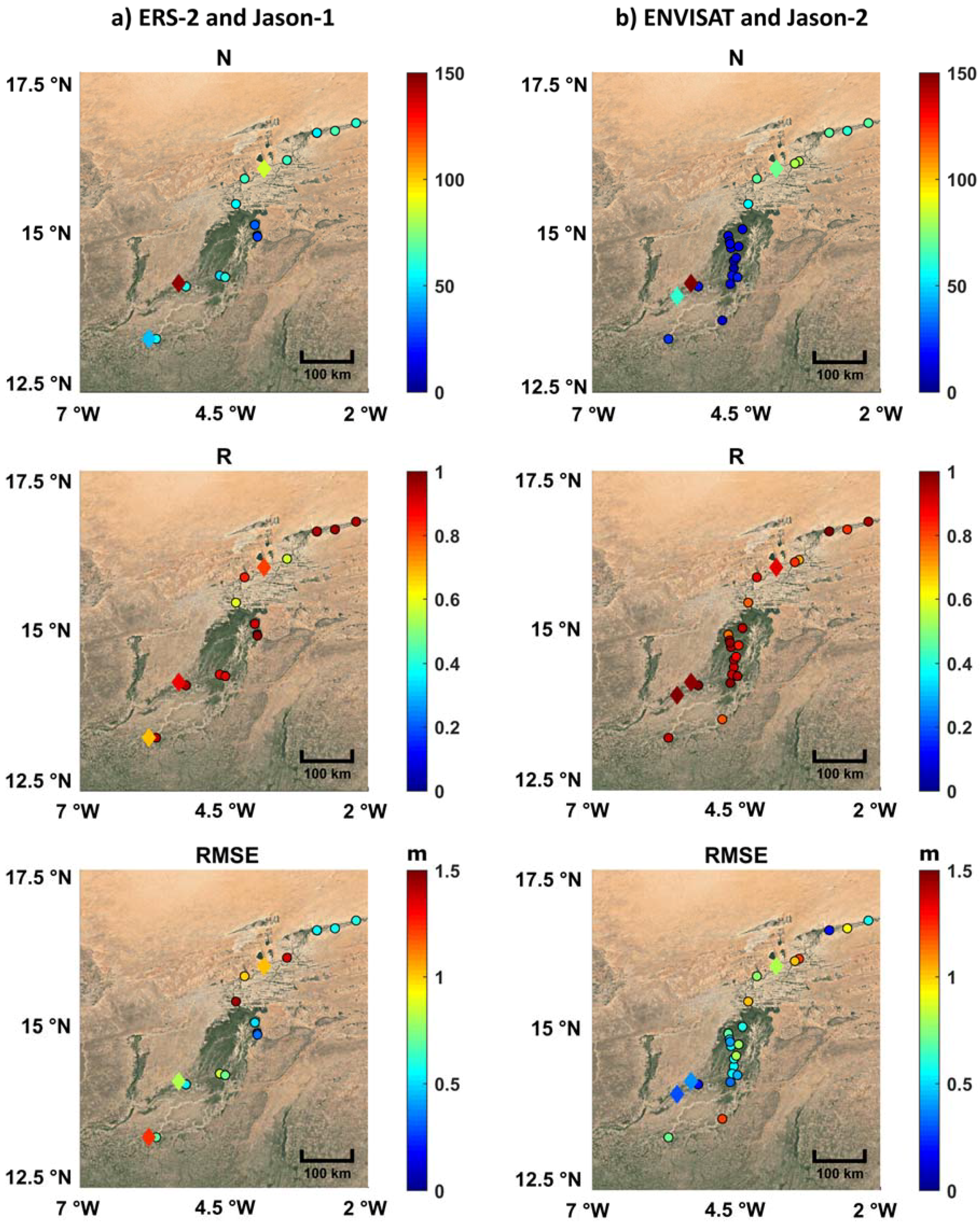
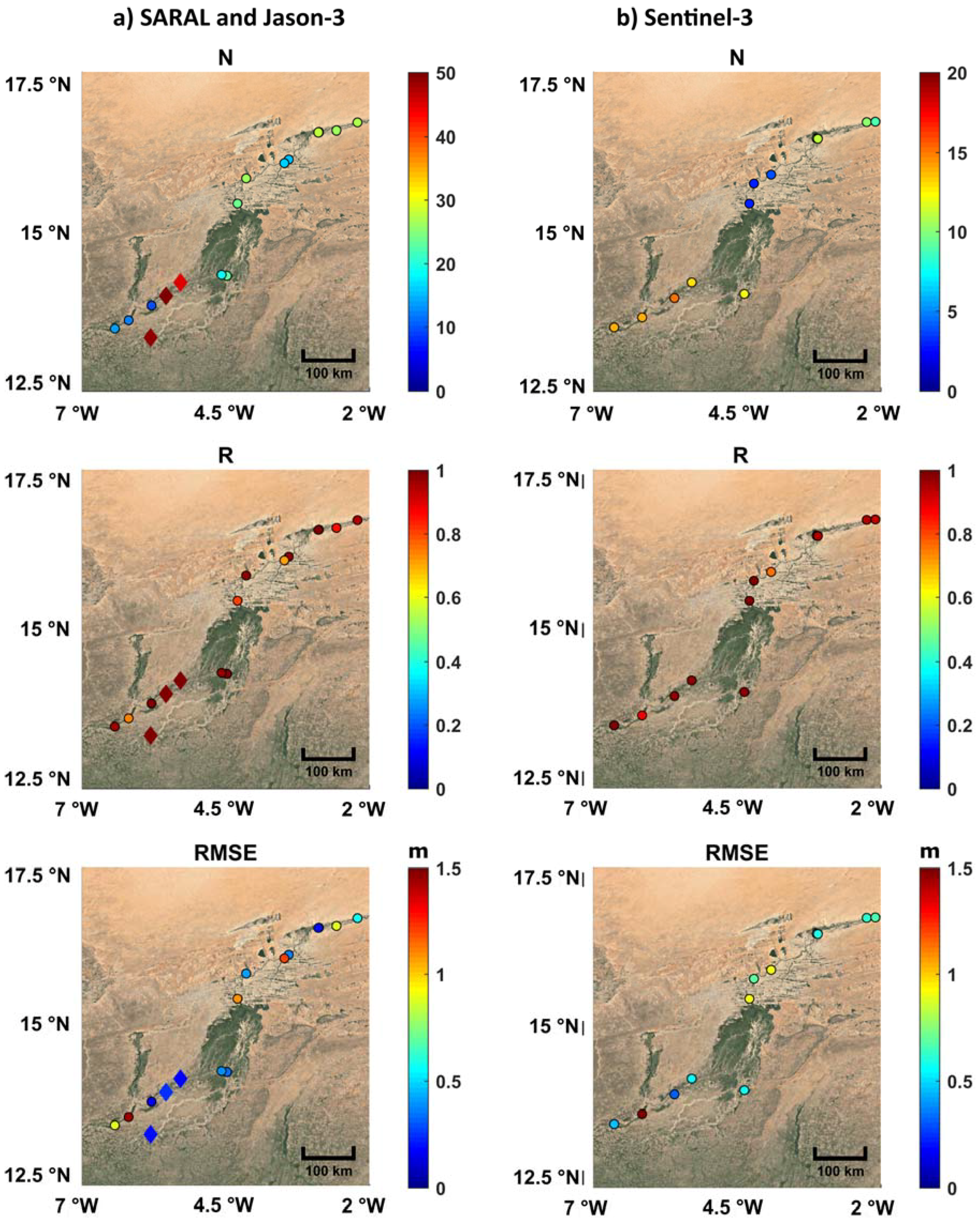
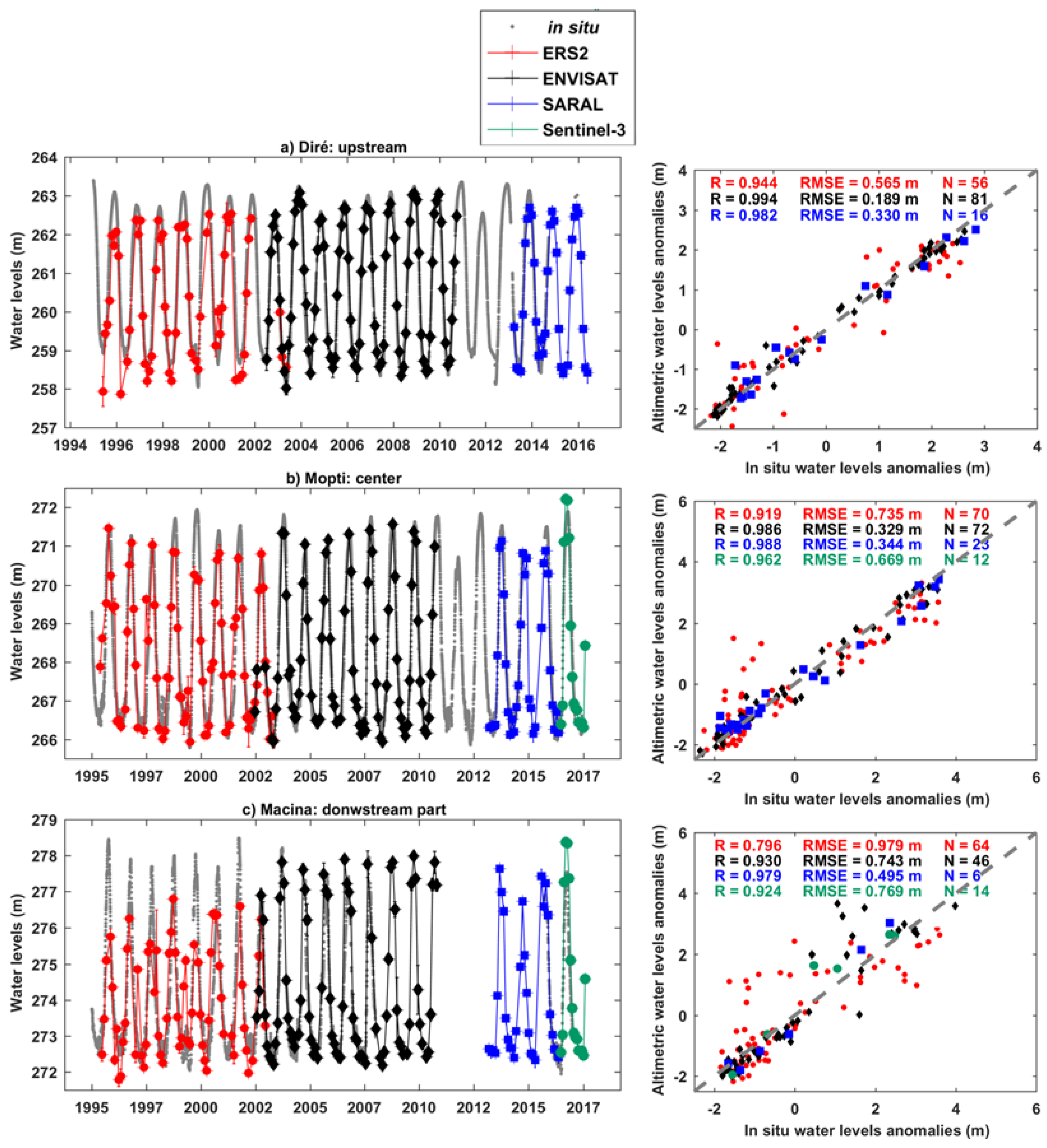
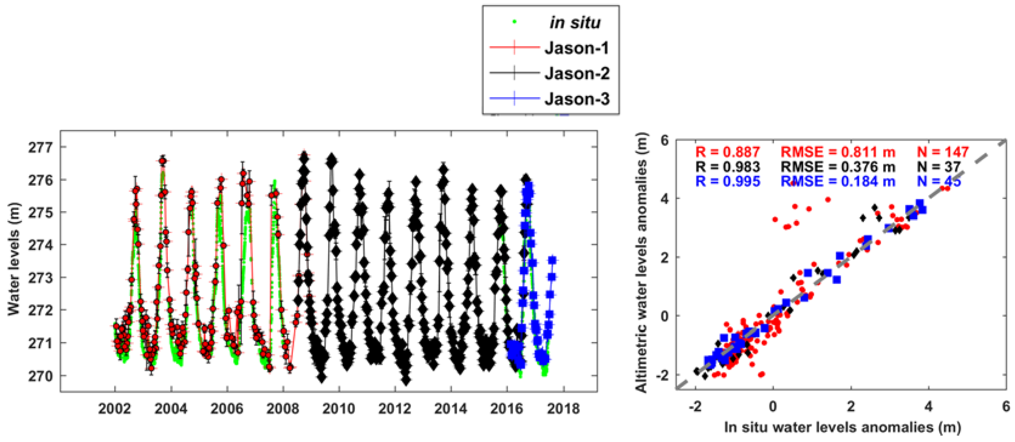
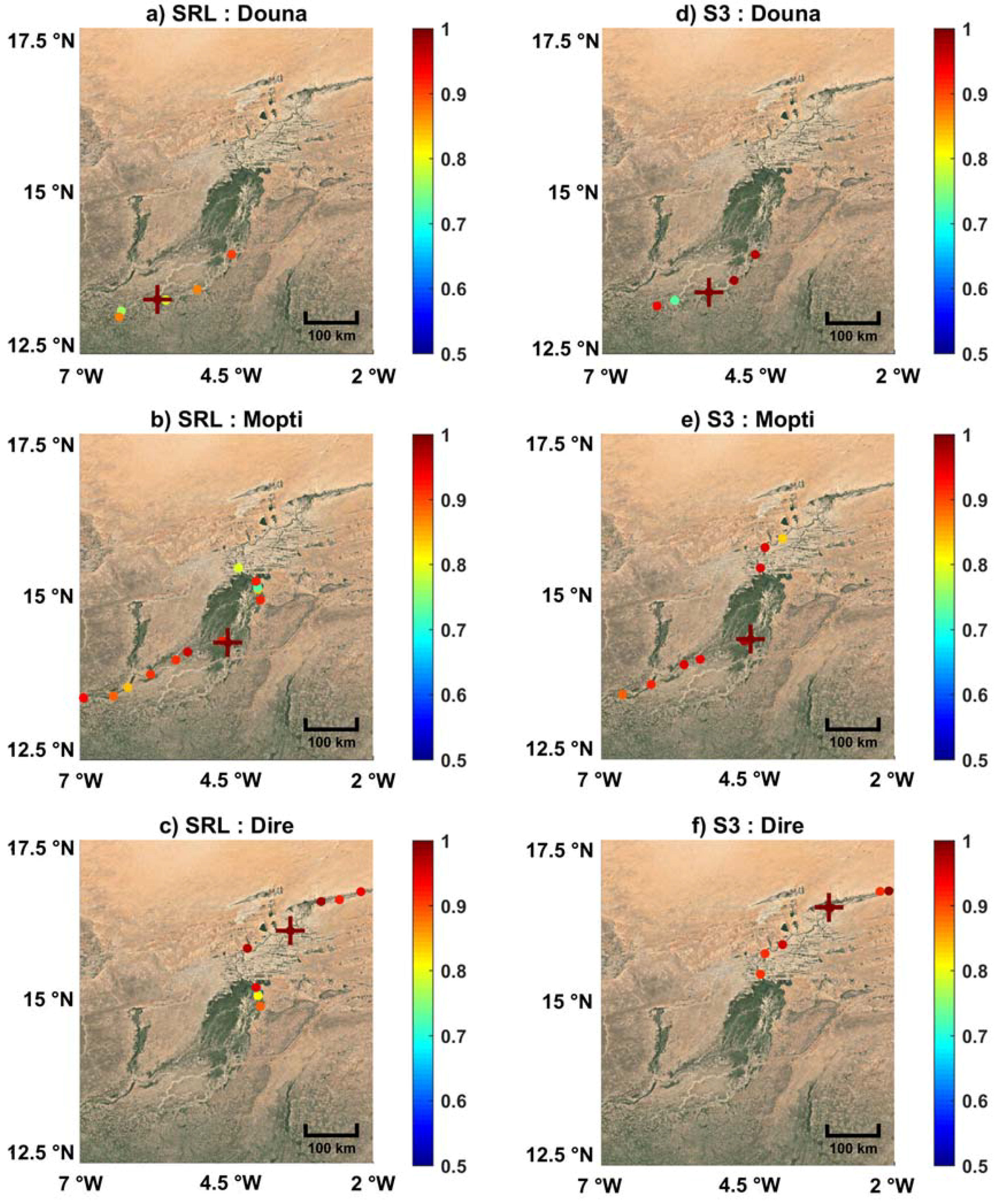
Daily stage records from 19 in situ gauge stations located in the IND were used in this study to validate altimetry-based water levels (see Table 3 for their names, locations and periods of data availability and Figure 3c for their locations). Measurements were acquired at 12:00 a.m. local time. They are made available by the Malian water agency (Direction Nationale de l’Hydraulique—DNH).

4. Results

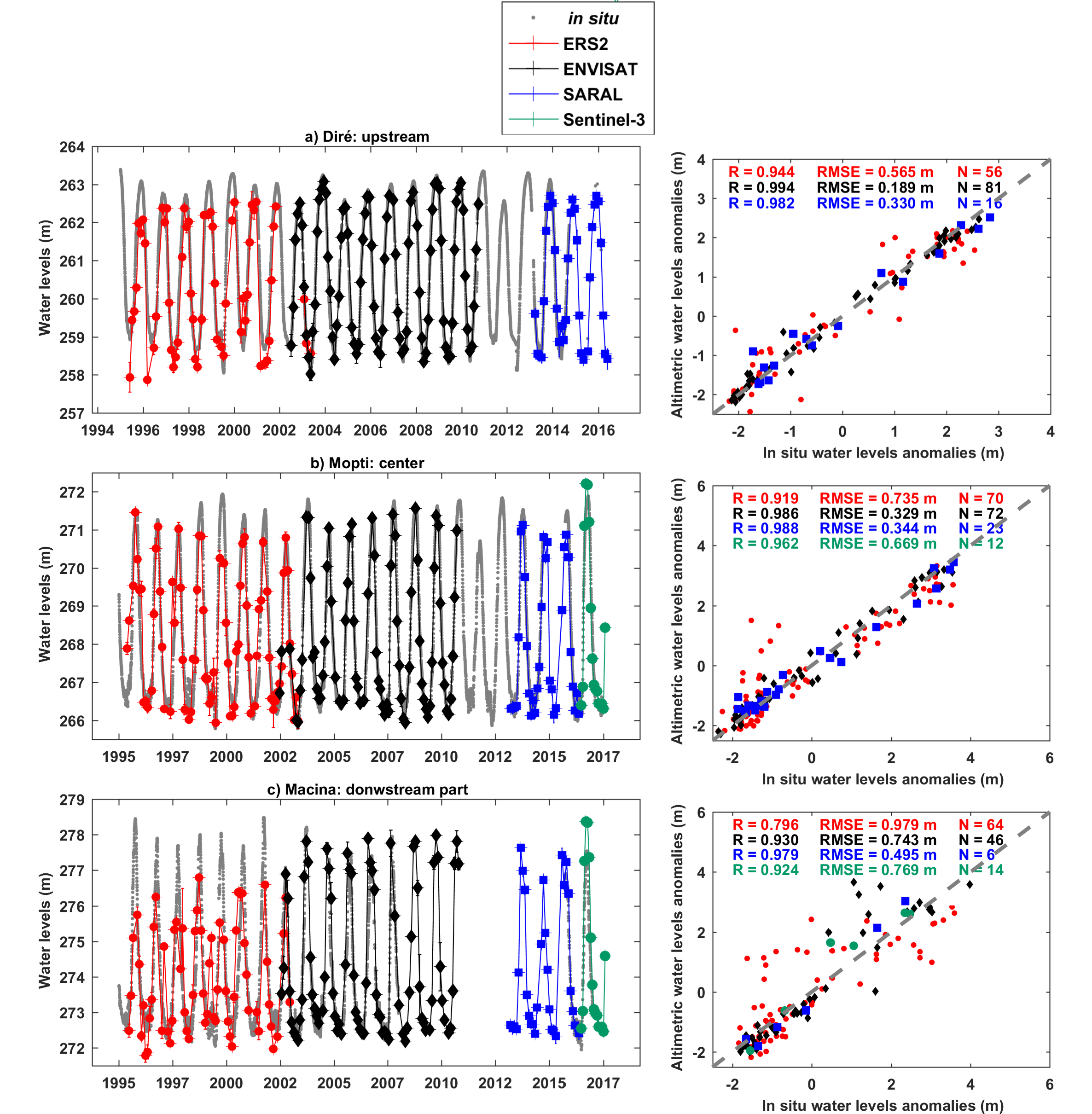
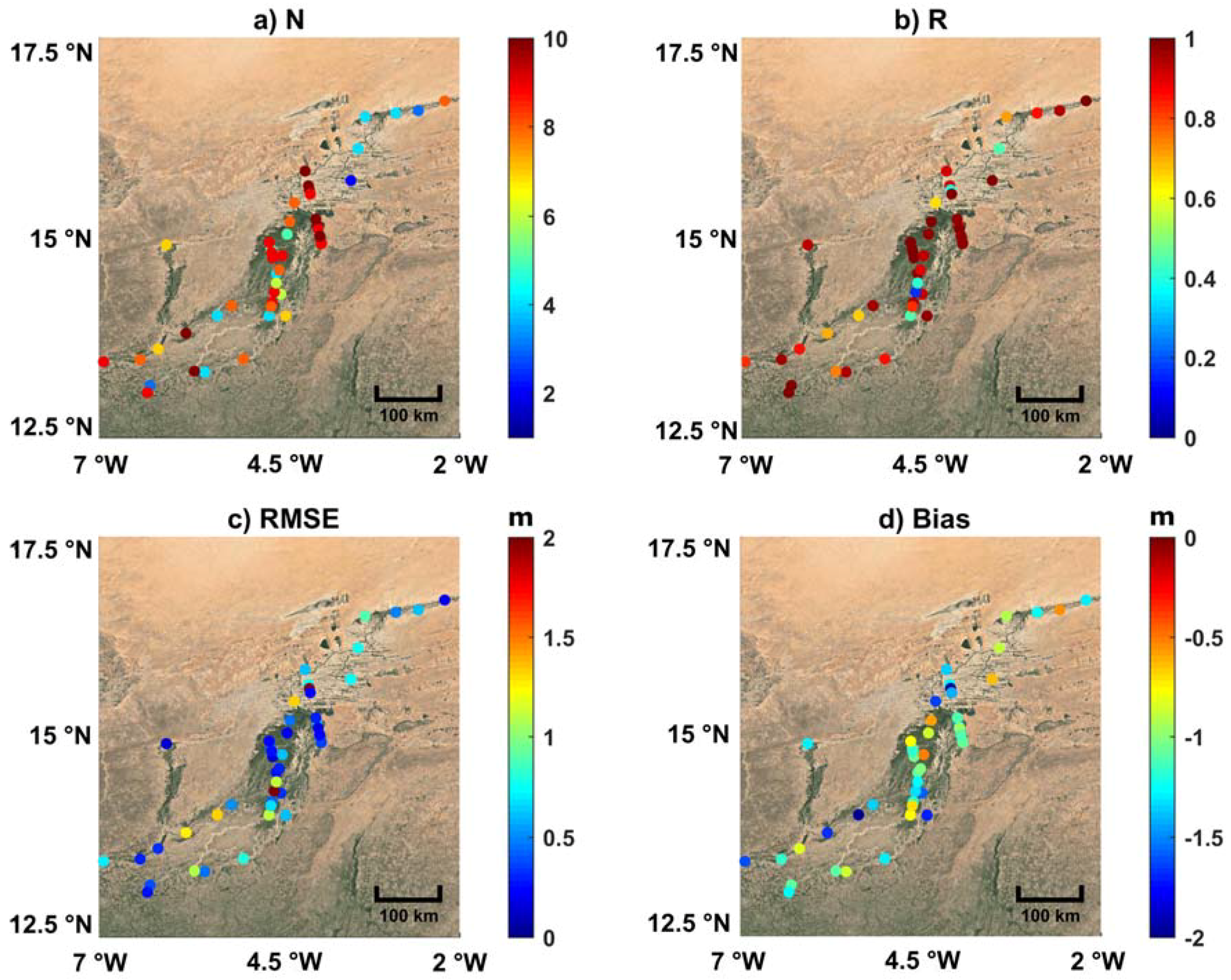
4.1. Direct Validation of the Altimetry-Based Water Stages

The nominal altimetry ground-tracks from ERS-2, ENVISAT, SARAL (35-day repeat orbit), Sentinel-3A (27-day repeat orbit), Jason-1, Jason-2 and Jason-3 (10-day repeat orbit) missions present a large number of cross-sections with river streams and floodplains in the IND (see Figure 3b). A dense network of virtual stations from different missions was defined in the IND (see Table 4). Virtual station (VS) locations in the IND are presented in Figure 3c.
Altimetry-based water levels were compared to water stage records from close in situ gauge. These comparisons were performed for VS located on the rivers and not on the floodplains for distances between the in situ gauge and the VS lower than 100 km. In situ gauge records from 19 stations were used to perform the 89 following comparisons:
  • 19 against ERS-2-based water stages;
  • 32 against ENVISAT-based water stages;
  • 14 against SARAL-based water stages;
  • 3 against Jason-1 and Jason-2-based water stages;
  • 2 against Jason-3-based water stages;
  • 16 against Sentinel-3A-based water stages.
The complete results of these comparisons (distance between the in situ gauge and the VS, number of data used for comparisons (N), RMSE, R and R2) are presented in Tables S1 to S5 for ERS-2, ENVISAT, SARAL, Jason-1/2/3 and Sentinel-3A missions (in supplementary information). The results of these comparisons are also presented as maps in Figure 4 for the altimetry missions that were launched before 2010 (ERS-2, ENVISAT, Jason-1 and 2) and in Figure 5 for the most recent missions. The number of data used for the comparison is, most of the time, statistically significant, except for 15 comparisons against ENVISAT (less than 20 common observations), 4 against SARAL (less than 15 common observations) as well as the whole comparisons against Sentinel-3A as only 16 cycles were used:
  • between 28 and 70 for the 19 ERS-2-based time series of water level (out of 85 available cycles);
  • between 7 and 81 for 32 ENVISAT-based time series of water level (out of 89 available cycles);
  • between 6 and 28 for the 14 SARAL-based time series of water level (out of 35 available cycles);
  • between 46 and 147 for the 3 Jason-1-based time series of water level (out of 262 available cycles);
  • between 37 and 72 for the 3 Jason-2-based time series of water level (out of 303 available cycles);
  • between 45 and 50 for the 2 Jason-3-based time series of water level (out of 55 available cycles);
  • between 3 and 15 for the 16 Sentinel-3A-based time series of water level (out of 16 available cycles).
Very good agreements were generally found between altimetry-based and in situ water stages for all the missions over a total of 89 comparisons performed. Values of R greater than 0.95 were obtained 41 times (45%), between 0.95 and 0.9, 18 times (20%), and between 0.8 and 0.9, 18 times (20%). Correlation coefficients R lower than 0.7 were obtained only 4 times (4%) (Figure 6a). The minimum R value is 0.57. RMSE lower than 0.3 m were obtained 12 times (13%), between 0.3 and 0.5 m, 17 times (19%), between 0.5 and 0.75 m, 29 times (32%) and above 1 m, 19 times (21%) (Figure 6b). Better agreement was found for the recent missions such as SARAL, Jason-3 and Sentinel-3A than for the older ones (ERS-2, ENVISAT, Jason-1 and Jason-2). Focusing on the correlations, for instance R was greater than 0.9 in 10 out of 19 comparisons for ERS-2 (52%), in 19 out of 32 (59%) for ENVISAT, in 10 out of 14 (71%) for SARAL, in 14 out of 16 (88%) for Sentinel-3A, 1 (R = 0.89) out of 3 (33%) for Jason-1, 3 out of 3 for Jason-2 (100%) and 3 out of 3 (100%) for Jason-3 (Tables S1–S5). The first results of the use of Sentinel-3A are very encouraging as only very few cycles were available, keeping in mind that among the three correlation coefficients lower than 0.9, three were already higher than 0.85.
Combining altimetry-based time series of water levels from missions in the same nominal orbits (i.e., ERS-2, ENVISAT and SARAL, and Jason-1, Jason-2 and Jason-3) or at inter-mission cross-overs (ERS-2/ENVISAT/SARAL with Sentinel-3A ground-tracks), multi-mission time series of water levels were obtained. In this latter case, the maximum difference in time between SARAL and Sentinel-3A acquisitions is half the length of the shortest repeat period of the two satellites (i.e., 13 days considering the 27 days of Sentinel-3A repeat period). Inter-mission biases were removed:
  • using the acquisitions made during tandem phases when two missions were in the same orbit a few seconds or minutes apart from each other (e.g., Jason-1 and Jason-2, Jason-2 and Jason-3, ERS-2 and ENVISAT);
  • averaging the acquisitions made during the common period of observations at low water stages (April–May–June) for Sentinel-3A and SARAL;
  • averaging the acquisitions made during low water periods (April–May–June) on different years for ENVISAT (2003–2010) and SARAL (2013–2016).
Low water periods were chosen, rather than high water periods or the complete hydrological cycle, to minimize the effect of the difference in temporal sampling, assuming that water levels are more stable during low water stages.
Examples of multi-mission time series of water levels are presented in Figure 7 and Figure 8 for ERS-2/ENVISAT/SARAL and Sentinel-3A (when there is a cross-over) and for Jason-1, Jason-2 and Jason-3 respectively along with in situ gauge station gauge records of Diré upstream part of the IND, Mopti, central part and Macina, downstream part, over 1995–2017 (Figure 7a–c respectively), and of Macina, over 2002–2017 (Figure 8).
In examples presented in Figure 7, a very good agreement is found between altimetry-based and in situ water stages. There is a gap in the time series between November 2010 and January 2013 as no altimetry mission was in the 35-day repeat orbit during this period. In spite of the distance between the VS and the two first in situ gauge stations (77 and 40 km, with Diré and Mopti stations respectively, but only 1 km from the Macina station under the ERS-2/ENVISAT and SARAL ground-tracks, and 8 km from Macina station under Sentinel-3A ground-tracks), better results were found in the first examples than in the latter one, with higher R2 and lower RMSE for ERS-2 and ENVISAT and similar ones for SARAL and Sentinel-3A. An underestimation of the annual amplitude of the water levels is observed during the ERS-2 observation period. In the example presented in Figure 8, the VS and the Macina in situ gauge station are separated by only 1 km. The quality of the water stage retrieval is increasingly better from Jason-1 to Jason-3. It is important to mention that Jason-1 data contained in the GDR E, released in May 2016, allow the accurate and continuous estimation of water stages over the IND contrary to the previous GDR versions that contained few useful data over land (except over large lakes, see [18,51,52] for instance).

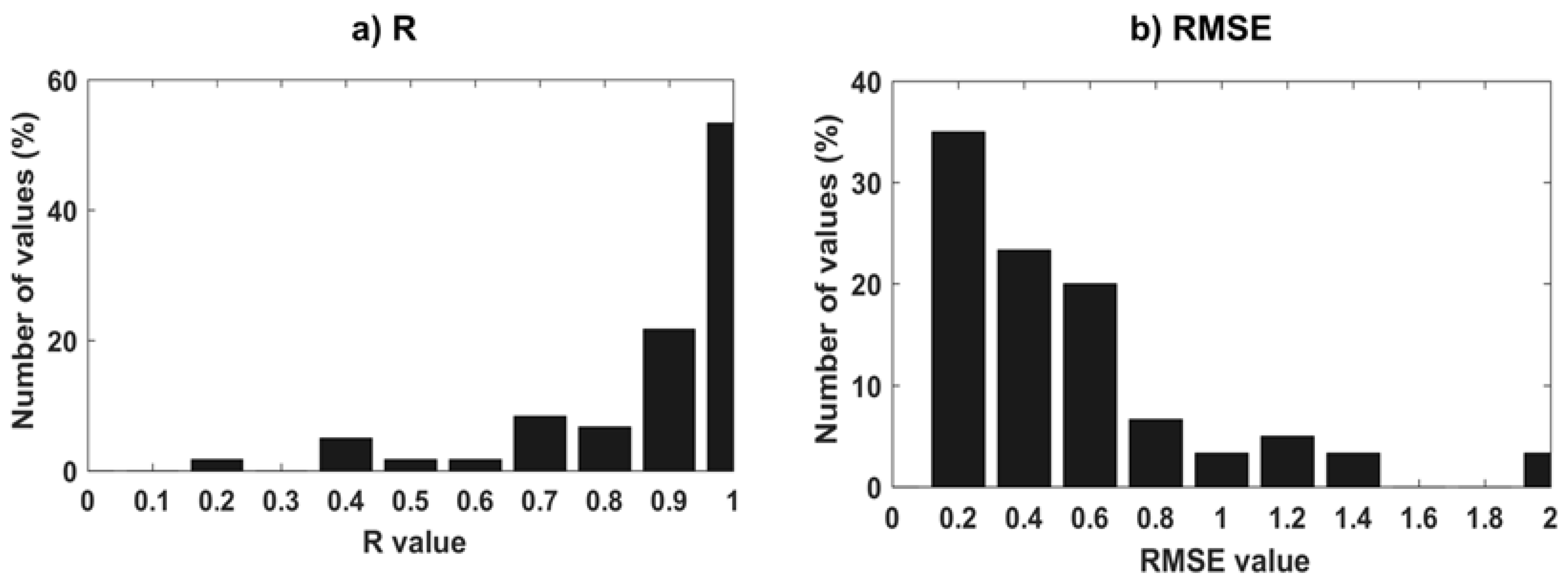
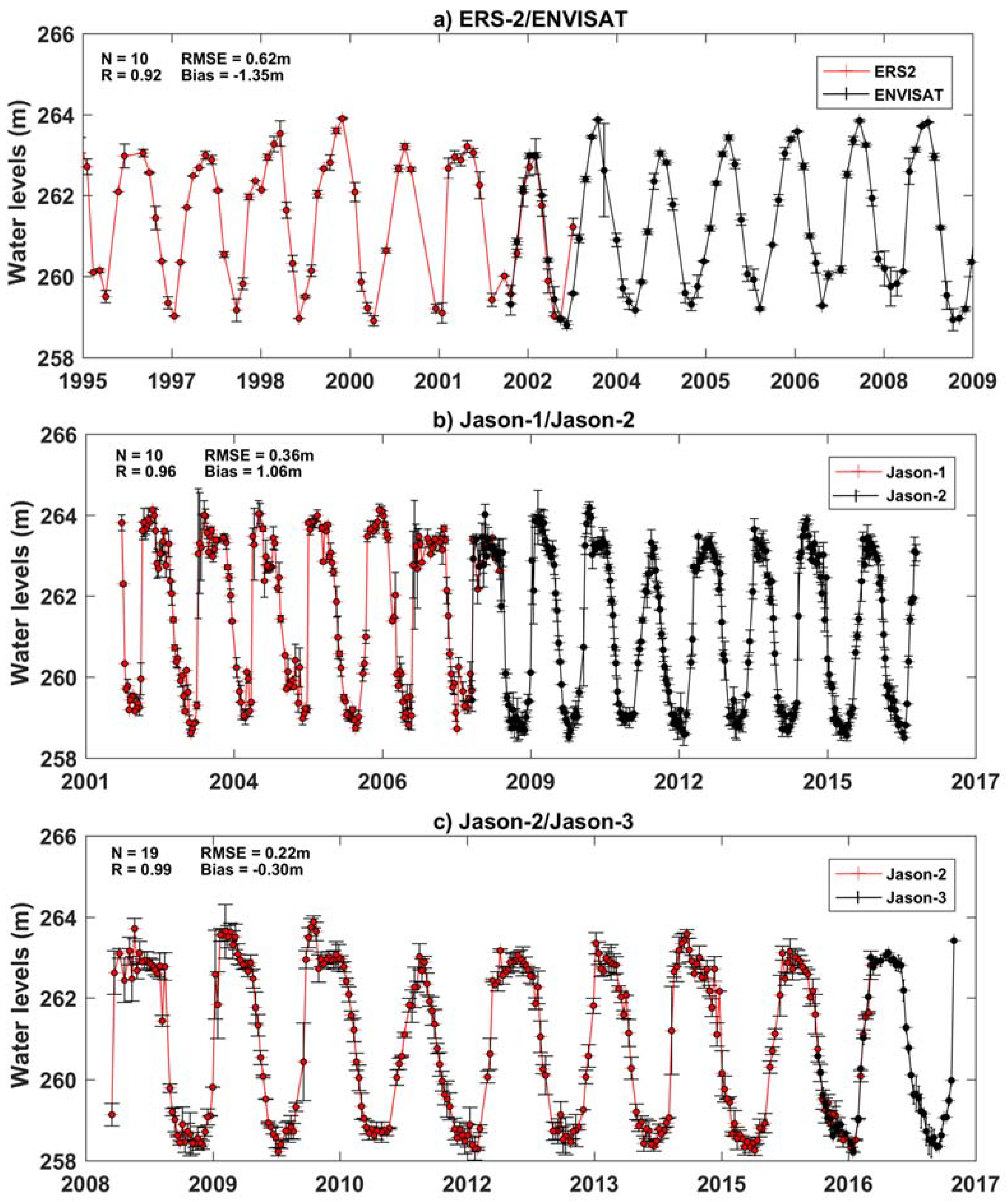
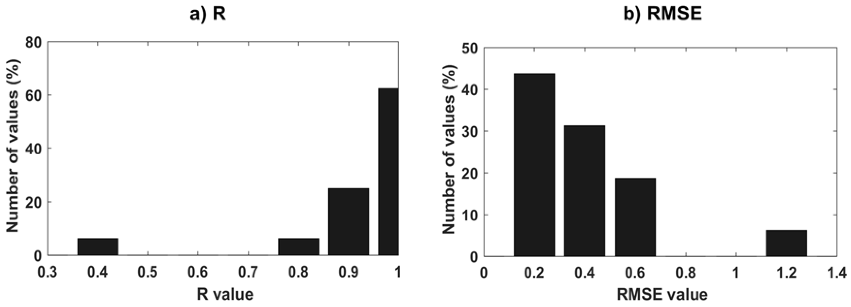
4.2. Intermission Water Stage Comparison

Comparisons between water levels estimated by altimetry missions during their tandem phase (i.e., few cycles during which two missions were orbiting a few minutes apart from one another) were performed between ERS-2 and ENVISAT from June 2002 to July 2003 (11 cycles in common), Jason-1 and Jason-2 from July 2008 to January 2009 (21 cycles in common), Jason-2 and Jason-3 from January to September 2016 (23 cycles in common). They allow the increase of the number of comparisons in the IND, not only on the rivers but also on the wetlands that are monitored using in situ gauges.
A total of 48 comparisons between ERS-2 and ENVISAT-based water levels were performed in the IND with several samples (N) varying from 3 to 11 (Figure 9). On the total number of comparisons between ERS-2 and ENVISAT missions, 22 were performed on more than 8 samples (45%) (Figure 9a). Very good agreement was generally obtained between altimetry-based water stages from the two missions (Figure 9a,b). The value R greater than 0.95 was obtained 24 times (50%), between 0.95 and 0.9, 7 times (15%), and between 0.8 and 0.9, 7 times (15%) (Figure 10a). Correlation coefficients (R) lower than 0.5 were obtained 5 times (10%) (Figure 9b). Values of RMSE lower than 0.3 m were obtained 13 times (27%), between 0.3 and 0.5 m, 10 times (21%), between 0.5 and 0.75 m, 13 times (27%) and above 1 m, 8 times (17%) (Figure 10b). Large biases are observed between ERS-2 and ENVISAT (−1.16 ± 0.38 m on average) (Figure 9d).
A total of 5 and 7 comparisons between Jason-1 and Jason-2, and Jason-2 and Jason-3-based water levels were performed in the IND with several samples (N) varying from 5 to 15 for Jason-1/Jason-2, and from 13 to 22 for Jason-2/Jason-3. Three of these comparisons were performed on more than 10 samples (60%) for Jason-1 (Figure 11a). Very good agreement was generally found between altimetry-based water stages from Jason-1 and 2. Values of R greater than 0.95 were obtained 3 times (60%). In the two other cases, R equal to 0.80 and 0.69 were found (Figure 11b). Values of RMSE lower than 0.3 m were obtained 3 times (60%). In the two other cases, RMSE lower than 0.35 m were found (Figure 11c). Biases between Jason-1 and 2 ranged between 0.34 and 1.06 m (0.75 ± 0.28 m) (Figure 11d).
Better agreement is found between altimetry-based water stages from Jason-2 and 3. Correlation coefficients R greater than 0.95 were obtained in all the cases except one (86%) for which R equals to 0.84 (Figure 12b). Values of RMSE lower than 0.30 m were obtained in all the cases except one (86%) for which RMSE equals to 0.40 m (Figure 12c). Biases between Jason-1 and 2 are very similar, ranging from −0.36 to −0.14 m (−0.27 ± 0.08 m) (Figure 12d).
Examples of time series combining ERS-2 and ENVISAT, Jason-1 and 2, and Jason-2 and 3 are presented on Figure 13a–c. Virtual stations from close locations were chosen: ERS-2/ENVISAT VS 0545-a and Jason-1/Jason-2/Jason-3 VS 046-d. They are located in the upstream part of the IND at an approximate along-stream distance of 45 km. Seasonal amplitudes of between 4 and 5 m are observed during the common period of availability of the different altimetry-based water levels. The agreement is better for the recent missions than for the older ones: R increases from 0.92 to 0.99 whereas RMSE decreases from 0.62 to 0.22 m as well as the bias from −1.35 to 0.36 m. Lower deviations are generally observed on the time series from the more recent missions than other the older ones: 0.13 ± 0.11, 0.13 ± 0.15, 0.19 ± 0.22, 0.21 ± 0.16, 0.15 ± 0.11 m were obtained averaging the mean absolute deviation from individual cycles for ERS-2, ENVISAT, Jason-1, 2 and 3 respectively. Please note that, for readability purpose, biases between the time series were removed in Figure 13.

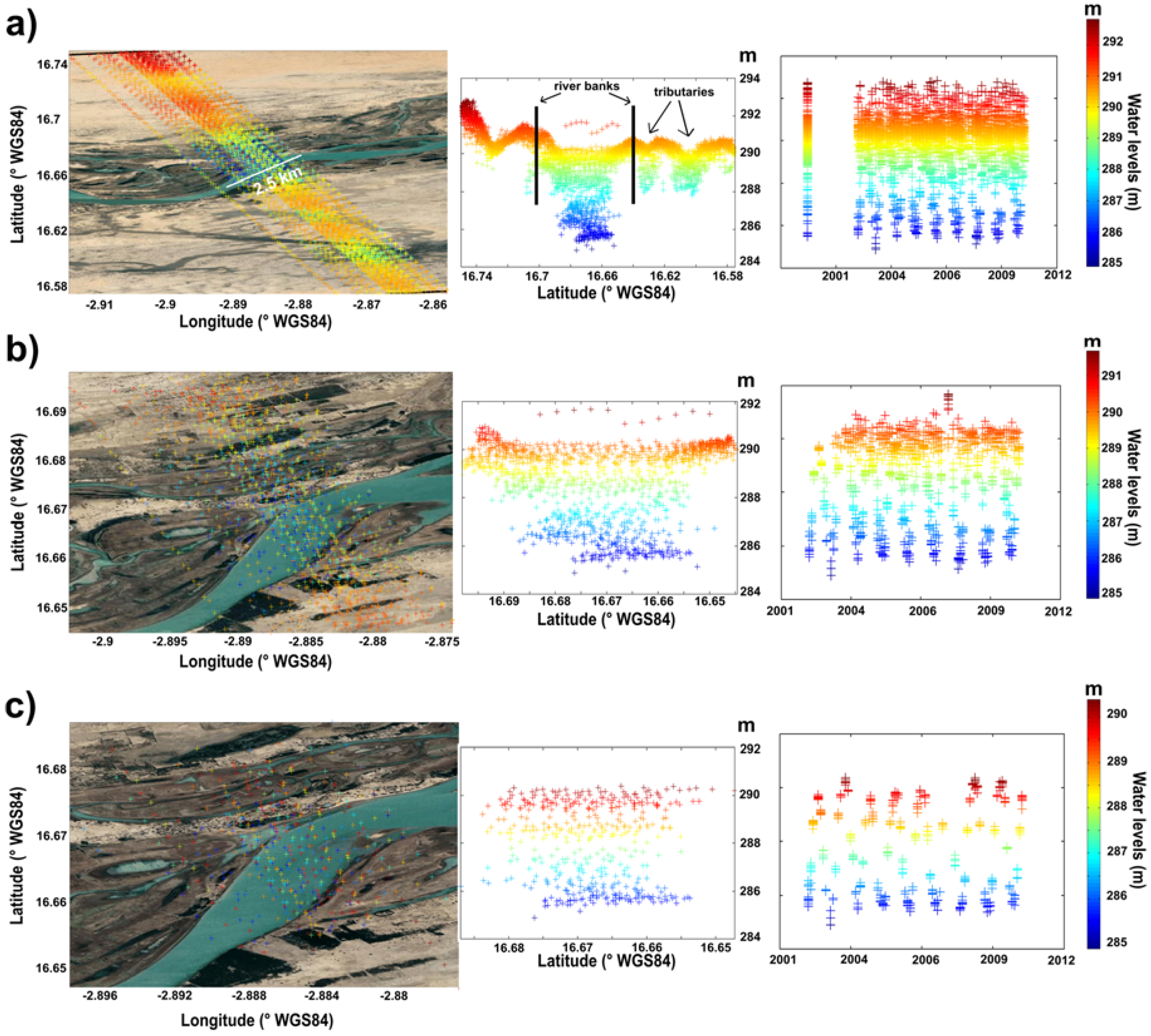
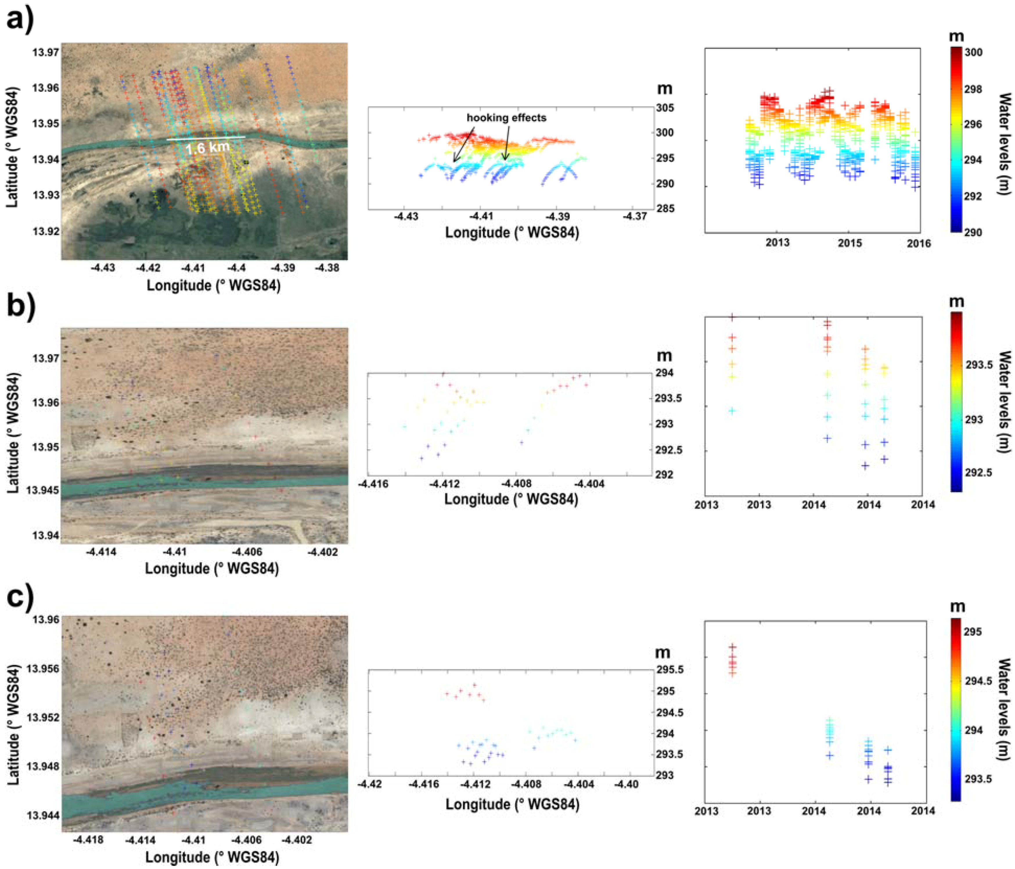
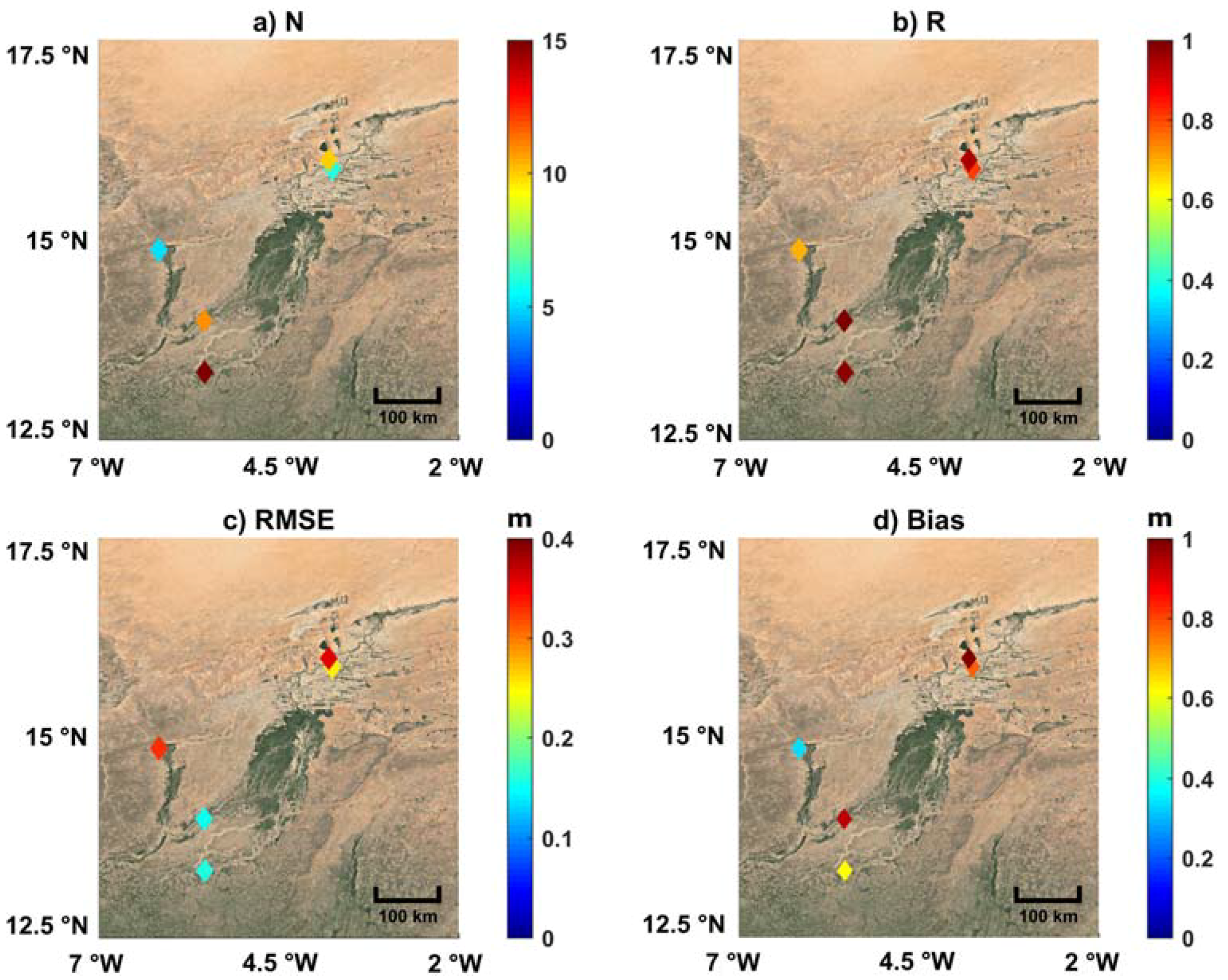
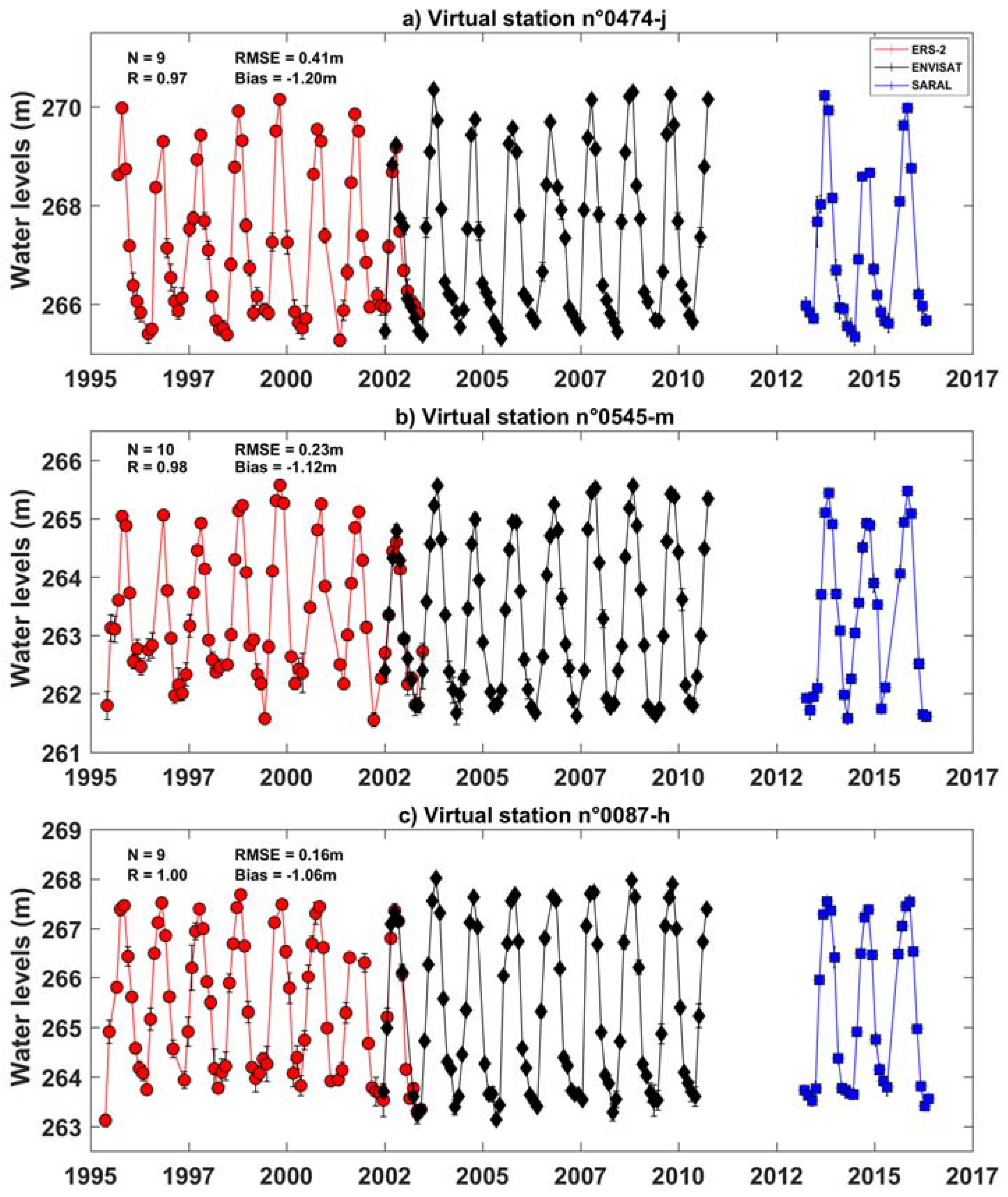
4.3. Multi-Mission Time Series on Floodplains

Floodplains and wetlands are generally not monitored using in situ gauges. Radar altimetry is a unique tool for the long-term observations of the changes in water levels over inundated areas [53,54,55,56,57]. Among the VS defined in the IND, 16 were built in floodplains under ERS-2/ENVISAT/SARAL ground-tracks and 9 under Sentinel-3A ground-tracks, but none under Jason-1, Jason-2 and Jason-3 ground-tracks. Their consistency was checked during the tandem phase between ERS-2 and ENVISAT (Figure 14). Values of R greater than 0.95 were obtained 10 times (63%), between 0.95 and 0.9, twice (12%), and between 0.8 and 0.9, 3 times (19%). However, R lower than 0.5 was obtained once (6%) (Figure 14a). Values of RMSE lower than 0.3 m were obtained 7 times (44%), between 0.3 and 0.5 m, 5 times (31%), between 0.5 and 0.75 m, 3 times (19%) and above 1 m, once (6%) (Figure 14b).
Three examples of multi-mission time series of water levels (corrected for inter-mission bias) over the IND floodplains are presented for VS located in the center, in the north east and in the south (Figure 15a–c respectively). They provide time-variations of water stages between 1995–2016 with the exception of a gap between November 2010 and January 2013.

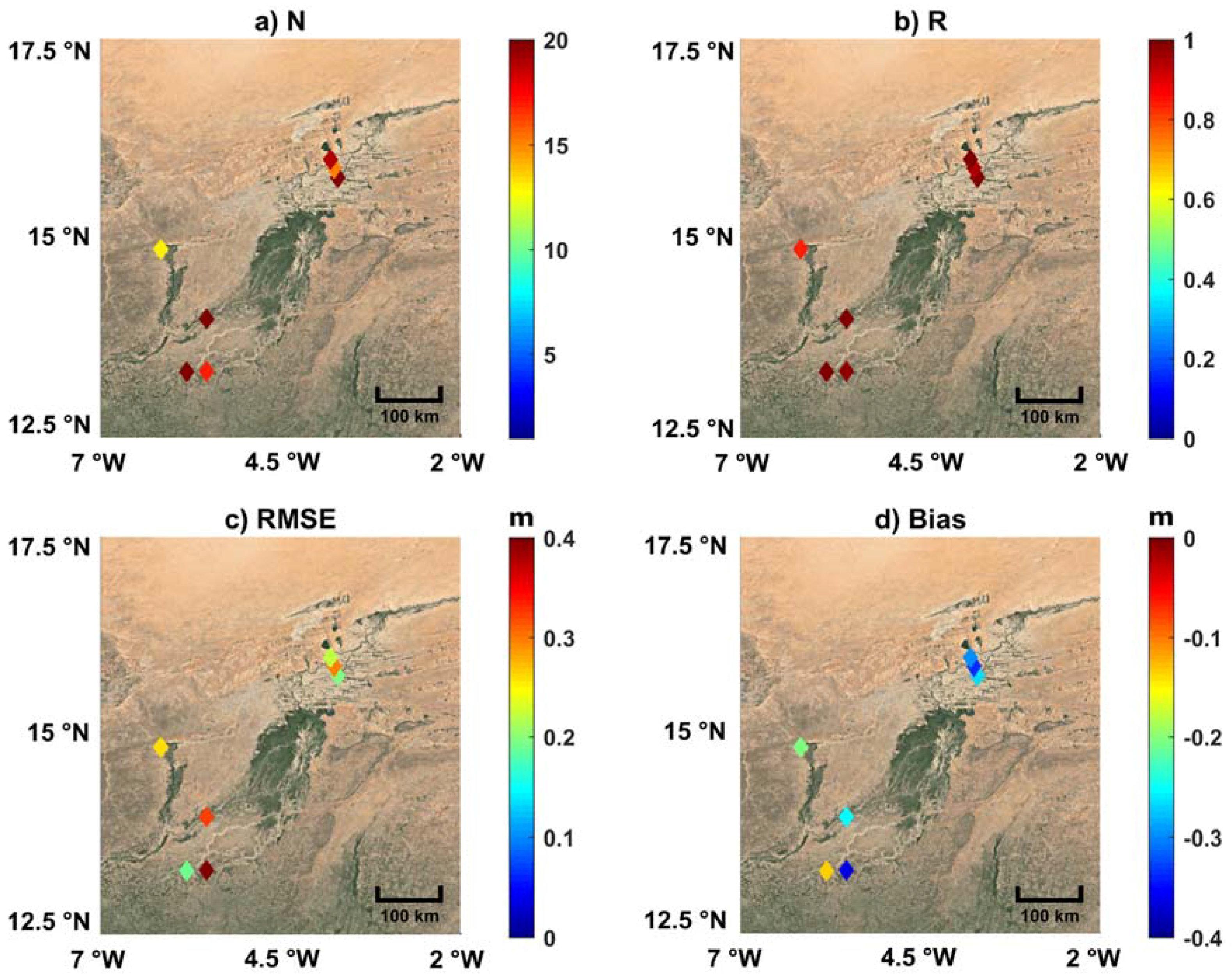
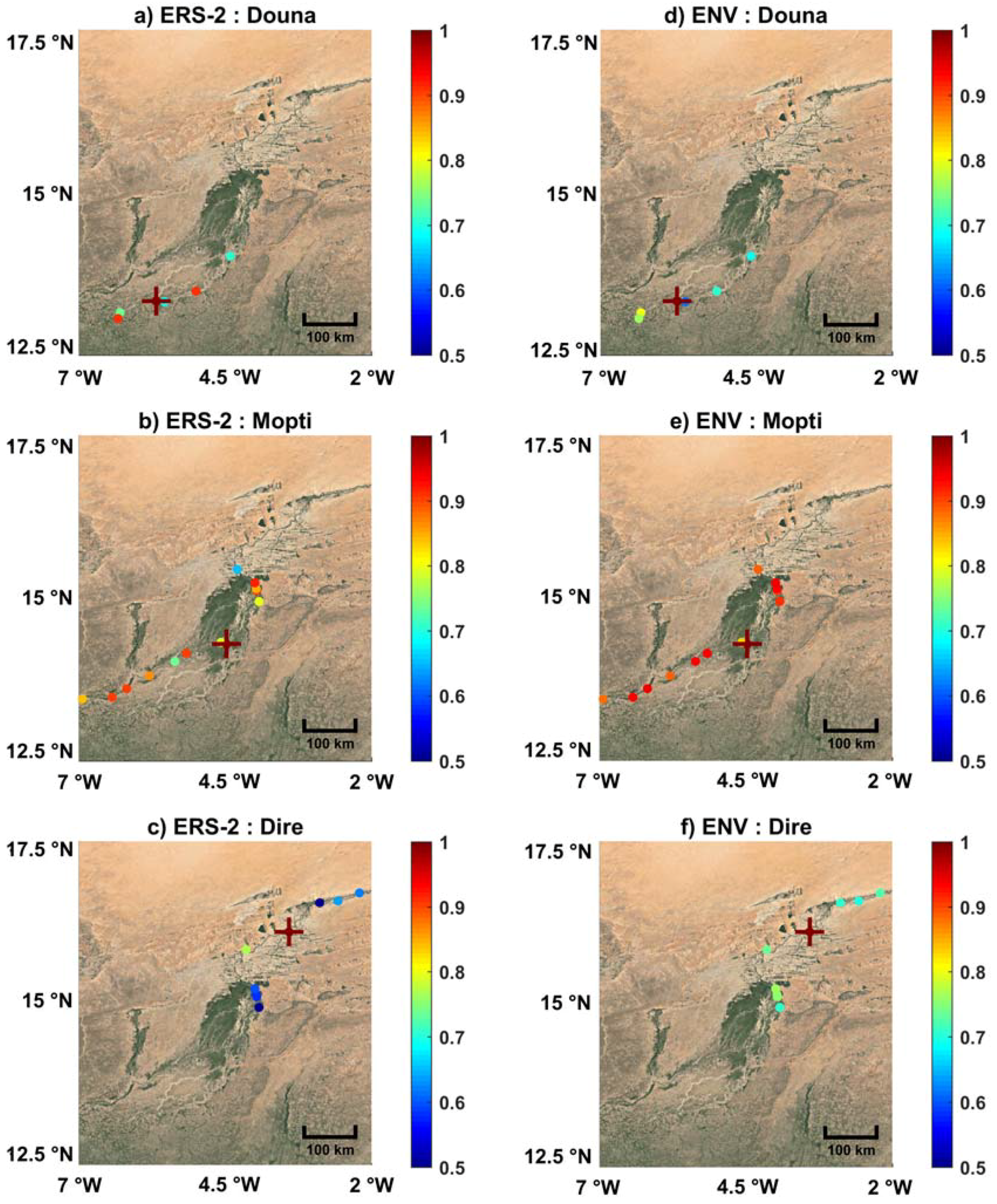
4.4. Consistency of the Altimetry-Based Water Levels in the Inner Niger Delta (IND)

A consistency check was performed between a reference VS located either in Niger River mainstem or in the Bani major tributary and the other VS from the same altimetry mission located upstream and downstream on the same river course estimating the maximum of correlation using the cross-correlation function and the associated time-lag, similarly as in Bogning et al. [29]. Cross-correlation function maxima and associated time-lags are presented for ERS-2 and ENVISAT in Figure 16 and Figure S1 respectively and for SARAL and Sentinel-3A in Figure 17 and Figure S2 respectively for three different VS locations in the IND: near Douna, over the Bani tributary, near Mopti, in the downstream part of the IND, and near Diré in the upstream part of the IND. As the repeat period of these missions is either 35 or 27 days in their nominal orbit, only time-lags of plus or minus one repeat period and a half (i.e., 53 and 41 days) were considered due to the relatively small scale of the IND. Due to the changes of the river features (slope, depth, width, etc.), biases and RMSEs were not computed between the time series of altimetry-based water levels.
Correlation coefficients (R) higher than 0.7 are generally observed for ERS-2 and ENVISAT, except in the upstream part of the delta for ERS-2, with correlation ranging from 0.5 to 0.7 (Figure 16c). Correlations higher than 0.8 are observed in the IND downstream and central parts for ENVISAT (Figure 16). Very high correlations, generally higher than 0.85, especially in the downstream part, except on a few locations, were observed for SARAL and, especially, for Sentinel-3A (Figure 17). No time-lag was observed over the Bani River for none of the altimetry missions (Figures S1a, d and S2a,d). Time lags of plus or minus one cycle were respectively found for the upper and lower stations along the Niger mainstem (Figures S1 and S2).

5. Discussion

The coverage of altimetry tracks from missions of the 35-day (ERS-2/ENVISAT/SARAL) and the 27-day (Sentinel-3A) repeat orbits allows the construction of a dense network of VS on both rivers and floodplains in the IND, completed by a few VS from missions in the 10-day repeat orbit (Figure 3c). Yet, a larger number (more than 15%) of ENVISAT (6) and SARAL-based (62) VS than ERS-2-based (52) ones were built on the ground-tracks of the 35-day repeat orbit. These VS with no valid ERS-2-based water levels are located on the upstream part of the IND for 5 of them, central part for 3 others and downstream part for the last 3 ones.
Due to the relative flatness of the IND, the no-construction of VS cannot be attributed to data losses caused by tracking issues, but to incorrect range estimates. They were likely to be caused by the narrow width of the river streams, especially in the upstream part, where they are generally lower than 300 m. They can also be accounted for the possible complexity of the waveforms (e.g., multi-peaked over areas with several bright targets encompassed in the altimeter footprint such as several river streams that can reach 1 km of width as in the downstream part of the IND, or several floodplain lakes as in the central part).
Comparisons with a high number of in situ gauge records show an overall very good agreement between in situ and altimetry-based water levels, increasingly better for the most recent missions than the older ones. Contrary to what was found in other study areas with variations of topography (e.g., [28,29]), the data used to build the VS were mostly acquired at 330 and 320 MHz Ku chirp bandwidth operation mode by both ERS-2 and ENVISAT (i.e., with the better range resolution in more than 95% of the cases for any VS—Figure 18). This is the reason quite similar results when comparing ERS-2 and ENVISAT-based water stages with in situ water levels were found in terms of R, with generally higher RMSE for ERS-2 (see Figure 4, Tables S1 and S2), and also a good agreement when comparing ERS-2 and ENVISAT-based water levels during their tandem phase, except in terms of bias (Figure 10). In the same orbit, better results were found using SARAL data (Figure 5 and Table S3), as already observed in other river basins, resulting from the use of the Ka-band with its smaller footprint and higher chirp frequency of 500 MHz [29,58].
Very similar numbers of VS were built using Jason-1, Jason-2 and Jason-3 data. The release of the Jason-1 GDR E, which contained valid data over land and not mostly only over large lakes as in the previous versions, allowed the extension of the duration of the time series of water levels over rivers for the missions in the 10-day repeat orbit down to 2001, at the expense of lower accuracy than using Jason-2 and Jason-3 data (Figure 4 and Figure 5 and Table S4). This lower accuracy can be accounted for the small river widths, most of the time lower than 500 m, except in some locations in the downstream part of the IND.
On the contrary, Jason-2 and Jason-3 confirm their great capability for detecting and accurately estimating water levels over narrow rivers, especially over flat areas [28,30]. Comparisons performed during the tandem phase logically confirm the lower agreement between Jason-1 and Jason-2 than between Jason-2 and Jason-3 (Figure 11 and Figure 12). In terms of bias, if high and variable biases were found between Jason-1 and Jason-2-based time series of water levels, much lower ones with low variability were found between Jason-2 and Jason-3 ones during their tandem period. Poseidon-3, on-board Jason-3, is nominally operating in open loop or DIODE/DEM tracking mode over land surfaces, meaning that the reception window is controlled by an a-priori elevation from an along-track DEM loaded in the altimeter [30].
Very good results were also found using one year and a half of measurements from Sentinel-3A, the first altimeter to operate in SAR over all types of surfaces. During this short time period, the results obtained are almost as good as the ones obtained using SARAL, confirming the strong potential of this technique for monitoring inland water stages. This is likely due to the sharper waveform obtained in SAR mode compared with Low Resolution Mode (LRM) [59] as OCOG is particularly well adapted for very specular echoes from a single reflector (e.g., a river stream). On the contrary, less accurate estimates can be expected from multi-peak waveforms.
The consistency of intra-mission water levels derived from radar altimetry measurements was analyzed using cross-correlations for ERS-2, ENVISAT, SARAL and Sentinel-3A. In this case, too, higher correlations were found for the most recent missions operating in (LRM) at Ka band (SARAL) and in SAR at Ku band (Sentinel-3A). Time-lags corresponding to the maximum of cross-correlation (Figures S1 and S2) also showed that there is a time-lag of around two months between the upstream and the downstream part of the IND, in accordance with the water residence time estimated using satellite images [39].

6. Conclusions

An extensive assessment of the performance of almost all the missions put in orbit from ERS-2 to Sentinel-3A was performed over the IND. Around 90 comparisons between in situ and altimetry-based were performed as well as more than 75 intermission comparisons between ERS-2 and ENVISAT, Jason-1 and Jason-2, and Jason-2 and Jason-3. Results of these comparisons show (i) a better agreement between altimetry-derived and in situ water stages over rivers of width varying from a few hundreds of meters to ~1.5 km and floodplains, (ii) an increase in accuracy in water level estimates for the most recent missions such as SARAL, Jason-3 and Sentinel-3A benefiting from the use of the Ka-band for SARAL and of the SAR acquisition mode for Sentinel-3A.
Due to the small number of VS defined on Jason-3 ground-tracks, the DIODE/DEM was not evaluated. Intra-mission consistency check performed on ERS-2, ENVISAT, SARAL and Sentinel-3A missions exhibits a time-lag for the maximum of around 2 months that can be related to the residence time of the water in the IND.
Very good performance of the recently launched altimeter SARAL onboard Sentinel-3A ensures the continuity of the monitoring of the IND whose data density should increase with the launch, in 2018, of Sentinel-3B, in the same orbit as Sentinel-3A but Sentinel-3B flies at ±140° out of phase with Sentinel-3A.
This network of VS will present a strong interest for (i) assessing the impacts of climate variability and human effects (e.g., dam operation and rice production), and (ii) validating the measurement of the future Surface Water and Ocean Topography (SWOT) mission, the first mission to operate in close nadir interferometry SAR for providing elevations in two swaths, to be launched in 2021, on both rivers and floodplains.

Supplementary Materials

The following are available online at https://0-www-mdpi-com.brum.beds.ac.uk/2072-4292/10/6/833/s1, Figure S1: Time-lag corresponding to maxima of cross-correlation between time series of water levels derived from SARAL (left) and SENTINEL-3A (right) data in the IND for three different VS near Douna (a and d), Mopti (b and e) and Diré (c and f). Light blue crosses symbolize the VS chosen as reference (auto-correlation of 1 and time-lag null), Figure S2: Time-lag corresponding to maxima of cross-correlation between time series of water levels derived from SARAL (left) and SENTINEL-3A (right) data in the IND for three different VS near Douna (a and d), Mopti (b and e) and Diré (c and f). Light blue crosses symbolize the VS chosen as reference (auto-correlation of 1 and time-lag null), Table S1: Results of the comparisons between in situ and altimetry water levels derived from ERS-2 mission: number of sample (N), correlation coefficient (R), determination coefficient (R2) and Root Mean Square Error (RMSE), Table S2: Results of the comparisons between in situ and altimetry water levels derived from ENVISAT mission: number of sample (N), correlation coefficient (R), determination coefficient (R2) and Root Mean Square Error (RMSE), Table S3: Results of the comparisons between in situ and altimetry water levels derived from SARAL mission: number of sample (N), correlation coefficient (R), determination coefficient (R2) and Root Mean Square Error (RMSE), Table S4: Results of the comparisons between in situ and altimetry water levels derived from Jason-1, Jason-2 and Jason-3 missions: number of sample (N), correlation coefficient (R), determination coefficient (R2) and Root Mean Square Error (RMSE), Table S5: Results of the comparisons between in situ and altimetry water levels derived from Sentinel-3A mission: number of sample (N correlation coefficient (R), determination coefficient (R2) and Root Mean Square Error (RMSE).

Author Contributions

C.N., F.F., A.T.D. and E.M. designed the study. C.N. processed the altimetry data to produce the time series of water levels. A.T.D. and N.B. provided the in situ data and gave important information on their quality. All of the authors of the present work contributed to the discussion of the results, as well as the writing of the manuscript.

Funding

This study was supported by Centre National d’Etudes Spatiales (CNES) through “Centre de Topographie des Océans et de l’Hydrosphère—CTOH” grant. Cassandra Normandin is supported by Ministère de l’Enseignement Supérieur et de la Recherche through a PhD grant.

Acknowledgments

We thank four anonymous reviewers who helped us improving our manuscript.

Conflicts of Interest

The authors declare no conflict of interest. The founding sponsors had no role in the design of the study; in the collection, analyses, or interpretation of data; in the writing of the manuscript, and in the decision to publish the results.

References

  1. Vörösmarty, C.J.; Green, P.; Salisbury, J.; Lammers, R.B. Global water resources: vulnerability from climate change and population growth. Science 2000, 289, 284–288. [Google Scholar] [CrossRef] [PubMed]
  2. Oki, T.; Kanae, S. Global hydrological cycles and world water resources. Science 2006, 313, 1068–1072. [Google Scholar] [CrossRef] [PubMed]
  3. Haddeland, I.; Heinke, J.; Biemans, H.; Eisner, S.; Flörke, M.; Hanasaki, N.; Konzmann, M.; Ludwig, F.; Masaki, Y.; Schewe, J.; et al. Global water resources affected by human interventions and climate change. Proc. Natl. Acad. Sci. USA 2014, 111, 3251–3256. [Google Scholar] [CrossRef] [PubMed]
  4. Gleick, P.H. Global freshwater resources: soft-path solutions for the 21st century. Science 2003, 302, 1524–1528. [Google Scholar] [CrossRef] [PubMed]
  5. Alsdorf, D.E.; Rodríguez, E.; Lettenmaier, D.P. Measuring surface water from space. Rev. Geophys. 2007, 45, RG2002. [Google Scholar] [CrossRef]
  6. Stammer, D.; Cazenave, A. Satellite Altimetry over Oceans and Land Surfaces; Taylor & Francis: Boca Raton, FL, USA, 2017; ISBN 978-1-4987-4345-7. [Google Scholar]
  7. Crétaux, J.-F.; Nielsen, K.; Frappart, F.; Papa, F.; Calmant, S.; Benveniste, J. Hydrological applications of satellite altimetry: rivers, lakes, man-made reservoirs, inundated areas. In Satellite Altimetry Over Oceans and Land Surfaces; Earth Observation of Global Changes; Stammer, D., Cazenave, A., Eds.; CRC Press: Boca Raton, FL, USA, 2017; pp. 459–504. [Google Scholar]
  8. Morris, C.S.; Gill, S.K. Variation of Great Lakes water levels derived from Geosat altimetry. Water Resour. Res. 1994, 30, 1009–1017. [Google Scholar] [CrossRef]
  9. Birkett, C.M. The contribution of TOPEX/POSEIDON to the global monitoring of climatically sensitive lakes. J. Geophys. Res. 1995, 100204, 25179–25204. [Google Scholar] [CrossRef]
  10. Koblinsky, C.J.; Clarke, R.T.; Brenner, A.C.; Frey, H. Measurement of river level variations with satellite altimetry. Water Resour. Res. 1993, 29, 1839–1848. [Google Scholar] [CrossRef]
  11. Birkett, C.M. Contribution of the TOPEX NASA Radar Altimeter to the global monitoring of large rivers and wetlands. Water Resour. Res. 1998, 34, 1223. [Google Scholar] [CrossRef]
  12. Frappart, F.; Calmant, S.; Cauhopé, M.; Seyler, F.; Cazenave, A. Preliminary results of ENVISAT RA-2-derived water levels validation over the Amazon basin. Remote Sens. Environ. 2006, 100. [Google Scholar] [CrossRef] [Green Version]
  13. Frappart, F.; Legrésy, B.; Niño, F.; Blarel, F.; Fuller, N.; Fleury, S.; Birol, F.; Calmant, S. An ERS-2 altimetry reprocessing compatible with ENVISAT for long-term land and ice sheets studies. Remote Sens. Environ. 2016, 184. [Google Scholar] [CrossRef]
  14. Baup, F.; Frappart, F.; Maubant, J. Use of satellite altimetry and imagery for monitoring the volume of small lakes. In International Geoscience and Remote Sensing Symposium (IGARSS); 2014. [Google Scholar]
  15. Sulistioadi, Y.B.; Tseng, K.-H.; Shum, C.K.; Hidayat, H.; Sumaryono, M.; Suhardiman, A.; Setiawan, F.; Sunarso, S. Satellite radar altimetry for monitoring small rivers and lakes in Indonesia. Hydrol. Earth Syst. Sci. 2015, 19, 341–359. [Google Scholar] [CrossRef]
  16. Frappart, F.; Papa, F.; Malbeteau, Y.; León, J.G.J.G.; Ramillien, G.; Prigent, C.; Seoane, L.; Seyler, F.; Calmant, S. Surface freshwater storage variations in the orinoco floodplains using multi-satellite observations. Remote Sens. 2015, 7, 89–110. [Google Scholar] [CrossRef]
  17. da Silva, J.S.; Calmant, S.; Seyler, F.; Moreira, D.M.; Oliveira, D.; Monteiro, A. Radar Altimetry Aids Managing Gauge Networks. Water Resour. Manag. 2014, 28, 587–603. [Google Scholar] [CrossRef]
  18. Birkett, C.; Reynolds, C.; Beckley, B.; Doorn, B. From Research to Operations: The USDA Global Reservoir and Lake Monitor. In Coastal Altimetry; Springer Berlin Heidelberg: Berlin/Heidelberg, Germany, 2011; pp. 19–50. [Google Scholar]
  19. Ričko, M.; Birkett, C.M.; Carton, J.A.; Crétaux, J.-F. Intercomparison and validation of continental water level products derived from satellite radar altimetry. J. Appl. Remote Sens. 2012, 6, 61710. [Google Scholar] [CrossRef] [Green Version]
  20. Cretaux, J.-F.; Berge-Nguyen, M.; Leblanc, M.; Rio, R.A.D.; Delclaux, F.; Mognard, N.; Lion, C.; Pandey, R.-K.; Tweed, S.; Calmant, S.; et al. Flood mapping inferred from remote sensing data. Int. Water Technol. J. 2011, 1, 48–62. [Google Scholar]
  21. Goita, K.; Diepkile, A.T. Radar altimetry of water level variability in the Inner Delta of Niger River. In Proceedings of the IEEE International Geoscience and Remote Sensing Symposium, Munich, Germany, 22–27 July 2012; pp. 5262–5265. [Google Scholar]
  22. Frappart, F.; Fatras, C.; Mougin, E.; Marieu, V.; Diepkilé, A.T.; Blarel, F.; Borderies, P. Radar altimetry backscattering signatures at Ka, Ku, C, and S bands over West Africa. Phys. Chem. Earth 2015, 83–84, 96–110. [Google Scholar] [CrossRef]
  23. Tarpanelli, A.; Amarnath, G.; Brocca, L.; Massari, C.; Moramarco, T. Discharge estimation and forecasting by MODIS and altimetry data in Niger-Benue River. Remote Sens. Environ. 2017, 195, 96–106. [Google Scholar] [CrossRef]
  24. Tourian, M.J.; Schwatke, C.; Sneeuw, N. River discharge estimation at daily resolution from satellite altimetry over an entire river basin. J. Hydrol. 2017, 546, 230–247. [Google Scholar] [CrossRef]
  25. Chelton, D.B.; Ries, J.C.; Haines, B.J.; Fu, L.-L.; Callahan, P.S. Chapter 1 Satellite Altimetry. In Satellite Altimetry and Earth Sciences A Handbook of Techniques and Applications; Elsevier, 2001; Volume 69, pp. 1–131. ISBN 0074-6142. [Google Scholar]
  26. Frappart, F.; Blumstein, D.; Cazenave, A.; Ramillien, G.; Birol, F.; Morrow, R.; Rémy, F. Satellite Altimetry: Principles and Applications in Earth Sciences. In Wiley Encyclopedia of Electrical and Electronics Engineering; John Wiley & Sons, Inc.: Hoboken, NJ, USA, 2017; pp. 1–25. ISBN 047134608X. [Google Scholar]
  27. Frappart, F.; Papa, F.; Marieu, V.; Malbeteau, Y.; Jordy, F.; Calmant, S.; Durand, F.; Bala, S. Preliminary Assessment of SARAL/AltiKa Observations over the Ganges-Brahmaputra and Irrawaddy Rivers. Mar. Geod. 2015, 38. [Google Scholar] [CrossRef]
  28. Biancamaria, S.; Frappart, F.; Leleu, A.S.; Marieu, V.; Blumstein, D.; Desjonquères, J.D.; Boy, F.; Sottolichio, A.; Valle-Levinson, A. Satellite radar altimetry water elevations performance over a 200 m wide river: Evaluation over the Garonne River. Adv. Sp. Res. 2017, 59, 128–146. [Google Scholar] [CrossRef]
  29. Bogning, S.; Frappart, F.; Blarel, F.; Niño, F.; Mahé, G.; Bricquet, J.P.; Seyler, F.; Onguéné, R.; Etamé, J.; Paiz, M.C.; Braun, J.J. Monitoring water levels and discharges using radar altimetry in an ungauged river basin: The case of the Ogooué. Remote Sens. 2018, 10, 350. [Google Scholar] [CrossRef]
  30. Biancamaria, S.; Schaedele, T.; Blumstein, D.; Frappart, F.; Boy, F.; Desjonquères, J.D.; Pottier, C.; Blarel, F.; Niño, F. Validation of Jason-3 tracking modes over French rivers. Remote Sens. Environ. 2018, 209, 77–89. [Google Scholar] [CrossRef]
  31. Frappart, F.; Roussel, N.; Biancale, R.; Martinez Benjamin, J.J.; Mercier, F.; Perosanz, F.; Garate Pasquin, J.; Martin Davila, J.; Perez Gomez, B.; Gracia Gomez, C.; et al. The 2013 Ibiza Calibration Campaign of Jason-2 and SARAL Altimeters. Mar. Geod. 2015, 38. [Google Scholar] [CrossRef]
  32. Vu, P.; Frappart, F.; Darrozes, J.; Marieu, V.; Blarel, F.; Ramillien, G.; Bonnefond, P.; Birol, F. Multi-Satellite Altimeter Validation along the French Atlantic Coast in the Southern Bay of Biscay from ERS-2 to SARAL. Remote Sens. 2018, 10, 93. [Google Scholar] [CrossRef]
  33. Jekeli, C. Geometric Reference System in Geodesy; Division of Geodesy and Geospatial Science School of Earth Sciences, Ohio State University: Columbus, OH, USA, 2006. [Google Scholar]
  34. Salameh, E.; Frappart, F.; Marieu, V.; Spodar, A.; Parisot, J.P.; Hanquiez, V.; Turki, I.; Laignel, B. Monitoring sea level and topography of coastal lagoons using satellite radar altimetry: The example of the Arcachon Bay in the Bay of Biscay. Remote Sens. 2018, 10, 297. [Google Scholar] [CrossRef]
  35. Mahé, G.; Bamba, F.; Soumaguel, A.; Orange, D.; Olivry, J.C. Water losses in the inner delta of the River Niger: water balance and flooded area. Hydrol. Process. 2009, 23, 3157–3160. [Google Scholar] [CrossRef]
  36. De Noray, M.-L. Delta intérieur du fleuve Niger au Mali–quand la crue fait la loi: l’organisation humaine et le partage des ressources dans une zone inondable à fort contraste. VertigO-la Rev. électronique en Sci. l’ Environ. 2003, 4, 1–9. [Google Scholar] [CrossRef]
  37. Zwarts, L. The Niger, A Lifeline: Effective Water Management in the Upper Niger Basin; RIZA: Lelystad, 2005; ISBN 978-90-807150-6-6. [Google Scholar]
  38. Jones, K.; Lanthier, Y.; van der Voet, P.; van Valkengoed, E.; Taylor, D.; Fernández-Prieto, D. Monitoring and assessment of wetlands using Earth Observation: The GlobWetland project. J. Environ. Manag. 2009, 90, 2154–2169. [Google Scholar] [CrossRef] [PubMed]
  39. Bergé-Nguyen, M.; Crétaux, J.-F. Inundations in the Inner Niger Delta: Monitoring and Analysis Using MODIS and Global Precipitation Datasets. Remote Sens. 2015, 7, 2127–2151. [Google Scholar] [CrossRef]
  40. Ogilvie, A.; Belaud, G.; Delenne, C.; Bailly, J.-S.; Bader, J.-C.; Oleksiak, A.; Ferry, L.; Martin, D. Decadal monitoring of the Niger Inner Delta flood dynamics using MODIS optical data. J. Hydrol. 2015, 523, 368–383. [Google Scholar] [CrossRef]
  41. Benveniste, J.; Roca, M.; Levrini, G.; Vincent, P.; Baker, S.; Zanife, O.; Zelli, C.; Bombaci, O. The radar altimetry mission: RA-2, MWR, DORIS and LRR. ESA Bull. 2001, 106, 25101–25108. [Google Scholar]
  42. Steunou, N.; Desjonquères, J.D.; Picot, N.; Sengenes, P.; Noubel, J.; Poisson, J.C. AltiKa Altimeter: Instrument Description and In Flight Performance. Mar. Geod. 2015, 38, 22–42. [Google Scholar] [CrossRef]
  43. Taylor, P.; Perbos, J.; Escudier, P.; Parisot, F.; Zaouche, G.; Vincent, P.; Menard, Y.; Manon, F.; Kunstmann, G.; Royer, D.; et al. Jason-1: Assessment of the System Performances Special Issue: Jason-1 Calibration/Validation. Mar. Geod. 2003, 26, 37–41. [Google Scholar] [CrossRef]
  44. Desjonquères, J.D.; Carayon, G.; Steunou, N.; Lambin, J. Poseidon-3 Radar Altimeter: New Modes and In-Flight Performances. Mar. Geod. 2010, 33, 53–79. [Google Scholar] [CrossRef]
  45. Donlon, C.; Berruti, B.; Buongiorno, A.; Ferreira, M.H.; Féménias, P.; Frerick, J.; Goryl, P.; Klein, U.; Laur, H.; Mavrocordatos, C.; et al. The Global Monitoring for Environment and Security (GMES) Sentinel-3 mission. Remote Sens. Environ. 2012, 120, 37–57. [Google Scholar] [CrossRef]
  46. Wingham, D.J.; Rapley, C.G.; Griffiths, H. New Techniques in Satellite Altimeter Tracking Systems. Proc. IGARSS Symp. Zurich 1986, 1339–1344. [Google Scholar]
  47. Frappart, F.; Do Minh, K.; L’Hermitte, J.; Cazenave, A.; Ramillien, G.; Le Toan, T.; Mognard-Campbell, N. Water volume change in the lower Mekong from satellite altimetry and imagery data. Geophys. J. Int. 2006, 167. [Google Scholar] [CrossRef]
  48. Santos da Silva, J.; Calmant, S.; Seyler, F.; Rotunno Filho, O.C.; Cochonneau, G.; Mansur, W.J. Water levels in the Amazon basin derived from the ERS 2 and ENVISAT radar altimetry missions. Remote Sens. Environ. 2010, 114, 2160–2181. [Google Scholar] [CrossRef]
  49. Cartwright, D.E.; Edden, A.C. Corrected Tables of Tidal Harmonics. Geophys. J. R. Astron. Soc. 1973, 33, 253–264. [Google Scholar] [CrossRef]
  50. Wahr, J.M. Deformation induced by polar motion. J. Geophys. Res. 1985, 90, 9363. [Google Scholar] [CrossRef]
  51. Crétaux, J.F.; Jelinski, W.; Calmant, S.; Kouraev, A.; Vuglinski, V.; Bergé-Nguyen, M.; Gennero, M.C.; Nino, F.; Abarca Del Rio, R.; Cazenave, A.; Maisongrande, P. SOLS: A lake database to monitor in the Near Real Time water level and storage variations from remote sensing data. Adv. Sp. Res. 2011, 47, 1497–1507. [Google Scholar] [CrossRef]
  52. Frappart, F.; Biancamaria, S.; Normandin, C.; Blarel, F.; Bourrel, L.; Aumont, M.; Azemar, P.; Vu, P.-L.; Le Toan, T.; Lubac, B.; et al. Influence of recent climatic events on the surface water storage of the Tonle Sap Lake. Sci. Total Environ. 2018, 636, 1520–1533. [Google Scholar] [CrossRef]
  53. Frappart, F.; Papa, F.; Famiglietti, J.S.; Prigent, C.; Rossow, W.B.; Seyler, F. Interannual variations of river water storage from a multiple satellite approach: A case study for the Rio Negro River basin. J. Geophys. Res. Atmos. 2008, 113. [Google Scholar] [CrossRef] [Green Version]
  54. Lee, H.; Shum, C.K.; Yi, Y.; Ibaraki, M.; Kim, J.W.; Braun, A.; Kuo, C.Y.; Lu, Z. Louisiana wetland water level monitoring using retracked TOPEX/POSEIDON altimetry. Mar. Geod. 2009, 32, 284–302. [Google Scholar] [CrossRef]
  55. Frappart, F.; Papa, F.; Güntner, A.; Werth, S.; Santos da Silva, J.; Tomasella, J.; Seyler, F.; Prigent, C.; Rossow, W.B.; Calmant, S.; Bonnet, M.-P. Satellite-based estimates of groundwater storage variations in large drainage basins with extensive floodplains. Remote Sens. Environ. 2011, 115. [Google Scholar] [CrossRef] [Green Version]
  56. da Silva, J.S.; Seyler, F.; Calmant, S.; Filho, O.C.R.; Roux, E.; Araújo, A.A.M.; Guyot, J.L. Water level dynamics of Amazon wetlands at the watershed scale by satellite altimetry. Int. J. Remote Sens. 2012, 33, 3323–3353. [Google Scholar] [CrossRef]
  57. Zakharova, E.A.; Kouraev, A.V.; Rémy, F.; Zemtsov, V.A.; Kirpotin, S.N. Seasonal variability of the Western Siberia wetlands from satellite radar altimetry. J. Hydrol. 2014, 512, 366–378. [Google Scholar] [CrossRef]
  58. Bonnefond, P.; Verron, J.; Aublanc, J.; Babu, K.; Bergé-Nguyen, M.; Cancet, M.; Chaudhary, A.; Crétaux, J.-F.; Frappart, F.; Haines, B.; et al. The Benefits of the Ka-Band as Evidenced from the SARAL/AltiKa Altimetric Mission: Quality Assessment and Unique Characteristics of AltiKa Data. Remote Sens. 2018, 10, 83. [Google Scholar] [CrossRef]
  59. Keith Raney, R. The delay/doppler radar altimeter. IEEE Trans. Geosci. Remote Sens. 1998, 36, 1578–1588. [Google Scholar] [CrossRef]
Figure 1. The different steps of the altimetry data using Multi-mission Altimetry Processing Software (MAPS). First, a rough selection of the altimetry data (represented with crosses of color) is performed: (a) all altimetry data located a few kilometers away from the center of the river are selected (left panel), the major topographic features, such hills, river banks, tributaries, etc. can be identified (central panel), temporal variations of the altimetry signal cannot be related to any hydrological signal (right panel). Then, a more accurate selection is made; (b) the number of data is decreasing and outliers are removed (left panel), the shape of the river and its temporal variations in width (central panel) and height (left panel) becomes clearer. This process is repeated until final selection is achieved; (c) all subfigures are derived from the MAPS Graphical User Interface (GUI).
Remotesensing 10 00833 g001
Figure 2. Example of the hooking correction. (a) On a rough selection, parabolic profiles in different cycles were identified. (b) Zooming on them, it appears that they are responsible for deviation of several tenths of centimeters of the river levels. (c)Once the correction of the hooking effect is applied, the deviation is reduced to a maximum of a couple of tenths cm).
Remotesensing 10 00833 g002
Figure 3. (a) Location of the IND in Africa; (b) Altimetry tracks over the IND from European Remote-Sensing Satellite-2 (ERS-2), ENVIronment SATellite (ENVISAT), Satellite with Argos and ALtika (SARAL) (blue dots), Jasons-1/Jason-2/Jason-3 (yellow dots) and Sentinel-3A (red dots); and (c) Location of virtual stations to calculate water levels (colored circles) using altimetry data and in situ gauge stations (black diamonds) in IND.
Remotesensing 10 00833 g003
Figure 4. Comparisons between in situ and altimetry water levels for several missions (a) ERS-2 and Jason-1 data and (b) ENVISAT and Jason-2. For each comparison, the number of samples (N), correlation (R), and RMSE is presented. Diamonds points correspond to Jason data and circles with black contours to ERS-2/ENVISAT.
Remotesensing 10 00833 g004
Figure 5. Comparisons between in situ and altimetry water levels for several missions (a) SARAL and Jason-3 data and (b) Sentinel-3A. For each comparison, the number of samples (N), correlation (R), and RMSE is presented. Diamonds points correspond to Jason data and circles with black contours to SARAL/Sentinel-3A.
Remotesensing 10 00833 g005
Figure 6. Histograms of (a) correlations and (b) RMSE between altimetry-based and in situ water stages for all missions.
Remotesensing 10 00833 g006
Figure 7. Altimetry-based water levels from 1995 to 2017 from ERS-2/ENVISAT/SARAL/Sentinel-3A (red/black/blue/green respectively) and in situ (grey) data (left). Scatter plots of water levels anomalies from radar altimetry and in situ gauge stations at (a) Diré (upstream IND), (b) Mopti (center IND) and (c) Macina (downstream IND).
Remotesensing 10 00833 g007
Figure 8. Altimetry-based water levels from 2002 to 2017 from Jason-1/Jason-2/Jason-3 (red/black/blue respectively) and in situ water levels (light green) data (left). Scatter plots of water levels anomalies from radar altimetry and in situ gauge stations at Macina (right figure, downstream IND).
Remotesensing 10 00833 g008
Figure 9. Comparisons between ERS-2 and ENVISAT water levels in terms of (a) number of samples (N), (b) correlation (R), (c) RMSE, and (d) bias.
Remotesensing 10 00833 g009
Figure 10. Histograms of (a) correlation coefficients and (b) RMSE for ERS-2/ENVISAT intermission water stages comparisons.
Remotesensing 10 00833 g010
Figure 11. Comparisons between Jason-1 and Jason-2 water levels in terms of (a) number of samples (N); (b) correlation (R); (c) RMSE; and (d) bias.
Remotesensing 10 00833 g011
Figure 12. Comparisons between Jason-2 and Jason-3 water levels in terms of (a) number of samples (N); (b) correlation (R); (c) RMSE and (d) bias.
Remotesensing 10 00833 g012
Figure 13. Intermission quality time series: (a) for the VS 0545-a located in the upstream part in the IND between ERS-2/ENVISAT; (b) for the VS 046-d (upstream part) between Jason-1/Jason-2; and (c) for the VS 046-d between Jason-2/Jason-3. The two VS are separated by 45 km.
Remotesensing 10 00833 g013
Figure 14. Histograms of (a) R and (b) RMSE for ERS-2/ENVISAT intermission water stages comparisons on floodplains virtual stations.
Remotesensing 10 00833 g014
Figure 15. Water levels time series on floodplains derived from radar altimetry multi-mission (ERS-2/ENVISAT and SARAL) from 1995 to 2016 at 3 different locations in the Inner Niger Delta: the center of the delta (a); the north eastern (b) and the southern (c) parts.
Remotesensing 10 00833 g015
Figure 16. Maxima of cross-correlation between time series of water levels derived from ERS-2 (left) and ENVISAT (right) data in the IND for three different VS near Douna (a,d); Mopti (b,e) and Diré (c,f). Red crosses symbolize the VS chosen as reference (auto-correlation of 1).
Remotesensing 10 00833 g016
Figure 17. Maxima of cross-correlation between time series of water levels derived from SARAL (left) and Sentinel-3A (right) data in the IND for three different VS near Douna (a,d); Mopti (b,e) and Diré (c,f). Red crosses symbolize the VS chosen as reference (auto-correlation of 1).
Remotesensing 10 00833 g017
Figure 18. Percentage of acquisition in the different Ku chirp bandwidth operation mode for each VS in the IND for ENVISAT at 320 MHz (a); at 80 MHz; (b) and at 20 MHz; (c) ERS-2 at 330 MHz (d) and at 82.5 MHz (e).
Remotesensing 10 00833 g018
Table 1. Major characteristics of the high-precision radar altimetry missions used in this study.
MissionJason-1/2/3ERS-2
ENVISAT
SARALSentinel-3A
InstrumentPoseidon-2
Poseidon-3
Poseidon-3B
Radar Altimeter (RA)
Radar Altimeter (RA-2)
AltiKaSar Radar Altimeter (SRAL)
Space agencyCentre National d’Etudes Spatiales (CNES), National Aeronautics and Space Administraion (NASA)European Space Agency (ESA)CNES, Indian Space Research Organization (ISRO)European Space Agency (ESA)
Operation2001–2013
Since 2008
Since 2016
1995–2003
2002–2012
Since 2013Since 2016
Acquisition modeLow Resolution Mode (LRM)LRMLRMPseudo Low Resolution Mode (PLRM), SAR
AcquisitionAlong-trackAlong-trackAlong-trackAlong-track
Frequency (GHz)13.575 (Ku)
5.3 (C)
13.8 (Ku)
13.575 (Ku)
3.2 (S)
35.75 (Ka)13.575 (Ku)
5.41 (C)
Altitude (km)1315800800814.5
Orbit inclination (°)6698.5598.5598.65
Repetitively (days)9.9156353527
Equatorial cross-track separation (km)3157575104
Table 2. Major characteristics of the high-precision radar altimetry missions used in this study.
Altimetry MissionJason-1Jason-2Jason-3ERS-2ENVISATSARALSentinel-3A
GDREDDCentre de Topographie des Océans et de l’Hydrosphère (CTOH) [13]V2.1TESA IPF 06.07 land
Along-track sampling20 Hz20 Hz20 Hz20 Hz18 Hz40 Hz20 Hz
RetrackerICEICEICEICE-1ICE-1ICE-1Offset Centre of gravity (OCOG)
ΔRionoGIM-based
ΔRdryEuropean Centre for Medium-Range Weather Forecasts (ECMWF)-based using Digital Elevation Model (DEM)ECMWF-based using h from altimeterECMWF-based using DEM
ΔRwetECMWF-based using DEM
ΔRsolid EarthBased on Catwright et al. [49]
ΔRpoleBased on Wahr et al. [50]
Table 3. List of in situ gauge stations in the IND used this study.
In Situ Gauge StationLongitude (°)Latitude (°)Validation Period
Akka−4.2315.391992–2017
Diondiori−4.7814.612008–2010
Diré−3.3816.271991–2017
Douna−5.9013.221991–2004
Goundam−3.6516.422009–2017
Kakagnan−4.3314.932008–2010
Kara−5.0114.161992–2011
Kirango−6.0713.72015–2017
Konna−3.914.951992–1999
Koryoumé−3.0316.671992–2017
Macina−5.2914.141991–2017
Mopti−4.1814.481991–2017
Sévéri−4.1914.752008–2010
Sormé−4.414.872008–2010
Sossobé−4.6714.562008–2010
Tilembeya−4.9814.151991–2006
Toguéré Kou−4.5914.932008–2010
Tonka−3.7616.111991–2017
Tou−4.5214.132008–2010
Table 4. Number of virtual stations defined in the IND for each mission.
MissionERS-2ENVISATSARALSentinel-3AJason-1Jason-2Jason-3
Number of virtual stations (VS)52636231889

