Landslide Monitoring Using Multi-Temporal SAR Interferometry with Advanced Persistent Scatterers Identification Methods and Super High-Spatial Resolution TerraSAR-X Images

Abstract

Landslides are one of the most common and dangerous threats in the world that generate considerable damage and economic losses. An efficient landslide monitoring tool is the Differential Synthetic Aperture Radar Interferometry (DInSAR) or Persistent Scatter Interferometry (PSI). However, landslides are usually located in mountainous areas and the area of interest can be partially or even heavily vegetated. The inherent temporal decorrelation that dramatically reduces the number of Persistent Scatters (PSs) of the scene limits in practice the application of this technique. Thus, it is crucial to be able to detect as much PSs as possible that can be usually embedded in decorrelated areas. High resolution imagery combined with efficient pixel selection methods can make possible the application of DInSAR techniques in landslide monitoring. In this paper, different strategies to identify PS Candidates (PSCs) have been employed together with 32 super high-spatial resolution (SHR) TerraSAR-X (TSX) images, staring-spotlight mode, to monitor the Canillo landslide (Andorra). The results show that advanced PSI strategies (i.e., the temporal sub-look coherence (TSC) and temporal phase coherence (TPC) methods) are able to obtain much more valid PSs than the classical amplitude dispersion ($D_A$) method. In addition, the TPC method presents the best performance among all three full-resolution strategies employed. The SHR TSX data allows for obtaining much higher densities of PSs compared with a lower-spatial resolution SAR data set (Sentinel-1A in this study). Thanks to the huge amount of valid PSs obtained by the TPC method with SHR TSX images, the complexity of the structure of the Canillo landslide has been highlighted and three different slide units have been identified. The results of this study indicate that the TPC approach together with SHR SAR images can be a powerful tool to characterize displacement rates and extension of complex landslides in challenging areas.

1. Introduction

Every year, with the onset of rains and snow melting, landslides represent one of the major natural threats to human life and infrastructures in natural and urbanized environments. In this context, different surveying techniques, such as inclinometers, extensometers, piezometers, jointmeters, photogrammetry, LiDAR or Global Positioning Satellite System, are typically employed to address landslide monitoring problems [1,2,3,4,5,6,7,8]. Nonetheless, these conventional techniques present several limitations. They are labor intensive, expensive and usually require skillful users for data interpretation. Moreover, they typically provide poor spatial sampling and coverage, which hinder the characterization of complex landslides. Finally, some of these techniques require the direct installation of devices over the landslide surface, which could be a complex task, sometimes impossible to fulfill, in hard-to-reach locations. During the last decade, Synthetic Aperture Radar (SAR) Differential Interferometry (DInSAR) techniques based on space-borne SAR sensors have matured to a widely used geodetic tool for the accurate monitoring of complex displacement phenomena with millimetric accuracy [9,10,11,12,13]. Concretely, the new generation of X-band SAR sensors, like the German TerraSAR-X and TanDEM-X satellites or the Italian constellation Cosmo-Skymed, have led to a scientific breakthrough presenting a lower revisiting time (up to few days) and an improved spatial resolution (even below the meter), compared with their predecessors ERS-1/2, ENVISAT-ASAR and RADARSAT-1 or the recently Sentinel-1, which worked at the C-band.

Despite all these clear advantages, DInSAR solutions present some limitations, especially for the X-band, over vegetated scenarios in mountainous environments, where landslides typically occur. The DInSAR technique takes advantage of a time-series of SAR images but not all pixels of the image are useful for interferometric processing. Only those pixels with enough phase quality along the whole observing period, i.e., the Persistent Scatterers (PSs), can be used as measurement points (MPs) to derive ground displacement. These PSs, which usually correspond to man-made structures (like buildings, bridges or roads), rocky areas and bare surfaces with no vegetation, are usually scarce in mountainous areas [14,15]. In addition, severe limitations arise from temporal decorrelation over vegetated areas, snow episodes typical in mountainous regions, layover and shadowing effects caused by SAR geometrical distortions, the presence of tropospheric atmospheric artifacts or when rapid displacements are faced, making the processing in such areas difficult and challenging at the same time. Finally, it must be taken into account that SAR sensors are only sensitive to the satellite-to-target component of displacement, i.e., line of sight (LOS) direction, which may notably differ from the real one. The measured displacement will be in fact a projection of the real one [9,12]. Many DInSAR, also known as Persistent Scatters Interferometry (PSI), techniques and algorithms, which share similar principles, have been developed. They have been tested in the last twenty years using many different sensors, either orbital, airborne or ground-based, and over many different scenarios, making this technique a powerful and reliable tool for monitoring any kind of ground motion episodes [14,15,16,17,18,19,20,21].

Large landslides constitute a very specific and challenging scenario for DInSAR. As they are located in mountainous areas and the displacement is usually down-slope, the landslides have to be mostly oriented east to west in order to be sensitive to the displacement if polar orbital sensors are going to be used [9,10]. Not all landslides are suitable for being monitored with orbital SAR. On the one hand, to avoid problems with phase ambiguity, the displacement rate of the landslide must be small enough, let us say a few decimetres per year (depending on the wavelength and revisiting period of the radar). In other words, the SAR interferometry is suitable for monitoring landslides “Very slow” to “Extremely slow” according to the standard landslide classifications [22,23]. In addition, foreshortening and layover can jeopardize the performance of the DInSAR processing so the selection of the proper acquisition geometry is also crucial. In order to reduce geometric distortion and, at the same time, maximize the projection of the landslide displacement to the LOS, it is advisable to observe, if possible, the landslide from behind, as it has been done in this paper. However, each case can be different from the other and so it would require a detailed analysis considering the landslide particularities and the surrounding topography [9,10,12,24]. Atmospheric artifacts, caused by both tropospheric stratification and turbulent component, can contaminate the interferometric phase and, as they can be strongly correlated with the topography, they can also be difficult to remove [25,26,27,28,29]. Finally, a landslide can present a quite complex behaviour with different sliding units moving at different velocity rates. A good density of PS is required in order to be able to delimit and characterize the behaviour of the different local displacements, so it would be necessary to use a PSI strategy able to select as much pixels as possible at full resolution in areas where most of the pixels will be severely decorrelated [9,10]. It is evident that the chances of detecting small and isolated PSs within decorrelated areas will arise as the resolution of the images employed increases [11,30,31].

With super high-resolution (SHR) data, the classical Gaussian scattering model used to model speckle is not always fulfilled since it is possible to find resolution cells with few scatterers [24,32]. This approach is known as partially developed speckle [33,34]. In the situation of having an isolated scatterer within the resolution cell, the value is given by the deterministic impulse response of the SAR system, i.e., by a bidimensional sinc response [24,35]. These types of scatterers typically correspond to man-made structures, outcrops, exposed rocks, etc. These objects can be exploited as opportunistic high-quality points for displacement monitoring applications. Of course, in high-resolution SAR images, it is more probable to have this situation in natural environments [11,30]. Taking into account the previous considerations, landslide monitoring will be greatly benefited by the usage of SHR data.

In this paper, 32 Staring Spotlight TerraSAR-X images (acquired from July 2014 to November 2016, with a resolution of 0.23 m in azimuth and 0.59 m in range) and three full-resolution PSI approaches (i.e., the classical amplitude dispersion [14], the temporal sub-look coherence (TSC) [36,37] and the temporal phase coherence (TPC) [38] methods) are employed to monitor a complex landslide located in El Forn de Canillo (Andorran Pyrenees). Although the advantages of the Staring Spotlight TerraSAR-X SAR data have been demonstrated by different applications such as absolute height estimation [39] and measuring rates of archaeological looting [40], the examples in terms of PSI landslide monitoring are still rare. To our knowledge, the work presented in this paper is the first attempt to study the possible benefits of SHR SAR images for landslide monitoring, especially regarding the aspects of pixel density and capability to detect PSs within decorrelated areas. At the same time, the above-mentioned three PS strategies have also been tested to determine the one most suited for this kind of scenario.

The paper is organized as follows. The landslide’s geological setting and employed dataset are firstly presented in Section 2. Section 3 introduces the procedures of PSI, where the different strategies are described. Section 4 presents the landslide monitoring results with TerraSAR-X images, which are analyzed and compared with GPS measurements to evaluate their reliability. After that, in Section 5 the advantages of SHR SAR images are highlighted by the comparison of the results with those achieved with lower resolution sensors, Sentinel-1 in this case. Finally, Section 6 presents the conclusions.

2. Study Area and Dataset

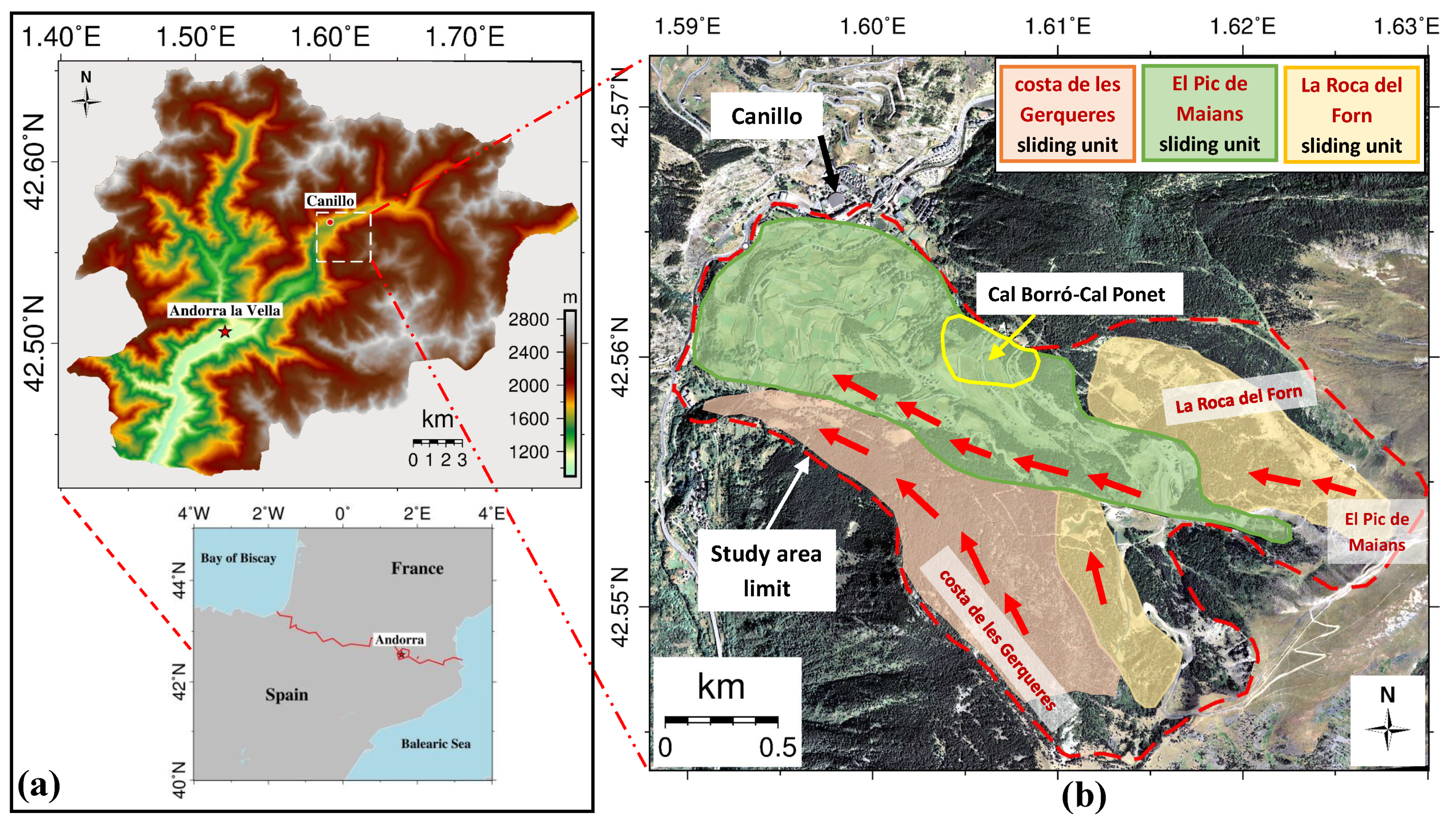
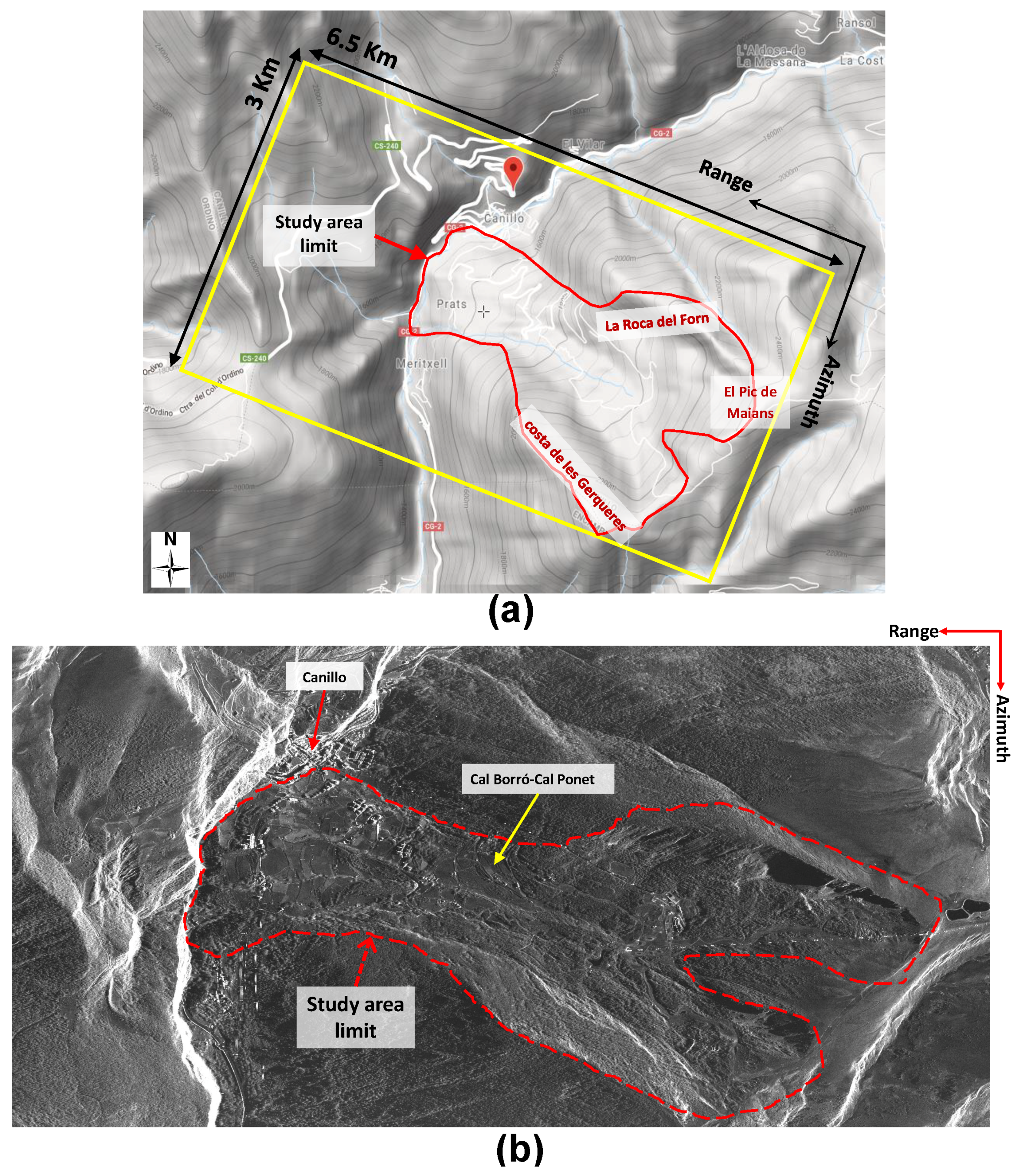
2.1. Canillo Landslide

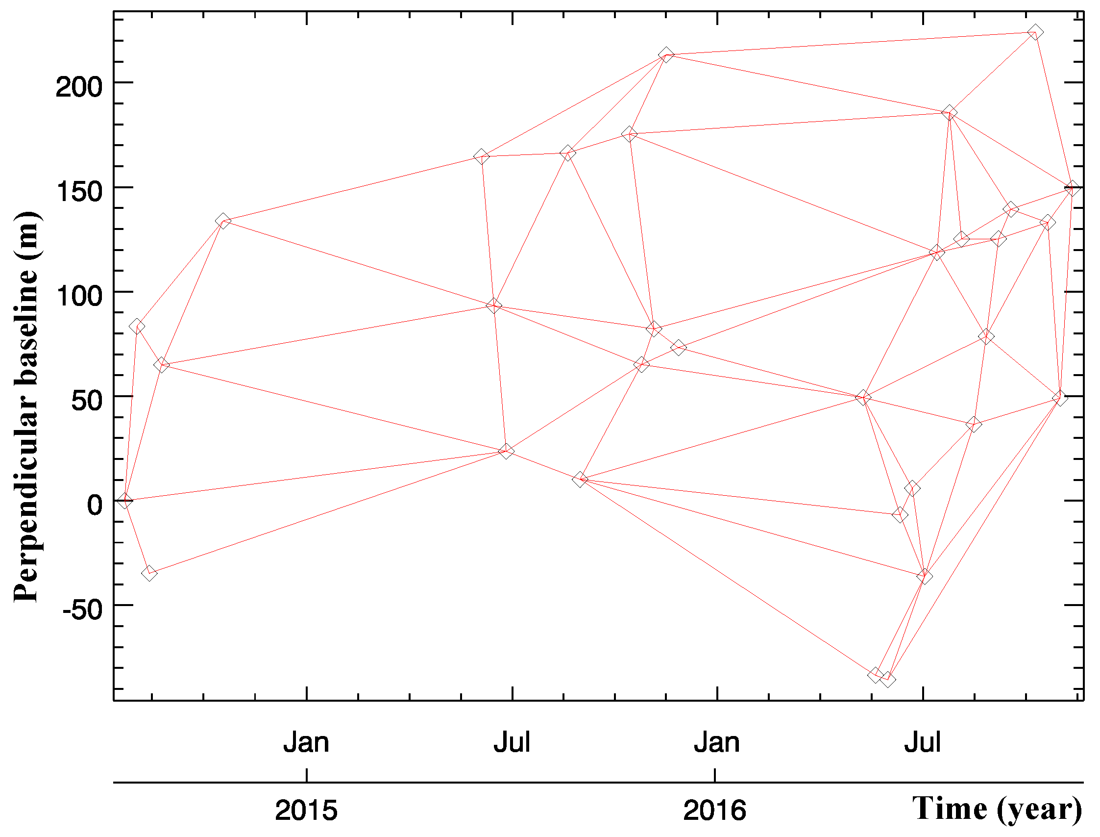
The area selected in this paper corresponds to one of the biggest and ancient landslides of the Andorran Pyrenees. It is located at El Forn de Canillo ($42.{5610}^{\circ }$N, $1.{6018}^{\circ }$E) in the Principality of Andorra, which is a mountainous country between Spain and France in the Central Pyrenees, as Figure 1a shows. It is a complex structure with deposits composed of overlapped colluvial layers generated by different landslide episodes. It was firstly described by Corominas and Alonso in 1984 [41] and has been the subject of several studies where its morphology, failure mechanisms and evolution has been deeply analyzed. The hillslope of El Forn de Canillo is composed by a sequence of slides and earth-flows with a complex structure, which affects an estimated mass at around $3\times {10}^8$ m${}^3$. In this context, different ancient sliding units were identified in 1994 by Santacana [42] (see Figure 1b). The first one corresponds to a slide originated in the area of Pla del Géspit-Costa de les Gerqueres, located in the southeast of the landslide, which reaches the foot of the hillside. A second event was originated under El Pic de Maians, reaching the height of 1540 m, and which overlaps with the previous sliding unit, closing in the Valira river valley. Finally, a third rockslide with a lower extension originated on the hillside known as La Roca del Forn, in the northeast side of the hillslope, was identified. Recent local instabilities have been identified in different locations within the landslide mass [43]. The landslide of El Forn de Canillo was originated as the result of the hillside destabilization, due to a decompression phenomenon after the removal of the Valira Glacier during the Pleistocene, after the Maximum Ice Extent. The Valira River has been progressively eroding the base of the whole mass without reaching the bedrock, and thus originating the landslide [42].

In front of some evidence of displacement (geomorphological signs of instability and some cracking in the road pavement and in a hydroelectric channel that crosses the Forn de Canillo), the authorities promoted several actions in the year 2000 for the management of their geo-hazard threats leading to the monitoring of El Forn de Canillo. Between the years 2007 and 2009, a network of geotechnical devices, including inclinometers, rod extensometers and piezometers, were installed over the landslide surface to characterize and understand the dynamics of the sliding mass. A total of 10 boreholes, reaching typically a depth between 40 and 60 m, were drilled and equipped with this instrumentation [43,44]. The readings recorded have provided evidence that, in addition to a residual movement of some millimeters per year in the main body of the slide, the most active part of the landslide corresponds to the secondary landslide of Cal Borró-Cal Ponet. This area registered a velocity up to roughly 2 cm/month between May and June 2009 when intense sudden rain events and snow melting occurred [44].

2.2. SAR Dataset

In this study, the slides’ motion is monitored with 32 Staring Spotlight TerraSAR-X (TSX) Single Look Complex (SLC) SAR images. This imaging mode is the classical spotlight mode and it is able to enhance the azimuth resolution, compared with the stripmap mode, by steering the antenna in azimuth to a rotation center within the imaged scene [45]. The coverage of the SAR images is around 6.5 km in length and 3 km in width, which has been plotted in Figure 2a (yellow rectangle). The SAR image main parameters are presented in

Table 1. Main parameters of the employed Staring Spotlight TerraSAR-X images. Heading and LOS angles defined clockwise with respect to the north.

Parameter	Value
Acquisition Period	22 July 2014–15 November 2016
Heading Angle	189.8 (degree)
LOS Angle	279.8 (degree)
Incidence Angle	39 (degree)
Azimuth Resolution	0.23 (m)
Slant Range Resolution	0.59 (m)
Wavelength	3.1 (cm)
Revisit Cycle	11 (day)

.

An amplitude image of the SAR dataset is presented in Figure 2b. As it can be seen, the SAR images’ geometric distortion effects (i.e., foreshortening, shadow and layover) are not serious within the study area limit. The extended brighter areas of the image are those affected by the foreshortening and layover, due to the steepest topography. Dark areas are those affected by shadowing. This is favoured by a certain parallelism between the topography of the slope and the LOS from the satellite, thanks to its descending flight direction. The landslide is partially vegetated. Only a few strong scatterers (man-made structures, like buildings and roads, or bare rocks) are sparsely distributed within the study area limit, as is also visible in Figure 1b, thus making it challenging to monitor this landslide with conventional PSI techniques.

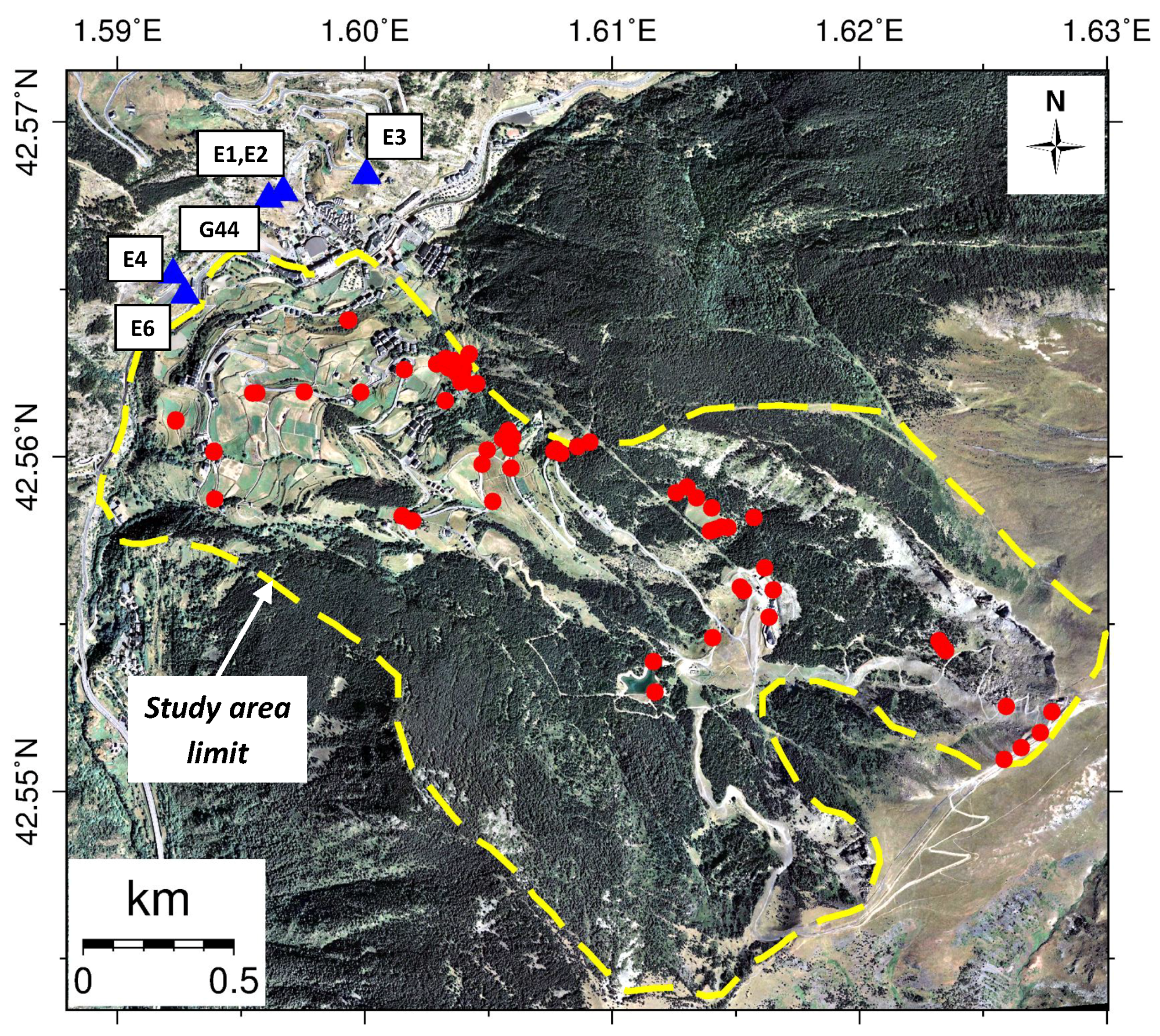
2.3. GPS Validation Data

The Canillo landslide is monitored with the Global Positioning System (GNSS/GPS) since December 2012. Although several continuous monitoring GPS techniques exist [8], the small rate of displacements justified a discontinuous approach, with yearly field campaigns [7]. A network of 78 GPS points were established at Canillo, covering most of the landslide and the surrounding area as Figure 3 shows. Six points (blue filled triangles in Figure 3) serve as base points to check the stability of the local datum. Once per year, in October, a two day campaign is carried out covering all the control points, spread along the landslide. The GPS method has been the Real Time Kinematic (RTK), with two geodetic-level receivers (Topcon Hiper-Pro, double frequency, double constellation, (Topcon Positioning Systems Inc., Tokyo, Japan)). The final results are the point coordinates in the ETRS89 reference system (Longitude, Latitude and elevation for instance). The estimated accuracy of the resulting coordinate increments is around 1 cm in planimetry and 2 cm in elevation [7].

Three GPS campaigns fit within the study period: October 2014, October 2015 and October 2016. The six base points (E1, E2, E3, E4, E6 and G44 in Figure 3), which are on the assumed stable substrate outside the unstable area, and a total of 72 control points spread over the landslide deposits have been measured. The base points were measured in order to rule out systematic or instrumental errors and thus validate the measures carried out. The control points have been distributed throughout the landslide with the aim of providing a comprehensive overview of its behavior.

The results of the displacement observed at the reference points (points E and G44 in Figure 3), outside the landslide, are within the range of the error and therefore can be considered stable, as expected. Among the 72 GPS control points within the study area limit, 37 are selected for PSI results’ validation. The correspondence between GPS points and the PSs has been made with proximity criteria but also discarding any change of geomorphological sub-unit. The difference between GPS and PSI in terms of precision, spatial resolution and temporal resolution is noticeable, but the measured displacement of these selected GPS control points can be used to examine the reliability of the PSI derived ground displacement, as it will be done in Section 4.2.

3. Methodology

In this section, the different PSI strategies that will be compared in this paper are introduced. Most of the processing steps are identical for all of them, so the description will be focused on the different PS identification methods used that characterize each strategy.

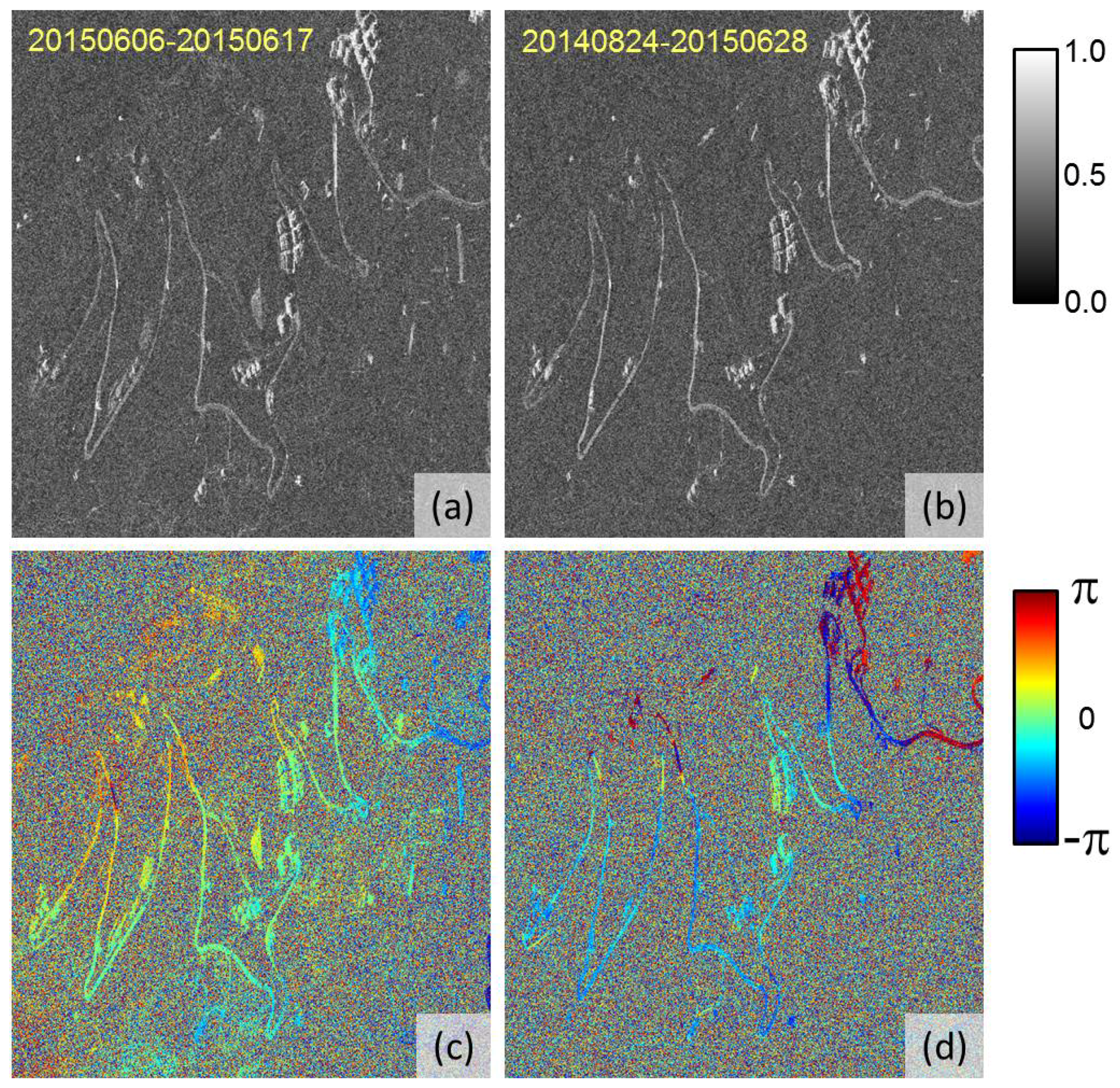
3.1. Differential SAR Interferometry (DInSAR) Processing

In the conventional strip-map mode, SAR images’ azimuth resolution is around half of the azimuth antenna length, which cannot be reduced arbitrarily to improve the resolution without the risk of causing range ambiguities. To overcome this limitation and achieve a higher resolution, the spotlight mode extends the illuminating time of each scatterer by sweeping the azimuth beam backward during imaging [46]. This brings a systematic Doppler centroid drift in the azimuth direction of the focused SAR images.

Prior to the DInSAR processing of the data, the particularities of Staring Spotlight acquisition mode have to be considered during the classical interferometric processing. When performing the image co-registration and common band filtering (if required), all base-banding steps have to consider the azimuth variation of the Doppler spectrum, which is different to the one of the stripmap mode and would require a deramping of the images involved. The details of how to deal with this issue can be found in [37,46]. The other steps of InSAR processing are identical to those of the stripmap case. The spotlight DInSAR processing module, able to work with sliding and staring data, has been implemented in the SUBSOFT-GUI, which is the UPC’s DInSAR processing chain based on the Coherent Pixel Technique (CPT) [17,20].

In this study, in order to limit the influence of geometrical and temporal decorrelation on interferograms, we set the interferograms’ temporal and spatial baseline thresholds as 365 days and 230 m, respectively. These values have allowed a good interconnection of the images and they act as upper-limits to avoid having interferograms with too long temporal or spatial baselines. The interferograms have been selected using a Delauney triangulation over the SLCs’ distribution considering its acquisition time and spatial baselines with respect a master image, as shown in Figure 4. With these restrictions and with the help of an external DEM of the area with 5 m resolution provided by the Government of Andorra, a total of 80 differential interferograms have been generated from the 32 TSX images.

One of the characteristics of X-band data is that it decorrelates very fast in vegetated areas, but, at the same time, the coherent pixels are able to preserve their phase quality very well over time. In other words, if they are coherent, they keep the coherence well. The main advantage of working with high resolution data is the capability to detect small coherent features embedded in uncorrelated areas. In order to illustrate this, Figure 5 shows two coherence maps obtained from two different interferograms using a multi-look of 5 × 3 (azimuth × range). The resolution of the multi-looked interferogram is 1.15 × 1.77 m. One with a temporal baseline of 11 days and the other with 10 months. The coherence maps look very similar for both cases demonstrating the previous statement.

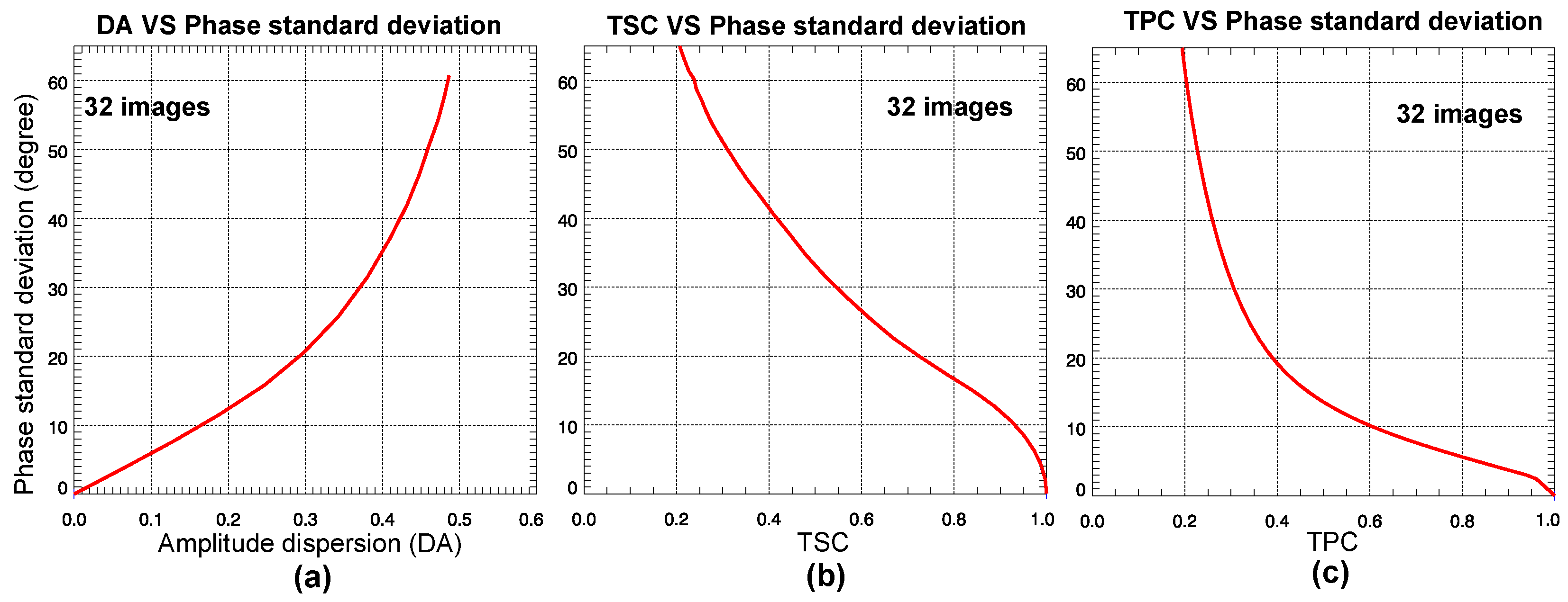
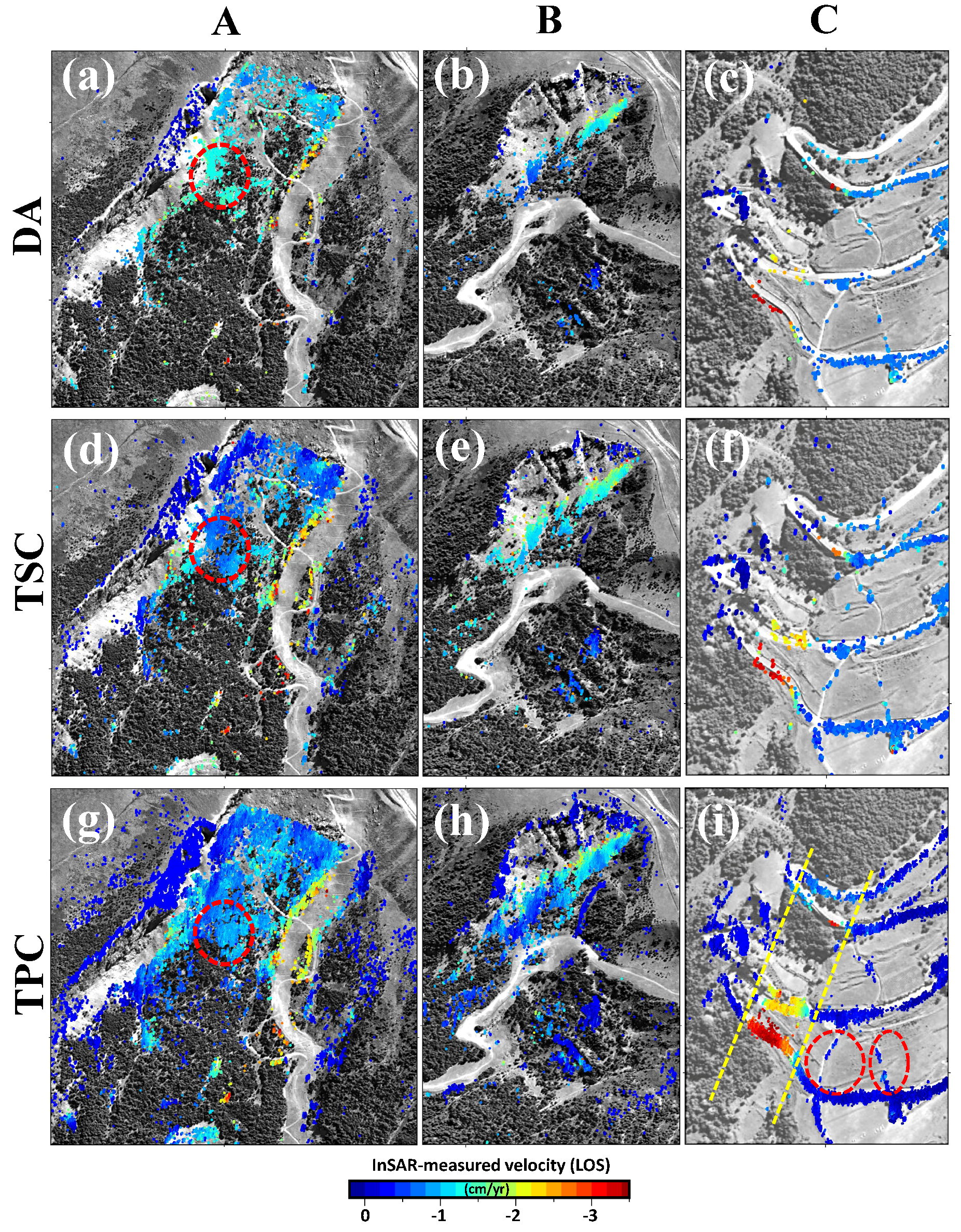
3.2. Persistent Scatterers Identification

Together with the classical full-resolution pixel selection method (i.e., the amplitude dispersion ($D_A$) method), another two techniques (the temporal sublook coherence (TSC) and the temporal phase coherence (TPC) methods) have been used to identify pixels with high phase quality, known as PS Candidates (PSCs). As the $D_A$ approach [14] is very well known by the PSI community, we will only introduce briefly the TSC and TPC approaches, which are two pixel selection methods developed by the authors.

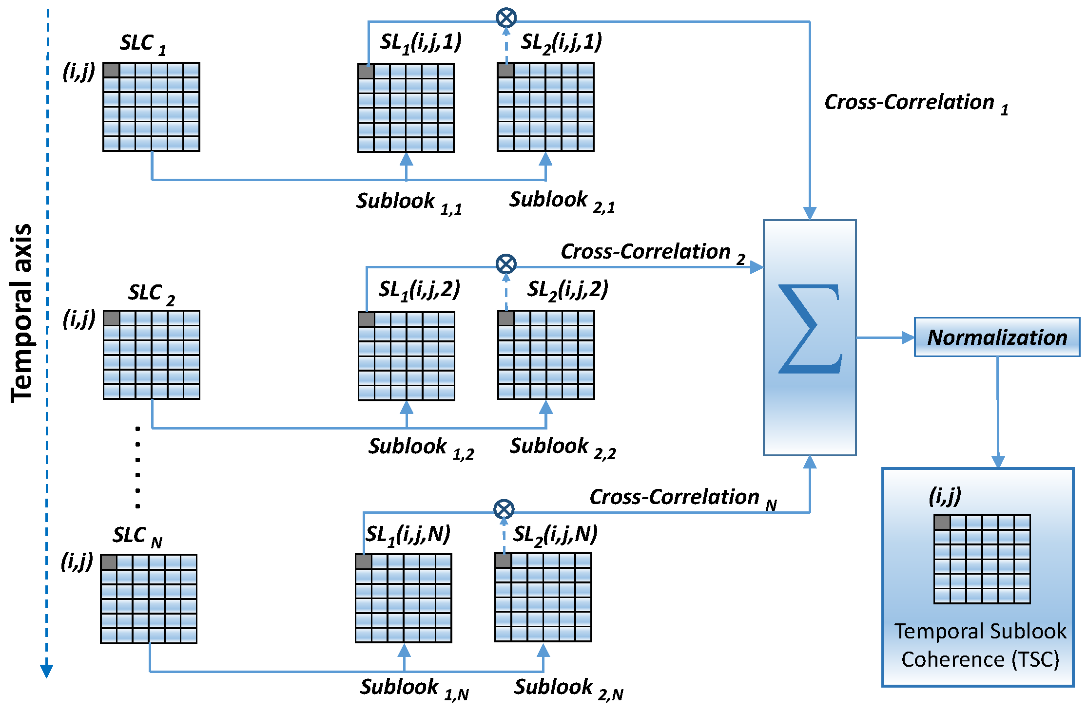
3.2.1. PS Candidates Selection by Temporal Sublook Coherence (TSC)

Different from the $D_A$ method, which selects persistent PSs by exploring pixels’ amplitude stability, the TSC method intends to identify those pixels that behave like point scatterers in the spectral domain along time [36]. Any target that presents a correlated spectrum in range, azimuth and elevation along time would be identified as PS. In practice, targets usually present a nonuniform azimuth scattering pattern, worsened in the Staring Spotlight case due to the length of the synthetic aperture, and the assumption of correlated spectrum can only be applied in range. This method presents some advantages. For instance, with this approach, the radiometric calibration of the images is not necessary since amplitude plays no role in the detection and, thus, point-like scatterers that change its amplitude along time can be perfectly selected. An example of the latter case will be highly directive targets whose reflectivity has a strong dependence on the incidence angle. In addition, it was demonstrated in [36] that it is more reliable with reduced sets of images than $D_A$.

Before TSC estimation, two range sublooks (SL) of each SAR image have to be generated. Focused SAR images are usually tapered with a linear window (Hamming, Hanning, Kaiser, etc.) to reduce the impact of the sidelobes. In order to ensure that the two sublooks in which the spectrum will be divided present a symmetrical shape, the original spectrum has to be unweighted to flatten it. Once the range spectrum has been flattened, two sublooks are generated (each one corresponding to one half of the original spectrum) and base banded to the same central frequency to avoid any undesired linear phase term during the later spectral correlation. To reduce once again the sidelobes, each sublook is tapered with a linear window. Finally, the inverse Fourier transform is applied to get both SLs in the spatial domain. A detailed explanation of the whole process is perfectly detailed in [36]. Once the sublooks of all SAR images are obtained, the TSC of any arbitrary pixel (i, j) can be calculated with Equation (1)

$$\left|{\widehat{\gamma }}_{tmp}(i,j)\right|=\frac{\left|{\displaystyle \sum _{n=1}^{N_{im}}}{S}_1(i,j,n)·S_2^{*}(i,j,n)\right|}{{\displaystyle \sum _{n=1}^{N_{im}}}{\left|S_1(i,j,n)\right|}^2·{\displaystyle \sum _{n=1}^{N_{im}}}{\left|S_2(i,j,n)\right|}^2},$$

(1)

where $S_1$ and $S_2$ are the pixel (i, j) corresponding complex values of the first and second sublook for the acquisition image n, and $N_{im}$ refers to the total number of images. The sketch of the TSC estimation for a generic pixel can be represented by Figure 6.

The temporal sublook coherence (TSC) can be regarded as the classical coherence and, similarly, pixels can be selected based on the application of a threshold. High values of TSC would be associated with point-like scatterers. Similarly to the case of classical coherence, relations between the true TSC and the expected one can be established as a function of the number of images employed, as well as the true TSC and the pixel phase standard deviation [36,37]. These relations help to perform the pixel selection based on a phase standard deviation threshold, allowing for using a criterion independent on the number of images. From the phase standard deviation, the corresponding TPC threshold can be calculated. The selected pixels can then be treated as PSs and processed by the DInSAR algorithm to derive the displacement maps and time-series.

3.2.2. PS Candidates Selection by Temporal Phase Coherence (TPC)

After removing the topographic term using an external DEM, the phase of a differential interferogram can be expressed as Equation (2)

$$\psi ={\psi }_{def}+{\psi }_{atm}+{\psi }_{orb}+{\psi }_{{\xi }_{DEM}}+{\psi }_{noise},$$

(2)

where ${\psi }_{def}$, ${\psi }_{atm}$ and ${\psi }_{orb}$ denote the phase terms introduced by displacement along the LOS direction, atmospheric artifacts (atmospheric phase screen, APS) and SAR satellite orbit indeterminations. ${\psi }_{{\xi }_{DEM}}$ is the residual phase due to the DEM error, and ${\psi }_{noise}$ is the noise phase term. This latter term can be assumed to present a random behaviour in the neighbourhood of a given pixel while the other can be assumed to be deterministic. Thus, the noise phase term can be used as a metric of pixel’s phase quality. The temporal phase coherence (TPC) can be used to evaluate the quality of a pixel from the behaviour of this phase noise along the stack of interferograms. TPC can be estimated based on ${\psi }_{noise}$ from all generated interferograms, as Equation (3) shows

$${\gamma }_{{}_{TPC}}=\frac{1}{M}·\mid \sum _{i=1}^M{e}^{j·{\psi }_{noise,i}}\mid ,$$

(3)

where M is the number of interferograms and ${\psi }_{noise,i}$ is the noise phase term of the ith interferogram.

To obtain for each interferogram the noise phase term of a pixel, it is necessary to estimate the deterministic terms. In order to do that, the neighbouring pixels will be used assuming, in theory, a spatial low-pass behaviour of all deterministic terms in the vicinity of the pixel whose TPC is being estimated, a.k.a the central pixel. The phase of the neighbouring pixels is estimated by averaging their complex values, but excluding the central pixel, and then calculating the argument of this complex number. With this approach, similarly to the classical multi-looking in interferometry, the pixels’ amplitude is used to give more significance to those pixels with higher amplitude in front of those with lower values that, in principle, can be expected to be noisier and less reliable. The first three terms of Equation (2) can be assumed to be spatially low-pass. Indeed, APS, orbital residues and the phase offset of the interferogram perfectly fulfill this condition while, for the deformation, it would be an acceptable approximation. Then, subtracting the neighbouring phase from the central phase gives Equation (4)

$${\psi }^{central}-{\psi }^{neigh}\equiv {\psi }^{dif}={\psi }_{{\xi }_{DEM}}^{dif}+{\psi }_{noise}^{dif},$$

(4)

where ${\psi }_{{\xi }_{DEM}}^{dif}={\psi }_{{\xi }_{DEM}}^{central}-{\psi }_{{\xi }_{DEM}}^{neigh}$ and ${\psi }_{noise}^{dif}={\psi }_{noise}^{central}-{\psi }_{noise}^{neigh}$. Thus, the terms have been grouped in deterministic along the interferometric stack, ${\psi }_{{\xi }_{DEM}}^{dif}$, and random, ${\psi }_{noise}^{dif}$. As (4) shows, the estimation of the noise phase of the central pixel, i.e., ${\psi }_{noise}^{central}$, would be affected by the deterministic terms. The averaging would reduce the noise term of the neighbouring pixels, ${\psi }_{noise}^{neigh}$. Thus, we can assume than ${\psi }_{noise}^{central}\approx {\psi }_{noise}^{dif}$. Thus, by subtracting the deterministic term ${\psi }_{{\xi }_{DEM}}^{dif}$ from ${\psi }^{dif}$, the noise phase of the central pixel can be estimated. In the practical implementation, all phase operations are obviously done in the complex domain.

The phases due to DEM errors (${\epsilon }_{DEM}^{central}$ and ${\epsilon }_{DEM}^{neigh}$) of the central and neighboring pixels can be rewritten as Equations (5) and (6), respectively:

$${\psi }_{{\xi }_{DEM}}^{central}=\frac{4\pi }{\lambda }·\frac{B_n}{R_0·sin\left({\vartheta }_0\right)}·{\epsilon }_{DEM}^{central},$$

(5)

$${\psi }_{{\xi }_{DEM}}^{neigh}=\frac{4\pi }{\lambda }·\frac{B_n}{R_0·sin\left({\vartheta }_0\right)}·{\epsilon }_{DEM}^{neigh},$$

(6)

where $\lambda , B_n, R_0$ and ${\vartheta }_0$ are the wavelength, the perpendicular baseline, the absolute range distance in the LOS direction between the sensor and the target and the incidence angle, respectively. Then, we can derive ${\psi }_{{\xi }_{DEM}}^{dif}$ as (7)

$${\psi }_{{\xi }_{DEM}}^{dif}=\frac{4\pi }{\lambda }·\frac{B_n}{R_0·sin\left({\vartheta }_0\right)}·△{\epsilon }_{DEM},$$

(7)

where $△{\epsilon }_{DEM}={\epsilon }_{DEM}^{central}-{\epsilon }_{DEM}^{neigh}$ is the difference of DEM errors between the central and the averaged error of the neighboring pixels. We use Equation (8) to estimate each pixel’s $△{\epsilon }_{DEM}$ and then the ${\psi }_{{\xi }_{DEM}}^{dif}$ is calculated by Equation (7):

$$arg\underset{△{\epsilon }_{DEM}}{max}\{{\gamma }_{{}_{TPC}}=\frac{1}{M}·\mid \sum _{i=1}^M{e}^{j·{\psi }_i^{dif}-j·{\psi }_{{\xi }_{DEM},i}^{dif}}\mid \}.$$

(8)

Until now, ${\psi }_{{\xi }_{DEM}}^{dif}$ has been estimated and then ${\psi }_{noise}^{central}$ can be derived by Equation (4) under the assumption that ${\psi }_{noise}^{central}\approx {\psi }_{noise}^{dif}$. All pixels’ noise phase terms of all the interferograms can be estimated by this way and then the TPC can be calculated by Equation (3).

TPC provides a temporal coherence of each pixel and fixing a threshold can perform the identification of PSCs. As in the case of classical coherence or the TSC, a relationship between TPC and the phase standard can be established in order to select a threshold independent on the number of images and interferograms. The derivation of these relations has been discussed in detail in [38].

3.3. Linear and Nonlinear (Time-Series) Displacement Estimation

The linear and nonlinear displacement terms and the DEM error can be estimated by using UPC’s ground motion detection software SUBSOFT-GUI (UPC, Barcelona, Spain). SUBSOFT-GUI is a user-friendly software package for PSI processing. It allows for performing all required steps, starting from the image co-registration, differential interferograms generation and filtering, pixel selection and deformation time-series extraction. The software uses a Graphical User Interface (GUI) and most of the steps have been automatized, which facilitates the processing of any dataset. The detailed procedures of the linear and nonlinear blocks in SUBSOFT-GUI can be found by referring to [17,20]. Three independent processes, based on the same set of differential interferograms but with three different PS selection strategies ($D_A$, TSC and TPC approaches), have been carried out to compare the performance of each pixel selection technique under similar conditions. For each strategy, the measured parameter can be related with a phase standard deviation as shown in Figure 7.

The comparison of the different strategies is always a difficult task as there are many parameters that can be adjusted. In this case, the key point that makes the difference is the capability of the different strategies to select PSs. The larger the number, the better performance of the PSI processing, as it allows a better connection of the different areas and reduces the chances of having isolated clusters of PSs. It is also true that the three processes could have been optimized with a fine-tuning of the processing parameters, but, in practice, it is expected that the possible small variations on the final results would not be enough to modify the conclusions.

3.4. Atmospheric Artefacts

InSAR observations are usually plagued by propagation delays, which are also known as atmosphere phase screen (APS). As the atmosphere properties (temperature, pressure, and relative humidity that set the refractive index) between radar platform and the ground targets vary spatially and temporally, the phase delays vary from one day to another. For microwaves, it is well known that propagation delays have two major sources: tropospheric terms and ionosphere effects. At X-band, ionosphere is almost invisible and so the only significant source is the troposphere [26,47]. The atmospheric propagation delay in interferograms can be categorized into vertical stratification and turbulence mixing [26]. While the latter can be compensated, thanks to its random behaviour in time and correlated behaviour in space, with a set of temporal and spatial filters during data processing [14,18,20], the former can be much more difficult. Stratification is prone to occurring in areas with steep topography and the APS appears to be strongly correlated with the elevation. If not properly compensated, APS can be misinterpreted as topography or displacement. Different strategies can be used to characterize and compensate the stratified APS, for instance with models following a linear or quadratic phase-elevation relationship [25,27,28,29].

The time of the pass of the satellite for the TSX data acquisitions was early in the morning, around 6:03 a.m. UTC (8:03 a.m. in local summer time and 7:03 a.m. in local winter time). At this time of the day, the atmosphere is very stable, compared with the strong fluctuations that can be observed during the day, and stratified APS has not been observed in the dataset.

4. Results and Discussion

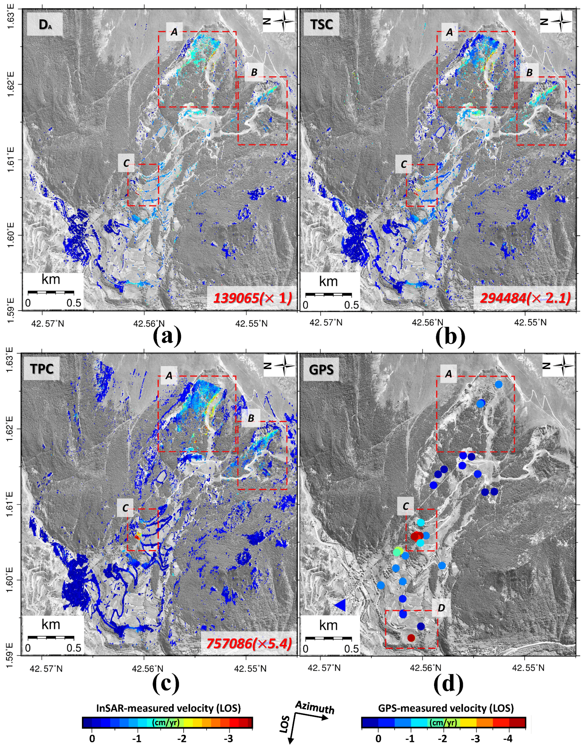
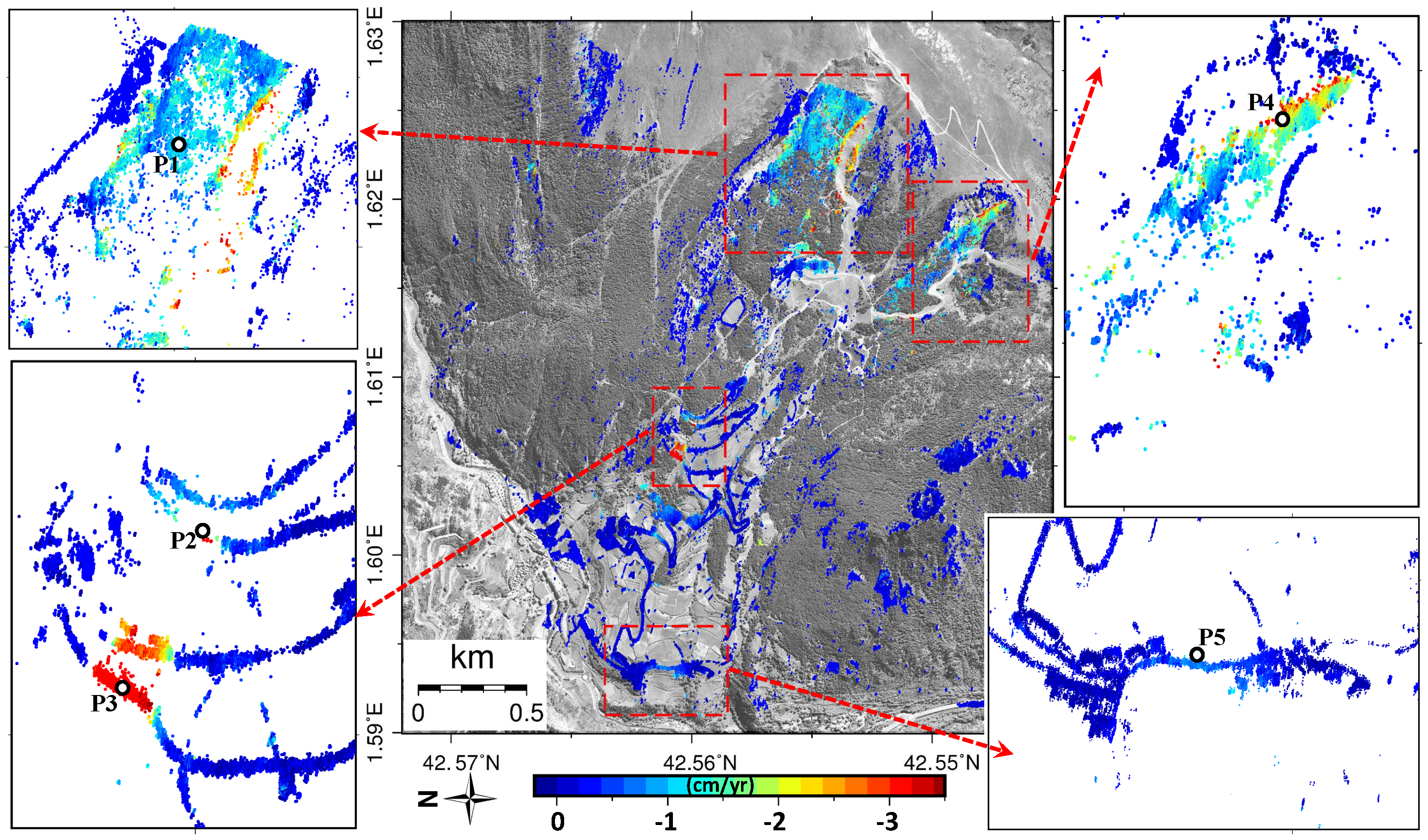
4.1. Line-of-Sight (LOS) Monitoring Results

The LOS displacement rate maps derived by the three methods (i.e., the $D_A$, TSC and TPC) are shown in Figure 8a–c, respectively. To make a fair comparison, the pixel selection thresholds for all the three methods were established based on a phase standard deviation of $15°$. Using the plots shown in Figure 7, the corresponding thresholds for each strategy can be selected. Similar displacement trends have been detected by all of them, and the maximum displacement velocity reaches up to −3.5 cm/year (the minus sign means movement away from the satellite, i.e., downslope motion due to the landslide orientation). Within the landslide limits, there are mainly three large displacement subareas (indicated by the red rectangles in Figure 8a–c), located at the El Pic de Maians (subarea A), costa de les Gerqueres (subarea B) and Cal Borró-Cal Ponet (subarea C), respectively. These three subareas’ locations and displacement patterns are coincident with the monitoring results obtained with another dataset in 2011 [37]. The dataset consisted on Sliding-spotlight TerraSAR and GB-SAR images, and data from inclinometers deployed in the landslide, all acquired from October 2010 until October 2011. Previous results have confirmed that the location and evolution of the landslide body have not changed significantly during the recent years. This fact is in good agreement with the geological expectations.

Among the three pixel selection methods, $D_A$ and TSC select pixels that behave as point scatterers while TPC can work on both point and distributed scatterers (DSs). Since there are many DS pixels (e.g., the road) in the study area, TPC obtains a much higher density of measurement pixels (MP) than $D_A$ and TSC approaches.

Notice in Figure 8 how well the TPC method has identified those pixels along the downhill road, while the other two have just selected a reduced set of them. At the same time, the TSC method obtains more PSs than $D_A$. This can be explained by the fact that the $D_A$ method is very sensitive to the amplitude changes that highly directive scatterers produce when the local incidence angle changes from image to image. Specifically, the number of PSs obtained by TPC method is 757,086, the counterparts of TSC and $D_A$ methods are 139,065 and 294,484, respectively. The improvement of the TPC and TSC methods on $D_A$ is around ×5.4 and ×2.1, respectively. The TPC method thus has the best performance in terms of PSs’ density.

To better analyse the details of the landslide, the three subareas’ monitoring results have been enlarged and plotted in Figure 9. From column A (results of the subarea A), we can find that the displacement velocities obtained by $D_A$ (−1.3 cm/yr) are greater then those of TSC and TPC (−0.6 cm/yr) at the locations highlighted by the red ellipses. Similar differences can be observed between the TPC derived results and the other two methods within the subarea C (along the downhill road). These displacement velocities’ differences are mainly caused by the sparsity of selected pixels that reduces the number of connections of $D_A$ (Figure 9a,c) or TSC (Figure 9f) during the linear displacement estimation. Different areas interconnected by low-quality links can lead to small offsets in the velocity results. The sparser the local connections, the more easily the estimated displacement can be affected by nearby lower quality pixels and APS. Therefore, the high estimated displacement velocities in Figure 9a,c,f are mostly due to the low densities of PSs within these local areas.

As Figure 9g–i shows, thanks to the super high resolution (SHR) of the images and TPC’s good performance on pixel selection, the displacement details of the different landslide units are well detected. For instance, more pixels have been selected along the narrow paths (around 1 m in width), as highlighted by red ellipses in Figure 9i. Benefiting from this high density of PSs, the displacement boundaries (illustrated by the yellow dashed lines in Figure 9i) can be clearly determined by the TPC approach in subarea C. These boundaries can hardly be seen from the results of the other two methods, as shown in Figure 9c,f.

Besides the displacement results, PSI techniques can also obtain the DEM error of the selected pixels with respect to the reference DEM used. The inclusion of the retrieved DEM error on the geocoding of the final results largely improves the geolocation quality of the displacement maps. Figure 10 shows some interesting examples that illustrate the capabilities of SHR TSX data to retrieve the vertical distribution of scatterers in manmade structures. The examples shown have been obtained from the TPC processing. Figure 10a shows a communications tower located in Canillo. The vertical distribution of scatterers perfectly follows the tower’s structure as the picture validates. It is also interesting, looking at the GoogleEarth image, to compare the distribution of scatterers with the shadow of the tower projected over ground. Figure 10b and c show a couple of chairlifts from the Grandvalira ski station. Once again, the vertical distribution of scatterers perfectly follows the metallic structure, as the pictures and projected shadows demonstrate. Finally, Figure 10d shows a couple of high voltage towers. The good performance of the vertical location of the scatterers, thanks to the inclusion of the calculated DEM error on the geocoding process, can also be used as proof of the reliability of the displacement velocity maps obtained. Both velocity and DEM error have been calculated simultaneously when adjusting the linear model to the interferometric data [17,20].

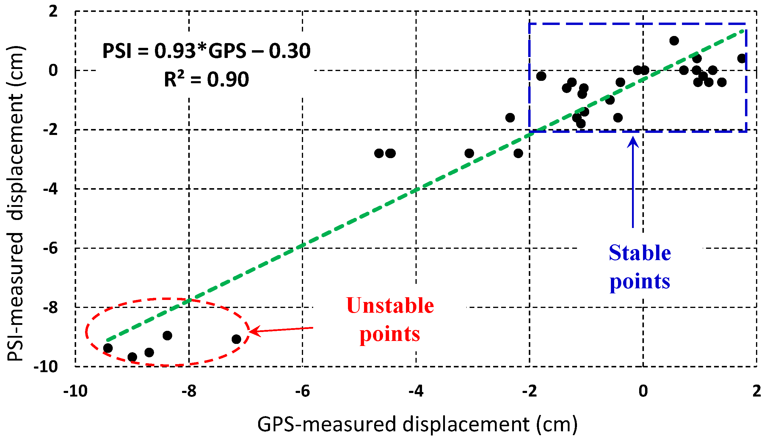
4.2. Comparison with GPS Measurements

The displacement velocities of the 37 GPS control points introduced in Section 2.3 have been projected to the LOS direction [48,49] to compare them with the DInSAR results, as shown in Figure 8d. In subarea A of Figure 8d, a small displacement with a velocity around −1 cm/yr has been detected. In the subarea C, significant movement with velocity around −4 cm/yr has been monitored by the GPS. In the subareas A and C, the GPS and PSI measured displacement velocities are consistent with each other. Unfortunately, no GPS points were available in the subarea B for comparison. On the contrary, large displacements have been recorded by the GPS within the subarea D (highlighted by the red rectangle in Figure 8d), where there are no counterpart PSI pixels in its near vicinity. However, the further neighboring PSI pixels present LOS velocities about −1.5 cm/yr, providing evidence of the agreement of the GPS and PSI results also in this subarea.

To summarize the comparison, a scatter plot with the GPS and PSI derived displacements is shown in Figure 11. In this plot, the PSI displacements are estimated by averaging those of the neighbouring pixels of the related GPS measurement point (less than 50 m apart). In addition, they have been determined from the displacement time-series taking the overall two year displacement from October 2014 to October 2016, as the GPS date campaigns. As Figure 11 reveals, the GPS and PSI displacements follow the same trends and present a correlation coefficient of $R^2$ = 0.90. For GPS measurement points with noticeable displacement (highlighted by the red ellipse in Figure 11), their surrounding PSI pixels show large displacements as well. Meanwhile, for those stable GPS measurement points (limited by the blue rectangle), with displacements between −2 to 2 cm, their corresponding PSI displacements are also within this range.

4.3. Down-Slope (DSL) Direction Displacement Monitoring Result

The ground motion derived by DInSAR is along the LOS direction, but it is usually projected to the down-slope (DSL) direction to better interpret the landslide displacement. The detailed LOS to DSL direction projection method can be found by referring to [12,24]. As it is out the scope of this paper, we do not describe it here. We projected the TPC method’s ground displacement velocities to the DSL direction, and the result is shown by Figure 12. It has to be noted that, when doing the projection, only those PSs with projection factors smaller than 3 have been preserved to avoid artificially amplifying displacement values and noise when the slope is gentle. Thanks to the relative orientation of the landslide with respect the satellite path, most of the projection factors within this study area are small. Thus, the majority of PSs have been preserved, and the displacement patterns along the LOS and DSL directions are similar (e.g., the neighboring area of P1). Except for a small set of pixels nearby point P4 in Figure 12, the displacement velocities of the previous three displacement subareas (in Figure 8c) have not been heavily amplified via the projection.

Besides the subareas A, B and C in Figure 8, in Figure 12, we have highlighted another subarea, which is located at the foot of the hill. In this subarea, noticeable displacement has been identified at the location of P5, which may be caused by the extrusion of the landslide main body moving towards the downhill direction.

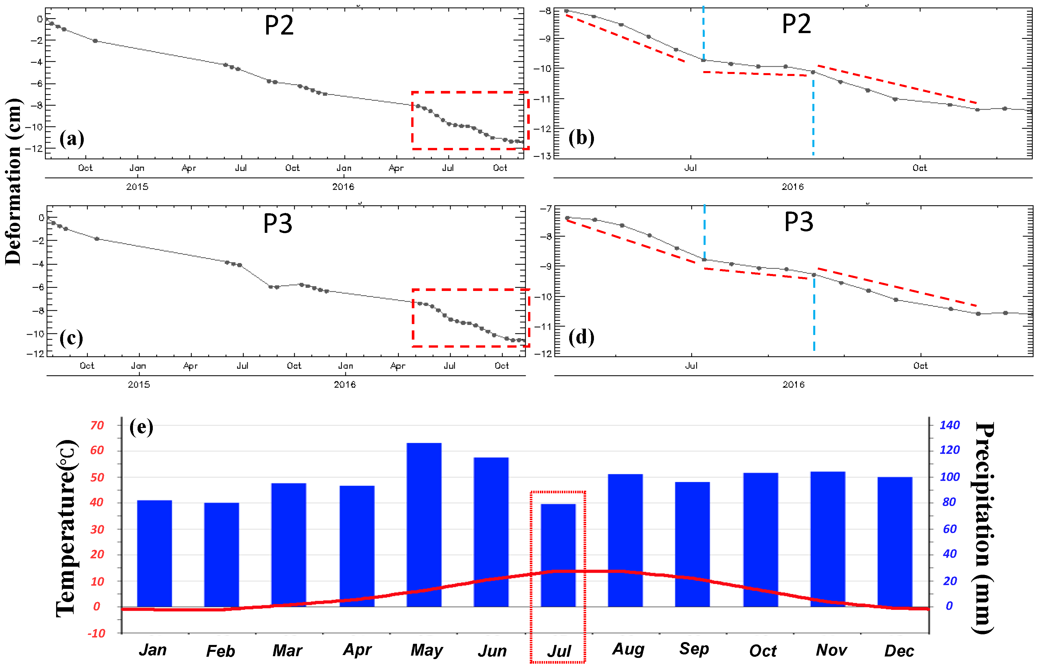
4.4. PSI Time-Series

To investigate the temporal evolution of the Canillo landslide, the DSL time-series displacement results obtained by the TPC method at two different PSs (P2 and P3 in Figure 12) have been plotted in Figure 13. The displacements observed for both PSs are exhibiting considerable nonlinear components, presenting some acceleration and deceleration periods within each year. From the two PSs’ 2016 displacement time-series (Figure 13b,d), we can find that the stable periods start at the beginning of July and end at the middle of August. These periods are coincident with the trend of Canillo averaged monthly precipitation, where the lowest precipitation is in July with an average of 79 mm, as Figure 13e shows. This indicates that the movements of the landslide have some seasonal patterns, which are correlated with the amount of precipitation.

5. Comparison with Low-Resolution Data

Sentinel-1A data of the study area have been processed with $D_A$ and TPC methods to highlight the advantages of the SHR data in regional-scale landslide monitoring. TSC has not been included as it provides similar results than TPC. Sentinel-1A images have resolutions of 14 and 2.5 m in azimuth and range directions, respectively. Fourteen Sentinel-1A SAR images acquired from the 11 May 2016 to 19 November 2016 have been employed to generate 33 interferograms. In the pixel selection step, the same phase standard deviation threshold ($15°$) as with TSX data has been used. The displacement velocity maps obtained using the two PSI strategies, $D_A$ and TPC, are shown in Figure 14.

Similarly to the case of TSX data, TPC is able to obtain much more PSs than $D_A$ (×4.0), and the displacement trends derived are similar to those of TSX but less detailed. For both methods, their PSs’ densities have decreased dramatically compared with the TSX data case. Specifically, for $D_A$ and TPC methods, the numbers of PSs are ×146 and ×197 less w.r.t. that of the TSX case. This significant reduction of the PSs’ density is mainly due to two reasons that are closely related. In addition to the logical reduction due to the coarse resolution of Sentinel-1A data, there is also the fact that many small PSs surrounded by decorrelated pixels that were detected with SHR data are now mixed all together due to the worse resolution and, consequently, not detected.

The Sentinel-1A data monitoring results of the Cal Borró-Cal Ponet section (subarea C in Figure 8 and where the strongest displacement has been detected) have been highlighted with a red rectangle in Figure 14. In this subsection, the displacement clearly detected with TSX data does not appear in the Sentinel-1A results with none of the pixel selection methods. A detailed view of Cal Borró is shown in Figure 15. Similarly, Figure 14 shows no noticeable displacement in any of the other two subareas (subareas A and B in Figure 8c). However, the small displacement at the base of the landslide is detected with both PSI strategies and agrees with the results of SHR data. Moreover, the sparse distribution of PSs, which can be poorly interconnected, allows the appearance of some outliers, pixels whose velocities are clearly erroneous, scattered along the image. The presence of outliers is more noticeable on the $D_A$ results in the form of isolated red points, those with the highest velocities.

To conclude, for regional-scale landslide monitoring, the TSX SHR SAR images have the advantage of obtaining more detailed monitoring results with better reliability compared with those of lower resolution sensors.

6. Conclusions

In this paper, the ability of super high-spatial resolution (SHR) SAR images together with advanced PS selection strategies for regional-scale landslide monitoring in a challenging area has been studied. Thirty-two SHR TerraSAR-X (TSX) images (July 2014 to October 2016), with resolutions of 0.23 and 0.59 m in azimuth and range directions, have been employed to monitor the Canillo landslide (Andorra) by using PSI techniques with three different pixel selection methods.

This study has demonstrated that improving the number of high-quality pixels for its later PSI processing results of crucial importance in landslide monitoring in natural environments. Under the application point of view, to the authors’ knowledge, it is one of the first times when such a high density of PS has been obtained in mountainous areas. SHR SAR data jointly with advanced full-resolution PSI strategies allow the achievement of a more robust network of PS (improving the linear estimation without propagation errors and the reliable estimation of APS) and thus favors the reliable estimation of displacement maps in a major number of points inside a landslide. This is a general conclusion that does not depend on the landslide. A different issue is if the particularities of a given landslide (orientation, type of vegetation coverage, local topography, snow episodes, etc.) made it unsuitable for PSI monitoring. Similarly, well-established interferometric techniques for DEM generation fail on forested areas. It is clear that the particular characteristics of the scenario may limit the application of the technique.

The landslide’s overall displacement patterns observed by the three methods in El Forn de Canillo are similar. Three main subareas with noticeable displacement have been detected, which are similar to those obtained in previous PSI monitoring results. This indicates that the evolution of the landslide main body did not change significantly during recent years. The PSI measured displacement rates have been compared with GPS measurements of the same period, and they are both in good agreement. It is worth highlighting the higher information/resolution of the PSI techniques in comparison with the GPS low point density, as it can be appreciated in Figure 8. Although already highlighted in the literature, in the Canillo Landslide, the PSI capability for detecting incipient movements in zones not previously surveyed by the geological engineering specialists has been verified (as the subarea costa de les Gerqueres, red rectangle B in Figure 8).The displacement time-series of two significant pixels are characterized by considerable nonlinear components, exhibiting some acceleration and stabilization periods within each year. These periods can be correlated with the averaged monthly precipitation amounts, revealing the important influence of rain/snow melting episodes on the development of this landslide.

SHR SAR data initially designed for improving monitoring capabilities over man-made structures, such as buildings, bridges, railways or highways, have also demonstrated an outstanding performance over natural reflectors, such as outcrops or exposed rocks with the proper PSs selection strategy. Indeed, this improvement in terms of density allows a better characterization and delineation of complex landslides. Among the three full-resolution PSC selection strategies, the advanced ones (i.e., the TSC and TPC) are able to obtain much more valid PSs than the classical $D_A$ method. The TPC method presents the best performance. Thanks to these huge amount of PSs, the displacement details of the regional-scale landslides can be characterized with better precision when combining the TPC method with SHR TSX data. Compared with the lower-spatial resolution SAR data (Sentinel-1A in this study), SHR data can better characterize the landslide, particularly if the different subareas are small.

The results of this work show that the density of valid PSs can be greatly enhanced by using the TPC method together with SHR SAR images. Thus, they can together be used as a powerful tool for detailed landslide monitoring in difficult areas.

References

1. Dunnicliff, J.; Green, G.E. Geotechnical Instrumentation for Monitoring Field Performance; John Wiley & Sons: Hoboken, NJ, USA, 1993. [Google Scholar]
2. Pinyol, N.M.; Alonso, E.E.; Corominas, J.; Moya, J. Canelles landslide: Modelling rapid drawdown and fast potential sliding. Landslides 2012, 9, 33–51. [Google Scholar] [CrossRef]
3. Ramesh, M.V. Design, development, and deployment of a wireless sensor network for detection of landslides. Ad Hoc Netw. 2014, 13, 2–18. [Google Scholar] [CrossRef]
4. Uhlemann, S.; Smith, A.; Chambers, J.; Dixon, N.; Dijkstra, T.; Haslam, E.; Meldrum, P.; Merritt, A.; Gunn, D.; Mackay, J. Assessment of ground-based monitoring techniques applied to landslide investigations. Geomorphology 2016, 253, 438–451. [Google Scholar] [CrossRef] [Green Version]
5. Zhang, Y.; Tang, H.; Li, C.; Lu, G.; Cai, Y.; Zhang, J.; Tan, F. Design and Testing of a Flexible Inclinometer Probe for Model Tests of Landslide Deep Displacement Measurement. Sensors 2018, 18, 224. [Google Scholar] [CrossRef] [PubMed]
6. Calcaterra, S.; Cesi, C.; Di Maio, C.; Gambino, P.; Merli, K.; Vallario, M.; Vassallo, R. Surface displacements of two landslides evaluated by GPS and inclinometer systems: A case study in Southern Apennines, Italy. Nat. Hazards 2012, 61, 257–266. [Google Scholar] [CrossRef]
7. Gili, J.A.; Corominas, J.; Rius, J. Using Global Positioning System techniques in landslide monitoring. Eng. Geol. 2000, 55, 167–192. [Google Scholar] [CrossRef]
8. Malet, J.P.; Maquaire, O.; Calais, E. The use of Global Positioning System techniques for the continuous monitoring of landslides: Application to the Super-Sauze earthflow (Alpes-de-Haute-Provence, France). Geomorphology 2002, 43, 33–54. [Google Scholar] [CrossRef]
9. Colesanti, C.; Wasowski, J. Investigating landslides with space-borne Synthetic Aperture Radar (SAR) interferometry. Eng. Geol. 2006, 88, 173–199. [Google Scholar] [CrossRef]
10. Wasowski, J.; Bovenga, F. Investigating landslides and unstable slopes with satellite Multi Temporal Interferometry: Current issues and future perspectives. Eng. Geol. 2014, 174, 103–138. [Google Scholar] [CrossRef]
11. Bovenga, F.; Wasowski, J.; Nitti, D.; Nutricato, R.; Chiaradia, M. Using COSMO/SkyMed X-band and ENVISAT C-band SAR interferometry for landslides analysis. Remote Sens. Environ. 2012, 119, 272–285. [Google Scholar] [CrossRef]
12. Hu, X.; Wang, T.; Pierson, T.C.; Lu, Z.; Kim, J.; Cecere, T.H. Detecting seasonal landslide movement within the Cascade landslide complex (Washington) using time-series SAR imagery. Remote Sens. Environ. 2016, 187, 49–61. [Google Scholar] [CrossRef]
13. Confuorto, P.; Di Martire, D.; Centolanza, G.; Iglesias, R.; Mallorqui, J.J.; Novellino, A.; Plank, S.; Ramondini, M.; Thuro, K.; Calcaterra, D. Post-failure evolution analysis of a rainfall-triggered landslide by multi-temporal interferometry SAR approaches integrated with geotechnical analysis. Remote Sens. Environ. 2017, 188, 51–72. [Google Scholar] [CrossRef]
14. Ferretti, A.; Prati, C.; Rocca, F. Permanent scatterers in SAR interferometry. IEEE Trans. Geosci. Remote Sens. 2001, 39, 8–20. [Google Scholar] [CrossRef] [Green Version]
15. Ferretti, A.; Fumagalli, A.; Novali, F.; Prati, C.; Rocca, F.; Rucci, A. A new algorithm for processing interferometric data-stacks: SqueeSAR. IEEE Trans. Geosci. Remote Sens. 2011, 49, 3460–3470. [Google Scholar] [CrossRef]
16. Berardino, P.; Fornaro, G.; Lanari, R.; Sansosti, E. A new algorithm for surface deformation monitoring based on small baseline differential SAR interferograms. IEEE Trans. Geosci. Remote Sens. 2002, 40, 2375–2383. [Google Scholar] [CrossRef]
17. Mora, O.; Mallorqui, J.J.; Broquetas, A. Linear and nonlinear terrain deformation maps from a reduced set of interferometric SAR images. IEEE Trans. Geosci. Remote Sens. 2003, 41, 2243–2253. [Google Scholar] [CrossRef]
18. Lanari, R.; Mora, O.; Manunta, M.; Mallorquí, J.J.; Berardino, P.; Sansosti, E. A small-baseline approach for investigating deformations on full-resolution differential SAR interferograms. IEEE Tran. Geosci. Remote Sens. 2004, 42, 1377–1386. [Google Scholar] [CrossRef]
19. Hooper, A.; Zebker, H.; Segall, P.; Kampes, B. A new method for measuring deformation on volcanoes and other natural terrains using InSAR persistent scatterers. Geophys. Res. Lett. 2004, 31. [Google Scholar] [CrossRef] [Green Version]
20. Blanco-Sanchez, P.; Mallorquí, J.J.; Duque, S.; Monells, D. The coherent pixels technique (CPT): An advanced DInSAR technique for nonlinear deformation monitoring. Pure Appl. Geophys. 2008, 165, 1167–1193. [Google Scholar] [CrossRef]
21. Iglesias, R.; Monells, D.; Fabregas, X.; Mallorqui, J.J.; Aguasca, A.; Lopez-Martinez, C. Phase quality optimization in polarimetric differential SAR interferometry. IEEE Trans. Geosci. Remote Sens. 2014, 52, 2875–2888. [Google Scholar] [CrossRef]
22. Cruden, D.M.; Varnes, D.J. Landslide types and processes. In Landslides: Investigation and Mitigation; Turner, A., Schuster, R., Eds.; Transportation Research Board, US National Research Council: Washington, DC, USA, 1996; Volume 247, Chapter 3; pp. 36–75. [Google Scholar]
23. Hungr, O.; Leroueil, S.; Picarelli, L. The Varnes classification of landslide types, an update. Landslides 2014, 11, 167–194. [Google Scholar] [CrossRef]
24. Iglesias, R. High-Resolution Space-Borne and Ground-Based SAR Persistent Scatterer Interferometry for Landslide Monitoring. Ph.D. Thesis, Universitat Politècnica de Catalunya, Barcelona, Spain, 2015. [Google Scholar]
25. Beauducel, F.; Briole, P.; Froger, J.L. Volcano-wide fringes in ERS synthetic aperture radar interferograms of Etna (1992–1998): Deformation or tropospheric effect? J. Geophys. Res. Solid Earth 2000, 105, 16391–16402. [Google Scholar] [CrossRef]
26. Hanssen, R.F. Radar Interferometry: Data Interpretation and Error Analysis; Vol. 2, Springer Science & Business Media: Dordrecht, Tthe Netherlands, 2001. [Google Scholar]
27. Elliott, J.; Biggs, J.; Parsons, B.; Wright, T. InSAR slip rate determination on the Altyn Tagh Fault, northern Tibet, in the presence of topographically correlated atmospheric delays. Geophys. Res. Lett. 2008, 35. [Google Scholar] [CrossRef] [Green Version]
28. Iglesias, R.; Fabregas, X.; Aguasca, A.; Mallorqui, J.J.; López-Martínez, C.; Gili, J.A.; Corominas, J. Atmospheric phase screen compensation in ground-based SAR with a multiple-regression model over mountainous regions. IEEE Trans. Geosci. Remote Sens. 2014, 52, 2436–2449. [Google Scholar] [CrossRef]
29. Hu, Z.; Mallorquí, J.J.; Centolanza, G.; Duro, J. Insar atmospheric delays compensation: Case study in tenerife island. In Proceedings of the 2017 IEEE International Geoscience and Remote Sensing Symposium (IGARSS), Fort Worth, TX, USA, 23–28 July 2017; pp. 3167–3170. [Google Scholar]
30. Bamler, R.; Eineder, M.; Adam, N.; Zhu, X.; Gernhardt, S. Interferometric potential of high resolution spaceborne SAR. Photogramm.-Fernerkund.-Geoinf. 2009, 2009, 407–419. [Google Scholar] [CrossRef]
31. Prati, C.; Ferretti, A.; Perissin, D. Recent advances on surface ground deformation measurement by means of repeated space-borne SAR observations. J. Geodyn. 2010, 49, 161–170. [Google Scholar] [CrossRef] [Green Version]
32. Lee, J.S.; Jurkevich, L.; Dewaele, P.; Wambacq, P.; Oosterlinck, A. Speckle filtering of synthetic aperture radar images: A review. Remote Sens. Rev. 1994, 8, 313–340. [Google Scholar] [CrossRef]
33. Daba, J.S.; Jreije, P. Advanced stochastic models for partially developed speckle. World Acad. Sci. Eng. Technol. 2008, 41, 566–570. [Google Scholar]
34. Lopes, A.; Nezry, E.; Touzi, R.; Laur, H. Structure detection and statistical adaptive speckle filtering in SAR images. Int. J. Remote Sens. 1993, 14, 1735–1758. [Google Scholar] [CrossRef]
35. Curlander, J.C.; McDonough, R.N. Synthetic Aperture Radar; John Wiley & Sons: New York, NY, USA, 1991; Volume 396. [Google Scholar]
36. Iglesias, R.; Mallorqui, J.J.; López-Dekker, P. DInSAR pixel selection based on sublook spectral correlation along time. IEEE Trans. Geosci. Remote Sens. 2014, 52, 3788–3799. [Google Scholar] [CrossRef]
37. Iglesias, R.; Mallorqui, J.J.; Monells, D.; López-Martínez, C.; Fabregas, X.; Aguasca, A.; Gili, J.A.; Corominas, J. PSI deformation map retrieval by means of temporal sublook coherence on reduced sets of SAR images. Remote Sens. 2015, 7, 530–563. [Google Scholar] [CrossRef] [Green Version]
38. Zhao, F.; Mallorqui, J.J. A temporal phase coherence estimation algorithm and its application on DInSAR pixel selection. IEEE Trans. Geosci. Remote Sens. 2018. Undergoing Review. [Google Scholar]
39. Duque, S.; Breit, H.; Balss, U.; Parizzi, A. Absolute height estimation using a single TerraSAR-X staring spotlight acquisition. IEEE Geosci. Remote Sens. Lett. 2015, 12, 1735–1739. [Google Scholar] [CrossRef]
40. Tapete, D.; Cigna, F.; Donoghue, D.N. ‘Looting marks’ in space-borne SAR imagery: Measuring rates of archaeological looting in Apamea (Syria) with TerraSAR-X Staring Spotlight. Remote Sens. Environ. 2016, 178, 42–58. [Google Scholar] [CrossRef]
41. Corominas, J.; Alonso, E. Inestabilidad de Laderas en el Pirineo Catalán. Tipología y causas. In Proceedings of the Inestabilidad de laderas en el Pirineo, Barcelona, Spain, 16–17 January 1984; pp. 1–53. [Google Scholar]
42. Santacana, N. Estudi dels Grans Esllavissaments d’Andorra: Els Casos del Forn i del Vessant d’Encampadana. Master’s Thesis, Department of Dynamic Geology, Geophysics and Paleontology, Faculty of Geology, University of Barcelona, Barcelona, Spain, 1994. [Google Scholar]
43. Corominas, J.; Iglesias, R.; Aguasca, A.; Mallorquí, J.J.; Fàbregas, X.; Planas, X.; Gili, J.A. Comparing satellite based and ground based radar interferometry and field observations at the Canillo landslide (Pyrenees). In Engineering Geology for Society and Territory-Volume 2; Springer: Cham, Switzerland, 2015; pp. 333–337. [Google Scholar]
44. Torrebadella, J.; Villaró, I.; Altimir, J.; Amigó, J.; Vilaplana, J.; Corominas, J.; Planas, X. El deslizamiento del Forn de Canillo en Andorra. Un ejemplo de gestión del riesgo geológico en zonas habitadas en grandes deslizamientos. In Proceedings of the VII Simposio Nacional Sobre Taludes y Laderas Inestables, Barcelona, Spain, 27–30 October 2009; pp. 403–414. [Google Scholar]
45. Mittermayer, J.; Wollstadt, S.; Prats-Iraola, P.; Scheiber, R. The TerraSAR-X staring spotlight mode concept. IEEE Trans. Geosci. Remote Sens. 2014, 52, 3695–3706. [Google Scholar] [CrossRef]
46. Eineder, M.; Adam, N.; Bamler, R.; Yague-Martinez, N.; Breit, H. Spaceborne spotlight SAR interferometry with TerraSAR-X. IEEE Trans. Geosci. Remote Sens. 2009, 47, 1524–1535. [Google Scholar] [CrossRef]
47. Davis, J.; Herring, T.; Shapiro, I.; Rogers, A.; Elgered, G. Geodesy by radio interferometry: Effects of atmospheric modeling errors on estimates of baseline length. Radio Sci. 1985, 20, 1593–1607. [Google Scholar] [CrossRef] [Green Version]
48. Cascini, L.; Fornaro, G.; Peduto, D. Advanced low-and full-resolution DInSAR map generation for slow-moving landslide analysis at different scales. Eng. Geol. 2010, 112, 29–42. [Google Scholar] [CrossRef]
49. Monserrat, O.; Moya, J.; Luzi, G.; Crosetto, M.; Gili, J.; Corominas, J. Non-interferometric GB-SAR measurement: Application to the Vallcebre landslide (eastern Pyrenees, Spain). Nat. Hazards Earth Syst. Sci. 2013, 13, 1873. [Google Scholar] [CrossRef]
Figure 1. (a) location and topography of the Canillo landslide; (b) aerial view of the study area (Google Earth, 11 October 2017). The town of Canillo is located on the north border of the landslide. The red arrows indicate the moving directions of the ancient landslide units (modified from Santacana, 1994 [42]).
Remotesensing 10 00921 g001
Figure 2. (a) coverage of the TerraSAR-X dataset (i.e., the yellow rectangle) displayed on a topographic map of the area (map from https://elevationmap.net); (b) amplitude of an SAR image in radar coordinates (azimuth, slant-range) acquired by the TerraSAR-X sensor in Staring Spotlight mode, and the red line illustrates the boundary of the study area limit.
Remotesensing 10 00921 g002
Figure 3. The locations of the GPS measurement points. The filled-in blue triangles and red circles indicate the GPS base points and control points, respectively.
Remotesensing 10 00921 g003
Figure 4. The spatial and temporal baseline distributions of the TerraSAR-X data generated interferograms over the study area. The black diamonds and red lines denote the SAR images and interferograms, respectively.
Remotesensing 10 00921 g004
Figure 5. Coherence (a,b) and differential phase (c,d) of two interferograms with temporal baselines of 11 days (a,c) and 10 months (b,d) over the study area. Despite most of the pixels decorrelating very fast, the coherent ones are able preserve their phase quality very well along time.
Remotesensing 10 00921 g005
Figure 6. Sketch of the TSC estimation for a generic pixel. From left to right, the Single Look Complex (SLC) images of the dataset, the two sublooks generated from each image, coherence calculation and final TSC [37].
Remotesensing 10 00921 g006
Figure 7. Standard deviation of the interferometric phase as a function of (a) D A , (b) TSC and (c) TPC for the 32 images set.
Remotesensing 10 00921 g007
Figure 8. LOS displacement velocity maps derived by (a) D A , (b) TSC, (c) TPC and (d) GPS approaches, respectively. The filled blue triangle in (d), i.e., E1, indicates the location of the GPS base point. GPS displacements have been projected to LOS. The red rectangles highlight the areas zoomed in Figure 9. The red numbers at the right bottom corner of (ac) represent the amount of valid pixels obtained by each method.
Remotesensing 10 00921 g008
Figure 9. The close-up of the three subareas limited by red rectangles in Figure 8a–c. (ac) are the results of the D A method, (df) obtained by the TSC method and (gi) obtained by the TPC method. Red ellipses highlight areas commented in Section 4.1. Yellow dashed lines highlight the edges of the slide.
Remotesensing 10 00921 g009
Figure 10. SHR TerraSAR-X data derived DEM errors at the locations of some manmade structures in the study area by the TPC method. (a) communications tower, (b,c) chairlifts towers and (d) high voltage towers. PSs have been geocoded over a GoogleEarth image using the retrieved DEM error.
Remotesensing 10 00921 g010
Figure 11. Comparison of PSI and GPS derived displacements (October 2014 to October 2016).
Remotesensing 10 00921 g011
Figure 12. Down-slope displacement velocity map derived by the TPC method. Estimated displacement velocities within subareas A, B, C and D in Figure 8 have been enlarged for a better visualization with a white background. The locations of points P1–P5 in the subareas, which are further analyzed in the text, have also been indicated.
Remotesensing 10 00921 g012
Figure 13. TPC method derived down-slope time-series displacement of P2 and P3, Figure 12. (a,c) cover the period 22 July 2014–15 November 2016 whereas (b,d) are a close-up of the dashed red rectangles inside (a,c), covering the period May 2016–November 2016 approximately. The red lines indicate the different deformation trends while the vertical blue ones the location of trend changes; (e) is the averaged monthly temperature (red line) and precipitation (blue bars) of Canillo (CLIMATE-DATA.ORG, https://en.climate-data.org/location/13728/); July has been highlighted with a red rectangle.
Remotesensing 10 00921 g013
Figure 14. The LOS ground displacement velocity maps derived by (a) D A and (b) TPC methods with Sentinel-1A SAR images.
Remotesensing 10 00921 g014
Figure 15. The LOS ground displacement velocity maps, Sentinel-1A SAR images. Enlargement of the red rectangles inside Figure 14. (a) D A method; (b) TPC method. The color scale for the displacements is the same as that in Figure 14.
Remotesensing 10 00921 g015