Article

Remote Sensing of Phytoplankton Size Class in Northwest Atlantic from 1998 to 2016: Bio-Optical Algorithms Comparison and Application

Ocean Science Division, Bedford Institute of Oceanography, Dartmouth, NS B2Y 4A2, Canada
*
Author to whom correspondence should be addressed.
Submission received: 25 April 2018 / Revised: 20 June 2018 / Accepted: 22 June 2018 / Published: 28 June 2018
(This article belongs to the Special Issue Remote Sensing of Ocean Colour)

Abstract

:
Phytoplankton community structure and phytoplankton size class (PSC) are linked to ecological and biogeochemical changes in the oceanic environment. Many models developed to obtain the fraction of PSCs from satellite remote sensing have only been evaluated in open oceans, and very limited effort has been carried out to report on the performance of these PSC models in productive continental shelf waters. In this study, we evaluated the performance of nine PSC models in the coastal Northwest Atlantic (NWA) by comparison of in situ phytoplankton pigment measurements with coincidental satellite data from the Sea-Viewing Wide Field-of-View Sensor (SeaWiFS), Moderate-resolution Imaging Spectroradiometer (MODIS), and the Visible Infrared Imaging Radiometer Suite (VIIRS). Our results show that no PSC model retrieved all three phytoplankton size classes (pico-, nano-, and micro-phytoplankton) with reliable accuracy in the region of interest. In particular, these PSC models showed poor performance for retrieval of the picophytoplankton fraction of total phytoplankton in our study region, which could be related to the under-representation of pico-dominated samples in the productive waters of the NWA. For the accuracy of retrieved microphytoplankton and combined nano–pico phytoplankton fraction, the regional model developed by Devred et al. (2011) yielded the best result, followed by the model of Brewin et al. (2011). The model of Devred et al. (2011) was applied to satellite-derived chlorophyll-a concentration from the Ocean Color Climate Change Initiative (OC-CCI) archive in the NWA from 1998 to 2016. We report solely on the microphytoplankton biomass and fraction given the inverse relationship that exists with the nano–pico class. The multi-decadal trend along with the deseasonalized trend of microphytoplankton fraction was computed and analyzed for six biogeochemical provinces located in the NWA. Over the 19-year time series, there were significant, positive trends for four of the six provinces, with a slope of 0.36%·yr−1 in the Northwest Continental Shelf (NWCS), 0.25%·yr−1 in the Arctic Waters (ARCT), 0.12%·yr−1 in the Slope Waters (SW) and 0.06%·yr−1 in the Gulf Stream (GFST). Strong positive anomalies of microphytoplankton fraction were found in winter months in NWCS between 2009 and 2014, which could be associated with changes in environmental factors.

Graphical Abstract

1. Introduction

Phytoplankton are the microscopic algae of size ranging from ~0.6 μm to individual and chain forming species greater than 200 μm [1]. Generally, this continuum of size is broken down into three size classes: pico- (0.2–2 μm), nano- (2–20 μm), and micro-phytoplankton (20–200 μm) [2]. Phytoplankton cell size has been considered a good indicator of functional role in many ecological and biogeochemical processes [2,3,4,5,6].
It is widely proposed that phytoplankton in different size classes occupy different physical and chemical niches based on their light-harvesting efficiency, nutrient-uptake ability, biogeochemical function, and mobility within the euphotic zone [1]. On a per volume or per biomass basis, smaller phytoplankton cells have higher metabolic rates [7], such that at constant intra-cellular pigment concentrations, the light-absorbing efficacy decreases with increasing phytoplankton cell size due to the package effect [8,9]. Conversely, large cells are associated with greater energy transfer efficiency to larger animals, and they are more likely to sink to deep waters where they are available to benthic species and contribute to the biological pump [1,10]. Therefore, the phytoplankton community size structure or phytoplankton size class (PSC) is linked to ecological and biogeochemical processes in the oceanic environment.
High-Performance Liquid Chromatography (HPLC) technique is currently the most extensively used non-microscopic method for characterizing in situ phytoplankton taxonomy because of its automatic operation, accuracy, and chemotaxonomy ability [11]. HPLC simultaneously provides a comprehensive description of the phytoplankton community composition over the entire cell size range and an accurate determination of the total Chlorophyll-a concentration (Chla) [12]. However, the HPLC-based method is not a direct measurement of phytoplankton size class, and it has several limitations, including few unambiguous marker pigments shared between several phytoplankton taxa [12] and existing assumptions about the ratios of Chla to diagnostic pigments [1,13,14]. Despite the limitations, we have used HPLC data in this study to derive the in situ PSC.
Information on PSC has been used in many large-scale marine biogeochemical models as a representation of ecological and biogeochemical functions [15,16,17,18]. In the past, validation and improvement of PSCs in biogeochemical models were based on comparisons with in situ measurements, but the elaboration of in situ databases to address spatial and temporal resolution requirements for models is time and labor consuming. In contrast, satellite-based remote sensing provides a synoptic view of optical properties in the upper ocean with high spatial and temporal resolution, making it an essential tool for the study of phytoplankton ecology. With advancements of optical remote sensing in recent decades, various PSC approaches have been developed, the most frequently used remote sensing PSC algorithms rely either on an abundance-based, spectral-based, or ecological-based approach [14,19,20,21]. Abundance-based approaches exploit the relationship between an indication of phytoplankton biomass (usually indicated by Chla or phytoplankton absorption coefficient) and cell size, following general ecological patterns wherein small phytoplankton size is generally associated with low phytoplankton biomass and vice versa [10]. The spectral-based approaches utilize optical properties of phytoplankton (or total particulate matter) that vary with phytoplankton size [1,9,22,23,24,25]. Based on the optical properties, the spectral-based approaches can be further partitioned into spectral absorption approaches and spectral backscattering approaches. For instance, spectral absorption approaches rely on the fact that small phytoplankton display higher specific absorption coefficients (i.e., absorption expressed in biomass unit) at blue wavelengths and steeper peaks when compared with larger phytoplankton [9,26,27]. These features can be exclusively tied to phytoplankton rather than all type of particles (phytoplankton, mineral particles, and detritus). Unlike the spectral absorption approach, the spectral backscattering approach provides size information on particulate assemblage rather than phytoplankton specifically, making them more suitable for application in the open ocean. Finally, ecological-based approaches retrieve the phytoplankton size using satellite-derived parameters of ecological indicators such as sea-surface temperature and mixed-layer depth [28,29]. Previous research has compared the performance of PSC algorithms at large oceanic scales; for example, Brewin, et al. [30] conducted an intercomparison between six satellite-derived PSC algorithms that were applied to Sea-Viewing Wide Field-of-View Sensor (SeaWiFS) data and compared them with in situ observations collected in the global ocean. However, these in situ observations were taken mainly in the open oligotrophic ocean. Given that previous evaluations of PSC algorithms have focused on the open ocean [30,31,32], a comprehensive assessment of different PSC algorithms is needed for productive continental shelf waters, such as the Northwest Atlantic (NWA).
In this study, a total of 9 satellite-derived PSC algorithms were evaluated against in situ observations to assess their ability to detect dominant phytoplankton size classes (pico-, nano-, and micro-phytoplankton) from three sensors, namely the Sea-Viewing Wide Field-of-View Sensor (SeaWiFS), Moderate-resolution Imaging Spectroradiometer (MODIS), and Visible Infrared Imaging Radiometer Suite (VIIRS). The algorithms were selected based upon (a) their operability that has made them widely used by both experts and end-users; and (b) their different methodologies that provide information on the best approaches to retrieve PSC in the NWA. Based on an objective ranking, the best performing model was selected to study the variation of microphytoplankton between 1998 and 2016 using satellite data in six ecological provinces of the NWA as defined in Longhurst [33] and modified by Devred, et al. [34].

2. Materials and Methods

2.1. In Situ Measurements

Water samples used in this study were collected in the Northwest Atlantic region (39°N~62.5°N and −71°W~−42°W) between April and October from 1998 to 2016 as part of the Atlantic Zone Monitoring Program led by the Department of Fisheries and Oceans Canada [35]. The distribution of the sampling sites is shown in Figure 1. All the samples used in this study were collected in the surface layer of the ocean with a depth of 10 m or less. The total number of samples is listed in Table 1. Note that from an initial database of 3117 HPLC samples, we only retained those that were coincidental (i.e., collected the same day) with satellite imagery from SeaWiFS, MODIS, and VIIRS.
Following collection at sea, water samples were filtered through GF/F glass fiber filters, which were then frozen in liquid nitrogen (−80 °C) for later analysis in the laboratory. Total phytoplankton absorption coefficients between 400 and 750 nm were measured using a Shimadzu UV-2101 spectrophotometer following the method of Yentsch [36] as modified by Mitchell and Kiefer [37], Hoepffner and Sathyendranath [38] and Kyewalyanga, et al. [39]. Absorption by detrital materials was measured after extraction of the pigments using hot methanol. Phytoplankton absorption was then obtained by subtracting the detrital absorption from the total phytoplankton absorption. Concentrations of phytoplankton pigments were measured using HPLC following Stuart and Head [40]. Pigments were extracted from the frozen filters in 90% acetone and were identified according to their retention times and by comparison with those pigment’s standards. The measured pigments include: chlorophyll-a, fucoxanthin, peridinin, 19′-hexanoyloxyfucoxanthin, 19′-butanoyloxyfucoxanthin, alloxanthin, chlorophyll-b, and zeaxanthin.

2.2. Satellite Data

2.2.1. Satellite Dataset

●  Satellite Level 2 ocean-color data
L2 daily products from SeaWiFS (1999 to 2010), MODIS (2002 to 2016) and VIIRS (2012 to 2016) sensors were downloaded from the National Aeronautics and Space Administration (NASA) ocean-color website (https://oceancolor.gsfc.nasa.gov/) and matched to in situ HPLC data using a window of 3 × 3 pixels centered on the location of the sample at the nominal spatial resolution of each sensor (1.1, 1.0, and 0.75 km for SeaWiFS, MODIS, and VIIRS respectively). The associated standard deviation of remote sensing reflectance (Rrs) of each matchup was calculated across the 9 pixels and used to account for uncertainties in the PSC-models (see Section 2.3.2). Chla, which was calculated following the standard OCx band ratio algorithm (https://oceancolor.gsfc.nasa.gov/atbd/chlor_a/#sec_2), were also downloaded from the NASA website. Here, the x subscript denotes the sensor specific algorithm to derive Chla, which accounts for waveband shifts between sensors (see https://oceancolor.gsfc.nasa.gov/atbd/chlor_a/ for details). In addition, the MODIS SST L3 products at 9 km resolution were obtained from the NASA website (https://oceancolor.gsfc.nasa.gov/cgi/l3) as input of the ecological-based model I (Table 2).
●  Matchups datasets
Matchups are defined as in situ samples that were collected on the same day of the satellite pass. We did not follow the stringent criteria used by NASA for satellite validation (i.e., collection of in situ data within 3 h of satellite pass in open waters) given that the current study is not a validation exercise of satellite Chla but rather an evaluation of the performance of PSC algorithms for operational applications. Information on the remote sensing retrieval of Chla, however, will provide a useful insight in the understanding of PSC-model performance. The total number of matchups between SeaWiFS, MODIS, VIIRS Rrs spectra (or Chla) and in situ HPLC are 268, 644, and 319, respectively (Figure 1a and Table 1). Although the samples were collected between the months of April and October, the samples distribution is biased toward the months of April, September, and October, corresponding to the Atlantic Zone Monitoring Program cruises (Figure 2). Chla concentration ranged from 0.09 to 13.21 mg·m−3 for SeaWIFS, and 0.07 to 13.94 mg·m−3 for both MODIS and VIIRS (Figure 3). The frequency distribution of Chla for the global SeaBASS archive (NOMAD, 0.02 to 70.21 mg·m−3) is also shown in Figure 3 for reference.
In addition to Rrs and Chla concentration, two inherent optical properties (IOP) models were used to derive the phytoplankton absorption coefficient (aph(λ)) from spectral Rrs. These two IOP models rely on either advanced statistical methods (principal component analysis, PCA, as in Craig, et al. [41]) or on analytical approximation of the radiative transfer equation (quasi-analytical algorithm, QAA, [42]). The coefficients of the advanced statistical method were recomputed based on an empirical orthogonal function (EOF) analysis using the MATLAB function princomp following the procedure described in Craig, et al. [41] for the three sets of matchups (i.e., SeaWiFS, MODIS, and VIIRS). This IOP model is then termed as EOF_NWA thereafter. QAA version 5 was employed to remain consistent with Brewin, et al. [30], so this IOP model is termed as QAA_v5 thereafter. The rationale for using two different approaches, a global and a regional, was to assess the impact of the absorption algorithms on the performance of PSC methods.
Similar to HPLC-derived Chla, satellite data coincident with in situ aph(λ) were extracted from daily images to assess the accuracy of the aph(λ) products (λ = 443, 490, and 555 nm). The number of matchups for SeaWiFS, MODIS, VIIRS were 138, 318, and 130, respectively (Figure 1b and Table 1).

2.2.2. Biogeochemical Provinces and Climate Change Compatible Time Series of Ocean Color in the NWA

The best performing algorithm was applied to the Ocean Color Climate Change Initiative (OC-CCI) v3.1 daily Chla product, which spans from 1998 to 2016 and used merged data from the Medium Resolution Imaging Spectrometer (MERIS), Aqua-MODIS, SeaWiFS, and VIIRS sensors. Daily Rrs and Chla concentration were downloaded from the OC-CCI website (https://www.oceancolour.org) and were extracted for the region of interest (see Section 2.1). This dataset has the advantage of being quality controlled and inter-sensor calibrated, which ensure climate-compatible and continuous ocean-color observations at the global scale [43]. Information on Chla was converted to percentage of microphytoplankton using Devred, et al. [25].
In order to account for different ecological regimes and detect decadal trends of PSC in the NWA, the region was divided into six ecological provinces based on physical and biological characteristics [33] (Figure 1b), following the method of Devred, et al. [34]. The six ecological provinces are the Gulf Stream (GFST), Slope Waters (SW), North Atlantic Drift (NADR), Northwest Continental Shelf (NWCS), Arctic Waters (ARCT), and Polar Boreal Current (BPLR) (Figure 1b). In the present study, we used the climatology of the provinces boundaries that was generated using the time series of MODIS Chla and SST data from 2003 to 2015.
The GFST is an oligotrophic region with high salinity and high temperature relative to the other five regions; it is subject to strong mesoscale variability. Two to ten rings a year, that break off the main stream and move towards the slope water may be observed from satellite products of thermal, surface elevation or Chla concentration [33]. The SW is a province that was added to the original scheme of Longhurst [33] by Devred, et al. [34], this province represents a surface water mass located on the continental slope between the high-primary-production waters (on the continental shelf) and the poor-primary-production waters (oligotrophic water of the Gulf Stream and subtropical gyre). This is an intermediate water mass with mean temperature close to the GFST province but mean Chla concentration close to the NWCS province (Devred, et al. [34]). The NADR corresponds to a mixed of two contrasted water masses, the cold nutrient-rich waters from the north (BPLR and ARCT) and warmer oligotorophic waters from the south (GFST) in that respect, this province shows the highest seasonal variability in terms of temperature and Chla concentration. Note that our definition of the Northwest Atlantic encompasses only a small fraction of the NADR, which extends across most of the north Atlantic Basin. The NWCS spans from the Gulf of Maine (South) to the northern tip of Newfoundland. It is a productive water mass with intense mixing given the shallow waters (< 200m) and the strong atmospheric forcing. It is influenced by the BPLR and SW waters. The NADR comprises two cyclonic Subpolar Gyres of the North Atlantic Ocean, within which the water is relatively cold and saline [44]. The BPLR on the western side of the region is a cold arctic water mass that is subject to seasonal ice cover [33]. On the eastern side, it is influenced by cold Atlantic water that flow northwards along the Greenland shelf. Both BPLR and ARCT cold provinces (<10 °C) that sustain a phytoplankton bloom that occurs late in the year compared to the southern provinces.
Due to the extensive and frequent coverage of sea-ice and cloud in winter, low numbers of valid pixels are obtained in these months in the high-latitude ecological provinces (e.g., NADR, ARCT, and BPLR). To avoid large biases due to the lack of data in a given month in a given province, monthly-composites of PSC with more than 40% missing pixels in that province were excluded during the time-series analysis. Thus, for NADR, ARCT, and BPLR, only the months of March to October, March to October, and May to October were included in the time-series and anomaly analysis, respectively.
For each province, monthly time series of PSCs were calculated by averaging all valid pixels within each month for each individual year. The time-series of monthly PSC in each ecological province were deseasonalized by applying “unstable” seasonal filters (i.e., using a multiplicative decomposition, provided by MATLAB, https://www.mathworks.com/help/econ/seasonal-adjustment-using-snxd7m-seasonal-filters.html). After removing the seasonal component from the time-series, a ‘LOESS’ filter (Local regression using weighted linear least squares and a second-degree polynomial model, with 25% span) was applied to the deseasonalized time-series trend signal to characterize the ‘long-term trend’.

2.3. PSC Algorithms and Ranking Method

2.3.1. PSC Algorithms

Four abundance-based (model A, B, C, D, and E), two spectral-based (model F and G) and one ecological-based PSC algorithm (model H) were selected to carry out a performance assessment (Table 2). Given that two different IOP models were used to derive phytoplankton absorption (i.e., EOF_NWA and QAA_v5), we tested a total of 9 models. A brief description of each model is given below.
●  Model A B C: Hirata et al. (2008) [45] Abundance-based method
Hirata, et al. [45] is a threshold-based method that uses a single variable, aph(443) or Chla, to quantify the dominant phytoplankton size classes. Models A and B use aph(443) as input, and the three populations of phytoplankton are classified as follows: pico, aph(443) < 0.023 m−1; nano, 0.023 ≤ aph(443) < 0.069 m−1; micro, aph(443) ≥ 0.069 m−1. Model A uses satellite-derived aph(443) according to Craig, et al. [41] (EOF_NWA) and model B uses satellite-derived aph(443) according to Lee, et al. [42] (QAA_v5). Model C uses satellite-derived OCx Chla product as an input. The thresholds of Chla used in model C are: pico, Chla < 0.25 mg·m−3; nano, 0.25 ≤ Chla < 1.8 mg·m−3; micro, Chla ≥ 1.8 mg·m−3.
●  Model D: Devred et al. (2006) [26] Abundance-based method
Devred, et al. [26] developed a two-population model based on Sathyendranath, et al. [19]. This model relates the absorption coefficient of phytoplankton to Chla concentration assuming the presence of two populations of phytoplankton in a seawater sample with different absorption properties related to the mean size of each population. The two populations of phytoplankton classified in this study are assumed to be (a) microphytoplankton, and (b) mixed nano–pico phytoplankton. The core formulations of this model are:
Chl a n a n o p i c o = Chl a n a n o p i c o m a x · ( 1 e S · Chl a )
and
Chl a m i c r o = Chl a Chl a n a n o p i c o
where Chla is the total chlorophyll-a concentration, Chl a m i c r o is the Chla of microphytoplankton, Chl a n a n o p i c o is the Chla of mixed nano–pico phytoplankton, Chl a n a n o p i c o m a x is the maximum concentration of mixed nano–pico phytoplankton, S is the increasing slope of Chl a n a n o p i c o with Chla.
This model can be applied in two ways: (a) Either by representing the satellite-derived aph as a linear combination of the specific absorption of the two populations; (b) or by using it as an abundance-based approach by using Equations (1) and (2). In this study, we used it as an abundance-based approach (e.g., Equations (1) and (2)) by applying the parameters derived from the total dataset provided in Devred, et al. [26].
Since model D is a two-population model, it was excluded in the comparison of nanophytoplankton and picophytoplankton models to in situ measurements.
●  Model E: Devred et al. (2011) [25] Abundance-based method
In this model, the three populations of phytoplankton are obtained by successive application of the two-population model D (i.e., first classify the total phytoplankton as micro- and mixed nano–pico phytoplankton, and then further classify the mixed nano–pico phytoplankton as nano- and pico- phytoplankton). As model D, this model can be applied either using a spectral- or abundance-based approach. Here, Model E was used as an abundance-based method, the parameters simulated from the NWA and NOMAD (as shown in [25]) were adopted in this comparison.
●  Model F and G: Devred et al. (2011) [25] Spectral-based method
Model F and G used Devred, et al. [25] as a spectral-based method, with satellite-derived aph as inputs. The aph used in model F and G were calculated from Rrs using a method based on PCA analysis from Craig, et al. [41] (EOF_NWA) and following the scheme of [42] (QAA_v5), respectively.
●  Model H: Brewin et al. (2010) [46] Abundance-based method
This method estimates the Chla of the pico-, nano-, and micro-phytoplankton as a function of total Chla. The ecological basis of this method is similar to that of Devred, et al. [26] and Devred, et al. [25], based on observations that small-sized phytoplankton tends to dominate in oligotrophic waters and large-sized phytoplankton tends to dominate in waters where Chla concentrations are high. The main difference between the Devred, et al. [25] and Brewin, et al. [46] approaches is that the coefficients used in the Brewin, et al. [46] formulation were derived using HPLC data, whereas the parameters in Devred, et al. [25] were derived by fitting a model on absorption data against Chla. The coefficients of the parameterization in Brewin, et al. [46] computed for the Atlantic Ocean were used in the present study.
●  Model I: Barnes et al. (2011) [28] Ecological-based method
In this model, the size composition of the phytoplankton communities was predicted using two remotely-sensed variables: Chla and sea-surface temperature (SST). This model described the relationship between the environment and the size composition of phytoplankton communities, using a collation of empirical measurements of size composition from sites that include polar, tropical and upwelling environments. Empirical relationships were established between phytoplankton biomass (calculated as the product of numerical abundance and cell mass) and satellite-derived Chla and SST. Using these relationships, the biomass in each group (i.e., pico-, nano-, and micro-phytoplankton) can be determined by integrating the biomass within the corresponding cell mass ranges.

2.3.2. Algorithm Assessment Method

Size class fraction of all HPLC samples were derived using diagnostic pigment analysis (DPA) according to the method proposed by Vidussi, et al. [13], extended by Uitz, et al. [14] and further adjusted by Brewin, et al. [46] and Devred, et al. [25]. The ranges of Chla for micro-, nano- and pico-phytoplankton derived by this method are 0~13.53, 0~2.74 and 0~1.05 mg·m−3, respectively.
We also tested the HPLC-based classification method of Hirata, et al. [45], which gave similar results to the Uitz, et al. [14] method (result not shown). The dominant size class was established based on whether a size class (pico-, nano- or micro-phytoplankton) had a diagnostic pigment to total Chla ratio of greater than 0.45.
In order to make the nine models comparable, a scoring method similar to Hirata, et al. [45] and Brewin, et al. [30] was used to evaluate the performance of the satellite-derived PSCs when compared with in situ matchups (Figure 4). A “correct”, “near-correct”, and “incorrect” classification result was scored as 2, 1, and 0 points, respectively.
First, the standard deviation (SD) of Chla, aph, and Rrs for the 9 pixels (3 × 3 window) of the satellite input was calculated for each matchup. The 9 PSC models were then run on the mean, mean plus SD and mean minus SD of the satellite-derived property of interest (i.e., either Chla, aph or Rrs) giving three, or two in the case of Model D, dominant classes for each model. If any of the three satellite-derived dominant classes matched the dominant size class calculated from the in situ pigments, a “correct” classification of 2 points was assigned. There were rare situations where two dominant size classes were identified in the in situ dataset, e.g., both nano- and micro-phytoplankton had a diagnostic pigment to total Chla ratio of over 0.45. In this case, if one of the three satellite-derived dominant size classes matched the dominant in situ size class, a correct classification of two points was assigned.
If the three satellite-derived size classes mismatched with the HPLC size-class assignment, the results were further assessed to test if a second dominant size class in the in situ sample had a DPA ratio equal to or greater than 0.4 (based on an uncertainty estimate of 9.3% for the DPA ratio; [47]), these cases were labeled as a co-dominance situation. If any of the three results matched the second dominant size class, a “near-correct” classification of 1 point was assigned. For matchups where the three satellite-derived size classes mismatched with the in situ classification, no points were assigned to the model. For a given model, the percentage accuracy (%) was calculated by dividing the number of points accumulated using this model by the maximum possible number of points and multiplying by 100.
Note that in some cases, the diagnostic pigment to total Chla ratio did not return a dominant size class (e.g., pico 33.3%, nano 33.3%, micro 33.4%) or returned two dominant size classes in one sample (e.g., pico 46%, nano 48%, micro 6%). This explains why the sum of micro-, nano-, and pico-phytoplankton dominated samples was not necessarily equal to the total number of samples.
In this study, models A, B, and C are designed to obtain the dominant phytoplankton size class, while models D, E, F, G, H, and I derive fractional contributions. This evaluation method was developed to assess the dominance, so those approaches that derive fractional contributions (models D, E, F, G, H, and I) have been adapted in order to make the models comparable. Therefore, these methodological differences between models should be accounted for when discussing the performance of the models.

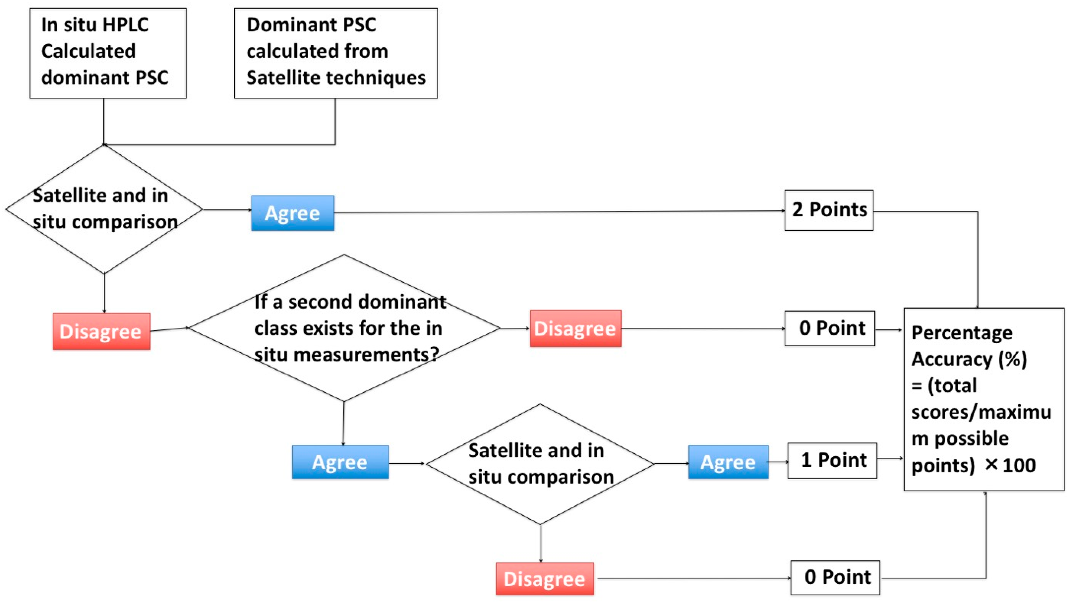
2.4. Accuracy Assessment

The accuracy of satellite derived Chla and aph were assessed by calculating the percentage error (PE), mean absolute percentage deviation (MAPD) and mean percentage deviation (MPD) between measured and derived values, using the following equations:
PE = 100 % · x d x m x m
MAPD = 100 % · 1 n i = 1 n | x d x m x m |
MPD = 100 % · 1 n i = 1 n x d x m x m
where xm is the measured value, xd is the derived value and n is the total number of samples.

3. Results

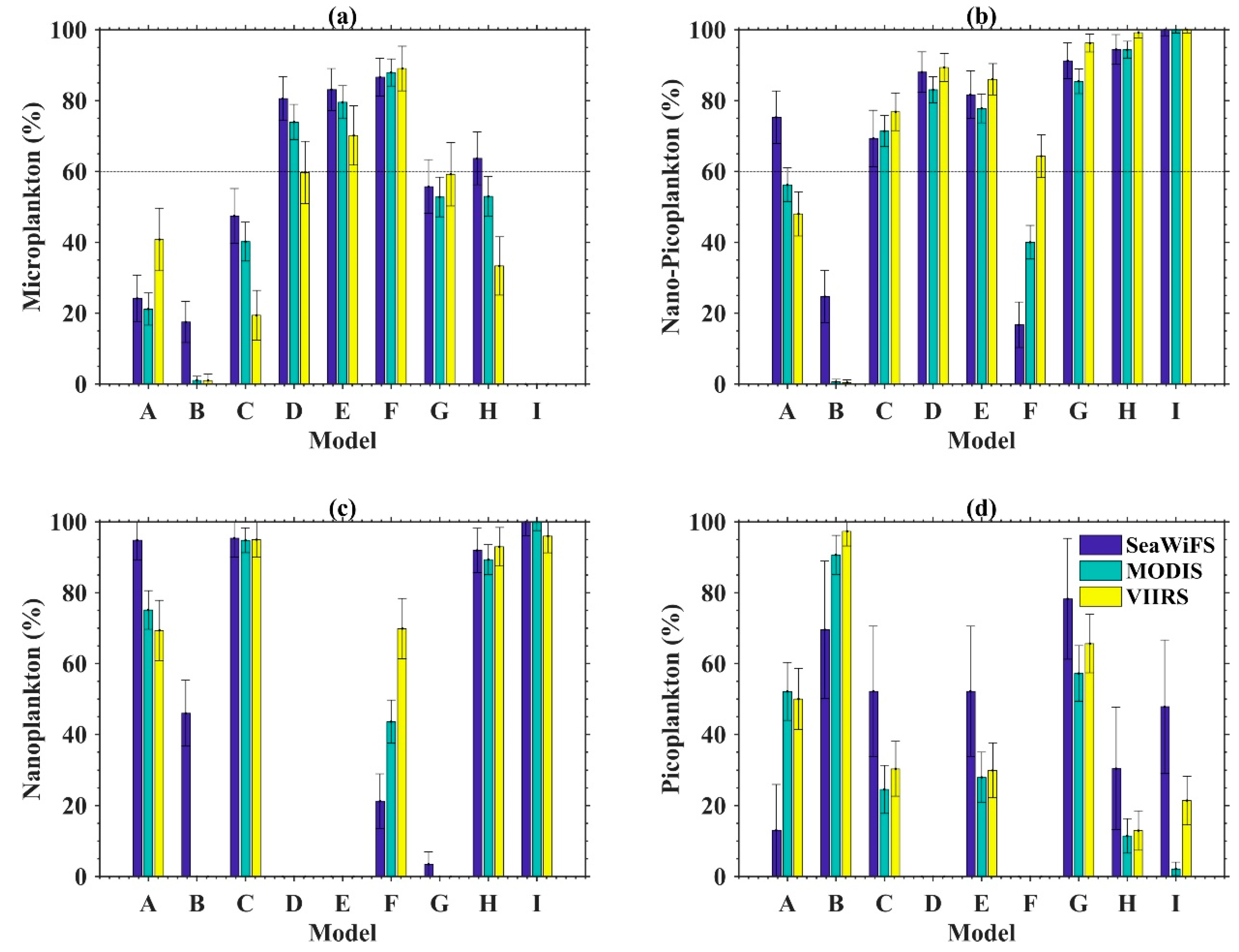
3.1. PSC Algorithm Comparison Results

3.1.1. SeaWiFS

The nine models were applied to SeaWIFS, MODIS, and VIIRS datasets, and a comparison of the percentage accuracy was carried out (Table 3 and Figure 5). Among the models applied to SeaWIFS data, D, E, and F showed relatively high accuracy (>80%) for the microphytoplankton size class, followed by G and H (55.7~63.7%). The performance of models A, B, C, and I was found to be relatively low (0~47.5%).
None of the models performed well for both nanophytoplankton and picophytoplankton (details below), and therefore a comparison of model performance for mixed nano–pico phytoplankton was made by treating the above models as two-population models (microphytoplankton and mixed nano–pico phytoplankton). Models D, E, G, H, and I were found to perform with higher accuracy (81.7~100%) than models A, B, C, and F (16.7~75.3%) although models A and C were not greatly different from model E.
For the nanophytoplankton size class, the performing accuracy of models A, C, H, and I (92.0~100%) were much higher than those of models B, E, F, and G (0~46.0%). For the picophytoplankton size class, the performing accuracy for all of the models was low, among which models B, C, E, G, and I performed with relatively higher accuracy (52.2~78.3%) than the rest of the models (13.0~47.8%).
The performance of models B, C, and D was evaluated using a global dataset in Brewin, et al. [30] (Table 3). The performance of the models was higher with the global dataset than with the dataset used in the present study, except for identification and estimation of the nanophytoplankton class. This could be explained by the fact that our in situ dataset is biased towards high Chla concentration (mesotrophic to eutrophic waters, Figure 3).

3.1.2. MODIS

For microphytoplankton-dominated populations, the accuracy of the nine algorithms applied to MODIS data was generally the same as found when using SeaWiFS: Models D, E, and F exhibited higher accuracy (74.0~87.9%) than models G and H (52.8~53.0%), followed by models A, B, C, and I (0~40.2%). Regarding the mixed nano–pico phytoplankton size classes, models C, D, E, G, H, and I performed with higher accuracy (71.4~100%) than models A, B, and F (0.6~56.2%).
For nanophytoplankton dominated populations, the accuracy of models A, C, H, and I were relatively high (75.1~100%) among the nine models, followed by model F (43.6%). The accuracy of models B, E, and G at retrieving dominance of nanophytoplankton was null. Regarding picophytoplankton dominated populations, model B exhibited the highest accuracy among all of the models (90.7%), followed by models G (57.2%) and A (52.1%), models C, E, H, and I exhibited relatively low accuracies (0~28%).

3.1.3. VIIRS

Among the models applied to VIIRS data in microphytoplankton dominated samples, models D, E, F, and G (59.2~89.1%) exhibited higher accuracy than models A, B, C, H, and I (0~40.8%). For mixed nano–pico phytoplankton populations, models C, D, E, G, H, and I (76.8~100%) performed with higher accuracy than models A, B, and F (0.42~64.3%). For nanophytoplankton dominated populations, the accuracy of models C, H, and I were highest (93~96%) among the nine models, followed by model A and F (69.3% and 69.8%, respectively). The accuracy of models B, E, and G were all found to be null. For picophytoplankton dominated samples, model B performed with the highest accuracy (97.3%), followed by models A and F (50.0~65.6%), and then models C, E, G, H, and I (0~30.4%).
Taking all of the satellite sensors and three phytoplankton size classes into consideration, none of the models performed with reasonable accuracies (e.g., >60%) at retrieving all three of the micro- nano-, and pico- phytoplankton size classes together. In other words, retrieving one size class accurately is achieved at the expenses of accurately retrieving another class(es). If we consider SeaWiFS and two populations (i.e., microphytoplankton and mixed nano–pico phytoplankton), models D, E, and H achieve greater than 60% accuracy for both size classes in the NWA. When the three sensors and two-population models were accounted for, model E was the only one that performed with a greater than 60% accuracy for both size classes.

4. Discussion

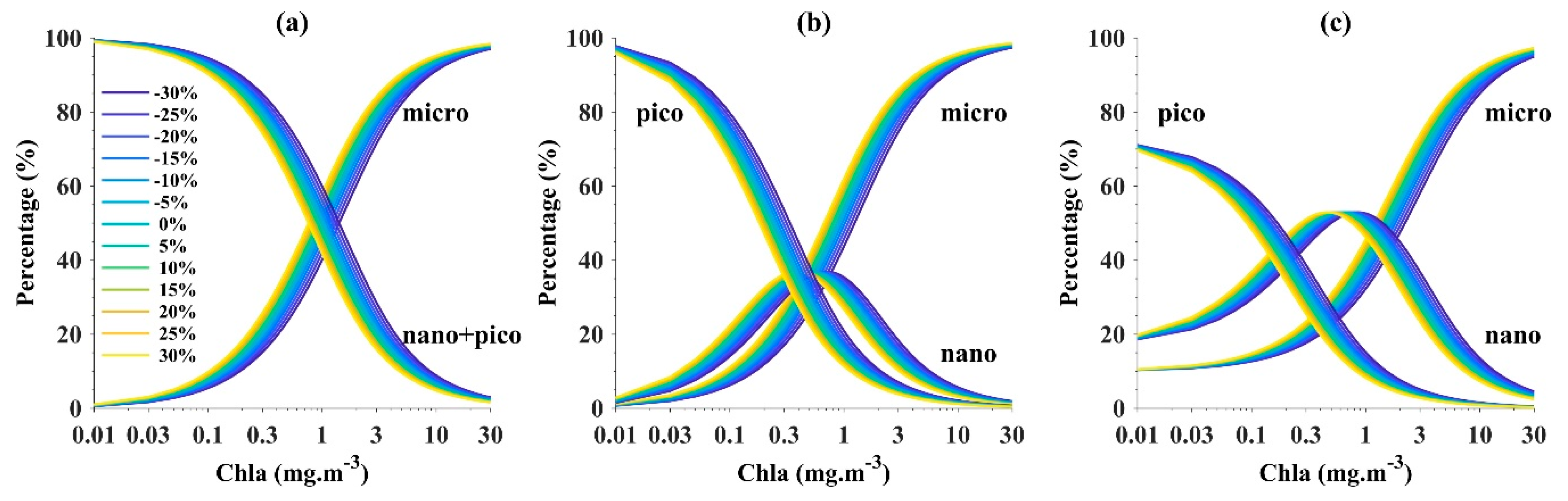
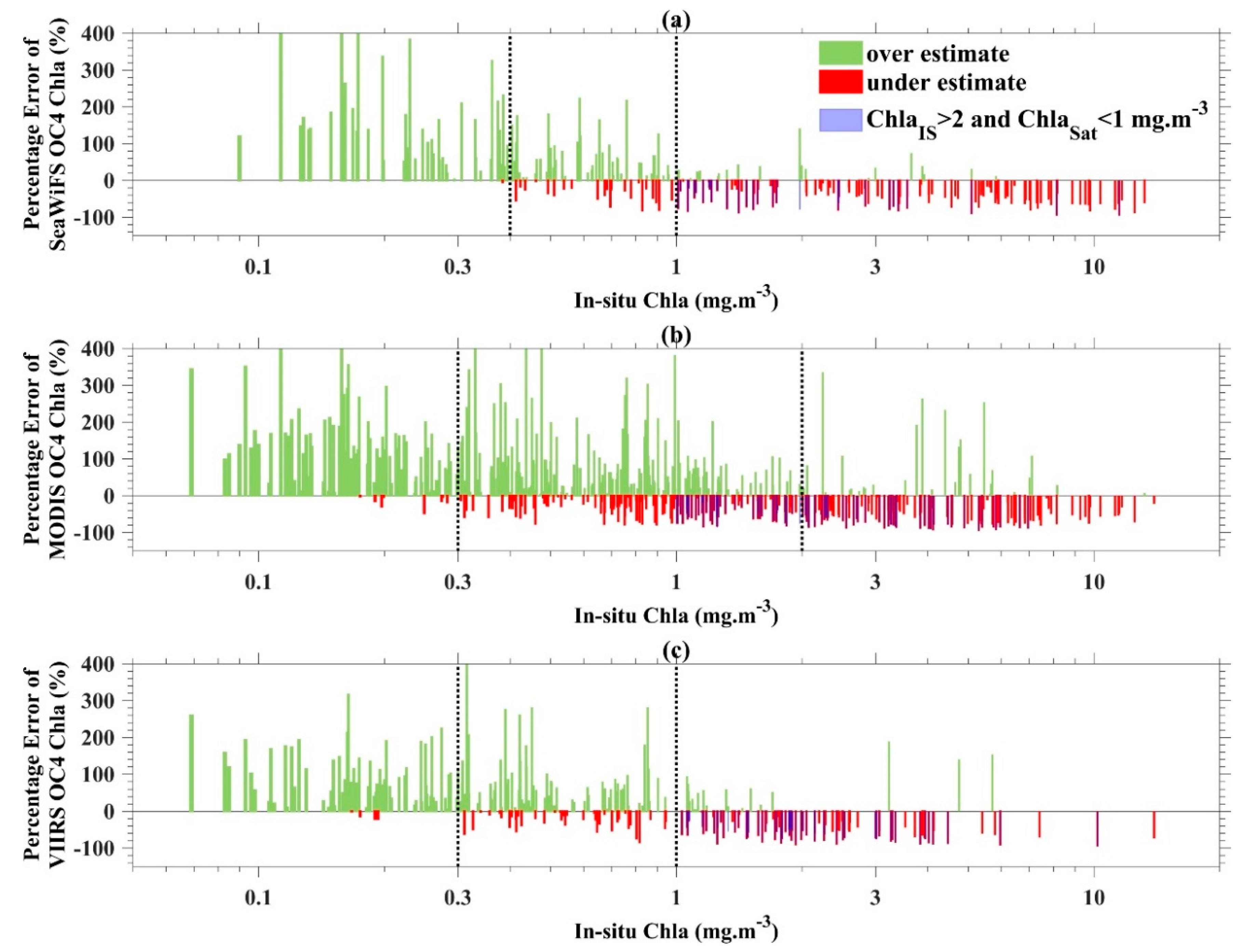
4.1. Uncertainties Associated with Satellite-Derived Inputs

4.1.1. OCx Chla Products

Models C, D, E, H, and I are all based on Chla, and in the case of model I, also SST, and therefore the accuracy of satellite Chla products is critical for phytoplankton size classification. The dominant PSC of Model C is based on thresholds of Chla. For models D, E, and H, the variation of each phytoplankton size class was defined as a non-linear function of Chla. However, for a given model and set of parameters, dominance of one group over others is always set by a given Chla (Figure 6), and thus dominance of a given phytoplankton class in these models is assessed similarly to a threshold algorithm such as model C.
For model D, samples with Chla less than 1 mg·m−3 were classified as mixed nano–pico phytoplankton dominated; whereas those with Chla greater than 1 mg·m−3 were classified as dominated by microphytoplankton (Figure 6a). For model E with the parameters used here, the maximum fraction of the nanophytoplankton size class that can be achieved is less than 45% (~40%, Figure 6b). This means that the criterion of dominant size class defined as greater than 45% is never realized and therefore model E was unable to retrieve nanophytoplankton as a dominant size class. In model E, samples with Chla values less than 0.3 mg·mg−3 were classified as picophytoplankton dominated, while those with Chla values greater than 1 mg·m−3 were classified as microphytoplankton dominated. Model H (Figure 6 c) classified the dominant PSC was classified as picophytoplankton when Chla was lower 0.15 mg·m−3, nanophytoplankton when Chla ranged between 0.15 and 1.5 mg·m−3, and microphytoplnakton when Chla > 1.5 mg·m−3.
In order to evaluate the impact of Chla on the estimation of PSC, a sensitivity analysis was also conducted (Figure 6). Here, we assumed that the Chla varies within a range of ±30%, which is the targeted accuracy for satellite-derived Chla in open oceans. When Chla had a positive bias, the microphytoplankton was overestimated in all three models (models D, E, and H), but the mixed nano–pico phytoplankton (model D) and picophytoplankton (models E and H) were underestimated. It is worth pointing out that when Chla had a positive bias, the nanophytoplankton was overestimated for the low Chla (<~0.5 mg·m−3) but underestimated for high Chla (~0.5 mg·m−3) (Figure 6b,c). The opposite was true when the Chla had a negative bias.
The error of satellite-derived Chla products is biased such that Chla is mainly overestimated when in situ Chla is low and underestimated when it is high (Figure 7). As expected, similar patterns of bias were observed for all three sensors. SeaWiFS OCx Chla was generally overestimated when in situ Chla concentration was less than 0.4 mg·m−3, while SeaWiFS OCx Chla was underestimated when in situ Chla was over 1 mg·m−3. For MODIS OCx Chla, the PE was generally positive when in situ Chla was less than 0.3 mg·m−3, and a systematic underestimation occurred when in situ Chla was greater than 2 mg·m−3. For the VIIRS OCx product, a systematic overestimation occurred when in situ Chla was less than 0.3 mg·m−3, and a systematic underestimation was observed when in situ Chla was greater than 1 mg·m−3.
Both the relationships between PSC and Chla and the uncertainties associated with satellite-derived Chla explain the poor performance of the abundance-based models to infer nano- and pico-phytoplankton on the NWA continental shelf (Figure 6 and Figure 7). On one hand, given the systematic overestimation of Chla by the OCx algorithm for Chla below 0.3 mg·m−3, in situ samples identified as picophytoplankton dominant can be misclassified as nanophytoplankton or even microphytoplankton dominated (Figure 6 and Figure 7). On the other hand, despite the underestimation of satellite-derived Chla using the OCx algorithm for in situ Chla above 2 mg·m−3, the outcome of the abundance-based models remained accurate for the microphytoplankton dominated size class, even considering the vast range of Chla (>1 mg·m−3, Figure 6) for the microphytoplankton dominated region. The in situ samples identified as microphytoplankton dominant but vulnerable to be misclassificated as nano- or pico- phytoplankton dominated (in situ Chla >2 mg·m−3 and satellite Chla <1 mg·m−3) were identified using blue bars in Figure 7.

4.1.2. Phytoplankton Absorption Coefficient Products

Models A, B, F, and G were based on absorption coefficient products. Two IOP models were selected to calculate aph from Rrs, EOF_NWA and QAA_v5. The PE of satellite-derived aph at 443, 490 and 555 nm compared to in situ data was further evaluated to help understand the impact of absorption retrieval on the performance of the algorithms. For all three satellite sensors (i.e., SeaWiFS, MODIS, and MERIS), the EOF-NWA model provided better statistical metrics for aph retrieval than the QAA model (Figure 8), specifically, a narrower distribution of PE and lower values of MAPD ranging from ~35% to ~47%. The aph derived from QAA_v5 shows a relatively wide distribution of PE, with most of MAPD higher than 76%. In particular, the EOF_NWA model showed positive MPD for all of three bands of the three satellite sensors (9.4~25.15%), demonstrating a slight overestimation with this model (Figure 8). For the QAA_v5 model, systematic negative MPD values were found for all three wavebands for all three satellite sensors (−29.6~−78.7%), with the exception of 490 and 555 nm wavebands of SeaWiFS. This demonstrated an overall underestimation on aph with the QAA_v5 model (Figure 8).
The original version of QAA was used in our analyses and no regional parameterization was performed, which may explain the relatively poor performance of this method when tested on a regional dataset. Similar to our findings, Shanmugam, et al. [48] showed that phytoplankton absorption coefficients retrieved by QAA were generally underestimated for the selected wavebands (412, 443, 490, 510, and 555 nm) in coastal regions. The underestimation revealed by Shanmugam, et al. [48] (as well as in our study) was attributed to the spectral slope of colored dissolved organic matter absorption (aCDOM) and detritus (ad), which resulted in an overestimation of aCDOM and ad, and corresponding underestimation of aph at these wavelengths. In agreement with previous works [25,26], our results suggest that a regional parameterization of IOP models by a fully suited dataset is required in our region of study.

4.2. Model Selection for Monitoring PSC in the NWA

Our results showed that dominance of microphytoplankton and mixed nano–pico phytoplankton populations (i.e., two-population model) in the NWA were more accurately detected than three-population classifications (Figure 5). This might be due to (i) the abundance-based models’ reliance on low Chla values to detect nano- and picophytoplankton and the OCx algorithms’ systematic overestimation of Chla at low concentration (i.e., Chla < ~0.3/0.4 mg·m−3) (Figures 7), and (ii) productive waters in the study areas, in which oligotrophic conditions are under-represented in the in situ dataset (Figure 3).
Among the three different approaches, abundance-based and spectral-based models performed better than the ecological-based model (model I), which tended to over classify pixels in the nanophytoplankton size class in the region of interest. The ecological-based model, based on phytoplankton biomass, was developed to retrieve PSCs over large spatial scales, limiting the application of these large-scale empirical ecological relationships, which were rather scattered with low determination coefficients, as is shown in Barnes, et al. [28], to the relatively small shelf region.
The performance of the absorption-based models (e.g., A, B, F, and G) depends on the IOP model selected. Models A and F, which used the EOF_NWA approach to derive phytoplankton absorption, performed better at detecting microphytoplankton and nanophytoplankton dominated pixels than the picophytoplankton dominated pixels. The derived phytoplankton absorption by EOF_NWA is, on average, overestimated, which results in an underestimation of picophytoplankton. Models B and G that had inputs calculated according to QAA_v5 [42], worked better at detecting picophytoplankton dominated pixels than those dominated by the other two size classes. This is a result of the systematic underestimation of aph by QAA_v5, compared to estimates by EOF_NWA (Figure 8).
Compared to open ocean, the 3-class PSC models showed relatively poor performance in coastal waters (Scotian Shelf, Northwest Atlantic), in particular for the picophytoplankton class ([30] and Table 3 in this study). This phenomenon is mainly a result of: (a) The larger uncertainty of the Chla product in productive waters compared to the open ocean, and the possible contamination of yellow substance absorption to the total water leaving signal, known to artificially increase Chla in band-ratio algorithms; and (b) under-representation of samples dominated by picophytoplankton in coastal regions (Figure 3) since they generally dominate in oligotrophic waters. Therefore, the application of the models to productive waters must be handled cautiously and would benefit from regional adjustment.
Regarding the use of HPLC-based PSC as a reference, several limitations exist that have to be accounted for when interpreting the results. Some marker pigments are shared among several phytoplankton taxa, making it difficult to identify different groups unambiguously. For example, Chlb is the marker pigment for green flagellates and prochlorophytes [49,50,51,52]. However, it is also present in Euglenophyta, which is classified as nano- or micro-phytoplankton [12]. In addition, the HPLC-based phytoplankton size class determination is sensitive to assumptions about the Chla to diagnostic pigment ratios [1,13,14]. Therefore, uncertainties of the in situ data are not negligible. None of the current in situ methods to identify phytoplankton taxa or functions (such as microscopy, flow cytometry, and filtration etc.) are considered ideal for detection and quantification of PSC [1]. A compromise has to be achieved between the accuracy at retrieving information of phytoplankton against the range covered by the method used. For instance, while microscopic counts and flow cytometry have high accuracy of measurements, these methods are constrained by the phytoplankton cell size they can resolve (~5 to 300 μ m and 0.2 to ~20 μ m for light microscopy and flow cytometry respectively). Conversely, HPLC-derived pigment composition and concentration resolve the entire size range of the bulk phytoplankton population but have less capacity to identifying phytoplankton groups accurately. Here we have relied on HPLC pigment information, one of the most widely used measurements in the field of marine optics/biogeochemistry. It is also noteworthy that PSC models that were developed using HPLC-pigment database are the ones that provide the best results, which advocate for an independent measurement to truly assess the performance of these algorithms. In addition, it is expected that models developed using regional datasets will perform better than those developed using global datasets. However, some global models, such as Brewin et al. (2010) showed that they could still be applied on the NWA continental shelf with meaningful results.

4.3. PSC in Northwest Atlantic

Our results revealed that none of the PSC models tested were sufficiently accurate in retrieving the three PSCs simultaneously (micro-, nano-, and pico- phytoplankton). It appears that for any given algorithm, successfully retrieving information on a particular size class is achieved at the expense of other classes, meaning that an algorithm that performs well to retrieving the fraction of microphytoplankton will do so at the expense of retrieving nano- or pico-phytoplankton fractions accurately. When we applied the stringent criteria of at least 60% accuracy in retrieving two size class fractions (microphytoplankton and mixed nano–pico phytoplankton) for all three sensors, only model E performed successfully. The above average performance of model E is not a surprise since: (a) simpler models tends to be more robust; and (b) it was developed using a dataset from this NWA region (spanning 1996–2003). Given the inverse relationship between the microphytoplankton and mixed nano–pico phytoplankton classes (see Equation (2)), only the time series analysis of CCI-derived microphytoplankton fraction percentage is reported here.

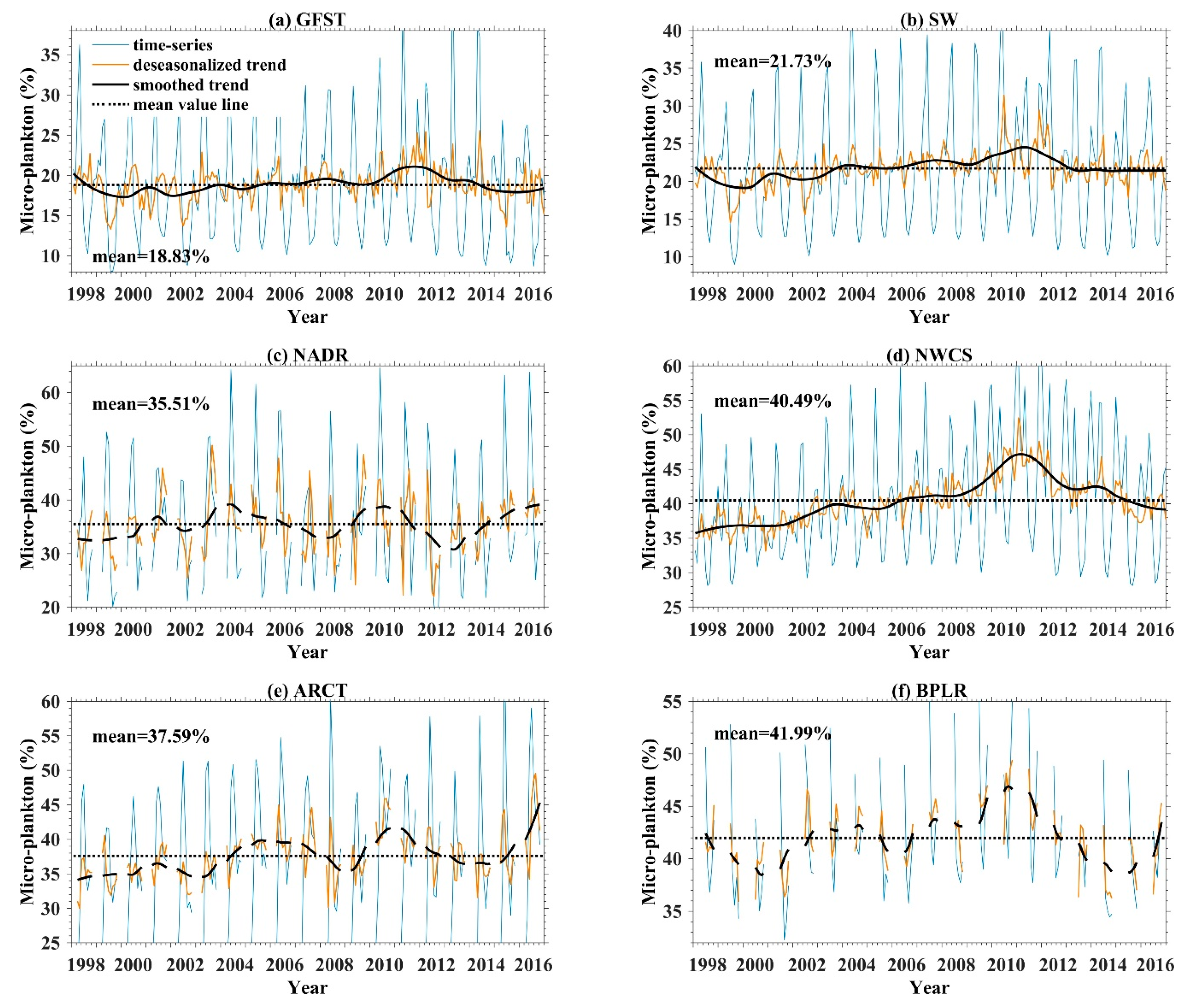
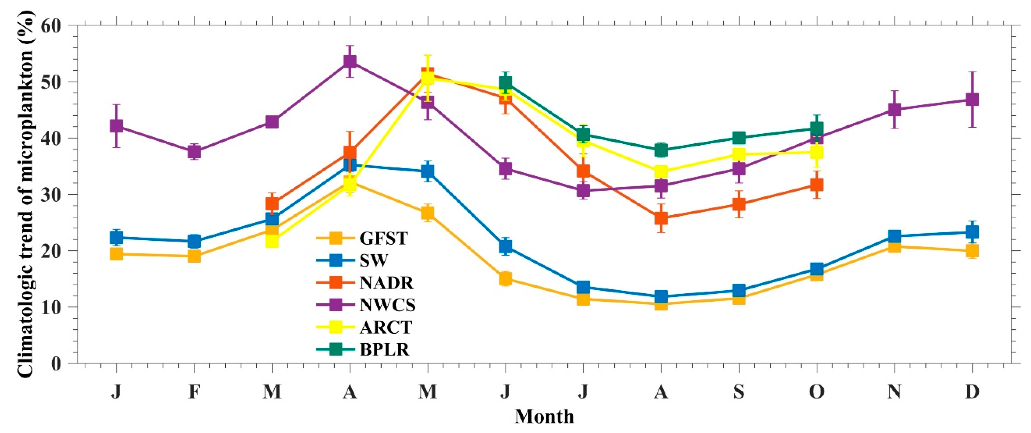
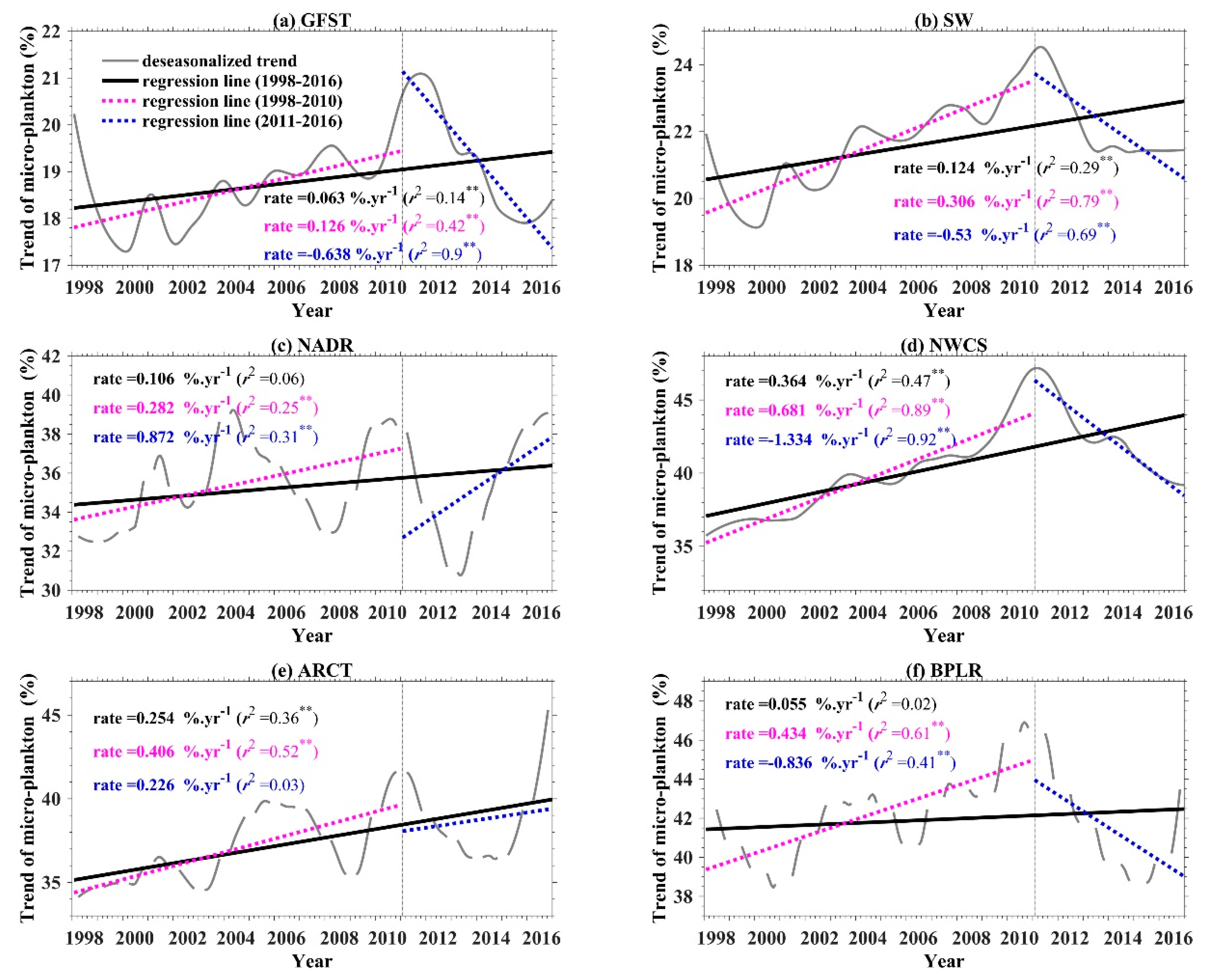
4.3.1. Temporal Variation of Microphytoplankton in NWA

Time-series of microphytoplankton fractions in the six ecological provinces were decomposed into three components (seasonal cycle, trend, and residual) to detect possible long-term changes in phytoplankton community structure (Figure 9, Figure 10 and Figure 11). For the three southern provinces, the highest average microphytoplankton fraction from 1998 to 2016 was showed in most productive region NWCS (40.49%), then followed by SW (21.73%) and GFST (18.83%) (Figure 9a,b,d). The seasonal cycles in microphytoplankton fraction in NWCS, SW, and GFST had pronounced peaks in April (NWCS, GFST) or April–May (SW), corresponding to the spring bloom timing. This is followed by an abrupt decrease in the fraction of microphytoplankton, which last the entire summer and early fall, and a less intense secondary bloom occurring around November–December (late fall, early winter) (Figure 9 and Figure 10). In the GFST and SW, the microphytoplankton cycle was less pronounced than in the NWCS, with the microphytoplankton fraction reaching at most 30% in the spring compared to a value of 60% in the NWCS (Figure 9 and Figure 10). The seasonal cycles in NADR, ARCT, and BPLR were truncated due to the presence of ice cover in winter months that prevent recording of satellite ocean-colour measurements. The peak of the microphytoplankton fraction occurred between May and June in the three provinces. In the NADR and ARCT provinces, the mean values between March and October from 1998 to 2016 were 35.51% and 37.59% respectively (Figure 9c,e). In BPLR, the mean value between June and October in the 19 years was 41.99% (Figure 9f).
For four of the six provinces (GFST, SW, NWCS, and BPLR) the trend in microplankton fraction showed an increase from the late 1990s to approximately 2010 followed by a sharp decline (Figure 11a,b,d,f). The two remaining provinces (ARCT and NADR) exhibited a less pronounced decrease after 2010, which lasted 2 to 4 years, before oscillating positively again (Figure 11c,e). Therefore, in addition to the temporal analysis over the entire period of observation (19 years, 1998–2016), we studied the trends of the time series for each province for two distinct periods corresponding to 1998–2010 and 2011–2016 (Figure 11). In general, the trend for the microphytoplankton fraction in GFST, SW, and NWCS were similar, with a significant increase until 2010s followed by a decrease, although there was an overall increasing trend over the full 19 year time-series (Figure 11a,b,d). Over the 19 years of observation, the slope of the microphytoplankton fraction versus time (in year) was positive and significant (p < 0.001) for four provinces, including NWCS (0.36%·yr−1), ARCT (0.25%·yr−1), SW (0.12%·yr−1), and GFST (0.06%·yr−1), and positive but not significant for BPLR (0.06%·yr−1) and NADR (0.11%·yr−1). From 1998 to 2010 the trends in all six provinces showed a positive slope with higher values found for the coastal provinces: NWCS (0.68%·yr−1), BPLR (0.43%·yr−1), and ARCT (0.41%·yr−1) and smaller positive slopes for the pelagic provinces in descending order from the least to the most oligotrophic. After 2010, the relative abundance trends of microphytoplankton were negative in NWCS (−1.33%·yr−1), BPLR (−0.84%·yr−1), GFST (−0.64%·yr−1), and SW (−0.53%·yr−1). However, a significant positive slope was found in the NADR (0.87%·yr−1) and a positive slope in ARCT (0.23%·yr−1, p > 0.001) for the second truncation of the time-series.

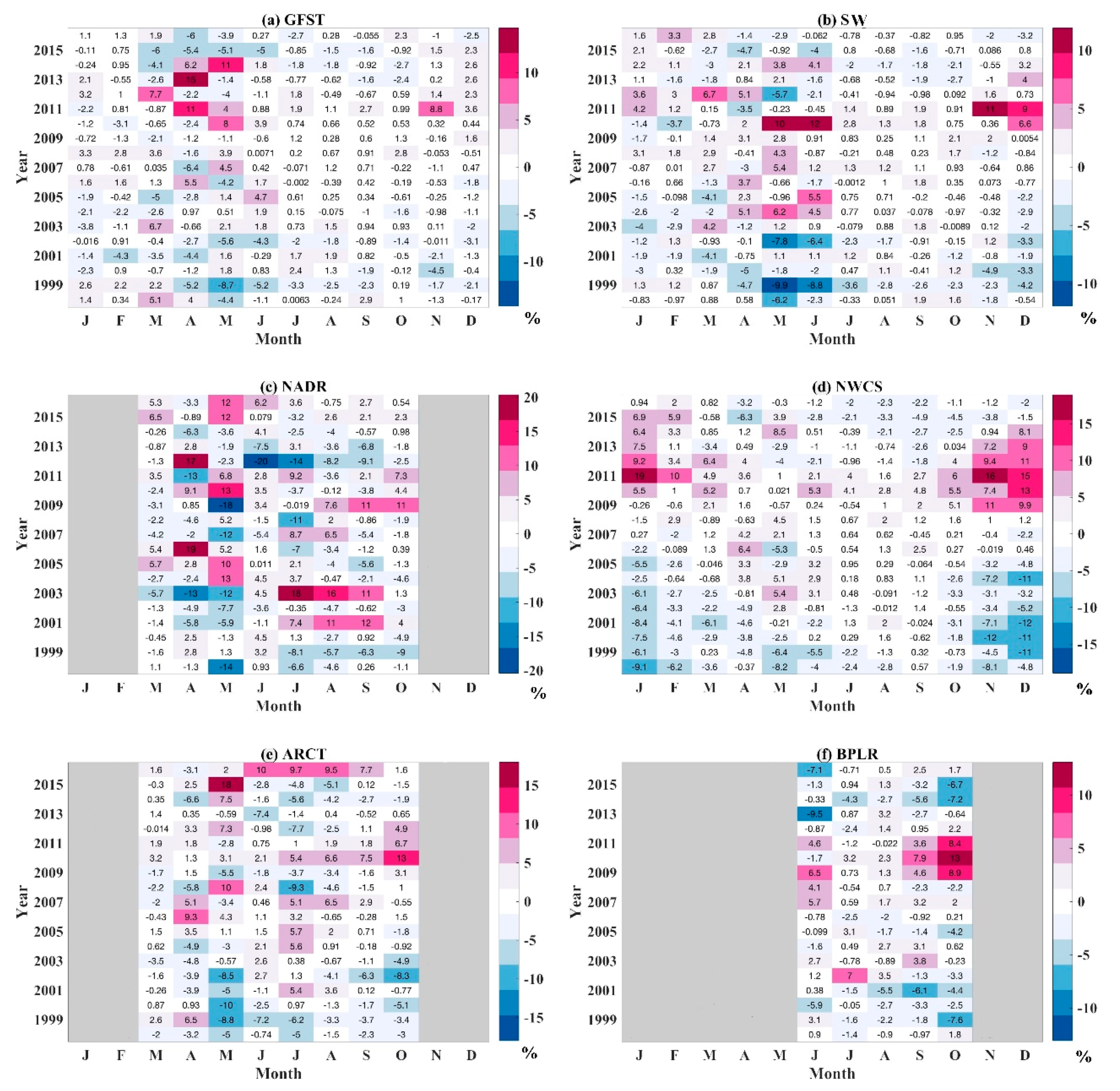
4.3.2. Anomaly Analysis of Microphytoplankton in NWA

Overall annual trends of microphytoplankton fraction in the six provinces conceal large variation in the seasonal signal. Percentage anomalies of microphytoplankton in each ecological province are shown in Figure 12. The anomaly was calculated by subtracting the overall mean of each month (1998 to 2016) from each cell. In GFST, the anomalies from March to May showed the largest variations, positive values were found from March to May between 2010 and 2014 (Figure 12a). Generally, the anomaly in SW was negative before 2003, predominantly positive anomalies were found in 2010 and 2011(Figure 12b). In NADR, the anomalies showed a vast variation (Figure 12c). The NADR province represents a boundary area influenced by BPLR, NWCS, and SW waters [34], resulting in a highly dynamic climatological character. In NWCS, the anomalies were negative before 2006, while between 2008 and 2013 positive anomalies were observed in winter months (Figure 12d). It is noteworthy that the anomalies were all positive in 2011, which is consistent with the pronounced peak in 2011 for the time-series analysis results in NWCS (Figure 11d and Figure 12d). In ARCT, the anomalies showed positive values in 2010 and 2016, while negative anomalies were generally found before 2003, which is consistent with the trend shown in Figure 11e. In BPLR, the anomaly of microphytoplankton in September and October was positive from 2009 to 2011 (Figure 12f), which corresponds to the peak of the time-series trend within these years (Figure 11f).

4.3.3. Discussion on the Microphytoplankton Variation in NWA

Model E, was selected following the performance assessment study of nine PSC models. However, this study focused only on the ability of the models to derive the dominant PSCs, and not the accuracy of the retrieval of the PSCs. Therefore, we further compared the in situ and CCI-derived microphytoplankton (both concentration and fraction), to test the performance of model E (Figure 13). The in situ and CCI-derived microphytoplankton are consistent with each other, with a highly significant linear relationship for both concentration and fraction (r2 = 0.73 and 0.72, respectively, p-value < 0.01). As observed with Chla concentration derived from ocean colour satellite, a systematic overestimation for microphytoplankton concentration and fraction was observed when in situ Chla was lower than ~0.5 mg·m−3, while CCI-derived values were generally underestimated when in situ Chla was higher than ~ 0.5 mg·m−3. Given that model E is an abundance-based model, the overestimation in the lower-end and the underestimation in the higher-end of the Chla concentration spectrum result from uncertainties in the OCx Chla algorithm (Figure 6, Figure 7 and Figure 13). Indeed, this uncertainty on Chla directly propagate to microphytoplankton estimates. However, the effect of this systematic bias will not change the sign of long-term trends in each ecological province, but perhaps decrease its magnitude.
Our findings on microphytoplankton variation in NWA are consistent with the results of a remote-sensing-based study of phytoplankton phenology from 1998 to 2012 that identified a shift toward earlier spring bloom timing in the NWCS in recent years as well as increasing magnitude of fall/winter blooms in the entire NWA [53]. A comprehensive analysis of factors influencing phytoplankton phenology in the North Atlantic (including SST, photosynthetic active radiation, wind stress, and eddy kinetic) revealed that SST was the main driver of the deviance in inter-annual winter bloom magnitude in the NWA [53]. Between 2012 and 2014, SST anomalies (based on a 1985–2010 climatology) from July to November remained positive for the majority of the NWA region [54,55,56]. In contrast, in 2015 and 2016, SST anomalies from July to November in the ARCT and the Northwest of NWCS were negative [57,58]. This is consistent with the pronounced “fall-winter peak” in the fraction of microphytoplankton recorded in the early 2010s for the NWCS and ARCT provinces, and the relatively low microphytoplankton anomalies recorded in the winter months of 2015 and 2016 there (Figure 12c–e).
A previous study based on Continuous Plankton Recorder (CPR) data collected from 1958–2006 characterized variability in surface-water diatom and dinoflagellate abundance in an area corresponding to the NWCS [59]. Diatom abundance was higher in the 1990s and early 2000s than in the 1960s and 1970s in regions corresponding to the NWCS, due mainly to differences in abundance in the winter months [59]. The abundance of dinoflagellates was also significantly higher in the 1990s and early 2000s than in previous decades, but the differences were driven by shifts in abundance mainly in the first half of the year on the Scotian Shelf and throughout the year on the Newfoundland Shelf [59]. In our study, an increase of microphytoplankton fraction in the NWCS was observed in winter months in 2010s relative to the 2000s (Figure 12). In this context, although the methodologies and spatial coverage employed by these two studies were different, a general conclusion can be drawn that the fraction of microphytoplankton had been increasing in the last three or four decades, with a reversal in the trend around 2010. The increase in CPR-based diatom abundance in the 1990s and 2000s was attributed to higher stratification in the winter, which would enhance phytoplankton production by stabilizing the water column at a time when strong mixing would normally inhibit production [59]. In our study, persistent higher than average fall–winter microphytoplankton fractions were observed from 2009 to 2014, even as the trend in microphytoplankton fraction became negative due to below-average fractions observed in the summer, when stronger stratification would reduce the supply of nutrients to the euphotic zone and inhibit production of large phytoplankton. A decline in deep-water silicate concentrations that started in 2013 may have further inhibited production of diatoms [35].

5. Conclusions

Nine Phytoplankton Size Class (PSC) models were evaluated against in situ observations in the Northwest Atlantic (NWA). The PSC models’ performance was lower in productive waters (Scotian Shelf, Northwest Atlantic; within 4 degrees of the coastline) compared to the results obtained from the global open ocean. Model performance was especially poor for picophytoplankton-dominated communities (Table 3). This could be related to large errors in satellite-derived model inputs (e.g., Chla concentration and absorption coefficient of phytoplankton), and a general under-representation of pico-dominated samples in productive waters. Considering the accuracy of retrieving micro- and mixed nano–pico phytoplankton, Devred et al. 2011 [25] (model E) showed the best performance among the nine models for the three satellite products (i.e., SeaWiFS, MODIS, and VIIRS), which is not surprising given that this model was developed including a regional dataset.
The best performance model was then applied to the NWA daily OC-CCI images from 1998 to 2016, to demonstrate the spatial and temporal variations of microphytoplankton fraction. For the three southern ecological provinces, there was a significant increase in the microphytoplankton fraction until 2010s followed by a decrease, although there was an overall increasing trend over the full 19 year time-series. Strong anomalies in winter months between 2008 and 2013 were found in Northwest Continental Shelf, which could be driven by the changes in environmental factors (e.g., SST, stratification, and nutrient supply).
In a changing climate, long-term dynamics on the PSC variations would aid in the monitoring and investigating of water system changes. In addition, in our studied area, the selected model can be also applied at a smaller scale in representative areas and compared with changes in environmental drivers at more relevant scales, to further reveal the influence of environmental factors on the changes of PSC. Besides, our study indicates that the application of PSC models to productive waters has its limitations. As an active area of research, new ocean-color-based PSC models are under development. Ongoing efforts strive to include more data, more diverse conditions, and to improve model formulation and parameterization. Improved (both methodologically and quantitatively) in situ observations and satellite products in productive waters together will help to advance PSC research in the future.

Author Contributions

E.D. and C.J. conceived and designed the experiments; X.L., E.D., and C.J. performed the experiments; X.L. and E.D. analyzed the data; E.D. contributed reagents/materials/analysis tools; X.L. wrote the paper; E.D. and C.J. edited the paper.

Funding

This work was funded by the Strategic Program for the Ecosystem-based Research and Advice (SPERA) program.

Acknowledgments

We would like to thank Reba McIver, Stephanie Clay, and Carla Caverhill for their help in data processing.

Conflicts of Interest

The authors declare no conflict of interest.

References

  1. International Ocean-Colour Coordinating Group (IOCCG). Phytoplankton Functional Types from Space; International Ocean-Colour Coordinating Group: Dartmouth, NS, Canada, 2014. [Google Scholar]
  2. Sieburth, J.M.; Smetacek, V.; Lenz, J. Pelagic ecosystem structure: Heterotrophic compartments of the plankton and their relationship to plankton size fractions. Limnol. Oceanogr. 1978, 23, 1256–1263. [Google Scholar] [CrossRef]
  3. Marañón, E. Cell size as a key determinant of phytoplankton metabolism and community structure. Annu. Rev. Mar. Sci. 2015, 7, 241–264. [Google Scholar] [CrossRef] [PubMed]
  4. Finkel, Z.V.; Beardall, J.; Flynn, K.J.; Quigg, A.; Rees, T.A.V.; Raven, J.A. Phytoplankton in a changing world: Cell size and elemental stoichiometry. J. Plankton Res. 2009, 32, 119–137. [Google Scholar] [CrossRef]
  5. Irwin, A.J. Scaling-up from nutrient physiology to the size-structure of phytoplankton communities. J. Plankton Res. 2006, 28, 459–471. [Google Scholar] [CrossRef] [Green Version]
  6. Nair, A.; Sathyendranath, S.; Platt, T.; Morales, J.; Stuart, V.; Forget, M.-H.; Devred, E.; Bouman, H. Remote sensing of phytoplankton functional types. Remote Sens. Environ. 2008, 112, 3366–3375. [Google Scholar] [CrossRef]
  7. Key, T.; McCarthy, A.; Campbell, D.A.; Six, C.; Roy, S.; Finkel, Z.V. Cell size trade-offs govern light exploitation strategies in marine phytoplankton. Environ. Microbiol. 2010, 12, 95–104. [Google Scholar] [CrossRef] [PubMed]
  8. Kirk, J.T.O. Light and Photosynthesis in Aquatic Ecosystems, 3rd ed.; Cambridge University Press: Cambridge, UK, 2011; ISBN 978-0-521-15175-7. [Google Scholar]
  9. Morel, A.; Bricaud, A. Theoretical results concerning light absorption in a discrete medium, and application to specific absorption of phytoplankton. Deep Sea Res. Part A Oceanogr. Res. Pap. 1981, 28, 1375–1393. [Google Scholar] [CrossRef]
  10. Chisholm, S.W. Phytoplankton size. In Primary Productivity and Biogeochemical Cycles in the Sea; Springer: New York, NY, USA, 1992. [Google Scholar]
  11. Roy, S.; Llewellyn, C.A.; Egeland, E.S.; Johnsen, G. Phytoplankton Pigments: Characterization, Chemotaxonomy and Applications in Oceanography; Cambridge University Press: Cambridge, UK, 2011. [Google Scholar]
  12. Jeffrey, S.; Mantoura, R.; Wright, S. Phytoplankton Pigments in Oceanography: Guidelines to Modern Methods; Unesco Publishing: Paris, France, 1997; ISBN 92-3-103275-5. [Google Scholar]
  13. Vidussi, F.; Claustre, H.; Manca, B.B.; Luchetta, A.; Marty, J.C. Phytoplankton pigment distribution in relation to upper thermocline circulation in the eastern Mediterranean Sea during winter. J. Geophys. Res. Oceans 2001, 106, 19939–19956. [Google Scholar] [CrossRef] [Green Version]
  14. Uitz, J.; Claustre, H.; Morel, A.; Hooker, S.B. Vertical distribution of phytoplankton communities in Open Ocean: An assessment based on surface chlorophyll. J. Geophys. Res. 2006, 111. [Google Scholar] [CrossRef]
  15. Hood, R.R.; Laws, E.A.; Armstrong, R.A.; Bates, N.R.; Brown, C.W.; Carlson, C.A.; Chai, F.; Doney, S.C.; Falkowski, P.G.; Feely, R.A. Pelagic functional group modeling: Progress, challenges and prospects. Deep Sea. Res. Part II Top. Stud. Oceanogr. 2006, 53, 459–512. [Google Scholar] [CrossRef] [Green Version]
  16. Quere, C.L.; Harrison, S.P.; Colin Prentice, I.; Buitenhuis, E.T.; Aumont, O.; Bopp, L.; Claustre, H.; Cotrim Da Cunha, L.; Geider, R.; Giraud, X. Ecosystem dynamics based on plankton functional types for global ocean biogeochemistry models. Glob. Chang. Biol. 2005, 11, 2016–2040. [Google Scholar] [CrossRef]
  17. Moloney, C.L.; Field, J.G. The size-based dynamics of plankton food webs. I. A simulation model of carbon and nitrogen flows. J. Geophys. Res. 1991, 13, 1003–1038. [Google Scholar] [CrossRef]
  18. Marinov, I.; Doney, S.C.; Lima, I.D. Response of ocean phytoplankton community structure to climate change over the 21st century: Partitioning the effects of nutrients, temperature and light. Biogeosciences 2010, 7, 3941–3959. [Google Scholar] [CrossRef]
  19. Sathyendranath, S.; Cota, G.; Stuart, V.; Maass, H.; Platt, T. Remote sensing of phytoplankton pigments: A comparison of empirical and theoretical approaches. Int. J. Remote Sens. 2001, 22, 249–273. [Google Scholar] [CrossRef]
  20. Kostadinov, T.S.; Siegel, D.A.; Maritorena, S. Retrieval of the particle size distribution from satellite ocean color observations. J. Geophys. Res. 2009, 114. [Google Scholar] [CrossRef] [Green Version]
  21. Loisel, H.; Nicolas, J.M.; Sciandra, A.; Stramski, D.; Poteau, A. Spectral dependency of optical backscattering by marine particles from satellite remote sensing of the global ocean. J. Geophys. Res. Oceans 2006, 111. [Google Scholar] [CrossRef] [Green Version]
  22. Sathyendranath, S.; Lazzara, L.; Prieur, L. Variations in the spectral values of specific absorption of phytoplankton. Limnol. Oceanogr. 1987, 32, 403–415. [Google Scholar] [CrossRef] [Green Version]
  23. Reynolds, R.A.; Stramski, D.; Mitchell, B.G. A chlorophyll-dependent semianalytical reflectance model derived from field measurements of absorption and backscattering coefficients within the southern ocean. J. Geophys. Res. Oceans 2001, 106, 7125–7138. [Google Scholar] [CrossRef]
  24. Alvain, S.; Moulin, C.; Dandonneau, Y.; Bréon, F.M. Remote sensing of phytoplankton groups in case 1 waters from global seawifs imagery. Deep Sea Res. Part I Oceanogr. Res. Pap. 2005, 52, 1989–2004. [Google Scholar] [CrossRef] [Green Version]
  25. Devred, E.; Sathyendranath, S.; Stuart, V.; Platt, T. A three component classification of phytoplankton absorption spectra: Application to ocean-color data. Remote Sens. Environ. 2011, 115, 2255–2266. [Google Scholar] [CrossRef]
  26. Devred, E.; Sathyendranath, S.; Stuart, V.; Maass, H.; Ulloa, O.; Platt, T. A two-component model of phytoplankton absorption in the open ocean: Theory and applications. J. Geophys. Res. 2006, 111. [Google Scholar] [CrossRef] [Green Version]
  27. Bricaud, A. Natural variability of phytoplanktonic absorption in oceanic waters: Influence of the size structure of algal populations. J. Geophys. Res. 2004, 109. [Google Scholar] [CrossRef] [Green Version]
  28. Barnes, C.; Irigoien, X.; De Oliveira, J.A.; Maxwell, D.; Jennings, S. Predicting marine phytoplankton community size structure from empirical relationships with remotely sensed variables. J. Plankton Res. 2011, 33, 13–24. [Google Scholar] [CrossRef]
  29. Palacz, A.P.; John, M.A.S.; Brewin, R.J.W.; Hirata, T.; Gregg, W.W. Distribution of phytoplankton functional types in high-nitrate low-chlorophyll waters in a new diagnostic ecological indicator model. Biogeosci. Discuss. 2013, 10, 8103–8157. [Google Scholar] [CrossRef] [Green Version]
  30. Brewin, R.J.W.; Hardman-Mountford, N.J.; Lavender, S.J.; Raitsos, D.E.; Hirata, T.; Uitz, J.; Devred, E.; Bricaud, A.; Ciotti, A.; Gentili, B. An intercomparison of bio-optical techniques for detecting dominant phytoplankton size class from satellite remote sensing. Remote Sens. Environ. 2011, 115, 325–339. [Google Scholar] [CrossRef]
  31. Di Cicco, A.; Sammartino, M.; Marullo, S.; Santoleri, R. Regional empirical algorithms for an improved identification of phytoplankton functional types and size classes in the mediterranean sea using satellite data. Front. Mar. Sci. 2017, 4, 126. [Google Scholar] [CrossRef]
  32. Kostadinov, T.S.; Cabré, A.; Vedantham, H.; Marinov, I.; Bracher, A.; Brewin, R.J.; Bricaud, A.; Hirata, T.; Hirawake, T.; Hardman-Mountford, N.J. Inter-comparison of phytoplankton functional type phenology metrics derived from ocean color algorithms and earth system models. Remote Sens. Environ. 2017, 190, 162–177. [Google Scholar] [CrossRef]
  33. Longhurst, A. The Atlantic Ocean; Elsevier Science Publishers: New York, NY, USA, 2006; pp. 131–268. ISBN 978-0-12-455521-1. [Google Scholar]
  34. Devred, E.; Sathyendranath, S.; Platt, T. Delineation of ecological provinces using ocean colour radiometry. Mar. Ecol. Prog. Ser. 2007, 346, 1–13. [Google Scholar] [CrossRef] [Green Version]
  35. Department of Fisheries and Oceans (DFO). Optical, Chemical, and Biological Oceanographic Conditions on the Scotian Shelf and in the Eastern Gulf of Maine in 2015; Fishery and Oceans Canada: Ottawa, Canada, 2017. [Google Scholar]
  36. Yentsch, C.S. Measurement of visible light absorption by particulate matter in the ocean. Limnol. Oceanogr. 1962, 7, 207–217. [Google Scholar] [CrossRef] [Green Version]
  37. Mitchell, B.; Kiefer, D. Determination of absorption and fluorescence excitation spectra for phytoplankton. In Marine Phytoplankton and Productivity; Springer: Berlin/Heidelberg, Germany, 1984; pp. 157–169. [Google Scholar]
  38. Hoepffner, N.; Sathyendranath, S. Effect of pigment composition on absorption properties of phytoplankton. Mar. Ecol. Prog. Ser. 1991, 73, 11–23. [Google Scholar] [CrossRef]
  39. Kyewalyanga, M.N.; Platt, T.; Sathyendranath, S. Estimation of the photosynthetic action spectrum: Implication for primary production models. Mar. Ecol. Prog. Ser. 1997, 146, 207–223. [Google Scholar] [CrossRef]
  40. Stuart, V.; Head, E.J. The Second Seawifs Hplc Analysis Round-Robin Experiment (Seaharre-2) (p. 112); NASA/TM: Greenbelt, MD, USA, 2005; p. 124. [Google Scholar]
  41. Craig, S.E.; Jones, C.T.; Li, W.K.W.; Lazin, G.; Horne, E.; Caverhill, C.; Cullen, J.J. Deriving optical metrics of coastal phytoplankton biomass from ocean colour. Remote Sens. Environ. 2012, 119, 72–83. [Google Scholar] [CrossRef]
  42. Lee, Z.; Carder, K.L.; Arnone, R.A. Deriving inherent optical properties from water color: A multiband quasi-analytical algorithm for optically deep waters. Appl. Opt. 2002, 41, 5755–5772. [Google Scholar] [CrossRef] [PubMed]
  43. Belo Couto, A.; Brotas, V.; Mélin, F.; Groom, S.; Sathyendranath, S. Inter-comparison of oc-cci chlorophyll-a estimates with precursor data sets. Int. J. Remote Sens. 2016, 37, 4337–4355. [Google Scholar] [CrossRef]
  44. Swift, J.H. The arctic waters. In The Nordic Seas; Springer: Berlin/Heidelberg, Germany, 1986; pp. 129–154. [Google Scholar]
  45. Hirata, T.; Aiken, J.; Hardman-Mountford, N.; Smyth, T.J.; Barlow, R.G. An absorption model to determine phytoplankton size classes from satellite ocean colour. Remote Sens. Environ. 2008, 112, 3153–3159. [Google Scholar] [CrossRef]
  46. Brewin, R.J.W.; Sathyendranath, S.; Hirata, T.; Lavender, S.J.; Barciela, R.M.; Hardman-Mountford, N.J. A three-component model of phytoplankton size class for the Atlantic Ocean. Ecol. Model. 2010, 221, 1472–1483. [Google Scholar] [CrossRef]
  47. Claustre, H.; Hooker, S.B.; Van Heukelem, L.; Berthon, J.-F.; Barlow, R.; Ras, J.; Sessions, H.; Targa, C.; Thomas, C.S.; van der Linde, D.; et al. An intercomparison of hplc phytoplankton pigment methods using in situ samples: Application to remote sensing and database activities. Mar. Chem. 2004, 85, 41–61. [Google Scholar] [CrossRef]
  48. Shanmugam, P.; Ahn, Y.-H.; Ryu, J.-H.; Sundarabalan, B. An evaluation of inversion models for retrieval of inherent optical properties from ocean color in coastal and open sea waters around Korea. J. Oceanogr. 2010, 66, 815–830. [Google Scholar] [CrossRef]
  49. Partensky, F.; Hoepffner, N.; Li, W.K.; Ulloa, O.; Vaulot, D. Photoacclimation of Prochlorococcus sp. (prochlorophyta) strains isolated from the North Atlantic and the Mediterranean Sea. Plant Physiol. 1993, 101, 285–296. [Google Scholar] [CrossRef] [PubMed]
  50. Moore, L. Comparative physiology of synechococcus and prochlorococcus: Influence of light and temperature on growth, pigments, fluorescence and absorptive properties. Mar. Ecol. Prog. Ser. 1995, 116, 259–275. [Google Scholar] [CrossRef]
  51. Jeffrey, S. A report of green algal pigments in the central North Pacific Ocean. Mar. Biol. 1976, 37, 33–37. [Google Scholar] [CrossRef]
  52. Simon, N.; Barlow, R.G.; Marie, D.; Partensky, F.; Vaulot, D. Characterization of oceanic photosynthetic picoeukaryotes by flow cytometry. J. Phycol. 1994, 30, 922–935. [Google Scholar] [CrossRef]
  53. Gonzalez Taboada, F.; Anadon, R. Seasonality of north Atlantic phytoplankton from space: Impact of environmental forcing on a changing phenology (1998–2012). Glob. Chang. Biol. 2014, 20, 698–712. [Google Scholar] [CrossRef] [PubMed]
  54. Department of Fisheries and Oceans (DFO). Oceanographic Conditions in the Atlantic Zone in 2012; Fishery and Oceans Canada: Ottawa, Canada, 2013. [Google Scholar]
  55. Department of Fisheries and Oceans (DFO). Oceanographic Conditions in the Atlantic Zone in 2013; Fishery and Oceans Canada: Ottawa, Canada, 2014. [Google Scholar]
  56. Department of Fisheries and Oceans (DFO). Oceanographic Conditions in the Atlantic Zone in 2014; Fishery and Oceans Canada: Ottawa, Canada, 2015. [Google Scholar]
  57. Department of Fisheries and Oceans (DFO). Oceanographic Conditions in the Atlantic Zone in 2015; Fishery and Oceans Canada: Ottawa, Canada, 2016. [Google Scholar]
  58. Department of Fisheries and Oceans (DFO). Oceanographic Conditions in the Atlantic Zone in 2016; Fishery and Oceans Canada: Ottawa, Canada, 2017. [Google Scholar]
  59. Head, E.J.; Pepin, P. Spatial and inter-decadal variability in plankton abundance and composition in the northwest Atlantic (1958–2006). J. Plankton Res. 2010, 32, 1633–1648. [Google Scholar] [CrossRef]
Figure 1. Location of (a) in situ and satellite matchups of Chla; (b) in situ and satellite matchups of phytoplankton absorption, and the dynamic assignment of ecological provinces in the NWA [34].
Remotesensing 10 01028 g001
Figure 2. Seasonal distribution of in situ and satellite matchups.
Remotesensing 10 01028 g002
Figure 3. Frequency distribution of in situ Chla for matched (a) SeaWiFS; (b) MODIS; and (c) VIIRS, respectively. Frequency distribution of Chla for NOMAD dataset is also presented for reference.
Remotesensing 10 01028 g003
Figure 4. Flow chart of the evaluation method.
Remotesensing 10 01028 g004
Figure 5. Performing accuracies of different models for (a) micro-, (b) mixed nano–pico, (c) nano-, and (d) pico-phytoplankton. The error bars represent the 95% confidence intervals.
Remotesensing 10 01028 g005
Figure 6. Percentage variation of micro-, mixed nano–pico, nano- and pico- phytoplankton as a function of Chla (ranging within a range of ±30%) for models (a) D, (b) E and (c) H.
Remotesensing 10 01028 g006
Figure 7. Histograms of percentage error of (a) SeaWiFS; (b) MODIS; (c) VIIRS OCx Chla products, compared to in situ measured Chla.
Remotesensing 10 01028 g007
Figure 8. Histograms of percentage error of satellite derived aph(λ) (λ = 443, 490, and 555 nm) for SeaWiFS, MODIS and VIIRS compared to measured aph. The aph (λ) derived by IOP model of EOF_NWA and QAA v5 was shown in black and blue bars, respectively.
Remotesensing 10 01028 g008
Figure 9. Time-series of microphytoplankton in ecological provinces of (a) Gulf Stream; (b) Slope Waters; (c) North Atlantic Drift; (d) Northwest Continental Shelf; (e) Arctic Waters; and (f) Polar Boreal Current. The deseasonalized trend and smoothed trend are also shown for each province.
Remotesensing 10 01028 g009
Figure 10. Climatological variation of microphytoplankton in the six ecological provinces.
Remotesensing 10 01028 g010
Figure 11. Linear regression of “smoothed deseasonalized trend” in the past 19 years (1998–2016, thick black line), 2000s (1998–2010, magenta line) and 2010s (2011–2016, blue line) in ecological provinces of (a) Gulf Stream; (b) Slope Waters; (c) North Atlantic Drift; (d) Northwest Continental Shelf; (e) Arctic Waters; and (f) Polar Boreal Current. Determination coefficient with “**” denotes p < 0.001.
Remotesensing 10 01028 g011
Figure 12. Monthly anomaly heatmaps for fractions of microphytoplankton in (a) Gulf Stream; (b) Slope Waters; (c) North Atlantic Drift; (d) Northwest Continental Shelf; (e) Arctic Waters; and (f) Polar Boreal Current. Values in each cell are anomalies from the mean of each month in the whole study period (1998–2016). Cells in red indicate higher than normal levels; Cells in blue indicate lower than normal levels. A blank cell indicates low valid pixel percentage (<60%) due to ice or cloud cover.
Remotesensing 10 01028 g012
Figure 13. Comparison of CCI-derived (a) microphytoplankton concentration; and (b) microphytoplankton fraction by model E [25] with in situ measurements.
Remotesensing 10 01028 g013
Table 1. List of datasets used in this study.
DatasetSensor/SourceQuantityUsage
Coincident Rrs and in situ pigments a (Figure 1a)SeaWiFS268
  • Validation of the satellite algorithms against in situ data
  • Evaluation of the OC4 Chla products
MODIS644
VIIRS319
Coincident Rrs and in situ phytoplankton absorption (Figure 1b)SeaWiFS138Evaluation of the IOP products
MODIS318
VIIRS130
Daily satellite imageOC-CCI v3.11998 to 2016Generate the PSC in NWA
a In this study, pigment includes: chlorophyll-a, fucoxanthin, peridinin, 19′-hexanoyloxyfucoxanthin, 19′-butanoyloxyfucoxanthin, alloxanthin, chlorophyll-b, and zeaxanthin.
Table 2. Description of models used in this study.
ModelReferenceTypeSize ClassesSatellite Input Variables
Chlaaph(λ) 1aph(λ) 2SST
AHirata et al. (2008)Abundance-based3
BHirata et al. (2008)Abundance-based3
CHirata et al. (2008)Abundance-based3
DDevred et al. (2006)Abundance-based2
EDevred et al. (2011)Abundance-based3
FDevred et al. (2011)Spectral-based3
GDevred et al. (2011)Spectral-based3
HBrewin et al. (2010)Abundance-based3
IBarnes et al. (2011)Ecological-based3
1 Refers to aph(λ) calculated by reparameterization in NWA following the procedure described in Craig et al. (2012) [41]; this IOP model is termed as EOF_NWA thereafter. 2 refers to aph(λ) calculated according to Lee et al. (2002) [42]; QAA v5 was selected in order to be consistent with Brewin et al. (2011) [30].
Table 3. Comparison results showing the percentage accuracy of different models with SeaWiFS, MODIS, and VIIRS products as model inputs. The comparison results of models B, C, and D in the Open Ocean conducted by Brewin, et al. [30] are also presented.
SeaWiFSMODISVIIRS
DatasetMethodMicro %Nano + Pico %Nano %Pico %Micro %Nano + Pico %Nano %Pico %Micro %Nano + Pico %Nano %Pico %
Northwest AtlanticA24.2 ± 6.575.3 ± 7.494.8 ± 5.513.0 ± 12.921.2 ± 4.556.2 ± 4.875.1± 5.452.1 ± 8.240.8 ± 8.848 ± 6.269.3 ± 8.550 ± 8.6
B17.5 ± 5.824.7 ± 7.346.0 ± 9.369.6 ± 19.41.0 ± 1.10.6 ± 0.7090.7 ± 5.51 ± 1.80.42 ± 0.8097.3 ± 4.1
C47.5 ± 7.769.3 ± 7.995.4 ± 5.352.2 ± 18.440.2 ± 5.571.4 ± 4.494.8 ± 3.524.6 ± 6.819.4 ± 7.076.8 ± 5.395.0 ± 5.030.4 ± 7.7
D80.6 ± 6.288.0 ± 5.7\\74.0 ± 5.083.1 ±3.7\\60.0 ± 8.889.4 ± 3.9\\
E83.1 ± 5.981.7 ± 6.7052.2 ± 18.479.5 ± 4.678.0 ± 4.1028.0 ± 7.070.1 ± 8.486.0 ± 4.4030.0 ± 7.7
F86.6 ± 5.316.7 ± 6.421.3 ± 7.7087.9 ± 3.840.0 ± 4.743.6 ± 6.1089.1 ± 6.364.3 ± 6.069.8 ± 8.50
G55.7 ± 7.691.2 ± 5.03.4 ± 2.978.3 ± 18.352.8 ± 5.685.4 ± 3.5057.2 ± 7.859.2 ± 9.096.2 ± 2.5065.6 ± 8.3
H63.7 ± 7.594.4 ± 4.292.0 ± 6.230.4 ± 17.353.0 ± 5.694.4 ± 2.489.3 ± 4.211.4 ± 4.933.3 ± 8.299.2 ± 1.493.0 ± 5.513.0 ± 5.6
I0100 ± 1.7100 ± 3.947.8 ± 18.80100.0 ± 0.9100 ± 2.52.1 ± 1.90100 ± 0.996.0 ± 4.721.4 ± 6.9
No. of samples165121811430540318713311024087122
Open Ocean
(Brewin et al. 2011)
B36.5 ± 7.696 ± 1.822.1 ±5.493.1 ±3.2\\\\\\\\
C90.1 ± 4.795.1 ± 1.937.1 ± 6.487.4 ±4.1\\\\\\\\
D91 ± 4.594 ± 2.1\\\\\\\\\\
No. of samples92285112173\\\\\\\\

