Feature Surface Extraction and Reconstruction from Industrial Components Using Multistep Segmentation and Optimization


Abstract
:
1. Introduction
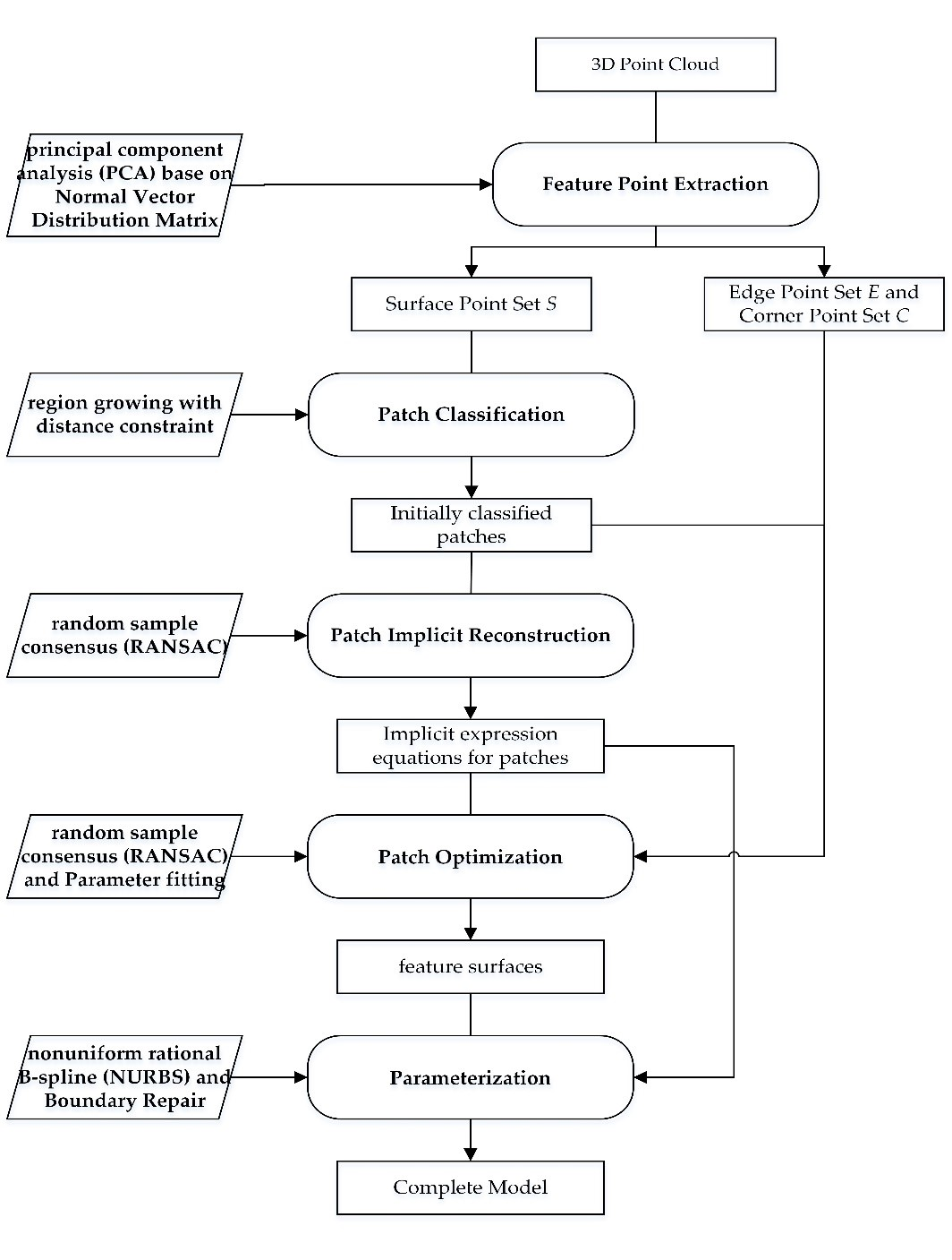
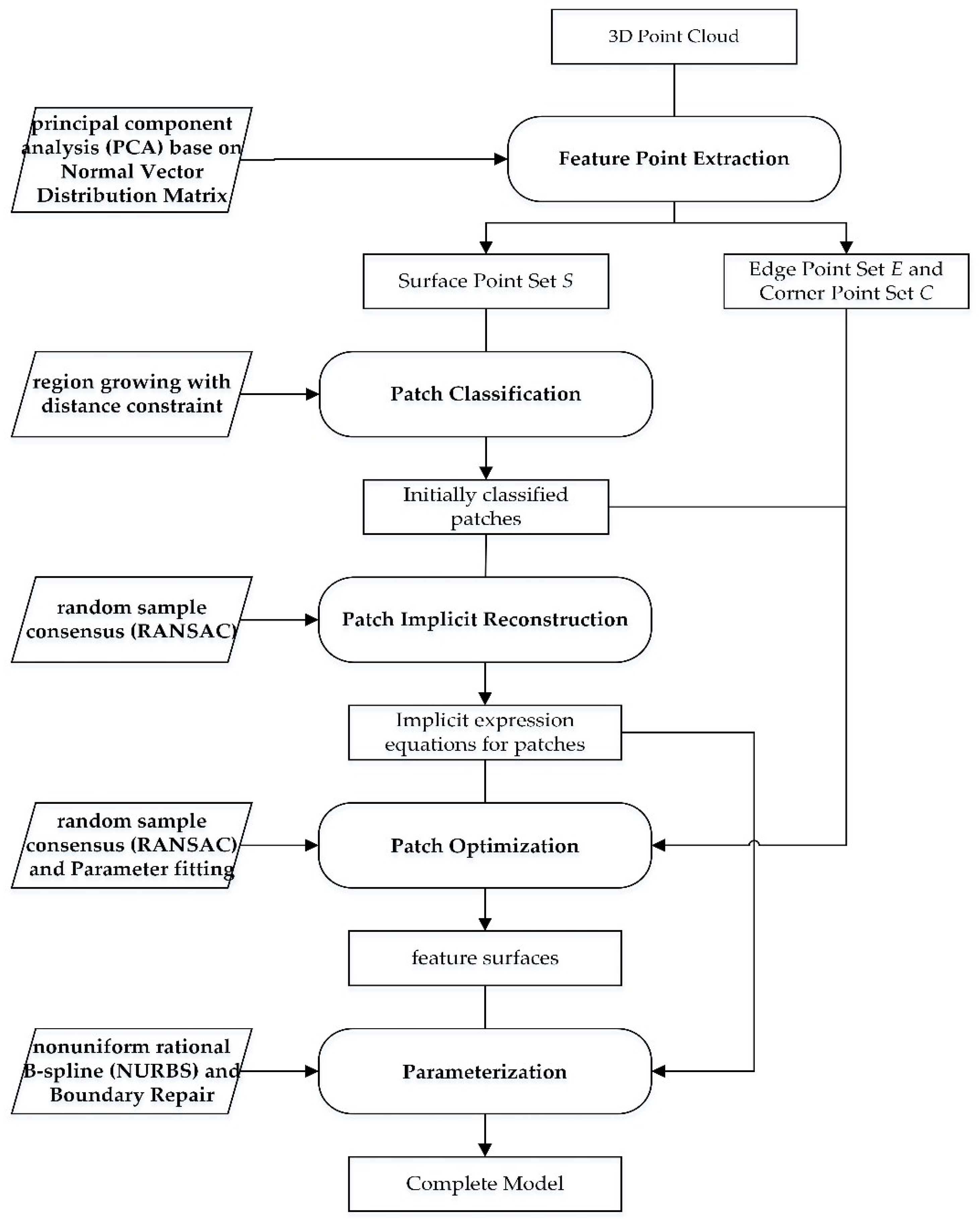
2. Method
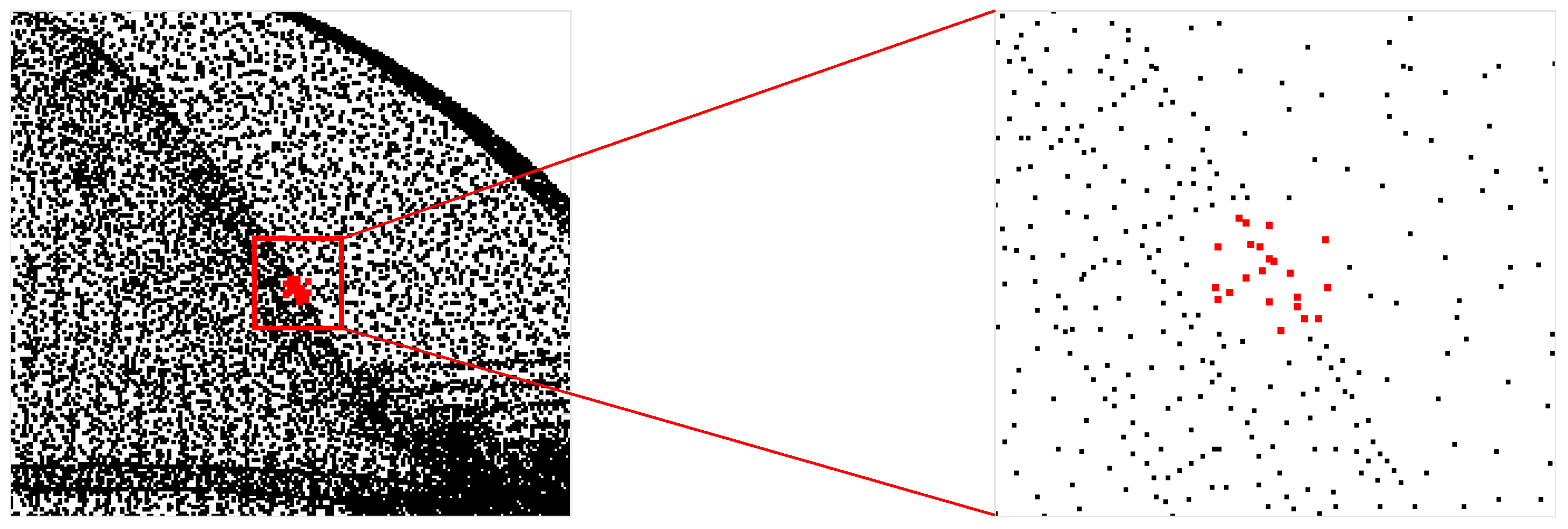
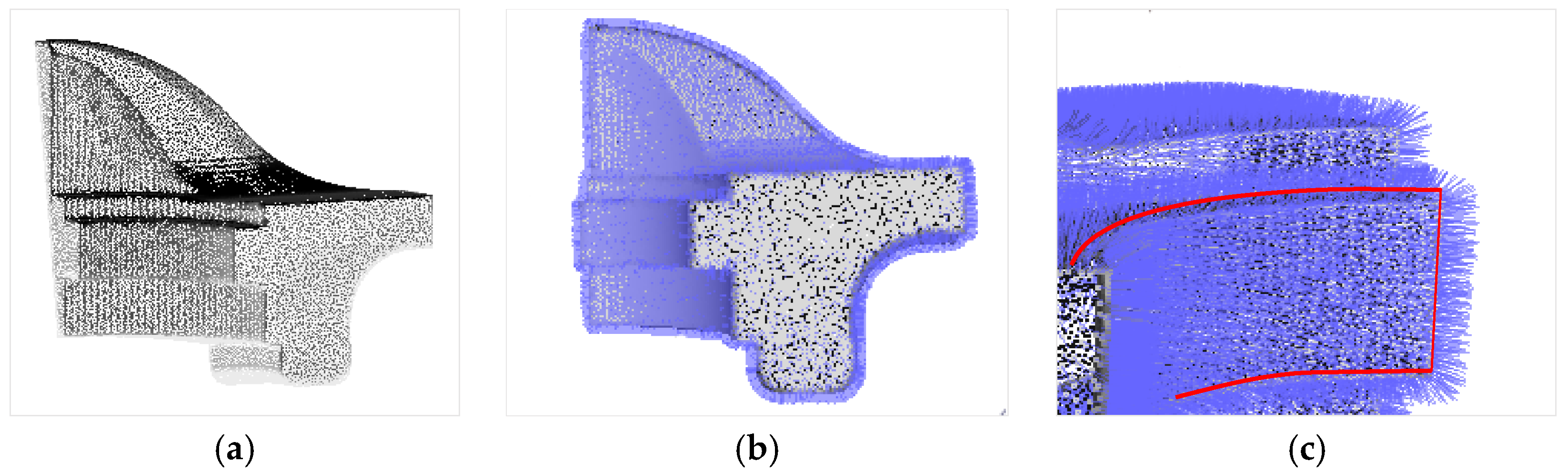
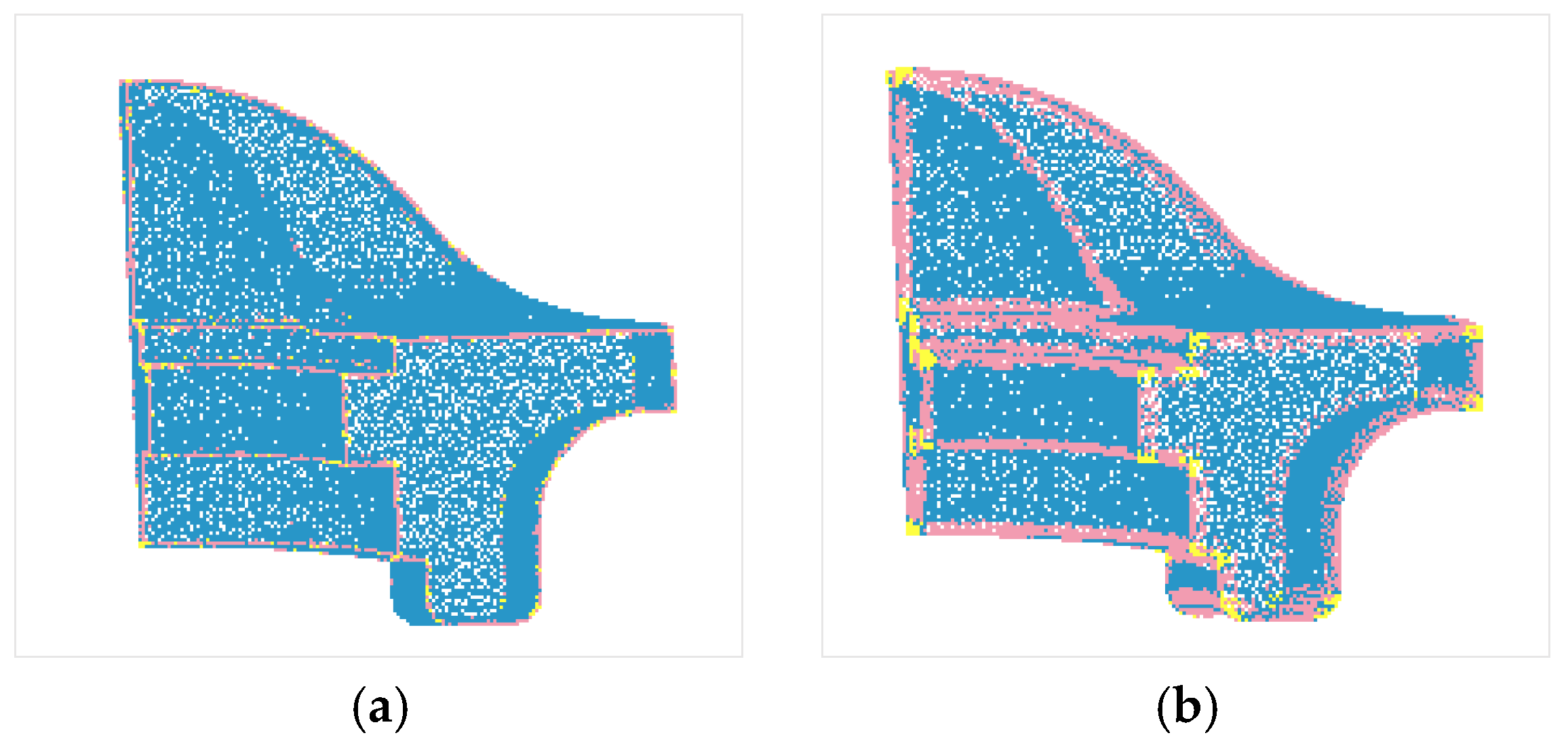
2.1. Feature Point Segmentation Based on the Normal Vector Distribution Matrix
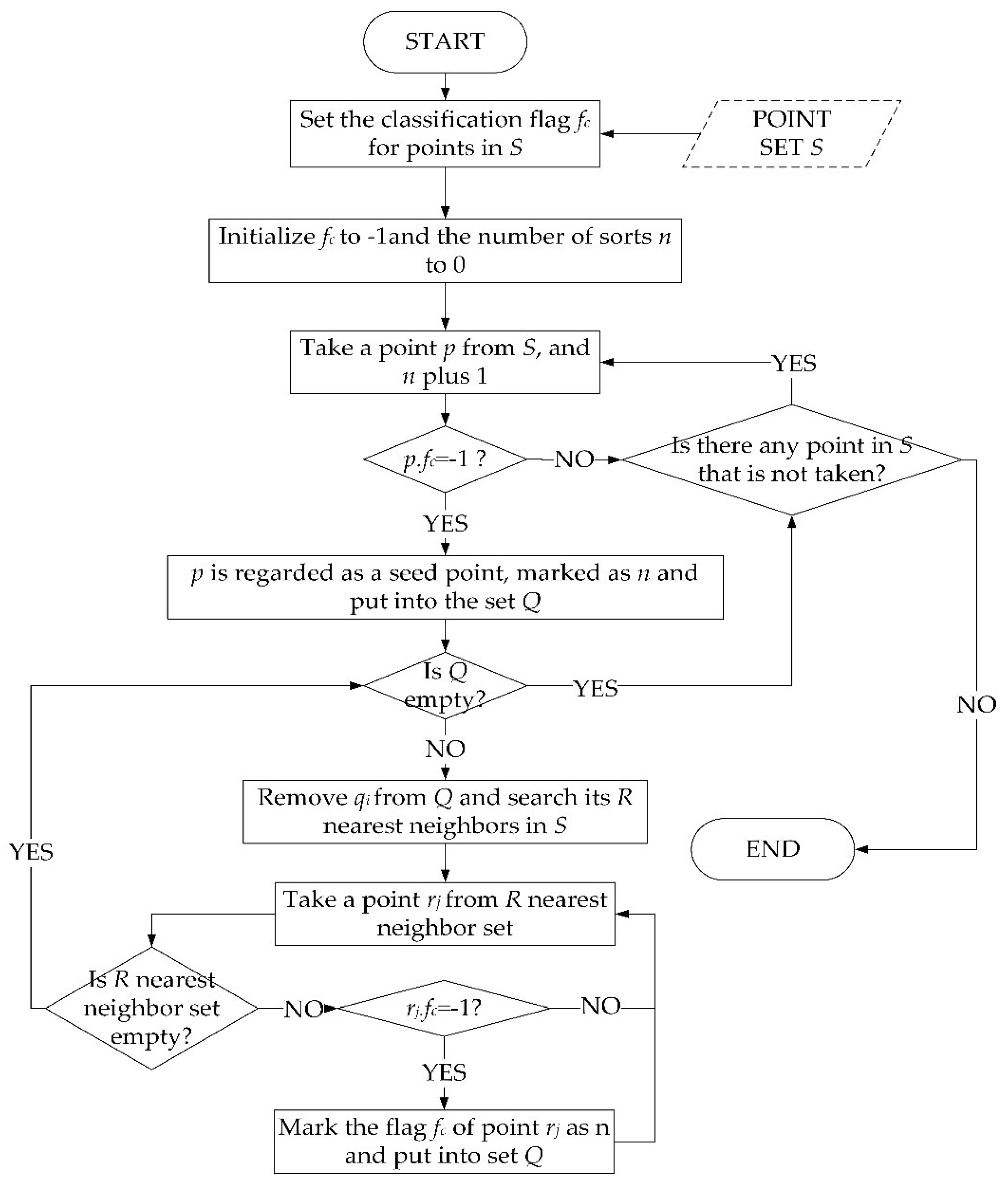
2.2. Patch Classification
- A classification flag fc is set for each point in surface point set S. The flag is initialized to −1, and the number of sorts, n, is initialized to 0.
- The algorithm is terminated when all the points in point set S are extracted. Otherwise, n is incremented, and a point p is extracted from point set S to determine whether its classification flag fc is −1 one by one. fc is regarded as a seed point, marked as n, and stored in the temporary point set Q when its value is −1. If fc is not −1, another point is obtained from S.
- If set Q is empty, then Step 2 is repeated. Otherwise, element qi is removed from Q, and the R nearest neighbors set of qi is searched.
- Flag fc of point rj in the R nearest neighbors set of qi is marked as n and stored in set Q when its value is −1.
2.3. Surface Implicit Reconstruction
2.3.1. 3D Surface Model
2.3.2. Model Parameter Solution Based on the RANSAC Algorithm
- Three points are randomly extracted from Si when the number of iterations is less than n, and the cosine values c1, c2, and c3 of the angles between the normal vectors of the three points are calculated, and Step 2 is executed. When the number of cycles is equal to n, Step 4 is executed.
- The patch may be a plane if the angles among the three normal vectors are roughly equal, that is, the absolute values of c1, c2, and c3 are approximately 1. Four parameters of the plane are calculated, and the inliers of the parametric model are calculated. The frequency of the plane model is incremented by 1 when the number of inliers is greater than the threshold, and the optimal parameters are updated and Step 1 is executed. Otherwise, Step 3 is executed.
- The parameters of the cylindrical or sphere model are calculated using two points, and the third point is used for verification. The inliers of the parametric model are calculated when the third point satisfies the calculated model. The frequency of the cylindrical or sphere model is incremented by 1 when the number of inner points is greater than the threshold, and the optimal parameters are updated. Continue to Step 1.
- Point set Si does not conform to the above three models when the maximum frequency of the model is less than 3 after n iterations, and the model output is 0. Otherwise, the maximum probability model is calculated, all the model inliers under the corresponding optimal model parameters are optimized using the least squares method, and the obtained model parameters are the final outputs.
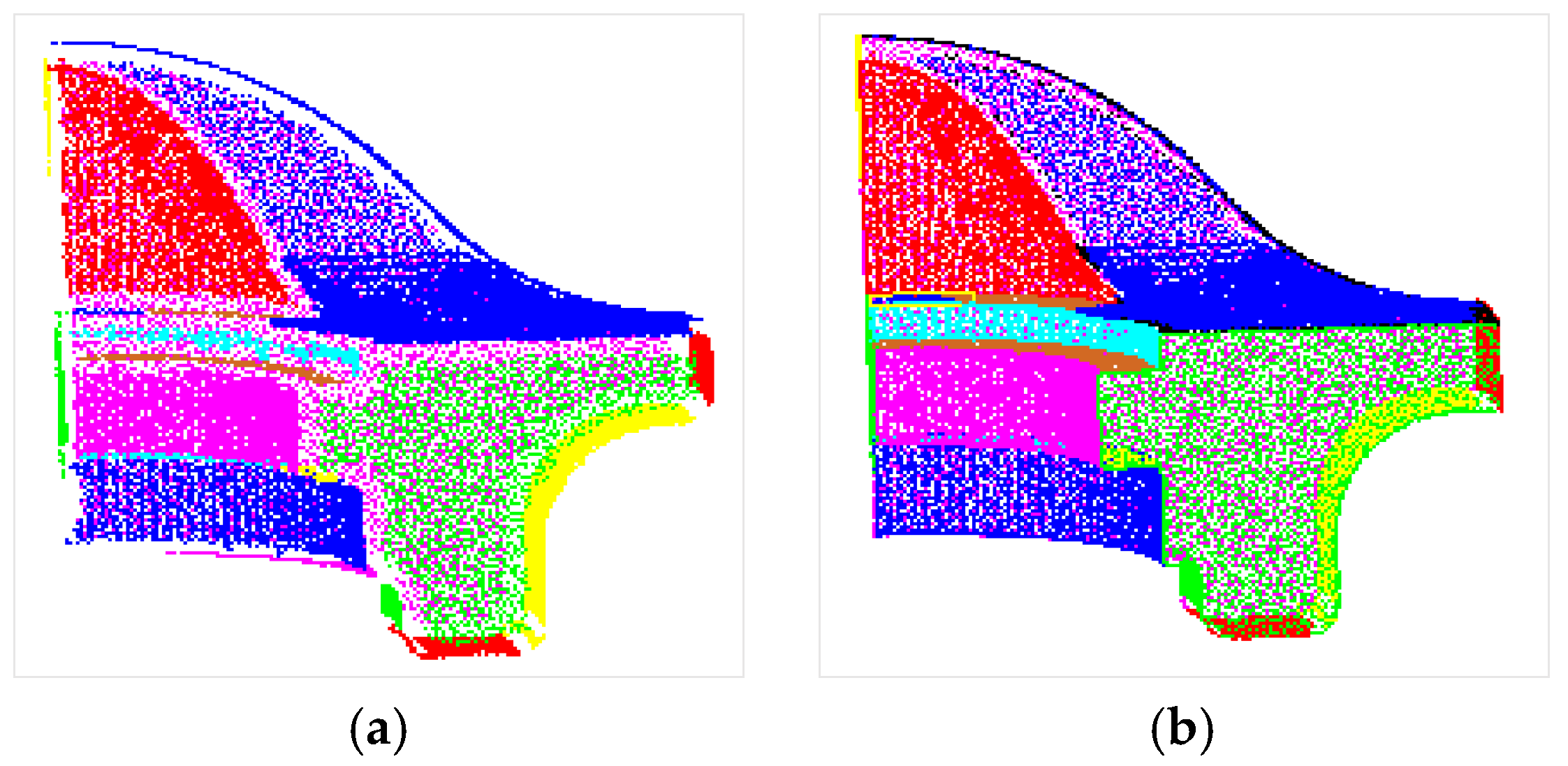
2.4. Patch Optimization
2.4.1. Patch Expansion
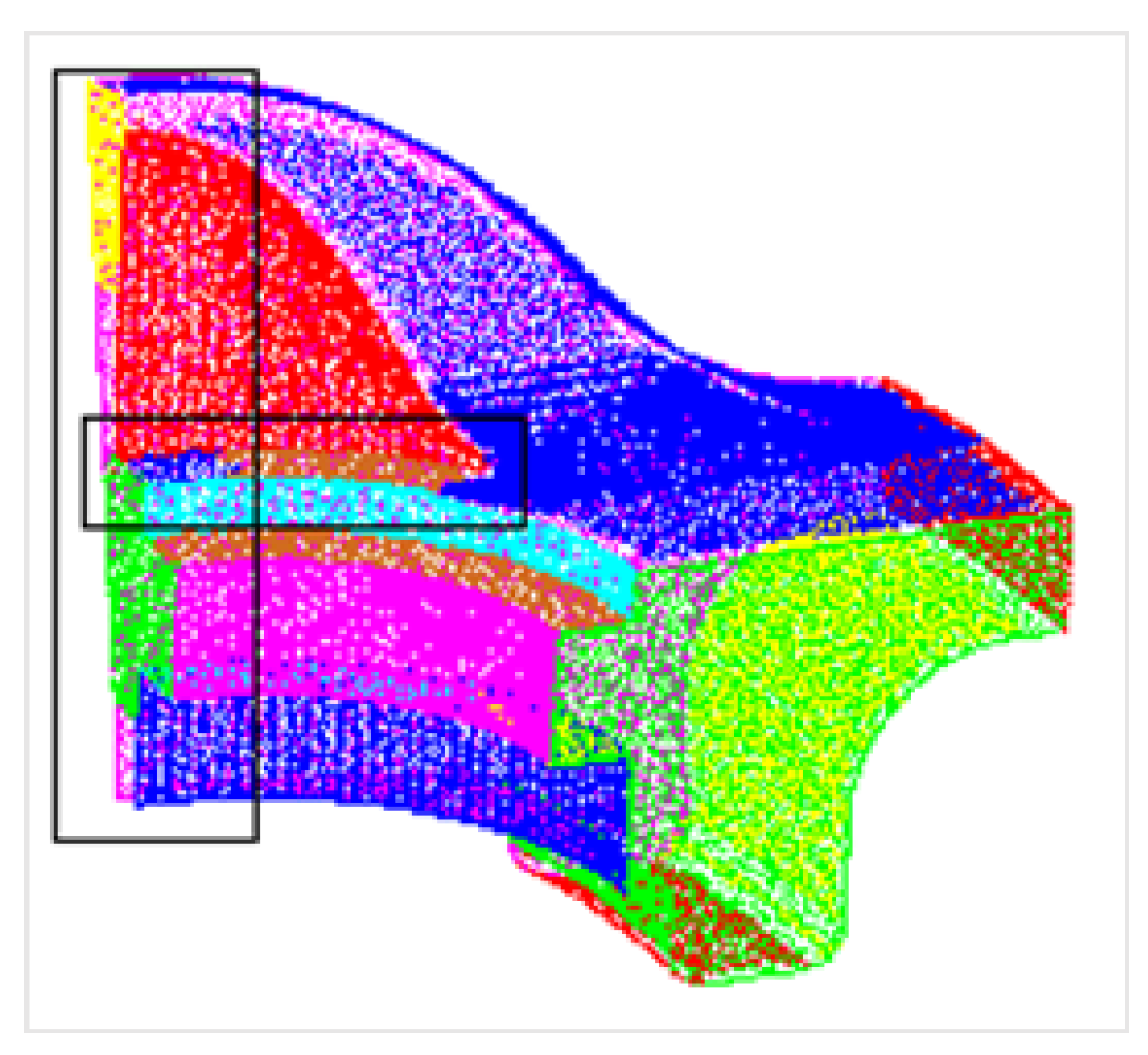
2.4.2. Patch Merging and Resegmentation
2.5. Surface Parameterization
3. Experiment and Results
3.1. Testing Data
3.2. Parameter Tuning
3.3. Results
4. Discussion
4.1. Comparative Studies
4.2. Result Analysis
4.3. Error Analysis
5. Conclusions
Author Contributions
Funding
Acknowledgments
Conflicts of Interest
References
- Lin, Y.; Wang, C.; Cheng, J. Line segment extraction for large scale unorganized point clouds. ISPRS J. Photogramm. Remote Sens. 2015, 102, 172–183. [Google Scholar] [CrossRef]
- Li, L.; Li, C.; Tang, Y.; Du, Y. An Integrated Approach of Reverse Engineering Aided Remanufacturing Process for Worn Components. Robot. Comput. Robot. Integr. Manuf. 2017, 48, 39–50. [Google Scholar] [CrossRef]
- Patel, M.; Desai, H. A Qualitative Survey on 3D Data Acquisition Techniques. Int. J. Sci. Res. Dev. 2015, 3, 781–785. [Google Scholar]
- Zheng, S.; Wang, X.; Ma, D. A Convenient 3D Reconstruction Method of Small Objects. Geomat. Inf. Sci. Wuhan Univ. 2015, 40, 147–152. [Google Scholar]
- Ni, H.; Lin, X.; Ning, X.; Zhang, J. Edge Detection and Feature Line Tracing in 3D-Point Clouds by Analyzing Geometric Properties of Neighborhoods. Remote Sens. 2016, 8, 710. [Google Scholar] [CrossRef]
- Zhang, Y. Research on Automatic Pipe Network Modeling Based on 3D Point Cloud Data. Master’s Thesis, Beijing University of Civil Engineering and Architecture, Beijing, China, 2016. [Google Scholar]
- Várady, T.; Facello, M.; Terék, Z. Automatic extraction of surface structures in digital shape reconstruction. Comput. Aided Des. 2007, 39, 379–388. [Google Scholar] [CrossRef]
- Li, J.; Wang, R. Robust Denoising of Point-sampled Surfaces. WSEAS Trans. Comput. 2009, 8, 153–162. [Google Scholar]
- Cao, J.; Li, X.; Chen, Z.; Qin, H. Spherical DCB-Spline Surfaces with Hierarchical and Adaptive Knot Insertion. IEEE Trans. Vis. Comput. Graph. 2012, 18, 1290–1303. [Google Scholar] [PubMed]
- Hu, J.; Wang, X.; Qin, H. Improved, Feature-centric EMD for 3D surface modeling and processing. Graph. Models 2014, 76, 340–354. [Google Scholar] [CrossRef]
- Merigot, Q.; Ovsjanikov, M.; Guibas, L. Voronoi-Based Curvature and Feature Estimation from Point Clouds. IEEE Trans. Comput. 2010, 17, 743–756. [Google Scholar] [CrossRef] [PubMed]
- Altantsetseg, E.; Muraki, Y.; Matsuyama, K.; Konno, K. Feature line extraction from unorganized noisy point clouds using truncated Fourier series. Vis. Comput. 2013, 29, 617–626. [Google Scholar] [CrossRef]
- Demarsin, K.; Vanderstraeten, D.; Roose, D. Meshless Extraction of Closed Feature Lines Using Histogram Thresholding. Comput.-Aided Des. Appl. 2013, 5, 589–600. [Google Scholar] [CrossRef]
- An, Y. Geometric Properties Estimation and Feature Identification from 3D Point Cloud. Ph.D. Thesis, Dalian University of Technology, Dalian, China, 2011. [Google Scholar]
- Zou, D. The Feature Extraction and Segmentation Analysis of Point Clouds. Ph.D. Thesis, Nanjing Normal University, Nanjing, China, 2012. [Google Scholar]
- Zhang, Y.; Geng, G.; Wei, X.; Su, H.; Zhou, M. Point Clouds Simplification with Geometric Feature Reservation. J. Comput.-Aided Des. Comput. Graph. 2016, 28, 1420–1427. [Google Scholar]
- Angelo, L.; Stefano, P. Geometric segmentation of 3D scanned surfaces. Comput. Aided Des. 2015, 62, 44–56. [Google Scholar] [CrossRef]
- Liu, Z.; Jiang, K.; Lin, J. Interactive extraction of boundary of specified target feature on scattered point cloud. Comput. Eng. Appl. 2016, 52, 186–190. [Google Scholar]
- Qin, J.; Wan, Y.; He, P.; Chen, M.; Lu, W.; Wang, S. An Automatic Building Boundary Extraction Method of TLS Data. Remote Sens. Inf. 2015, 30, 3–7. [Google Scholar]
- Berger, M.; Tagliasacchi, A.; Seversky, L.; Alliez, P.; Guennebaud, G.; Levine, J.; Sharf, A.; Silva, G. A Survey of Surface Reconstruction from Point Clouds. Comput. Graph. Forum 2016, 36, 301–329. [Google Scholar] [CrossRef]
- Kazhdan, M.; Bolitho, M.; Hoppe, H. Poisson Surface Reconstruction. In Proceedings of the EG/SIGGRAPH Symposium on Geometry Processing, Boston, MA, USA, 13–17 August 2006; pp. 61–70. [Google Scholar]
- Liu, S.; Wang, C. Orienting Unorganized Points for Surface Reconstruction. Comput. Graph. 2010, 34, 209–218. [Google Scholar] [CrossRef]
- Kai, W.; Bo, P. Feature curve extraction from point clouds via developable strip intersection. J. Comput. Des. Eng. 2015, 3, 102–111. [Google Scholar]
- Lu, X.; Yao, J.; Tu, J.; Li, K.; Li, L.; Liu, Y. Pairwise Linkage for Point Cloud Segmentation. ISPRS Ann. Photogramm. Remote Sens. Spat. Inf. Sci. 2016, 3, 201–208. [Google Scholar] [CrossRef]
- Mizoguchi, T.; Date, H.; Kanai, S.; Kishinami, T. Segmentation of scanned mesh into analytic surfaces based on robust curvature estimation and region growing. In Proceedings of the 4th International Conference on Geometric Modeling and Processing, Pittsburgh, PA, USA, 26–28 July 2006; pp. 644–654. [Google Scholar]
- Vo, A.; Truong-Hong, L.; Laefer, D.; Bertolotto, M. Octree-based region growing for point cloud segmentation. ISPRS J. Photogramm. Remote Sens. 2015, 104, 88–100. [Google Scholar] [CrossRef]
- Wang, X.; Zou, L.; Shen, X.; Ren, Y.; Qin, Y. A Region-growing Approach for Automatic Outcrop Fracture Extraction from A Three-dimensional Point Cloud. Comput. Geosci. 2017, 99, 100–106. [Google Scholar] [CrossRef]
- Schnabel, R.; Wahl, R.; Klein, R. Efficient RANSAC for Point-cloud Shape Detection. Comput. Graph. Forum 2007, 26, 214–226. [Google Scholar] [CrossRef]
- Arikan, M.; Wimmer, M.; Maierhofer, S. O-snap: Optimization-based Snapping for Modeling Architecture. ACM Trans. Graph. 2013, 32, 1–15. [Google Scholar] [CrossRef]
- Zeineldin, R.; El-Fishawy, N. A Survey of RANSAC Enhancements for Plane Detection in 3D Point Clouds. Menoufia J. Electron. Eng. 2017, 26, 519–537. [Google Scholar]
- Wu, S. Feature Extraction and Shape Detection in Reverse Engineering. Master’s Thesis, Zhejiang University, Hangzhou, China, 2011. [Google Scholar]
- Fuhrmann, S.; Goesele, M. Fusion of Depth Maps with Multiple Scales. In Proceedings of the ACM SIGGRAPH Asia Conference, HongKong, China, 12–15 December 2011. [Google Scholar]
- Tagliasacchi, A.; Olson, M.; Zhang, H.; Hamarneh, G.; Cohen-Or, D. VASE: Volume-Aware Surface Evolution for Surface Reconstruction from Incomplete Point Clouds. Comput. Graph. Forum 2011, 30, 1563–1571. [Google Scholar] [CrossRef] [Green Version]
- Wu, G.; Zhang, Y. A Novel Fractional Implicit Polynomial Approach for Stable Representation of Complex Shapes. J. Math. Imaging Vis. 2017, 55, 89–104. [Google Scholar] [CrossRef]
- Rouhani, M.; Sappa, A.; Boyer, E. Implicit B-spline Surface Reconstruction. IEEE Trans. Image Process. 2015, 24, 22–32. [Google Scholar] [CrossRef] [PubMed]
- Xu, L.; Wu, G. Review of Implicit Surface Reconstruction from Point Cloud Dataset. Comput. Sci. 2017, 44, 19–23. [Google Scholar]
- Bohm, W.; Farin, G.; Kahmann, J. A Survey of curve and surface methods in CAGD. Comput. Aided Geom. Des. 1984, 1, 1–60. [Google Scholar] [CrossRef]
- Barazzetti, L.; Banfi, F.; Brumana, R.; Previtali, M. Creation of Parametric BIM Objects from Point Clouds Using Nurbs. Photogramm. Rec. 2016, 30, 339–362. [Google Scholar] [CrossRef]
- Fu, H.; Liu, X.; Li, J. NURBS Surface Reconstruction Based on Terrestrial LiDAR Point Cloud. J. Geomat. 2017, 42, 17–19. [Google Scholar]
- Linsen, L.; Prautzsch, H. Local versus global triangulations. In Proceedings of the Eurographics, Manchester, UK, 5–7 September 2001; pp. 257–263. [Google Scholar]
- Pauly, M.; Keiser, R.; Kobbelt, L.; Gross, M. Shape modeling with point-sampled geometry. ACM Trans. Graph. 2003, 22, 641–650. [Google Scholar] [CrossRef]
- Hoppe, H.; Derose, T.; Duchamp, T.; Mcdonald, J.; Stuetzle, W. Surface Reconstruction from Unorganized Points. In Proceedings of the 19th Annual Conference on Computer Graphics and Interactive Techniques, New York, NY, USA, 26–31 July 1992; pp. 71–78. [Google Scholar]
- PCL-The Point Cloud Library. 2012. Available online: http:// pointclouds.org/ (accessed on 12 April 2018).
- Roth, G.; Levine, M. Geometric Primitive Extraction Using a Genetic Algorithm. IEEE Trans. Pattern Anal. Mach. Intell. 1994, 16, 901–905. [Google Scholar] [CrossRef]
- Li, Z.; Li, D.; Li, Z.; Wang, Z. New method on extracting geometric primitives. Infrared Laser Eng. 2001, 30, 4–7. [Google Scholar]
- Weber, C.; Hahmann, S.; Hagen, H.; Bonneau, G. Sharp Feature Preserving MLS Surface Reconstruction based on Local Feature Line Approximations. Graph. Models 2012, 74, 335–345. [Google Scholar] [CrossRef]
- Zeng, C.; Wang, J.; Lehrbass, B. An Evaluation System for Building Footprint Extraction from Remotely Sensed Data. IEEE J. Sel. Top. Appl. Earth Obs. Remote Sens. 2013, 6, 1640–1652. [Google Scholar] [CrossRef]
- Truong-Hong, L.; Laefer, D. Quantitative evaluation strategies for urban 3D model generation from remote sensing data. Comput. Graph. 2015, 49, 82–91. [Google Scholar] [CrossRef] [Green Version]
- Fu, W.; Zhang, H. Reverse Engineering Design Based on Geomagic Studio Software. Tool Eng. 2007, 41, 54–57. [Google Scholar]
- Zhou, X. Piecewise Method for Large Scale Reconstruction and Optimization. Master’s Thesis, Zhejiang University, Hangzhou, China, 2017. [Google Scholar]
- Cheng, S.; Wang, Y. Reconstructing Piecewise Curved Complexes. Surf. Reconstr. 2008. Available online: http://hdl.handle.net/1783.1/3090 (accessed on 8 May 2018).


| Steps | Notation | Explanations | |
|---|---|---|---|
| Segmentation Based on Point Coordinates | Segmentation Based on Normal Vector | ||
| Search for K nearest neighbor points | p | p | Discrete point |
| K | K | Number of nearest neighbor points | |
| Q | Q | K nearest neighbor set | |
| qi | qi | ith point of K nearest neighbor set | |
| Fit local plane | - | P | Fitting local plane |
| - | d | Distance between point p and fitting plane P | |
| - | n | Normal vector of the fitting plane | |
| - | ith projection point of a neighbor point on the fitting plane | ||
| - | θ | Weight function | |
| Calculate normal vector of discrete points | - | C | Covariance matrix constructed by point’s coordinate |
| - | Center of gravity of point set Q | ||
| - | ni | ith normal vector of discrete points | |
| PCA | C | A | Covariance matrix constructed by point’s coordinate or normal vector |
| - | Center of gravity of the point set Q | ||
| λci (i = 1, 2, 3) | λi (i = 1, 2, 3) | ith eigenvalues | |
| Segment feature points | δci (i = 1, 2, 3) | δi (i = 1, 2, 3) | ith normalized eigenvalues |
| ec0 | e0 | First threshold | |
| ec1 | e1 | Second threshold | |
| Model | Surfaces | Points | Average Point Spacing (dm) | Minimum Point Spacing (dm) | Bounding Box Size | ||
|---|---|---|---|---|---|---|---|
| Boxx (dm) | Boxy (dm) | Boxz (dm) | |||||
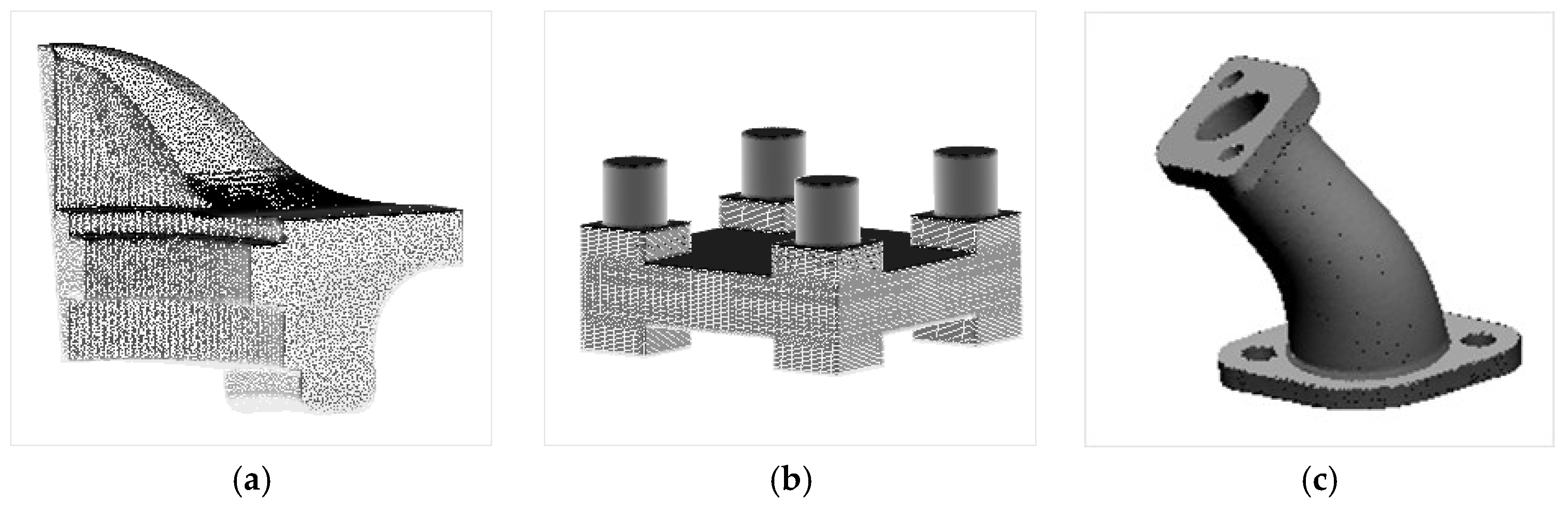
| Fandisk model | 21 | 55,105 | 0.0426 | 0.006 | 4.8281 | 5.2445 | 2.6805 |
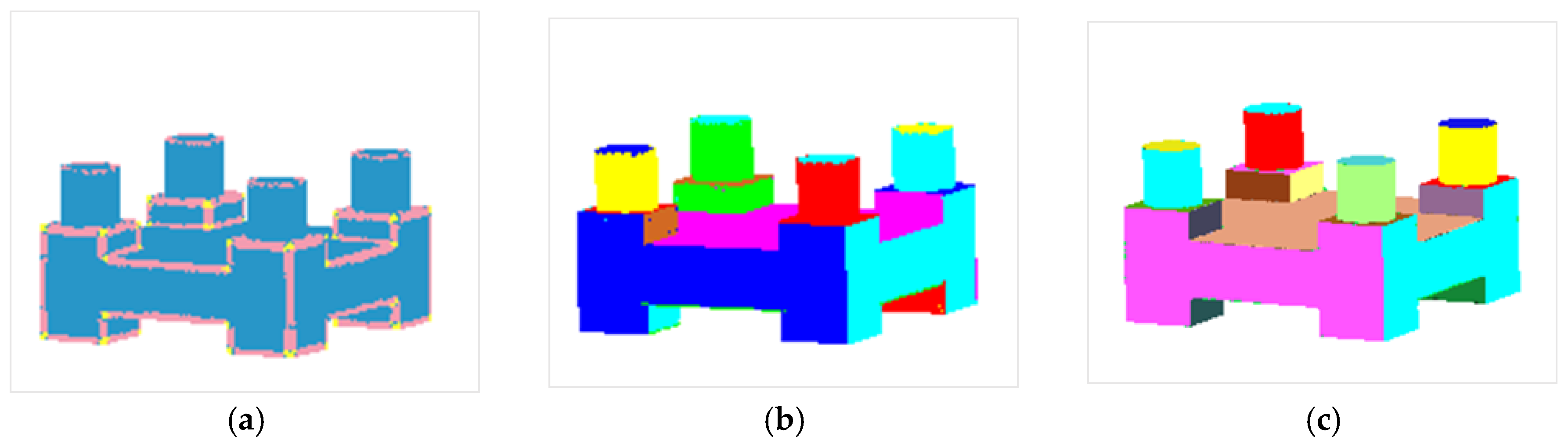
| Support frame model | 38 | 200,018 | 0.0052 | 0.0002 | 1.0000 | 1.0000 | 0.6000 |
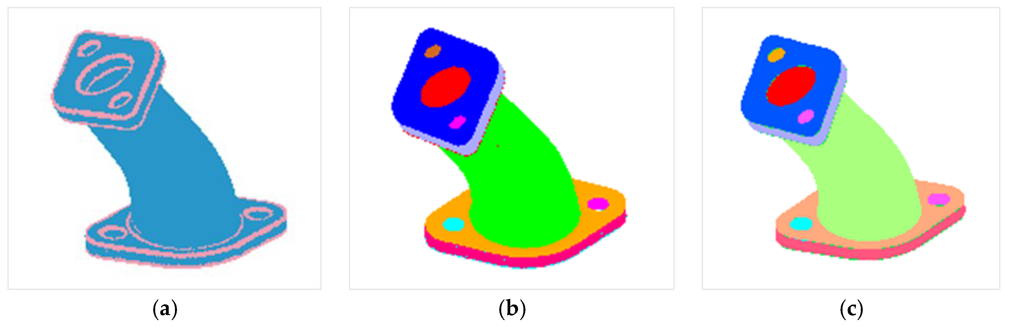
| Connecting piece model | 12 | 1,514,884 | 0.0024 | 0.0005 | 0.9975 | 0.9264 | 0.7838 |
| Parameter | Fandisk Model | Support Frame Model | Connecting Piece Model |
|---|---|---|---|
| K (ea) | 15 | 16 | 20 |
| e0 | 0.0045 | 0.005 | 0.035 |
| e1 | 0.006 | 0.01 | 0.1 |
| n1 (time) | 125 | 25 | 55 |
| n2 (time) | 200 | - | 150 |
| κ (ea) | 600 | - | 1000 |
| μ (dm) | 0.35 | - | 0.025 |
| R (dm) | 0.07 | 0.02 | 0.02 |
| ε (dm) | 0.006 | 0.005 | 0.002 |
| Model | Nap | Ntp | Nmp | Nop |
|---|---|---|---|---|
| Fandisk model | 55,105 | 54,688 | 222 | 195 |
| Support frame model | 200,018 | 199,693 | 218 | 107 |
| Connecting piece model | 151,484 | 149,943 | 220 | 1321 |
| Model | Corr (%) | Comp (%) | Qual (%) | T (s) |
|---|---|---|---|---|
| Fandisk model | 99.60 | 99.64 | 99.24 | 54.36 |
| Support frame model | 99.89 | 99.95 | 99.84 | 22.55 |
| Connecting piece model | 99.85 | 99.13 | 98.98 | 43.29 |
| Method | Points | Execution Time (s) | Qual (%) |
|---|---|---|---|
| Zhou [50] | 23,400 | 79 | 99.04 |
| Cheng et al. [51] | 66,100 | 140.88 | - |
| Our method | 55,105 | 54.36 | 99.24 |
| Method | Points | Control Points | Qual (%) |
|---|---|---|---|
| Cao et al. [9] | 56,000 | 582 | 98.84 |
| 4994 | 99.97 | ||
| Our method | 55,105 | 0 | 99.24 |
© 2018 by the authors. Licensee MDPI, Basel, Switzerland. This article is an open access article distributed under the terms and conditions of the Creative Commons Attribution (CC BY) license (http://creativecommons.org/licenses/by/4.0/).
Share and Cite
Wang, Y.; Wang, J.; Chen, X.; Chu, T.; Liu, M.; Yang, T. Feature Surface Extraction and Reconstruction from Industrial Components Using Multistep Segmentation and Optimization. Remote Sens. 2018, 10, 1073. https://0-doi-org.brum.beds.ac.uk/10.3390/rs10071073
Wang Y, Wang J, Chen X, Chu T, Liu M, Yang T. Feature Surface Extraction and Reconstruction from Industrial Components Using Multistep Segmentation and Optimization. Remote Sensing. 2018; 10(7):1073. https://0-doi-org.brum.beds.ac.uk/10.3390/rs10071073
Chicago/Turabian StyleWang, Yuan, Jiajing Wang, Xiuwan Chen, Tianxing Chu, Maolin Liu, and Ting Yang. 2018. "Feature Surface Extraction and Reconstruction from Industrial Components Using Multistep Segmentation and Optimization" Remote Sensing 10, no. 7: 1073. https://0-doi-org.brum.beds.ac.uk/10.3390/rs10071073